the Creative Commons Attribution 4.0 License.
the Creative Commons Attribution 4.0 License.
 | 09 Jun 2021
Space variability impacts on hydrological responses of nature-based solutions and the resulting uncertainty: a case study of Guyancourt (France)
Igor da Silva Rocha Paz
Feihu Chen
Pierre-Antoine Versini
Daniel Schertzer
Ioulia Tchiguirinskaia
During the last few decades, the urban hydrological cycle has been strongly modified by the built environment, resulting in fast runoff and increasing the risk of waterlogging. Nature-based solutions (NBSs), which apply green infrastructures, have been more and more widely considered as a sustainable approach for urban storm water management. However, the assessment of NBS performance still requires further modelling development because of hydrological modelling results strongly depend on the representation of the multiscale space variability of both the rainfall and the NBS distributions. Indeed, we initially argue this issue with the help of the multifractal intersection theorem. To illustrate the importance of this question, the spatial heterogeneous distributions of two series of NBS scenarios (porous pavement, rain garden, green roof, and combined) are quantified with the help of their fractal dimension. We point out the consequences of their estimates. Then, a fully distributed and physically based hydrological model (Multi-Hydro) was applied to consider the studied catchment and these NBS scenarios with a spatial resolution of 10 m. A total of two approaches for processing the rainfall data were considered for three rainfall events, namely gridded and catchment averaged. These simulations show that the impact of the spatial variability in rainfall on the uncertainty of peak flow of NBS scenarios ranges from about 8 % to 18 %, which is more significant than those of the total runoff volume. In addition, the spatial variability in the rainfall intensity at the largest rainfall peak responds almost linearly to the uncertainty of the peak flow of NBS scenarios. However, the hydrological responses of NBS scenarios are less affected by the spatial distribution of NBSs. Finally, the intersection of the spatial variability in rainfall and the spatial arrangement of NBSs produces a somewhat significant effect on the peak flow of green roof scenarios and the total runoff volume of combined scenarios.
- Article
(9626 KB) - Full-text XML
- BibTeX
- EndNote


The increased risk of flooding from urban storms appears to be closely linked to the following two key factors: rapid urbanization and climate change (Lovejoy and Schertzer, 2013). Adapting to climate change and mitigating urban flooding now constitute significant societal challenges (Loukas et al., 2010; Miller and Hutchins, 2017). Impervious surfaces directly connected to grey infrastructures result in a rapid transfer of rainfall into runoff, which greatly increases the risk of flooding, especially in urban watersheds (Fry and Maxwell, 2017; Ercolani et al., 2018). Expanding and upgrading the capacity of existing drainage systems has proven to be costly and unsustainable, which is challenging to realize in highly urbanized cites (Qin et al., 2013).
Increasing urban resilience to reduce the risk of urban flooding has been emphasized in many countries (e.g. Kelman, 2015). Nature-based solutions (NBSs) refer to a sustainable strategy, capable of reducing the influences of human activities on the natural environment, which is especially efficient for storm water management (European Commission, 2015; Cohen-Shacham et al., 2016). To some extent, the NBS concept builds on and supports similar, widely used concepts (Bozovic et al., 2017), like the low-impact development (LID), or Blue–Green Infrastructure (BGI), and some more local ones, like the water-sensitive urban design (WSUD), from Australia (Morison and Brown, 2011), or a “sponge city”, proposed recently in China (Chan et al., 2018). Regarding storm water management, NBSs suggests using a suite of small-scale controlled measures. This often includes bio-retention swale, porous pavement, green roof, rain garden, and rain barrel because these infrastructures are able to conserve or recover the natural environment of a region (Newcomer et al., 2014).
The hydrological performances of such NBSs have been approached in terms of the reduction of total runoff volume and peak flow at the urban catchment scale (Zahmatkesh et al., 2015; Ahiablame and Shakya, 2016; Bloorchian et al., 2016). Generally, the results of a large number of studies are based on lumped or semi-distributed models (Ahiablame et al., 2013; Liu et al., 2015; Massoudieh et al., 2017; Guo et al., 2019). Indeed, as underlined by Fry and Maxwell (2017) and Her et al. (2017), fully distributed models are rarely used (Versini et al., 2016; Hu et al., 2017; Versini et al., 2018). While there is a general consensus that these models should better assess the hydrological performances of NBSs implemented at smaller scales, the deployment of the fully distributed models has been stuck for some time by the following three main factors: (i) availability of reliable, high-resolution forcing, (ii) complex interactions between the processes, and (iii) a reliable parameterization process (e.g. Imhoff et al., 2020). As a consequence, the semi-distributed Storm Water Management Model (SWMM) remains the one that is most frequently used to investigate the impact of NBSs on urban runoff and water quality (Sun et al., 2014; Jia et al., 2015; Palla et al., 2015; Cipolla et al., 2016; Kwak et al., 2016). Nevertheless, Rossman et al. (2010) demonstrated that SWMM has some serious limitations for reflecting the heterogeneity of urban watersheds, which in turn presents some difficulties for sustainably replicating hydrological responses to various urban land uses. In particular, the study of Burszta-Adamiak and Mrowiec (2013) confirmed that SWMM is not really explicit for presenting the hydrological responses of catchments with only the help of the percentage of pervious and impervious land covers. These gaps imply strong limitations to the results obtained with the help of lumped and the semi-distributed models. Thus, to make the modelling results more accurate and credible, there is a strong need to use fully distributed and physically based models.
At the same time, due to the long-standing challenge of the availability of reliable and high-resolution spatio-temporal precipitation measurements in urban areas, some studies have been devoted to assessing the performance of NBSs under the simplifying assumption of a uniform rainfall; hence, the impact of spatial rainfall variability in the heterogeneous urban context has not been considered (Holman-Dodds et al., 2003; Gilroy and McCuen, 2009; Qin et al., 2013; Versini et al., 2018; Zhu et al., 2019; Guo et al., 2019). A strong impact of the temporal variability in precipitation on the response of the watershed is generally well recognized (Schertzer et al., 2010; Ochoa-Rodriguez et al., 2015; Gires et al., 2015). Qin et al. (2013) also investigated the performance of some NBSs, such as swales, porous pavements, and green roofs, as a function of peak precipitation intensity. Whereas the temporal variability in precipitation, even intuitively, forces the dynamics of the retention capacity of the NBSs, the impact of the spatial variability in precipitation in the heterogeneous urban context has not yet been studied in its full extent. However, the hydrological responses of NBSs (model outputs) can largely depend on the following: (i) the highly spatially variable rainfall fields, (ii) the spatial distribution of the NBSs, and (iii) their intersection. Indeed, the rainfall and the NBSs represent two heterogeneous fields that do not coincide, which implies that the overall performances of NBS scenarios simulated with uniform rainfall or lumped and/or semi-distributed model may not be entirely convincing. Therefore, the mentioned impacts remain to be investigated, especially for higher spatial model resolutions, using spatio-temporal rainfall fields with a fully distributed model, allowing heterogeneous NBS scenarios.
In this respect, the main goal of this study is to investigate the uncertainty of hydrological responses in various NBS scenarios resulting from the spatial variability in rainfall and the heterogeneous distribution of NBSs at the urban catchment scale, and thus not those associated to the model structure, hypothesis, or parameterization, for instance. A fully distributed and physically based hydrological model, Multi-Hydro (Giangola-Murzyn, 2013; Ichiba et al., 2018), is applied on a semi-urban catchment of 5.2 km2 in the city of Guyancourt (France) at the scale of 10 m. The particularity of Multi-Hydro is its scalability, which makes it possible to replace the traditional parameter calibration by the process of rapid optimization of the spatio-temporal resolution of the model to ensure its best performance for the case study, based on the overall scaling of available data (Ichiba et al., 2018). Multi-Hydro is, therefore, well suited to achieving the desired objective of this study. A total of two different rainfall processing approaches (gridded and catchment-averaged) from three typical rainfall events of the Paris region are used as meteorological inputs, as follows: (i) based on the gridded approach, the data are retrieved from the X-band polarimetric radar of École des Ponts ParisTech (ENPC), characterized by high spatial and temporal resolutions, which are called distributed rainfall data, and (ii) the corresponding uniform rainfall data are obtained from the catchment average of the distributed rainfall data at each time step. The spatial heterogeneity of NBSs is grasped by different land use scenarios, characterized with the help of an across-scale indicator, namely the fractal dimension. This variability and the resulting uncertainties in hydrological responses of the catchment are quantified by considering the peak flow and the total runoff volume in the drainage conduits. It is important to mention here that a precise quantitative evaluation of NBS performances, e.g. peak discharge reduction, total runoff volume reduction, or both, is not the goal of the present study. The authors aim first to deepen the knowledge on the impact of the spatial variability in the rainfall on hydrological responses of several NBS scenarios, and that, in turn, helps to clarify whether the NBSs could be randomly implemented in semi-urban catchments or not.
The organization of this paper is as follows. The next section presents the study area, the rainfall data and the Multi-Hydro model. The details of the NBS scenarios, the framework of modelling experiments, and the model validation are described in Sect. 3. Then, the obtained results are discussed in Sect. 4. Finally, the main conclusions are summarized in Sect. 5.
2.1 The choice of the case study
This study is conducted on a semi-urban catchment, in a part of the city of Guyancourt (France), located on the Saclay Plateau in the southwestern suburb of Paris (Fig. 1). The available raw 25 m resolution digital elevation model (DEM) obtained from the French National Institute of Forest and Geographic Information (IGN), which presents the whole catchment, is relatively flat (see the left side of Fig. 1). The altitude in the north is slightly higher than that of the south. The highest altitude in the whole catchment reaches 175.1 m, while the lowest one of 143.39 m corresponds to the location of the storage basin (i.e. the outlet of the catchment – Etang des Roussières). The most recent statistical report of Météo-France (2020) indicates that the area is characterized by an oceanic climate with an average annual temperature of about 10.7 ∘C and total annual precipitation around 695 mm. In this context, the Guyancourt catchment is an interesting and appropriate case study for several reasons.
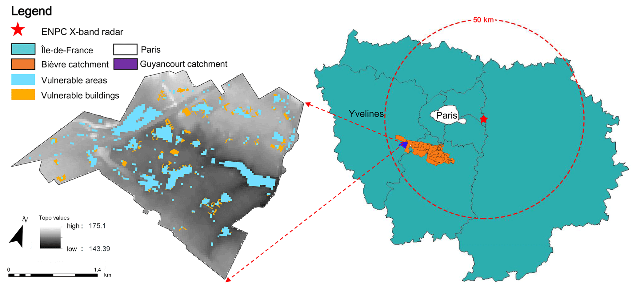
Figure 1Location of the study site and the corresponding topography map, highlighting some vulnerable areas and buildings at risk of waterlogging in the Guyancourt catchment.
First, Guyancourt is one of the subcatchments in the upstream of the 34.6 km long Bièvre river, which flows through several increasingly urbanized areas and joins the Seine river in Paris. The Bièvre river is well known by its drastic contribution to the historical 1910 flood in Paris and still easily generates flash floods during the heavy rainfall events (e.g. two severe floods occurred in 1973 and 1982). Therefore, the case of Guyancourt has a reference significance for the Paris region.
Second, the Guyancourt city is expected to become a part of the “French Silicon Valley”, which is currently undergoing a rapid urbanization process over its total area of around 5.2 km2, with a population of about 30 000 (INSEE, 2020). Based on the data from IGN, the current land use of the study area consists of seven main types, including road, parking, building, gully, forest, grass, and water. In total, these seven land use types cover 9.6 %, 10.6 %, 15.5 %, 1.9 %, 28.8 %, 32.7 %, and 0.9 % of the total area, respectively, as shown on the left side of Fig. 2. Currently, the pervious surface accounts for 62.4 % of the total area, and the corresponding impervious surface is 37.6 %.

Figure 2(a) Land use map (baseline scenario). (b) Drainage system with four conduits (4541, 4542, 4543, and 4544) highlighted.
The local authority, the agglomeration community of Saint-Quentin-en-Yvelines (la communauté d'agglomération de Saint-Quentin-en-Yveline), manages the urban drainage system of the catchment and provided some related data (right side of Fig. 2). The total length of the drainage system is about 76 km and consists of 4474 nodes and 4534 conduits. Overall, the drainage system was designed with a capacity characterized by a return period ranging from 2 to 10 years. The diameters of the conduits range between 0.1 and 1.6 m, with 70 % of them between 0.3 and 0.5 m (marked with a yellow line on the right side of Fig. 2). The conduits with a diameter ranging between 0.9 and 1.6 m (marked with a purple line on the right side of Fig. 2) are the primary conduits which converge the flow to the storage basin and the outlet. The rainfall amount corresponding to the mentioned return periods (from 2 to 10 years) depends on the considered duration (usually equal to the concentration time). So, this duration value depends on the location of pipes in the catchment and its upstream area. The following are the corresponding values for different durations that can be found on the studied watershed (by using the Montana coefficients): (i) duration 5 min – 187 mm h−1 for T= 10 years and 125 mm h−1 for T= 2 years; (ii) duration 30 min – 50 mm h−1 for T= 10 years and 31 mm h−1 for T= 2 years; (iii) duration 1 h – 30 mm h−1 for T= 10 years and 18 mm h−1 for T= 2 years; and (iv) duration 2 h – 20 mm h−1 for T= 10 years and 13 mm h−1 for T= 2 years.
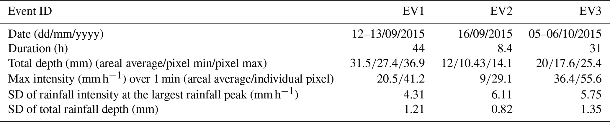
Regarding the properties of the three selected rainfall events (Table 1), the drainage system seems to have the capacity to drain the rainfall intensities on these durations. Nevertheless, we do not have any information about the exact duration range that was considered for the design (durations smaller than 30 min are usually not considered).
Table 1Main characteristics of selected rainfall events and standard deviation (SD) of the rainfall intensity at the largest rainfall peak and the total rainfall depth of the three rainfall events.
However, due to climate change, a clear tendency towards a growing number of shorter duration, but higher intensity, rainfall events is perceived for this region (Hoang, 2011), causing a large amount of fast surface runoff and higher peak flow rates in recent years. The existing storm water drainage system may not be able to sustain the future modifications of the watershed, and some low-lying areas in the catchment could suffer more easily from waterlogging, even during moderate rainfall. As Fig. 1 displays, some vulnerable areas and buildings subject to a risk of waterlogging were defined in the Guyancourt catchment by using the ModelBuilder of ArcGIS software (a geoprocessing model for identifying landscape sinks https://learn.arcgis.com/en/, last access: 2 June 2021). This geoprocessing model is based on a sequential chain of geographic information system (GIS) analysis tools. By exploring the digital elevation model (DEM) of the Guyancourt catchment with the ArcGIS desktop Hydrology tools (https://desktop.arcgis.com, last access: 2 June 2021), we first identify the landscape sinks. In this figure, the blue spots represent the low-lying areas with a total area of 0.6 km2 that can be easily flooded by storm water (average rainfall depth of 53 mm). Then, the locations of the landscape sinks can be compared with the locations of existing buildings, and the buildings that are situated inside or adjacent to the landscape sinks are defined as the vulnerable buildings. Correspondingly, the yellow spots indicate these vulnerable buildings in the figure.
Third, the local authority installed a gauge at the storage basin (outlet) to monitor water levels, which provided a measurement point of the Guyancourt catchment.
Overall, the relative complexity of the catchment makes it a typical case study for analysing some of the uncertainties related to hydrological responses of NBS scenarios, aiming to help the local authorities to find more reasonable and ecological alternatives for future urban planning.
2.2 Rainfall data
In this study, one of the purposes is to assess the impact of the spatial variability in rainfall on the hydrological responses of some NBS scenarios. Hence, the following two approaches for processing rainfall data were used to prepare the meteorological inputs: gridded (distributed) and catchment averaged (uniform). Based on the gridded approach, the distributed rainfall data were retrieved from the polarimetric X-band radar, located at ENPC, Champs-sur-Marne (east of Paris, France). The distance between the X-band radar and the catchment is around 45 km (see Fig. 1). The spatial and temporal resolutions of the X-band radar are 250 m and 3.4 min, respectively. A total of three relatively long rainfall events (EV1, EV2, and EV3) with different characteristics that occurred in 2015 were chosen for the study (see Table 1 for more details).
Figure 3 (top) shows the maps of rainfall intensity (per radar pixel) at the largest rainfall peak for these three events. The maximum rainfall intensity per pixel is 41.2, 29.1, and 55.6 mm h−1, respectively. To establish a link with classical approaches (e.g. Hamidi et al., 2018), the standard deviation (SD) was used to quantify the variability in the rainfall fields. As presented in Table 1, the SD of the rainfall intensity at the largest rainfall peak of the three rainfall events is 4.31, 6.11, and 5.75 mm h−1, respectively. This illustrates that, while the strongest rainfall intensity was observed during the EV3, the highest variability in rainfall intensity occurred in the EV2. Figure 3 (middle) presents the total (cumulative) rainfall depth (per radar pixel) for the three rainfall events. The maximum cumulative rainfall per pixel is 36.9, 14.1, and 25.4 mm, respectively. The SD of the total rainfall depth of the three rainfall events is 1.21, 0.82, and 1.35 mm, respectively. This demonstrates that the spatial distributions of cumulative rainfall are much less variable compared to those of the rainfall intensity at the peak, with the highest variability computed for the EV3.
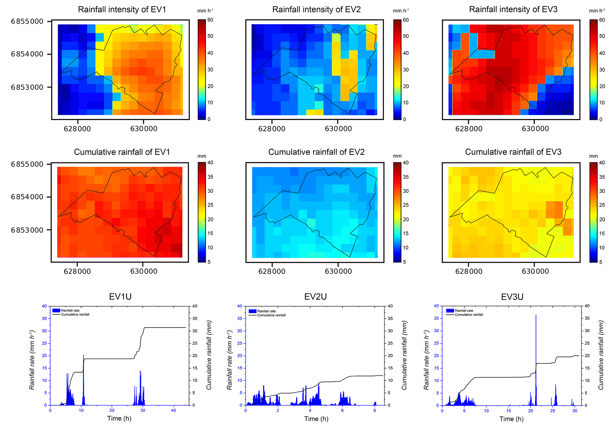
Figure 3The top row shows the rainfall intensity at the largest rainfall peak (per radar pixel) over the Guyancourt catchment area for the three studied rainfall events, the middle row shows the cumulative rainfall depths (per radar pixel) over the Guyancourt catchment area for the three studied rainfall events, and the bottom row shows the time evolution of rainfall rate (millimetres per hour) and cumulative rainfall (millimetres) of the three uniform rainfall events over the whole catchment.
The three uniform rainfall events (EV1U, EV2U, and EV3U) were constructed by spatial averaging over the whole catchment of originally distributed rainfall fields at each time step. Figure 3 (bottom) presents the time evolution of the corresponding rainfall rates and cumulative rainfall depths. Each of these events is sufficiently long to contain several rainfall peaks and dry periods. For EV1U, the highest rainfall intensity reaches 20 mm h−1, and the total rainfall accumulates (around 31.5 mm) fast between the first and the third rainfall periods (approximately 24 h). The maximum rainfall intensity of the EV2U and EV3U is 9 and 36.4 mm h−1, and the total rainfall amounts about 12 and 20 mm, respectively. Although the largest rainfall peak of the EV3U is 36.4 mm h−1, it lasted only for 3 min, just sufficient enough to contribute about 10 % to the total rainfall depths.
Overall, this initial analysis suggests that, in spite of some similar characteristics, the selected events cover a truly wide spectrum of rainfall space–time variability. However, to deepen the knowledge of intersection effects between the spatial variability in rainfall and spatial distribution of NBSs, we also considered four synthetic rainfall events (EV4–EV7). All these events are based on the EV3U, by selecting the 2 h period with the highest rainfall peak around 35 mm h−1 (catchment averaged), as illustrated on Fig. 4a. However, in the 3 min duration of the largest rainfall peak of the EV3U, a new space distribution and/or intensity of the rainfall was imposed for each synthetic rainfall event. As shown in Fig. 4b, the catchment-averaged maximum rainfall peak is about 37 mm h−1 for the EV4, and the corresponding catchment-averaged cumulative rainfall is about 4 mm. During these 3 min, the rainfall was redistributed in a binary manner in space (Fig. 4c), with the maximum intensity around 55 mm h−1. For the remaining synthetic rain events, this binary distribution was modified as follows (see Fig. 4d–f): the same maximum intensity of 55 mm h−1 and zero rainfall elsewhere (EV5), the maximum intensity of 17 mm h−1 and zero rainfall elsewhere (EV6), and the maximum intensity of 55 mm h−1 has been replaced by zero rainfall (EV7).
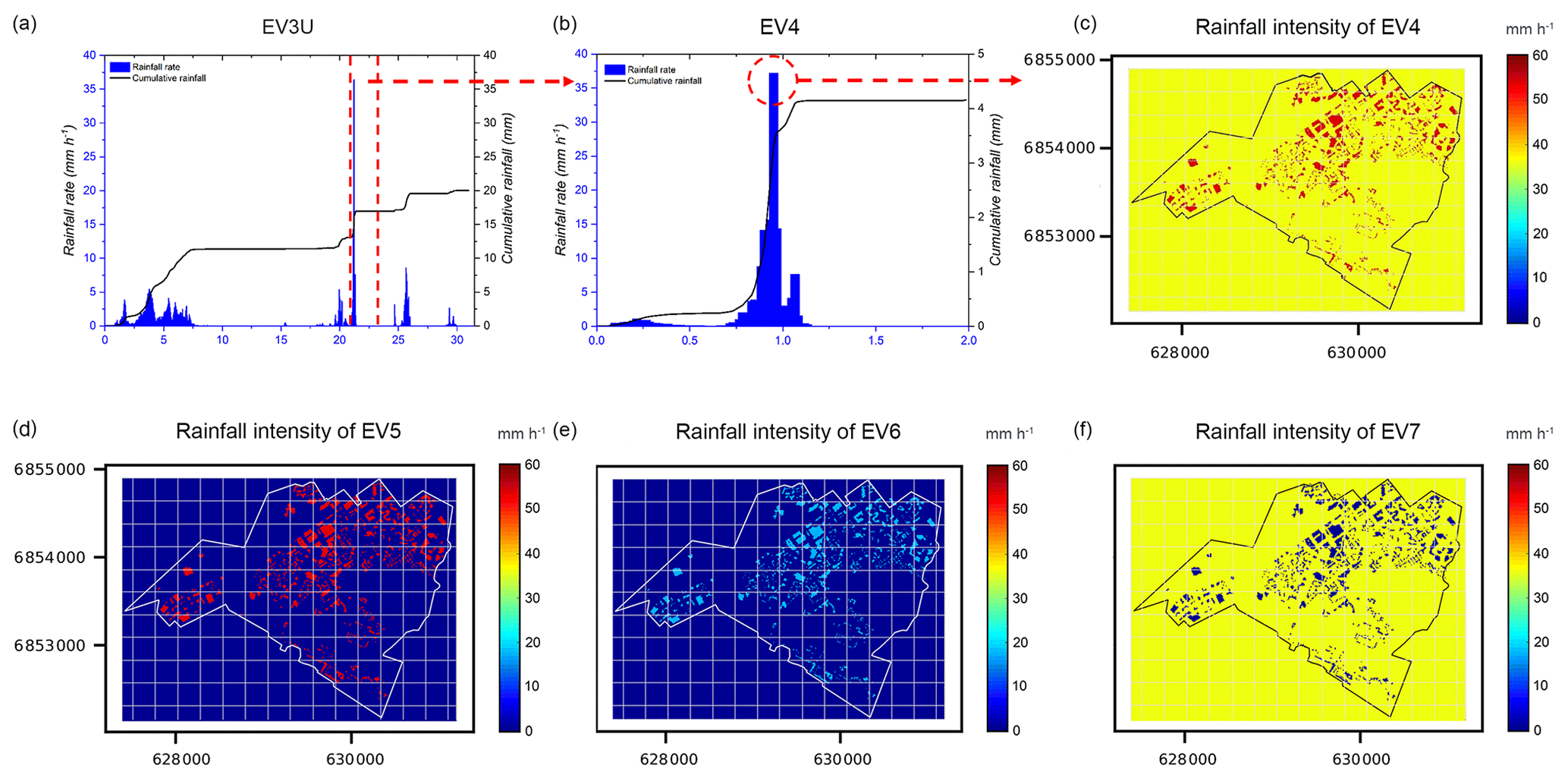
Figure 4(a) Time evolution of rainfall rate (millimetres per hour) and cumulative rainfall (millimetres) of the EV3U over the whole catchment (the period between the red dashed lines is the selected period for creating the EV4). (b) Time evolution of catchment-averaged rainfall rate and cumulative rainfall of the EV4 over the whole catchment. (c) The rainfall intensity at the largest rainfall peak (distributed) over the Guyancourt catchment for the EV4 (the red pixels are the location of green roofs (GRs) in GR1 scenario with the highest rainfall intensity in space), the rainfall of other areas are uniform. (d–f) The rainfall intensity at the largest rainfall peak (distributed) over the Guyancourt catchment for the EV5, EV6, and EV7, respectively.
2.3 Multi-Hydro model
The Multi-Hydro model is a fully distributed and physically based hydrological model, which has been developed by Hydrology Meteorology & Complexity Laboratory (HM&Co Lab) at ENPC (El Tabach et al., 2009; Giangola-Murzyn, 2013; Ichiba, 2016; Ichiba et al., 2018). It has been successfully implemented and validated in several catchments (e.g. Versini et al., 2016; Ichiba et al., 2018; Gires et al., 2017, 2018; Alves de Souza et al., 2018; Versini et al., 2018; Paz et al., 2019). In this study, it is used for assessing hydrological responses of the NBS scenarios at the urban catchment scale.
Multi-Hydro constitutes the interactive core among the four open-source modules (rainfall, surface, groundwater, and drainage) that represent the essential elements of the hydrological cycle in an urban environment.
The rainfall module (MHRC) can process different kinds of rainfall data (from radar or rain gauge). In order to adapt the rainfall inputs for Multi-Hydro, the intersection between the pixels of the model (with a 10 m spatial resolution in this study) and the pixels of the X-band radar data (with a 250 m spatial resolution) were performed by the QGIS (quantum GIS) interface using the following equation (Paz et al., 2018):
where is the rainfall rate computed on the model pixel of coordinates (iM,jM), and is the rainfall rate measured by the X-band radar on its pixel of coordinates (iX,jX). denotes the surface of any pixel S; in particular, is the surface of the model pixel (it does not depend on the coordinates but only on the model resolution).
The surface module (MHSC) of Multi-Hydro uses the code of the Two-Dimensional Runoff Erosion and Export (TREX) model that computes the interception, storage, and infiltration occurring at each pixel in terms of the properties of each land use (Velleux et al., 2008). The infiltration process of the surface module is governed by a simplification of the Green and Ampt equation (see p. 4 of the TREX user manual). The diffusive wave approximation of the Saint-Venant equations is used for calculating the overland flow, following the conservation of mass and momentum equations.
The groundwater recharge and solute transport (Riva et al., 2006; Mooers et al., 2018) are the other significant aspects of the hydrological cycle. The groundwater module (MHGC) is based on the Variably Saturated and 2-Dimensional Transport (VS2DT) model developed by the U.S. Geological Survey. This module can be used to simulate variably saturated transient water flow and solute transport in one or two dimensions (Lappala et al., 1987; Healy, 1990). The drainage module (MHDC) in Multi-Hydro uses the code of 1D SWMM model (James et al., 2010) to simulate the sewer network. This model represents the flow computed by 1D Saint-Venant equations in conduits and nodes.
In this study, we used the Multi-Hydro interaction between the surface module and the drainage module to focus on the rainfall–runoff modelling of NBS scenarios. In urban areas, groundwater can produce infiltration into the drainage pipes due to cracks in the structure (see Lucas and Sample, 2015, for an example). The absence of a long recession limb on the hydrographs indicates there are no such problems on the studied watershed. Groundwater can also eventually contribute to surface flooding when it is saturated. Such phenomenon did not occur on the studied area due to its pedology and the considered (not extreme) rainfall events. For these reasons, groundwater (as evapotranspiration) has not been considered in this study. That has been focused on the fast response of the watershed at the rainfall event scale.
The high spatial resolution of Multi-Hydro allows an easy implementation of small-scale controlled measures, like the rain garden, green roof, bio-retention swale, porous pavement, and rainwater tank, by locally modifying the land use parameters to link the size and shape of the corresponding NBS infrastructures with their infiltration and storage capacities.
3.1 Multi-Hydro implementation in the Guyancourt catchment
Based on the fully distributed character of Multi-Hydro, users can choose a specific spatial resolution. In this study, Multi-Hydro was implemented with a 10 m spatial resolution (the grid system creates square grids with a cell size of 10 m), and a temporal loop of 3 min. The 10 m resolution was performed because it sufficiently represents the heterogeneity of the catchment and also because it saves computation time.
Analogous with Eq. (1), the rainfall input for Multi-Hydro has been also time interpolated from the X-band radar measurements, as follows:
where Rm(j) is the rainfall rate during the jth time interval Δm(j) of the model, and Rr(i) is the rainfall rate during the ith time interval Δr(i) of the X-band radar. |Δ| denotes the length of any interval Δ, and δm=|Δm| is the length of any time interval of the model. Note that, while the duration of the time loop to generate the model outputs is 3 min (to keep it comparable with the X-band radar time interval), δm= 1 min for the rain input to Multi-Hydro.
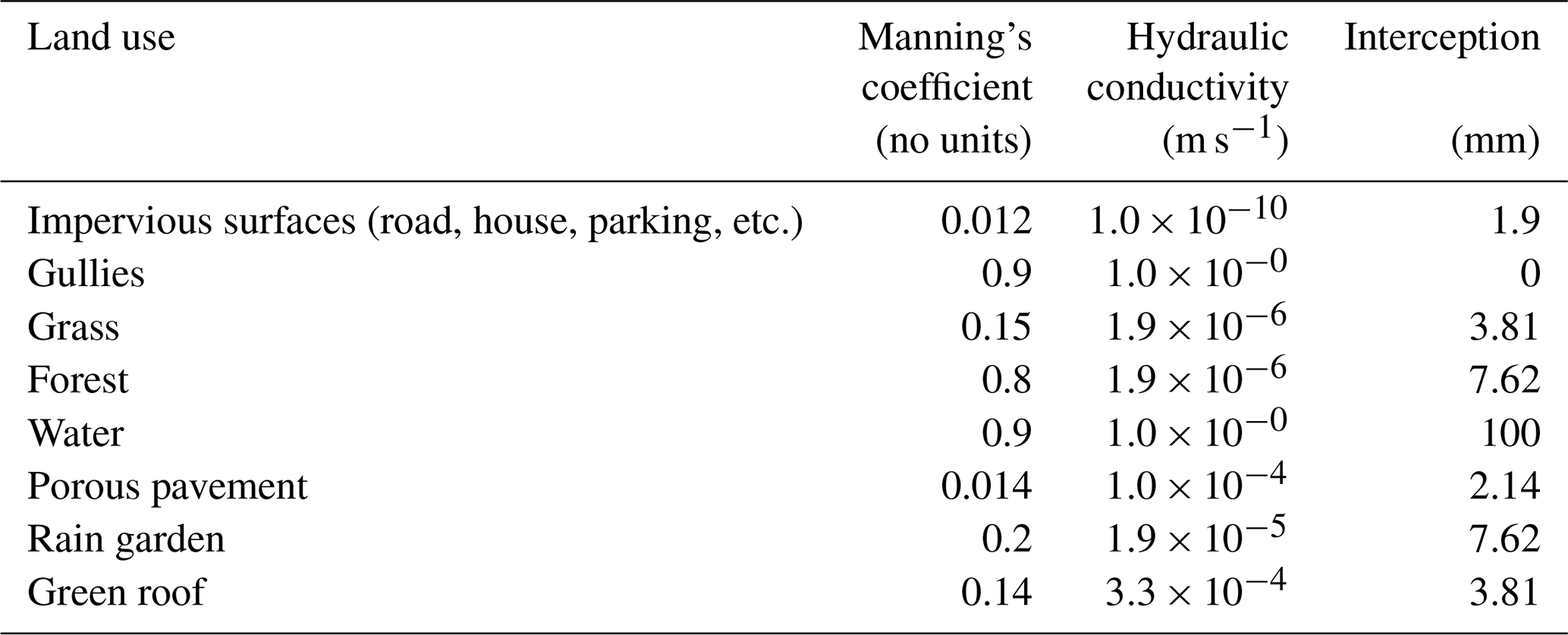
The implementation of Multi-Hydro in a new catchment starts with the conversion of the original GIS data (e.g. land use and topography) into the standard rasterized format with the desired resolution by using the MH-AssimTool (Richard et al., 2013), a supplementary GIS-based module for generating the input data for Multi-Hydro. During this process, a unique land use class was assigned to each pixel, specifying its hydrological and physical properties. In order to attribute a unique land use class to each pixel, the following priority order was used in this study: gully, road, parking, house, forest, grass, and water surface. For this study, all the standard model parameters related to the land use classification were selected from the Multi-Hydro manual (Giangola-Murzyn et al., 2014). The most important parameters are Manning's coefficient (no unit), hydraulic conductivity (metres per second) and interception (millimetres), as they are shown in Table 2. As already indicated, the Multi-Hydro does not use the traditional calibration of these parameters. If their most common values are always used, the reliable heterogeneity of the watershed for each case study is obtained by a rapid optimization of the spatio-temporal resolution of the model, with possibly refined classes of the land use and their orders (Ichiba et al., 2018).
Since the gully is actually the only land use class able to connect the surface module and the drainage module, it has the highest priority (i.e. if a raster pixel contains gully and the other land use classes do not, the whole pixel will be considered as gully). Generally, this order considers the impervious land use classes to have higher priority than the permeable land use classes, which results in an overestimation of impervious land uses (see Ichiba et al., 2018, for an alternative approach). After the rasterization process, the impervious land uses occupied 54 % of the Guyancourt catchment (Fig. 5). Besides the land use, the elevation was also assigned to each pixel of the model. For this purpose, the interpolation method was used to downscale the raw DEM data from 25 to 10 m (DEM25–10) to incorporate it with the model resolution. More precisely, each pixel was first subdivided into 25 equal sub-pixels as a proxy of the 5 m resolution, and then the elevation data were upscaled to 4 by 4 pixels to produce the 10 m interpolation of the original elevation.
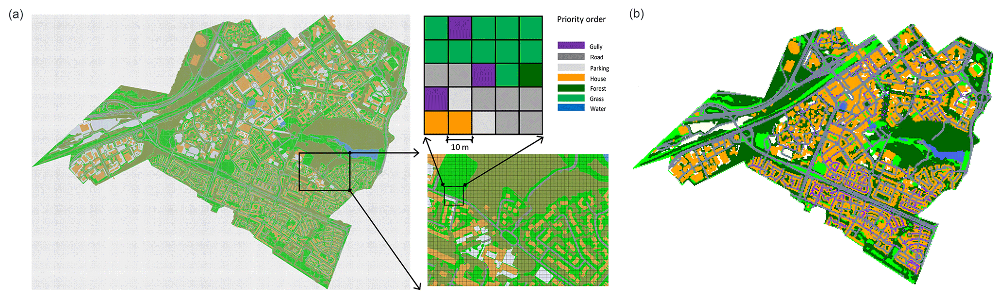
Figure 5(a) Rasterization of the original land use data into 10 m with priority order and (b) the rasterized land use data.
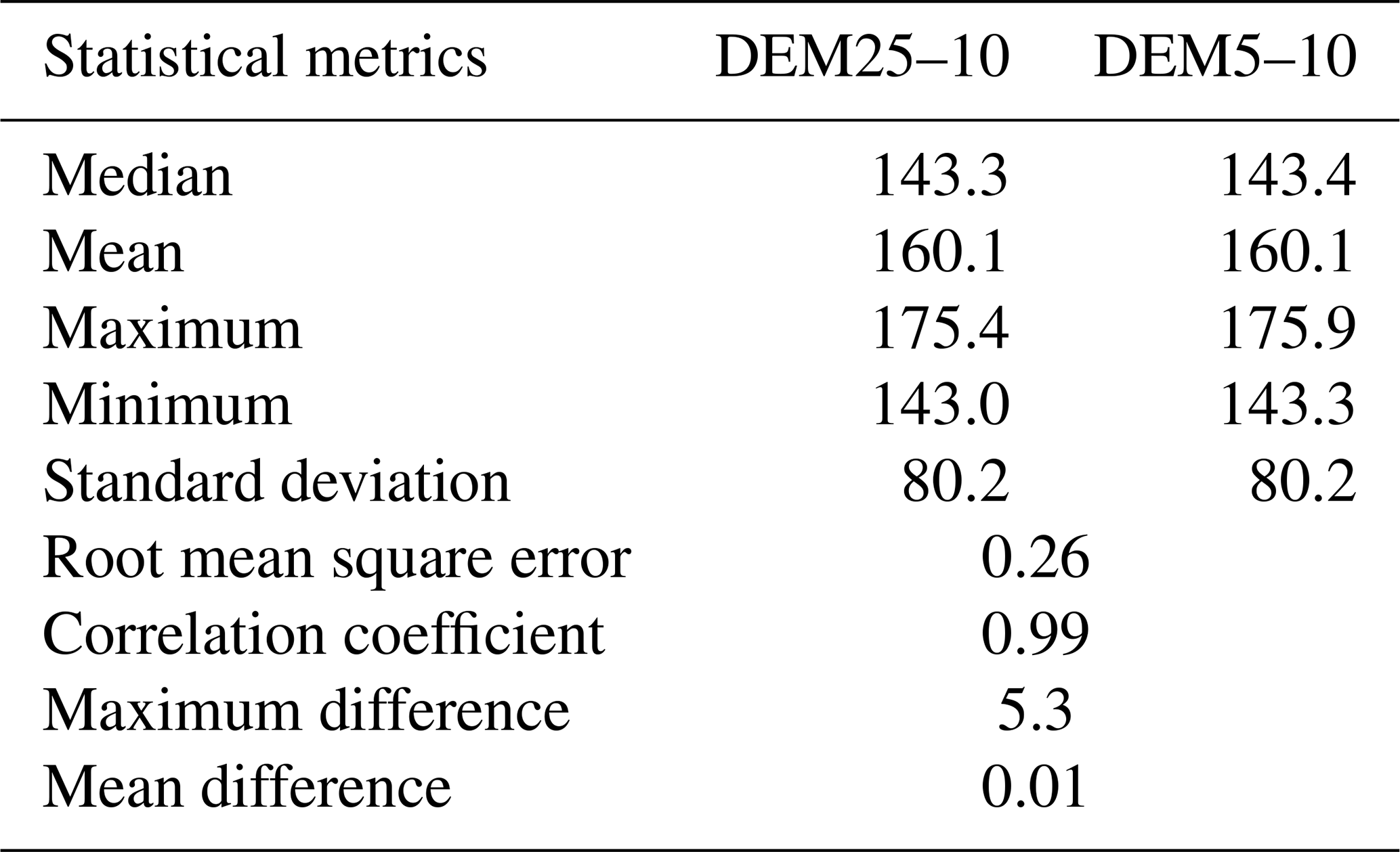
While the 25 m resolution DEM may seem too coarse to use for an urban area, it did not limit the study in any way because the catchment is relatively flat. To test this, we upscaled the raw 5 m DEM data to adapt them to the model resolution (DEM5–10). Table 3 presents the results of the statistical analysis of DEM25–10 and DEM5–10, which are so similar that the difference could not impact the results. For instance, the root mean square error is about 0.26, and the correlation coefficient is around 0.99. Besides, the ensemble of the data actually available for the Guyancourt watershed would need to be more detailed to make it worth going to a higher resolution of the model.
As the most considered NBSs correspond to more specific land uses, they are characterized with different retention capacities, and the related parameters are based on the literature (Dussaillant et al., 2004; Kuang et al., 2011; Park et al., 2014). To be more specific, the rain gardens (RGs) are characterized with the depression depth of 0.3 m. Thus, the storage capacity of RGs is about 300 L m−2. For the porous pavements (PPs), the thickness of the pavements is 0.21 m (pavement – 0.08 m; bedding material – 0.03 m; base material – 0.1 m). The porosity of pavement, bedding material, and base material is 5.4 %, 28.29 %, and 22.66 %, respectively. This indicates that the storage capacity of PPs is approximately 74 L m−2 in this study. For these two NBS measures, a simple procedure represents both the infiltration and storage processes that have been carried out. For each time step, if the rainfall rate is lower than infiltration rate of the PP or RG, the water is stored. If not, then ponding occurs.
Green roof is a special NBS measure that can be simulated by a specific module in Multi-Hydro (Versini et al., 2016). Accordingly, five physically based parameters are defined for the green roof. They are based on the experimental site of Cerema (Ile-de-France) where several green roof configurations were monitored (see Versini et al., 2016). In detail, the chosen configuration is the following: substrate thinness of 0.03 m and characterized by a porosity of 39.5 %, an initial moisture condition of 10 %, a field capacity of 0.3, and a hydraulic conductivity of 1.2 m h−1.
3.2 Simulation scenarios
To achieve the purpose of the study, a series of NBS scenarios were created and simulated for both rainfall inputs (described in Sect. 2.2). The baseline scenario is considered as being the current configuration of the Guyancourt catchment, without implementing any NBSs (Fig. 2; left). The baseline scenario will be used later on for the model validation.
The first set of NBS scenarios includes porous pavement (PP1), rain garden (RG1), green roof (GR1), and their combined scenario (Combined1). They are applied to assess the impacts of the spatial variability in rainfall on the hydrological responses of NBS scenarios. For each scenario, the corresponding NBSs are implemented heterogeneously over the catchment, while respecting the local catchment conditions and storm water management requirements. For instance, with the help of the detailed land use GIS data, we initially selected all the buildings having flat roofs, and then these impervious roofs were converted into green roofs for the GR1 scenarios by adapting the land use data.
The second set of NBS scenarios (PP2, RG2, GR2, and Combined2) was proposed with a different arrangement to assess the potential effects of a heterogeneous implementation of NBSs at the urban catchment scale. For each pair of scenarios with a given type of NBSs, their implementation occupies the same percentage of the space over the whole catchment but differs significantly in terms of spatial distributions of the considered asset. Considering now the roofs with certain slopes (≤ 15∘), they can be also used to implement green roofs (Stanić et al., 2019). The impervious roofs that satisfied this condition were converted into small and light green roofs and used for the GR2 scenario. While the two scenarios (GR1 and GR2) occupy the same percentage of the whole catchment, their density is different simply because of the difference in original densities of the buildings. The designing process for other NBS scenarios follows a somewhat similar logic. All details concerning the scenarios of the NBS implementations, including a detailed description of each NBSs and the percentage of the space required for its implementation at 10 m resolution, are presented in Table 4, while the maps of the resulting land use are illustrated in Fig. 6.
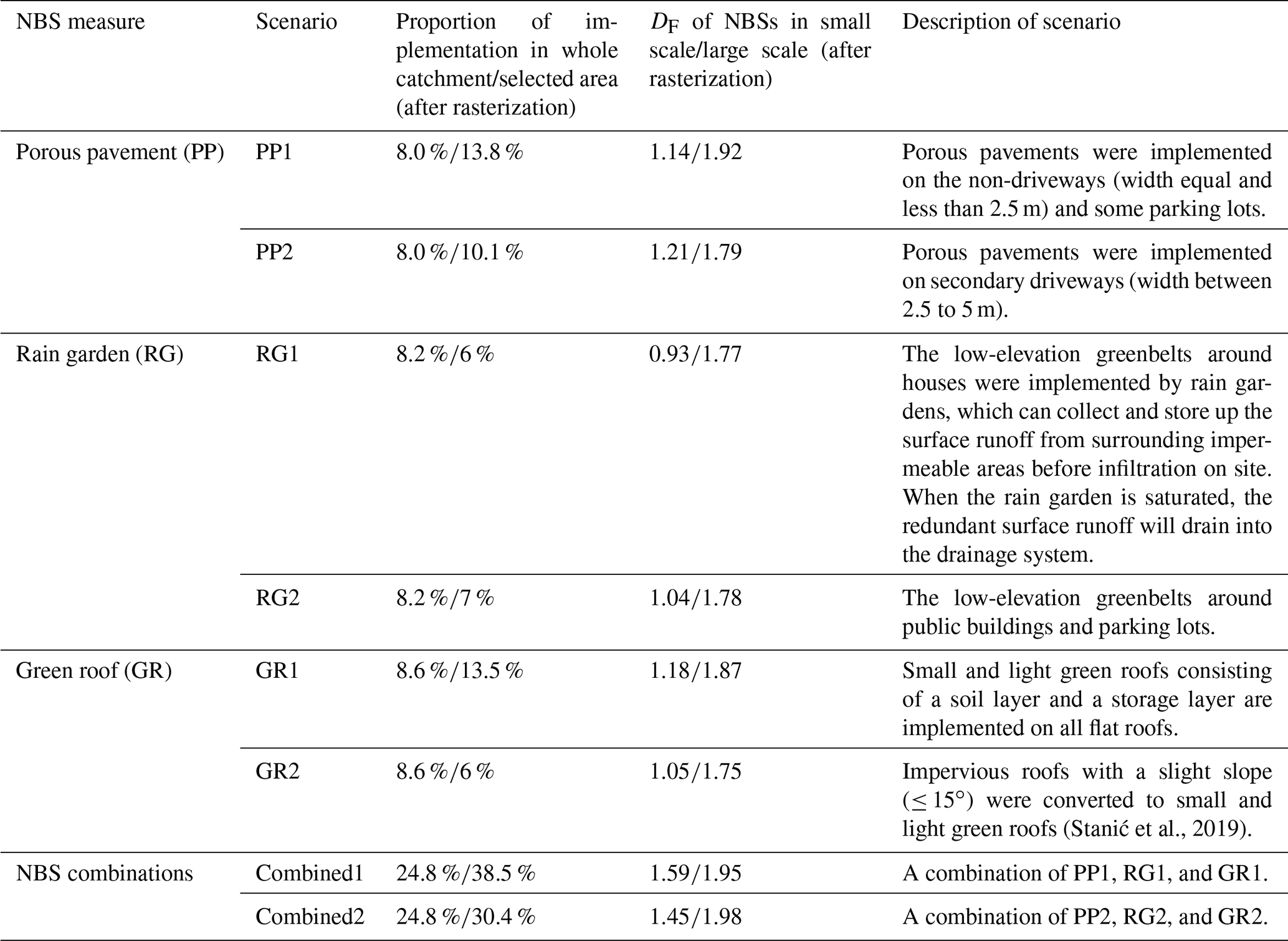
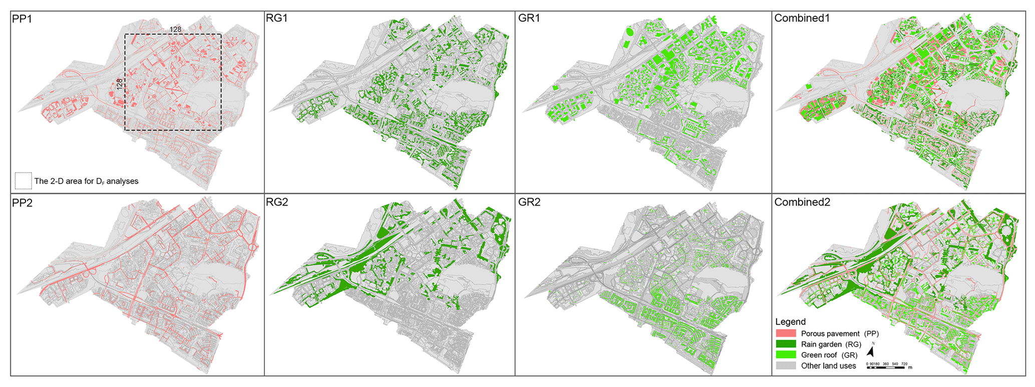
Figure 6A total of two scenarios for each of NBS implementation, including porous pavement (PP1 and PP2), rain garden (RG1 and RG2), green roof (GR1 and GR2), and Combined1 and Combined2. The rectangular area in the PP1 scenario is the example area for applying fractal analysis.
Table 4 provides also the estimates of the scale-independent indicator, discussed in detail in the following sections, called the fractal dimension. To obtain it intuitively, this indicator for the two combined scenarios (Combined1 and Combined2) is close to 2 over the range of large scales of the 2-dimensional space. This indicates that NBSs are rather homogeneously implemented over the whole catchment. However, it is important to note that, in spite of the initially identical percentage that has been used to characterize the implementation of the NBS pairs over the catchment at a 10 m scale, the resulting fractal dimension could be quite different. It is simply because the percentage of the space required for the NBS implementation remains a scale-dependent quantity, i.e. it depends on the resolution of the model, while the fractal dimension quantifies the propagation of the spatial heterogeneity for each of NBS scenarios, from the smallest scale to the outer scale of the catchment. This propagation remains scenario dependent only and, hence, subject to its optimization.
3.2.1 Fractal dimension of NBS scenarios
To quantify the multiscale space heterogeneity of NBSs in each NBS scenario, we applied the concept of fractal dimension (DF), which was initially introduced to describe the scale invariance of some irregular geometric objects (Mandelbrot, 1983), namely a similar structure can be observed at any scale. DF has been often used in catchment hydrology (e.g. Schertzer and Lovejoy, 1984, 1987, 1991; Lavallée et al., 1993; Gires et al., 2013, 2017; Ichiba et al., 2018; Paz et al., 2020; Versini et al., 2020). In this study, a standard box-counting technique was applied to estimate the DF of each NBS scenario (Hentschel and Procaccia, 1983; Lovejoy et al., 1987). The DF of a geometrical set A (here represented by the non-overlapping pixels of NBSs embedded in a 2-dimensional space) is obtained with the following power law:
where Nλ,A is the number of non-empty (containing NBSs) pixels to cover the set A, at the resolution λ , which is defined as the ratio between the outer scale L and the observation scale l (. The symbol ≈ means an asymptotic relation (i.e. for large resolution λ and possibly up to a proportionality prefactor).
Based on Eq. (3), we count the number of pixels containing at least one NBS by starting with the smallest pixel size (l= 10 m in this study) and then continuously increasing the pixel size by simply merging the four adjoining pixels. This procedure is repeated until reaching the largest pixel size (L). Thus, Nλ,A is counted at different resolutions, and the results are plotted in the log–log plot (see Fig. 7). Corresponding to Eq. (3), the fractal dimension DF of each NBS scenario is defined as follows:
Here, for each scenario, a square area of 128×128 pixels was extracted from the catchment to make the fractal analysis (see the example of the PP1 scenario in Fig. 6). In order to avoid the no data areas, which would bias the fractal dimension estimate, the selected square area is the greatest possible size characterized by a multiple of two in the studied catchment.
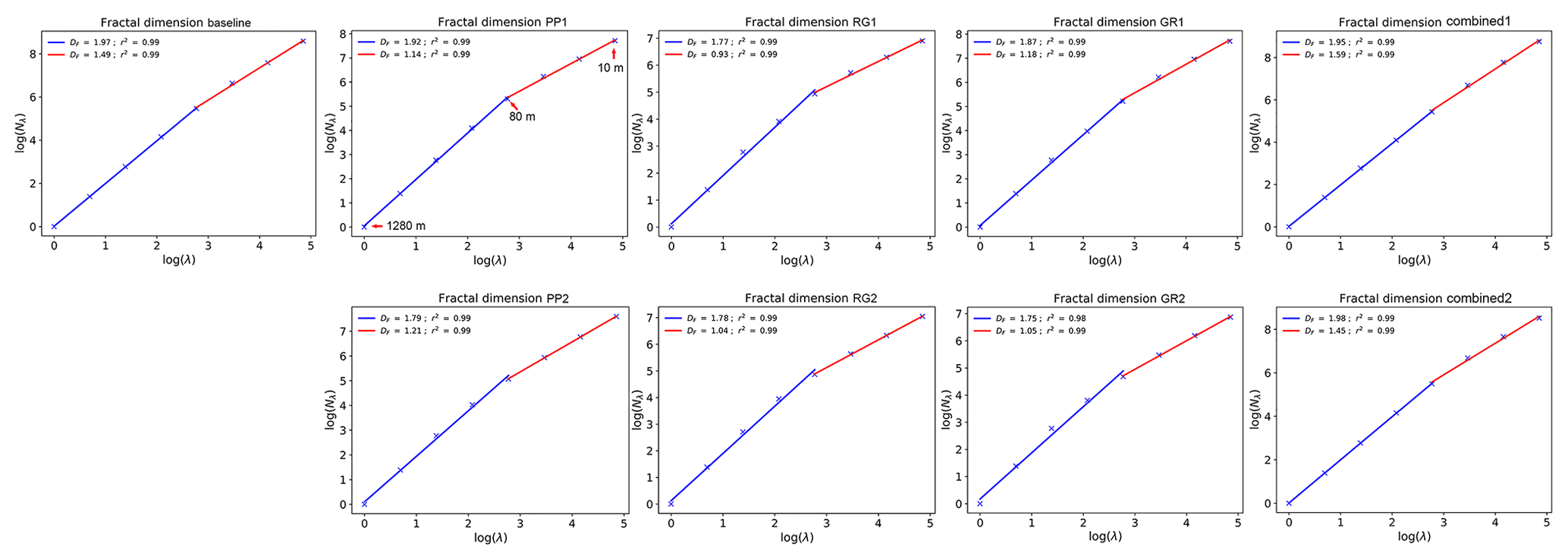
Figure 7The fractal dimension of impervious surface of the baseline scenario and the fractal dimension of NBSs in each NBS scenario.
As shown in Fig. 7, all the NBS scenarios are presented with two scaling behaviour regimes, with a scale break roughly at 80 m. For each regime, the scaling is robust, with linear regression coefficients (R2) around 0.99. For the first regime corresponding to the small-scale range (10–80 m) that related to the asset implementation level, the dimension DF is around 1 for most of NBS scenarios. It is in contrast with the second regime, the large-scale range (from 80 to 1280 m) that exhibits a scaling behaviour with a DF ranging from about 1.75 to 1.98. We also applied fractal analysis on the impervious surface of the baseline scenario in the same selected area, and we also found the same scale break at 80 m (the DF of the baseline scenario in each regime are presented in Fig. 7). Therefore, it rather confirms that the spatial distribution of NBSs is strongly constrained by the urbanization level of the catchment.
3.2.2 Multifractal intersection theorem
We would now like to illustrate and emphasize why it is so indispensable to take into account the multiscale space variability in both the rainfall and the NBS distribution. For instance, both hot spots (extremes) of the rainfall and NBSs are scarce and, therefore, could rarely coincide, i.e. rainfall spikes may fall more often elsewhere than on NBSs. Similar questions can occur for less extreme events. The effective NBS performance could be, therefore, biased with respect to their potential performance due to this problem of intersection between rainfall intensity and NBSs. It reminds us of the so-called multifractal intersection theorem applied to the intersection of a rainfall with extreme space variability and a rain gauge network that provides quantitative estimates of this intersection (Tchiguirinskaia et al., 2004). Figure 8, adapted from this paper, schematically represents the intersection at a given time of a (multifractal) rainfall, displaying quite variable pixel intensities ranging from light blue to dark brown (e.g. from 1 to 100 mm h−1), with a heterogeneous rain gauge network (light brown pixels). The resulting measured rainfall field M is simply the product of the rainfall intensities R by the gauge characteristic function N (= 1 if there is a gauge in this pixel; otherwise, it is 0). The intersection theorem states that, for fractal objects like for the usual (Euclidean) geometric ones, the codimension – i.e. the complement of the dimension DM to the embedding space dimension d– of the measured field above a given intensity threshold is the sum of the codimensions of the network ( and of the real field ( above the same intensity threshold, as follows:
For instance, the intersection in a plane (d=2) of two straight lines ( corresponds to a point (cM=2, DM=0). Of particular interest is the case where the intersection is so small that its codimension cM is larger than the embedding dimension d, i.e. has a negative dimension DM (Schertzer and Lovejoy, 1987). Due to Eq.(5), the codimension of the network cN is thus the critical dimension of the (real) field under which the rainfall intensity is rarely measured by the network, as follows:
More precisely, the smaller DR is with respect to cN, the lesser extent to which the real field R is measured. Let us mention that Paz et al. (2020) used this intersection theorem to determine when the adjustment of radar data by a rain gauge network becomes misleading instead of improving the data.
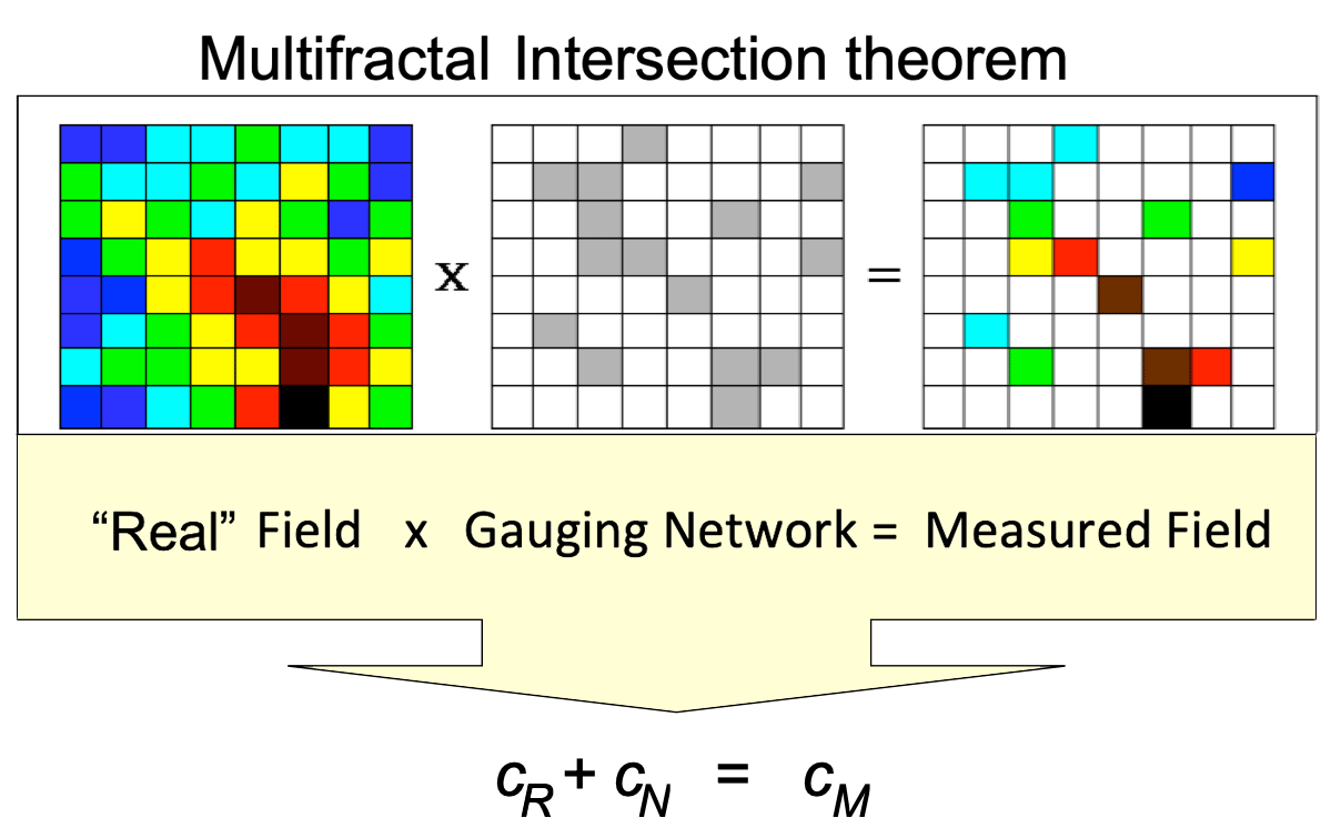
Figure 8Schematic of the (multifractal) intersection theorem applied to the measured rainfall M by a rain gauge network N. The measured rainfall corresponds to the product of the real rainfall R by the gauge characteristic function (= 1 if there is a gauge in this pixel; otherwise, it is 0) and the corresponding codimensions and are added to yield the codimension of the measured rainfall . d is the embedding space dimension, and DR, DN and DM are the corresponding fractal dimensions (adapted from Tchiguirinskaia et al., 2004).
The assessment of the performance of an NBS network cannot be reduced to the binary question of the presence of an NBS or not, like done for a rain gauge of a network. However, we can immediately state that they will be more and more ineffective for rainfall intensity for which the fractal dimension is more and more below the codimension cN of the network. This is already an important piece of information that can be used to design NBSs and their networks. This also explains why we estimated, in the previous subsection, the fractal (co-)dimension of the NBS network and compared, in Sect. 4.3, the simulations resulting from spatially uniform rainfall (DR=d, cR=0) and spatially heterogeneous rainfall (DR<d, cR>0).
3.3 Modelling experiments
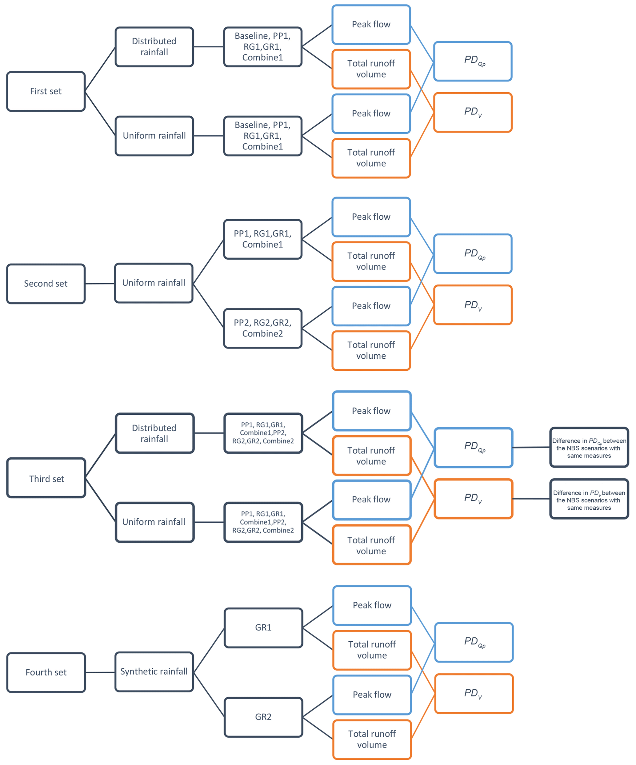
The overall target of the study is to investigate whether the spatial variability in rainfall and the spatial arrangement of NBSs have an impact on the hydrological responses of NBS scenarios at the urban catchment scale. For this purpose, four sets of modelling experiments were prepared, and two indicators (PD – percentage difference in peak flow; PDV – percentage difference in total runoff volume) were used to quantify the uncertainty associated to rainfall and NBS spatial distribution in the hydrological response of the catchment. Figure 9 presents the flow chart of the four sets of modelling experiments. In addition, the corresponding descriptions are presented as follows:
-
The first set is used to investigate the impact of spatial variability in rainfall on the hydrological responses of NBS scenarios. In this first set, we employed the following scenarios: baseline, PP1, RG1, GR1, and Combined1. These five scenarios were simulated under the distributed and uniform rainfall inputs. Then, we computed the ratio of peak flow (Eq. 7) and the PD and PDV indicators (Eqs. 8 and 9) for each scenario under two different kinds of rainfall inputs.
-
The second set is used to analyse the impact of the spatial distribution of NBSs on the hydrological responses of the NBS scenarios. In this experiment, we compared the two groups of NBS scenarios mentioned in the Sect. 3.2 (GR1 vs. GR2, for instance). The eight scenarios were simulated only with the uniform rainfall in order to avoid the impact of spatial variability in rainfall and to focus on the uncertainty associated with the spatial arrangement of NBSs.
-
The third set is used to analyse the intersection impact of spatial variability in rainfall and the spatial distribution of NBSs on the hydrological responses of the catchment. In this experiment, the eight mentioned NBS scenarios were simulated under the distributed and uniform rainfall, respectively. Then, the PD and PDV of each NBS scenario were computed by comparing the results obtained for the two different kinds of rainfall inputs (distributed and uniform). Then, we compared the difference in PD and the difference in PDV between the NBS scenarios characterized by the same solutions or measures.
-
The fourth set is to verify the generality of the results obtained; we extended the study of hydrological responses to the intersection of the distributed rainfall and NBSs by applying the synthetic rainfall events of EV4–EV7 in two green roof scenarios (GR1 and GR2). The reason is the difference in DF between GR1 and GR2 is larger compare to the other NBS scenarios. Thus, the intersection effects can be more significant for these two scenarios. Here, the GR1 scenario was taken as the reference scenario, assuming that the extremes of rainfall (hot spots) only fall on the GRs of the GR1 scenario. With this respect, the rainfall was redistributed in a binary manner in space during the 3 min that lasted at the largest rainfall peak of the EV3U, as illustrated on Fig. 4c-f. Namely, the hot spots of the EV4–EV6 are strictly intersected with the distributions of GRs in GR1, while the GR2 scenario is not. Contrary to EV4–EV6, EV7 corresponds to the no rain situation on GR1 during the same 3 min.
The peak flow ratio and the two indicators are especially calculated for the sum of four highlighted conduits connected to the catchment outlet (the right side of Fig. 2) with the following equations:
where and refer to the peak flow of scenarios under the distributed rainfall and uniform rainfall, respectively, for the first and third modelling experiment. For the second experiment, they represent the peak flow of the first set of NBS scenarios and the second set of NBS scenarios, respectively. For the fourth set experiment, they represent the peak flow of the GR1 and GR2 scenarios, respectively. Correspondingly, for the first and third modelling experiments, V1 and V2 refer to the total runoff volume of scenarios under the distributed rainfall and uniform rainfall, respectively. For the second modelling experiment, they represent the total runoff volume of the first set of NBS scenarios and the second set of NBS scenarios, respectively. For the fourth set experiment, they represent the total runoff volume of the GR1 and GR2 scenarios, respectively.
3.4 Model validation
Before the simulation of the NBS scenarios, Multi-Hydro was validated with the water levels of the storage basin by applying the baseline scenario under the three distributed rainfall events. The simulations were then repeated with the three uniform rainfall events, respectively. The model performance was evaluated through two indicators, namely the Nash–Sutcliffe Efficiency (NSE) and percentage error (PE). The Nash–Sutcliffe Efficiency (NSE ≤ 1) is an indicator generally used to verify the quality of the hydrological model simulation results, described as follows (Nash and Sutcliffe, 1970):
where Si refers to simulated values, Oi refers to observed values, and represents the average of the observed values. The NSE closer to 1 indicates that the model is more reliable, whereas an NSE closer to 0 indicates that the simulation does not better than that of the average observed value , which means the simulation performance is rather poor. If the NSE is far below 0, it means the simulation is even worse performing than .
The percentage error (PE) represents the difference between observed values and simulation values, which reflects the reliability of the simulation values.
The values obtained for these two indicators are summarized in Table 5. They confirm that Multi-Hydro performs well for the case study area in the baseline scenario, suggesting that the model is reliable enough to study the impacts of spatial variability, either precipitation and/or NBS arrangements, on the hydrological responses under various NBS scenarios.
Table 5The NSE coefficients and PE values of baseline scenario under the three distributed rainfall events and three uniform rainfall events.
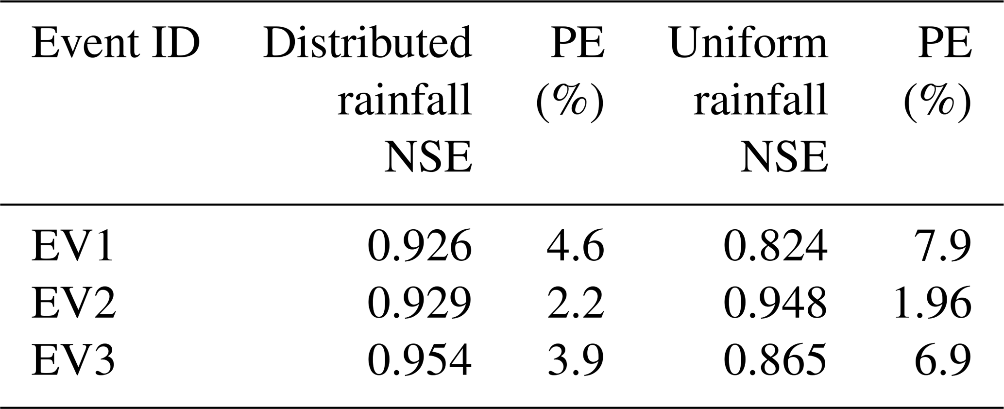
4.1 Validation of the baseline scenario
Regarding the observed and simulated water levels in the baseline scenario, the model indeed performs well for the studied area. The NSE coefficients and the PE indicators validated Multi-Hydro's performance (see Table 5). For the three distributed rainfall events (Fig. 10), the NSE coefficients are larger than 0.9, and PE indicators are lower than 5 %. For the uniform rainfall event of EV2U, the model represents the water levels with NSE equal to 0.95, and PE equal to 1.96 %; only a slight overestimation of the observed water levels is observed between hours 4 and 7. For the uniform rainfall of EV1U and EV3U, the temporal evolutions of simulated water levels slightly underestimate the observed ones, with NSE around 0.8 and PE around 7 %. Regarding the temporal evolutions of simulated water levels under the distributed rainfall of EV1 and EV3, they are more consistent with the observed ones. The reason is that the rainfall intensities of the distributed rainfall are generally higher than those of the uniform rainfall at the storage basin location. Namely, in the uniform rainfall events, the accumulated water levels in the storage basin are less than that of in distributed rainfall events. Overall, the distributed rainfall gives slightly better results, and the simulated water levels using uniform rainfall also match the observed ones sufficiently well to validate the Multi-Hydro implementation in the Guyancourt catchment.
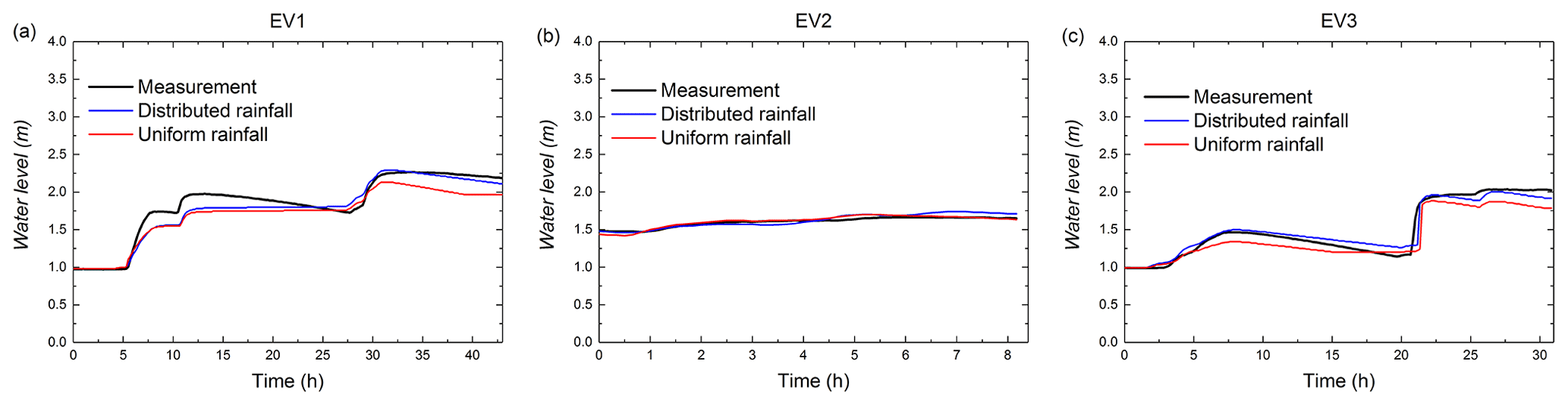
Figure 10Comparison of the observed and simulated water levels (simulated with distributed rainfall and uniform rainfall) of the three rainfall events, namely (a) EV1, (b) EV2, and (c) EV3.
Regarding the validation results, the scalability of Multi-Hydro allowed us to define the optimal resolution to finely reproduce the spatial heterogeneity of the watershed. Remember that this resolution is the ratio between the external scale of the watershed and the scale of the grid. The heterogeneity mentioned above propagates from the smallest scale to the largest, impacting the simulation results in any scale through the hierarchy of spatial scales of the watershed. It should be understood that the selected 10 m grid scale is not the smallest scale possible but the optimal one to ensure a good balance between, for example, sufficient heterogeneity and the required quantity of the data required, a gain in precision, and involved computing time. As discussed in Sect. 3.2, the spatial heterogeneity for each of the NBS scenarios evolves with the fractal dimension on two scale ranges, namely the asset implementation scales (10–80 m) and the larger basin scales. Such an evolution remains fully compatible with the intrinsic scalability of Multi-Hydro, which makes it particularly suitable and sufficiently reliable for studying the impacts of the spatial variability in hydrological responses in different NBS scenarios.
4.2 Impacts of spatial variability in rainfall
The impact of spatial variability in rainfall on the hydrological responses of each NBS scenario over the whole catchment was evaluated at the catchment scale in terms of the sum of flow in four conduits (highlighted on the right side of Fig. 2). These four conduits are chosen because they collect the runoff from the whole catchment and finally merge into the storage unit representing the outlet of the drainage system. To be more specific, the percentage difference in peak flow (PD and percentage difference in total runoff volume (PDV) computed for the first set of modelling experiments (described in Sect. 3.3) are presented in the following section.
4.2.1 Baseline scenario
Before continuing, it is important to assess the baseline scenario under both distributed and uniform rainfall by using the simulations already performed to validate the Multi-Hydro implementation in the Guyancourt catchment. As shown in the hydrographs (Fig. 11), the higher peak flow was generated by the distributed rainfall in EV1 and EV2. Hence, the peak flow ratio computed by comparing the distributed rainfall and uniform rainfall is larger than 1 (see the first column of Fig. 13a), but this ratio is around 0.9 in EV3. The reason is that, during the largest rainfall peak of EV1 and EV2, the rainfall intensity of all radar pixels in distributed rainfall is higher than those of uniform rainfall, while in EV3 the rainfall intensity of around 30 % radar pixels in uniform rainfall is about 28 mm h−1 higher than that of the distributed rainfall.
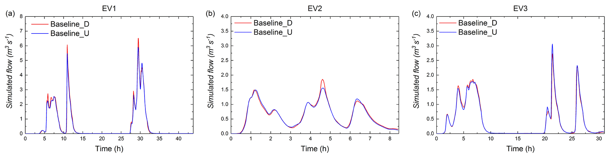
Figure 11Simulated flow (cubic metres per second) of the baseline scenario under three distributed rainfall events and three uniform rainfall events, namely (a) EV1, (b) EV2, and (c) EV3.
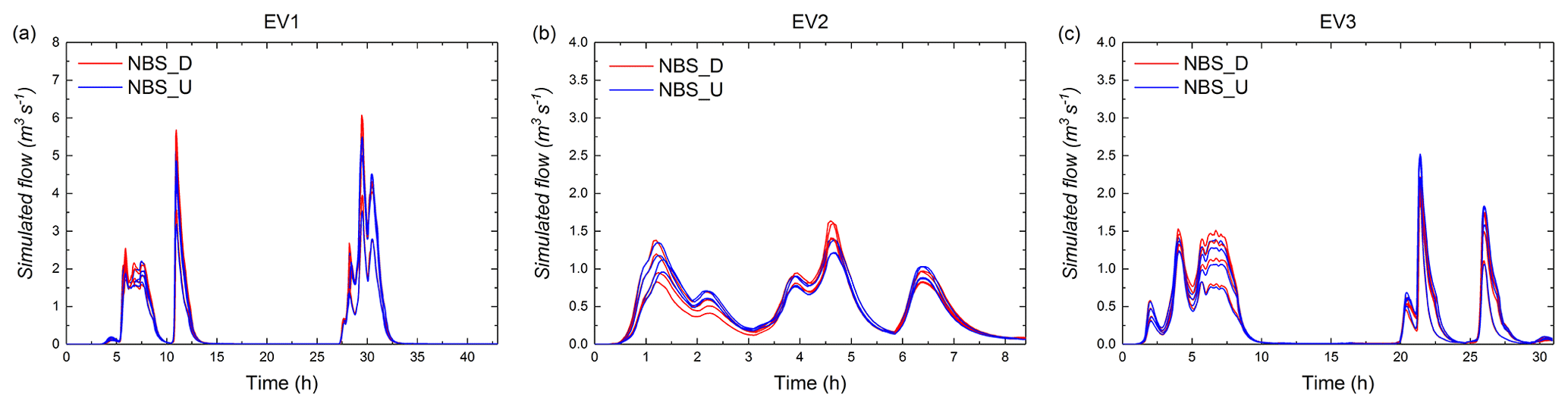
Figure 12Simulated flow (cubic metres per second) of the first set of NBS scenarios under three distributed rainfall events and three uniform rainfall events (the red hydrographs represent the NBS scenarios simulated with distributed rainfall, and the blue hydrographs represent the NBS scenarios simulated with uniform rainfall), namely (a) EV1, (b) EV2, and (c) EV3.
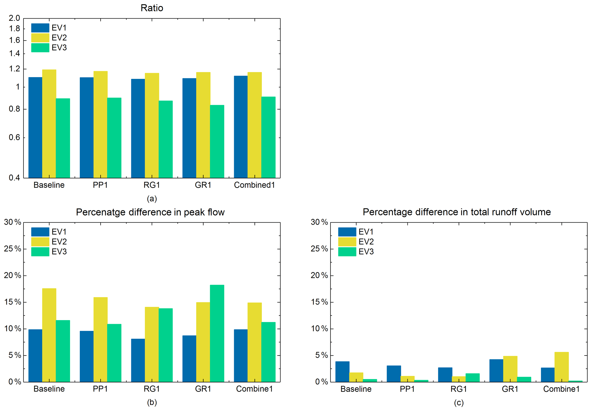
Figure 13(a) The ratio of peak flow between the scenarios under the distributed rainfall and the scenarios under the uniform rainfall. (b) Percentage difference in peak flow of the baseline scenario and the first set of NBS scenarios under the three distributed rainfall events and the three uniform rainfall events. (c) Percentage difference in total runoff volume of the baseline scenario and the first set of NBS scenarios under the three distributed rainfall events and the three uniform rainfall events.
As shown in Fig. 13b, the PD of baseline scenario in EV1, EV2, and EV3 is about 10 %, 17.6 %, and 11.6 %, respectively. According to the SD of the rainfall intensity at the largest rainfall peak of each event (Table 1), the spatial variability in the rainfall intensity of EV2 is more pronounced than that of EV1 and EV3. Accordingly, the PD of baseline scenario in EV2 is the highest. Regarding the total runoff volume (Fig. 13c), the PDV of the baseline scenario for the three rainfall events ranges from 1 % to 3.8 %. Contrary to the PD, the PDV of the baseline scenario is not correlated to the SD of the total rainfall depth. For the baseline scenario, it is noticed that the PD is more pronounced than PDV for all rainfall events. These results can be explained by the fact that the spatial variability in rainfall intensity at the largest rainfall peak is strong in all three rainfall events, while the total rainfall volume for the distributed and uniform rainfall inputs is the same. This small PDV is influenced by the differences in the grid scale (storage capacity, infiltration, etc.), which are differently modelled when the input is uniform or non-uniform.
4.2.2 NBS scenarios
In comparison to Fig. 11, Fig. 12 presents the simulated flow of the first set of NBS scenarios under the three distributed rainfall and three uniform rainfall events. The results remain consistent overall with the results in the baseline scenario. Indeed, as shown in Fig. 13a, the peak flow ratios between distributed rainfall and uniform rainfall simulations for the four NBS scenarios are larger than 1 for EV1 and EV2 and around 0.8 for EV3. The reason mentioned in the previous section.
As shown in Fig. 13b, the results of PD for PP1, RG1, and Combined1 scenarios are also consistent with the baseline scenario; PD is the lowest for EV1 and the highest for EV2. For these three NBS scenarios, PD ranges from about 8 % to 18 % for the three rainfall events. The relationship between the SD of the rainfall intensity at the largest rainfall peak and the PD of each NBS scenario (Fig. 14a) shows that PD (the uncertainty related to the peak flow) computed for PP1, RG1, and Combined1 scenarios increase simultaneously with the increase in the SD of the rainfall intensity. The results computed for GR1 scenario do not depict the same tendency; PD computed for EV3 is higher than those computed for the two other events. The reason is related to various factors. Namely, it may be affected by the intersection effects of the spatial variability in rainfall and the spatial arrangement of green roofs in the catchment. The reason can be explained by the fact that, in the GR1 scenario, the green roofs are mainly implemented on the locations with high distributed rainfall intensities. As demonstrated by many previous studies (Qin et al., 2013; Palla et al., 2015; Ercolani et al., 2018), GRs are usually more effective for intense but short rainfall peaks. In the case of the GR1 scenario under the distributed rainfall of EV3, GR measures effectively stored more runoff than in the uniform rainfall during the main rainfall peak. This enlarges the variability in the hydrological response in terms of peak flow.
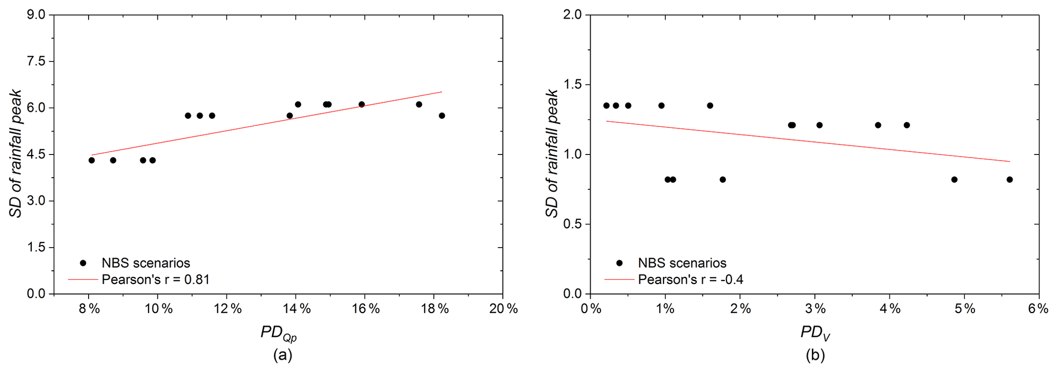
Figure 14(a) Relationship between the SD of rainfall intensity at the largest rainfall peak and PDQp of NBS scenarios. (b) Relationship between the SD of total rainfall depth and PDV of NBS scenarios.
Regarding the percentage difference in total runoff volume, it is noticed that the computed PDV are lower than 6 % for all NBS scenarios under the three rainfall events, especially in EV3, where they are lower than 2 % (Fig. 13c). Compared with the uncertainty of the peak flow, the resulting uncertainty of the total runoff volume is little influenced by the spatial variability in the rainfall. The reason is that the spatial variability in total rainfall depth is less pronounced with respect to the spatial variability in the rainfall intensity at the largest rainfall peak, and also, there is no highly localized storm cell in the studied events. Figure 3 (top) displays the rainfall intensity at the largest rainfall peak (per radar pixel) over the Guyancourt catchment for the three studied rainfall events. It is noticed that the highest rainfall peak of the distributed rainfall is very variable in space, which enlarges the discrepancy with the corresponding uniform rainfall, resulting in a significant impact on the peak flow of each NBS scenario that is simulated with two different rainfall inputs. However, the cumulative rainfall of the distributed rainfall input is not very variable in space (see Fig. 3; middle). For instance, the standard deviation (SD) of the cumulative rainfall of the three rainfall events is around 1 mm, which indicates that the spatial variability in the distributed rainfall is not very pronounced at most of the time steps. Thus, the difference between distributed rainfall and uniform rainfall is relatively small during the whole rainfall period. Finally, the simulated flow of NBS scenarios under two different rainfall inputs is similar in most time steps, resulting in the percentage difference in the total runoff volume of NBS scenarios (simulated by distributed rainfall and uniform rainfall) is not significant.
As illustrated in Fig. 14b, the relationship between the SD of total rainfall depth and the PDV of NBS scenarios is nonlinear. This can be explained by the fact that the three rainfall events are relatively long, and the hydrological performances of NBSs are gradually changed during the event (e.g. they can efficiently infiltrate or store water at the beginning and be saturated after a long rainfall period). Comparing the PDV of each NBS scenario for all three rainfall events (Fig. 13c), those computed for GR1 and Combined1 appear to be the highest for EV2. It could also be related to the intersection effects of spatial location of GR measures and the spatial variability in rainfall. Indeed, these GR measures (considered in the GR1 and Combined1 scenarios) are mainly located in the north side of the catchment. In this area, the first distributed precipitation of EV2 (1–3.5 h) is relatively weak and variable (i.e. there is no rainfall or the rainfall has very low intensity in some localization pixels). Furthermore, as the initial moisture condition of GR measures are considered as unsaturated in both distributed and uniform rainfall, the GR measures are more efficient at the beginning of the distributed rainfall than in the uniform rainfall and, finally, enlarge the uncertainty associated with precipitation variability (i.e. the corresponding PDV). More discussion about the intersection effects is presented in Sect. 4.3.
4.3 Impacts of the spatial distribution of NBSs
In order to analyse the impacts of the spatial distribution of NBSs on the hydrological responses of NBS scenarios, the results of the second set of modelling experiment (described in Sect. 3.3) are presented as follows. As shown in Fig. 15a, the PD of all NBS scenarios are lower than 5 %, and the PDV of all NBS scenarios are lower than 8 %, which indicates that the hydrological responses of NBS scenarios are little affected by the spatial distribution of NBSs in the catchment. This result is generally consistent with the observation of Versini et al. (2016), who pointed out that the impact of the spatial distribution of green roofs on the catchment response is minimal. However, when comparing the PD of each NBS scenario, those computed for the PP and GR scenarios range from about 2 % to 5 %, which is slightly higher than those related to other scenarios, especially for EV1 and EV3. The reason can be explained by the following two factors: (i) the infiltration or detention capacity of PP and GR measures are less effective for rainfall characterized by strong intensity and long duration (Qin et al., 2013; Palla et al., 2015), whereas the RG measures are artificial depressed green areas (simulated with a 0.3 m depression depth) with higher retention capacity (Dussaillant et al., 2004), and (ii) the differences in DF (large scale; i.e. the second regime) between PP1 and PP2 scenarios and between GR1 and GR2 scenarios are larger than that of the other NBS scenarios (Table 4). Figure 16a shows that the difference in DF between the same types of NBS scenarios is proportional to the corresponding PD. It is found that, the larger the difference in DF, the higher the PD is. Regarding the PDV of NBS scenarios for the three uniform rainfall events (Fig. 15b), those comparing PP1 and PP2 scenarios (which range from about 4 % to 8 % for the three rainfall events and are especially higher for the two strong and long events) are slightly higher than those related to the other scenarios. Because porous pavements are infiltration-based measures that gradually discharge water into the underlying layers, their performances are more related to the heterogeneity of their performed location. Namely, some PP measures implemented in drained areas may suffer more from surface runoff and are therefore more easily saturated (see Fig. 6 for a comparison of the spatial arrangement of PP measures for two PP scenarios). As shown in Fig. 16b, the difference in DF between the same types of NBS scenarios has a moderately positive correlation (r= 0.61) with the corresponding PDV. Our study hypothesizes that this rather weak correlation is related to the complexity of rainfall with several peaks and dry periods, and the retention or infiltration capacity of NBSs changes with the rainfall intermittency.
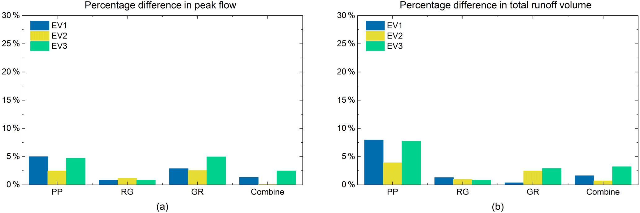
Figure 15(a) Percentage difference in peak flow between the same types of NBS scenarios under the three uniform rainfall events. (b) Percentage difference in total runoff volume between the same types of NBS scenarios under the three uniform rainfall events.
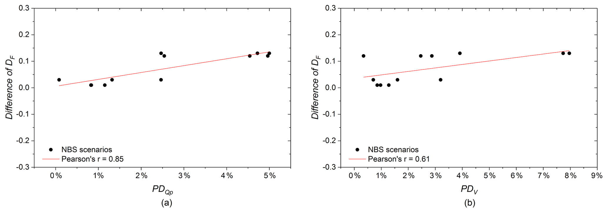
Figure 16(a) Relationship between the difference in DF of the same types of NBS scenarios and PDQp of the same types of NBS scenarios. (b) Relationship between the difference in DF of the same types of NBS scenarios and PDV of the same types of NBS scenarios.
4.4 Intersection effects of spatial variability in rainfall and spatial arrangement of NBSs
In the following, we present the results of the third modelling experiment set described in Sect. 3.3. The aim is to analyse the potential intersection effects of the spatial variability in rainfall and spatial distribution of NBSs on the hydrological responses of NBS scenarios.
The resulting uncertainty of the peak flow and total runoff volume (PD and PDV) of the third set of modelling experiments is shown in Fig. 17. First, we found that the spatial variability in rainfall has an impact to a certain extent on the peak flow of each scenario, with the PD ranging from about 8 % to 18 %. With the exception of GR1, all the NBS scenarios have a similar tendency in that the PD are the lowest for the first event and the highest for the second one. Namely, for most of NBS scenarios, the PD (uncertainty on peak flow) increases with the increase in the spatial variability in rainfall intensity. As shown in Fig. 17c, when comparing the PD between scenarios of PP1 and PP2, RG1 and RG2, as well as Combined1 and Combined2 for the three rainfall events, the maximum difference is less than 3 %. However, when comparing the PD between GR1 and GR2, the difference is larger, especially in EV3 (> 6 %). For the GR1 scenario, PD range from about 8.7 % to 18 % in all three rainfall events, and those of GR2 range from about 10.7 % to 16 %. Furthermore, for GR1, the largest PD is in EV3, but for GR2, the largest PD is computed for EV2. The difference in PD between GR1 and GR2 scenarios demonstrated that the spatial variability in rainfall and the spatial arrangement of GR measures have some intersection effects on the peak flow of GR scenarios. However, it is not evident for the other NBS scenarios. One of the reasons has been discussed in Sect. 4.2.2. In the GR1 scenario, GR measures are mainly implemented in the northern part of the catchment, which coincidently received higher rainfall (distributed EV3); namely, the hot spots of the rainfall field were highly intersected by the GR measures due to their high fractal dimension. Therefore, the peak flow was effectively reduced by the GRs. On the contrary, for the GR2 scenario, the GR measures are mainly located on the southern side of the catchment, which scarcely intersected with the rainfall spikes. Thus, when comparing with the GR1 scenario, the difference in the GR2 scenario simulated under the distributed rainfall and uniform rainfall is less significant. Another possible reason is that GR has the lowest storage capacity in the studied NBSs, and the studied rainfall events are not intense enough to saturate the other types of NBSs (see Versini et al., 2016 for a comparison of different properties of GR). Her et al. (2017) also indicated that the hydrological performances of NBSs are sensitive to their configurations. However, the most plausible reason is that the intersection effect is more perceptible for GRs, as they only respond to local precipitation, while it is often masked for other NBS measures that must also mitigate runoff received from other parts of the watershed. Indeed, the already mentioned integrative character of runoff should reduce the evidence for intersection effects in other NBS scenarios, whether for distributed or uniform rainfall. Similar to Fig. 13, Fig. 17 demonstrates the percentage difference in peak flow, which is much higher than that of the total runoff for each scenario. The reason is the same as explained in Sect. 4.2.2.
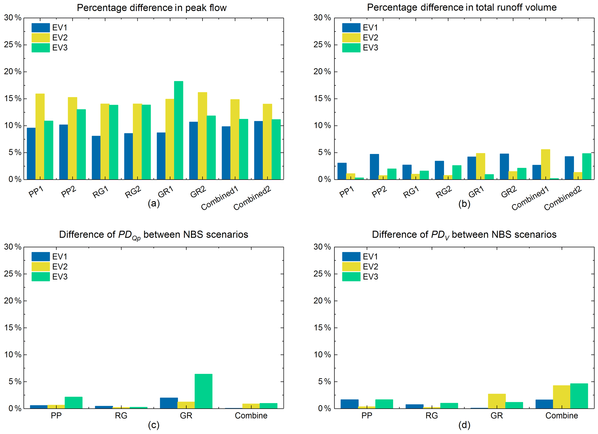
Figure 17(a) Percentage difference in peak flow of all NBS scenarios under the three distributed rainfall events and the three uniform rainfall events. (b) Percentage difference in total runoff volume of all NBS scenarios under the three distributed rainfall events and the three uniform rainfall events. (c) Difference in PDQp between the same types of NBS scenarios. (d) Difference in PDV between the same types of NBS scenarios.
Concerning the intersection impact on total runoff volume of NBS scenarios, the variations in PDV among most of NBS scenarios pairs (PP1 and PP2, GR1 and GR2, as well as Combined1 and Combined2) are significantly different for the three rainfall events. The maximum discrepancy (around 5 %) is found between Combined1 and Combined2 in EV3. Indeed, the NBSs can effectively reduce the water volume until their saturation, in particular when they largely intersect with higher rainfall. Lower intersect results in higher simulated flows and longer transfers. Furthermore, the cumulative distributed rainfall is more variable for EV3. Conversely, the difference in PDV between RG1 and RG2 is relatively small, which is less than 1 %. The reason can be explained by the large retention capacity of RG measures, which has been mentioned in Sect. 4.3.
To further investigate the intersection effects, the fourth subset of modelling experiment is used. As shown in the hydrographs (Fig. 18), the peak flow of the GR1 scenario was expected to be less than that of GR2, and this is confirmed for EV4, EV5, and EV6. For EV4 and EV5, with the same maximum intensity of 55 mm h−1, the hydrographs of these two events significantly differ, with the peak flow decreasing by a factor of 2 for EV5. However, the only difference in the rainfall inputs is that there is zero rainfall outside of the GRs during the 3 min rainfall peak. The PD and PDV of GR1 and GR2 scenario under the EV4 is around 5 % and 4.3 %, respectively (see Fig. 19). For EV5, the PD and PDV increase to 20.7 % and 7.8 %, respectively. This confirms that, without the impact of runoff that generated by other land uses, the intersection effects increase considerably with the higher spatial variability in rainfall intensity. For the EV6, the maximum rainfall intensity during the 3 min has been decreased to 17 mm h−1. This was sufficient to further reduce the peak flow during the principal rainfall peak. For this event, the PD and PDV values drop to 3.5 % and 1.8 %, respectively. This indicates that the intersection effects is less significant for the rainfall with the lower spatial variability in rainfall intensity. As expected in the EV7 scenario, because of zero rainfall intersected with the GRs in GR1 scenario, the peak flow of GR2 remains slightly lower than that of the GR1, with the PD and PDV values of only 2.1 % and 1.4 %, respectively.
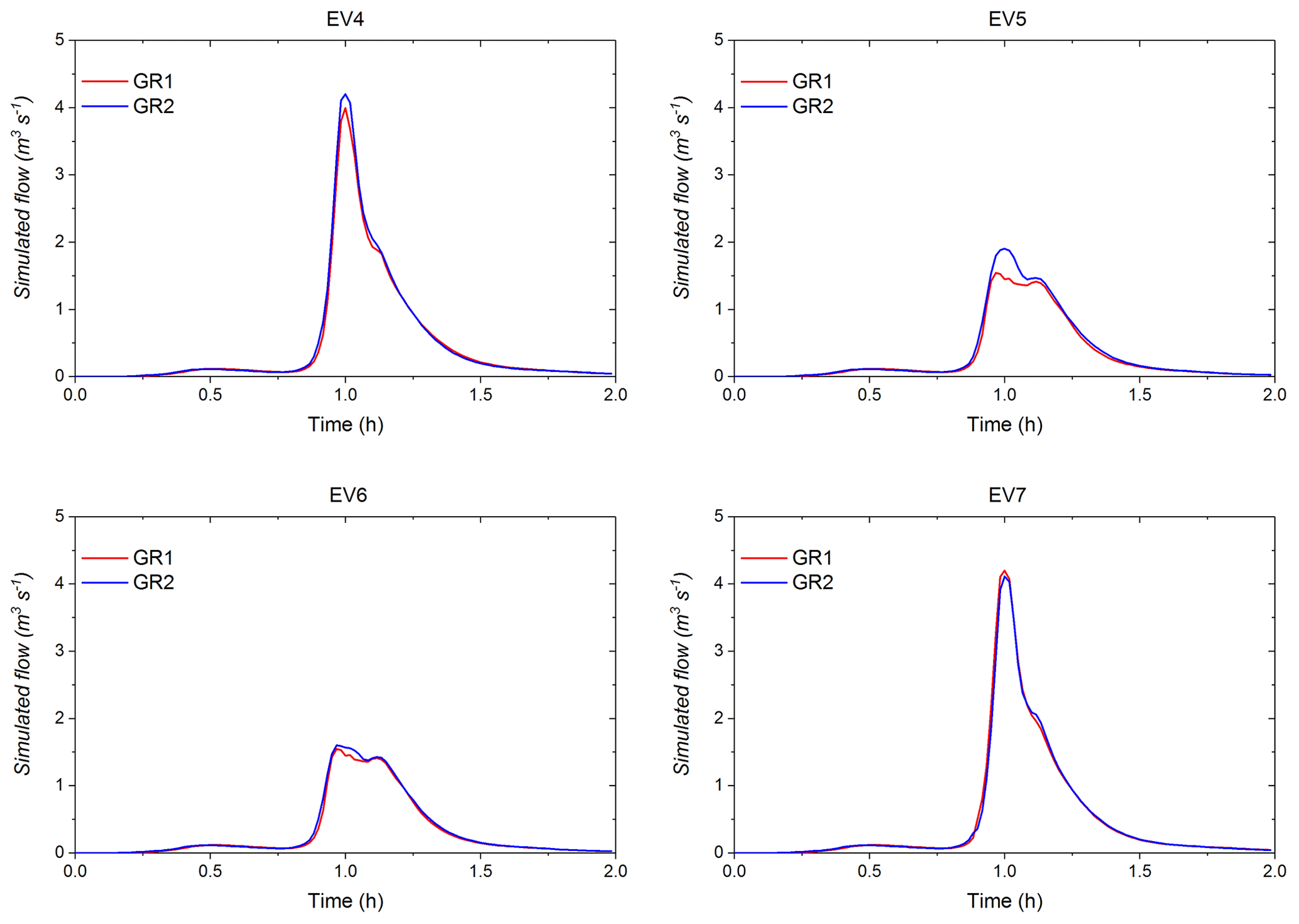
Figure 18Simulated flow (cubic metres per second) of GR1 and GR2 scenarios under the four syntactic rainfall events.
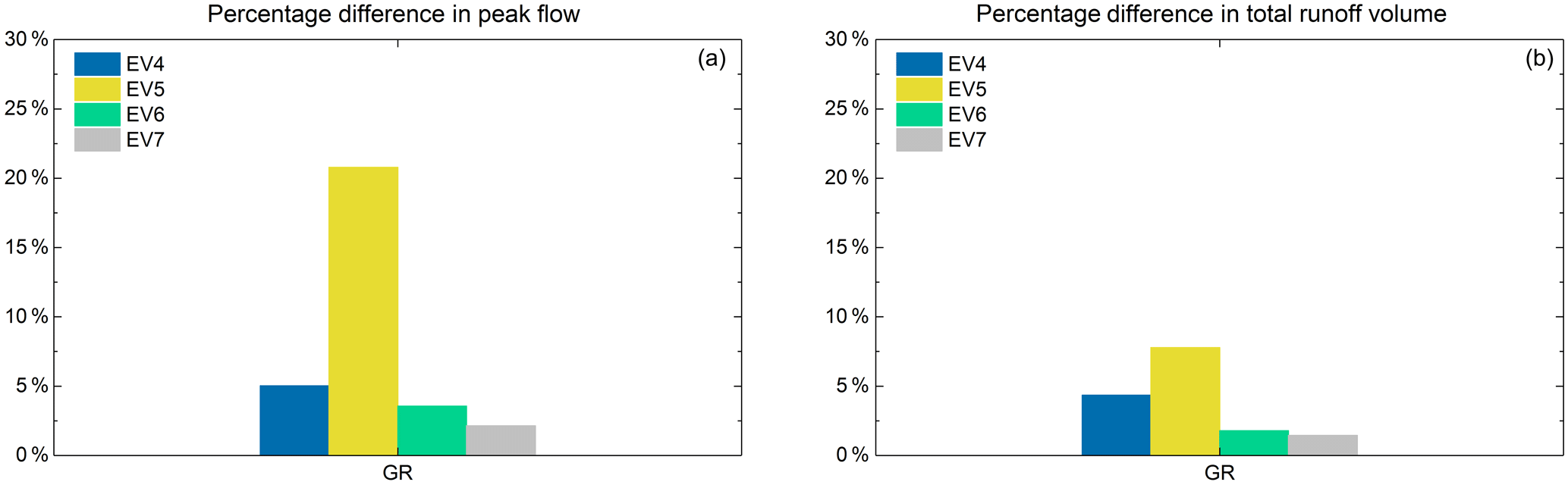
Figure 19(a) Percentage difference in peak flow of GR scenarios under the four syntactic rainfall events. (b) Percentage difference in total runoff volume of GR scenarios under the four syntactic rainfall events.
Overall, the results demonstrate that the spatial variability in rainfall and the spatial arrangement of NBSs can generate uncertainties of peak flow and total runoff volume estimations if they are not considered properly. This suggests that the performances of NBS scenarios that have been evaluated by some studies, by only applying uniform rainfall as input, can be biased in terms of the intersection effects (Zahmatkesh et al., 2015; Ahiablame and Shakya, 2016; Guo et al., 2019). In our specific case, the intersection effect is more significant for GR scenarios and combined scenarios in terms of peak flow and total runoff volume, respectively. However, the physical properties of NBSs are indeed another significant factor for the overall performances of the scenario (Gilroy et al., 2009); for example, the intersection effect is less evident for RG scenarios, mainly due to their high storage capacity. Compared to the impacts of spatial variability in rainfall on the hydrological responses of NBSs, the intersection effects seem to be less significant. These results also further demonstrated that the hydrological responses of the NBS scenario is less influenced by the spatial distributions of NBSs. As the rainfall fields are always variable in space and time, to make the most of the benefits of NBSs for storm water management, the results suggest implementing NBSs scattered in the catchment but with a higher fractal dimension DF. This will combine a lower investment with the maximum return, preventing NBSs from concentrated in certain specific places.
This paper studies the uncertainty of the hydrological responses of nature-based solution (NBS) scenarios resulting from the multiscale spatial variability in rainfall and heterogeneous distribution of NBSs at the urban catchment scale. As an application of the multifractal approach, we pointed out how the “multifractal intersection theorem” can quantify how often they intersect, which conditions the performance of NBSs. The high-resolution distributed rainfall data from the École des Ponts ParisTech (ENPC) X-band radar depict the spatially variable rainfall fields. The fully distributed and physically based hydrological model (Multi-Hydro) takes into account the heterogeneity of an urban environment down to the 10 m scale, including the spatial arrangement of NBSs and spatial distribution of rainfall. The principal findings are summarized as follows.
The spatial variability in rainfall has a significant impact on the peak flow of NBS scenarios for the three studied rainfall events. For instance, it makes the maximum percentage difference in peak flow (PD) increase up to 18 % in the GR1 scenario. Furthermore, the spatial variability in the rainfall intensity at the largest rainfall peak is almost linearly related to the PD computed for all NBS scenarios (except for GR1); the more variable the rainfall intensities are, the higher the PD are. However, the resulting percentage difference in total runoff volume (PDV) computed for all NBS scenarios shows that the spatial variability in rainfall has a much lower impact on the uncertainty related to total runoff volume, with the average PDV being of the order of 2.3 % only.
The impact of the spatial arrangement of NBSs on hydrological responses of the catchment is less obvious. For all the NBS scenarios, PD and PDV are lower than 5 % and 8 %, respectively. However, we found that the difference in fractal dimension (DF) between the same types of NBS scenarios has a fairly strong positive correlation to the related PD. Therefore, we suggest implementing NBSs by optimizing DF over the whole catchment to be the highest possible. Furthermore, mixing different NBSs in the catchment, as presented in the two combined scenarios, can also efficiently reduce the uncertainty associated with the spatial arrangement of NBSs.
The fractal dimension DF appears as a useful tool for quantifying the spatial heterogeneity of NBSs across a range of scales. The DF of each NBS scenario is associated with the urbanization level of the catchment, which confirms that the level of implementation of NBSs is reasonable enough to match the catchment conditions. The fractal dimension combined with the fully distributed model is an innovative approach that is easily transportable to other catchments.
The spatial distribution of rainfall and the spatial arrangement of NBSs have intersection effects on the hydrological responses of NBS scenarios, which are especially significant for the peak flow of green roof (GR) scenarios (with a maximum difference between the scenario of GR1 and GR2 reaching about 6 % on peak flow). The intersection effects on the total runoff volume of each NBS scenario are quite variable because the chosen NBSs present some limitations in terms of infiltration or retention capacity during a long rainfall event with high intermittency. However, the rain garden (RG) scenarios appear to be less affected by the intersection effects, with a difference lower than 3 % on peak flow and lower than 1 % on total runoff volume, mainly due to RG measures characterized by a higher retention capacity. The results of the synthetic experiment firstly confirm that there is a complex interplay between the spatio-temporal intensity of precipitation and the runoff received from other parts of the watershed. Furthermore, this experiment strengthened the intersection effects on the GR scenarios. These intersection effects can be more significant for the rainfall events with higher spatial variability.
The study of the hydrological response in various NBS scenarios resulting from the multiscale spatial variability in precipitation and the heterogeneous distribution of NBSs hints towards using fully distributed hydrological models over semi-distributed or lumped models. Indeed, the fully distributed model has been shown to be able to take into account these small-scale heterogeneities and propagate their effects to watershed scales, while parameterizing or smoothing out some critical heterogeneity, as done in non-fully distributed models, may bias its predictions.
In our specific case, the GR scenarios are more sensitive to the spatial variability in rainfall and the spatial arrangement of GR measures, while the performances of RG scenarios and combined scenarios are more stable under any condition. Apparently, these findings already give some insight to decision-makers on why they need to prioritize given NBSs within the urban planning process.
Although the rainfall events selected for this study were not extreme events, they cover a rather broad spectrum of spatio-temporal variability in rainfall, and they are very typical precipitation in the Paris region. The simulation results can serve as a reference for future urban planning in this region. For example, the results of three different impacts (i.e. the spatial variability in precipitation, the spatial distribution of NBSs, and the intersection effects) on the performance of NBS scenarios are useful for decision-makers targeting or working towards an actual project.
However, larger precipitation samples, including extreme rains, and NBS monitoring data will be helpful for obtaining better knowledge of universal solutions and providing answers on how to prioritize these NBSs. With respect to this perspective, the obtained results already demonstrated that new scale-independent indicators, like the fractal dimension applied in this study, will be essential for a more profound quantitative evaluation of the diversity of combined impacts, including for other heterogeneous catchments. Therefore, this study has an important potential impact, due to its originality with respect to the nonlinear tools used to address such practical issues and its relevance in interdisciplinary applications. This suggests pursuing the development of original tools to obtain new insights into the scaling complexity of flows in urban hydrology.
Data sets for this study are under preparation for public release by the Chair Hydrology for Resilience Cities. They can be freely obtained from contact.hmco@enpc.fr.
Version 2.1 of Multi-Hydro is registered by the (France) Program Protection Agency (IDDN FR 001 340017 000 SC 2015 0000 31235) and can be freely obtained from contact.hmco@enpc.fr.
YQ performed the modelling experiments and data analysis and wrote the paper with contributions from all co-authors. IT and DS conceived and supervised the study. YQ and PAV created and implemented various scenarios. YQ and IdSRP prepared the input data for the model. All co-authors revised the paper.
The authors declare that they have no conflict of interest.
Yangzi Qiu greatly acknowledges the financial support from the China Scholarship Council and, furthermore, highly acknowledges Abdellah Ichiba for his precious help in taking over the Multi-Hydro model. All the authors acknowledge the Chair Hydrology for Resilient Cities (endowed by Veolia), for the partial financial support, and expresses gratitude to their colleagues from Le Syndicat Intercommunal pour l'Assainissement de la Vallée de la Bièvre (SIAVB) and Veolia, and particularly Bernard Willinger, for the many stimulating discussions. The authors acknowledge the agglomeration community of Saint-Quentin-en-Yvelines, for providing the data of the Guyancourt catchment, and also express thanks to Aderson Dionísio Leite Neto, for his help with numerical pre-processing of these data as a part of his secondment at École des Ponts ParisTech.
This research has been supported by the research scholarship (grant no. [2017]3109) from the China Scholarship Council, 2017–2020.
This paper was edited by Monica Riva and reviewed by Ruben Imhoff and one anonymous referee.
Ahiablame, L. and Shakya, R.: Modeling flood reduction effects of low impact development at a watershed scale, J. Environ. Manage., 171, 81–91, https://doi.org/10.1016/j.jenvman.2016.01.036, 2016.
Ahiablame, L. M., Engel, B. A., and Chaubey, I.: Effectiveness of low impact development practices in two urbanized watersheds: Retrofitting with rain barrel/cistern and porous pavement, J. Environ. Manage., 119, 151–161, https://doi.org/10.1016/j.jenvman.2013.01.019, 2013.
Alves de Souza, B., da Silva Rocha Paz, I., Ichiba, A., Willinger, B., Gires, A., Amorim, J. C. C., de Miranda Reis, M., Tisserand, B., Tchiguirinskaia, I., and Schertzer, D.: Multi-hydro hydrological modelling of a complex peri-urban catchment with storage basins comparing C-band and X-band radar rainfall data, Hydrolog. Sci. J., 63, 1619–16352018, https://doi.org/10.1080/02626667.2018.1520390, 2018.
Burszta-Adamiak, E. and Mrowiec, M.: Modelling of Green roofs' hydrologic performance using EPA's SWMM, Water Sci. Technol., 68, 36–42, https://doi.org/10.2166/wst.2013.219, 2013.
Bloorchian, A. A., Ahiablame, L., Osouli, A., and Zhou, J.: Modeling BMP and Vegetative Cover Performance for Highway Stormwater Runoff Reduction, in: Procedia Engineering, 145, 274–280, https://doi.org/10.1016/j.proeng.2016.04.074, 2016.
Bozovic, R., Maksimovic, C., Mijic, A., Smith, K. M., Suter, I., and van Reeuwijk, M.: Blue Green Solutions: A Systems Approach to Sustainable, Resilient and Cost-Efficient Urban Development, Technical report, https://doi.org/10.13140/RG.2.2.30628.07046, 2017.
Cipolla, S. S., Maglionico, M., and Stojkov, I.: A long-term hydrological modelling of an extensive green roof by means of SWMM, Ecol. Eng., 95, 876–887, https://doi.org/10.1016/j.ecoleng.2016.07.009, 2016.
Cohen-Shacham, E., Walters, G., Janzen, C., and Maginnis, S.: Nature-based solutions to address global societal challenges, IUCN: Gland, Switzerland, 97, https://doi.org/10.2305/IUCN.CH.2016.13.en, 2016.
Chan, F., Griffiths, J., Ka, F., Chan, S., Gri, J. A., Higgitt, D., Xu, S., and Zhu, F.: “ Sponge City ” in China – A breakthrough of planning and flood risk management in the urban context, Land Use Policy, 76, 772–778, https://doi.org/10.1016/j.landusepol.2018.03.005, 2018.
Dussaillant, A. R., Wu, C. H., and Potter, K. W.: Richards Equation Model of a Rain Garden, J. Hydrol. Eng., 9, 219–225, https://doi.org/10.1061/(ASCE)1084-0699(2004)9:3(219), 2004.
El Tabach, E., Tchiguirinskaia, I., Mahmood, O., and Schertzer, D.: Multi-Hydro: a spatially distributed numerical model to assess and manage runoff processes in peri-urban watersheds. In Proceedings Final Conference of the COST Action C22 Urban Flood Management, Paris, 26 (no. 27.11), 2009, 2009.
Ercolani, G., Chiaradia, E. A., Gandolfi, C., Castelli, F., and Masseroni, D.: Evaluating performances of green roofs for stormwater runoff mitigation in a high flood risk urban catchment, J. Hydrol., 566, 830–845, https://doi.org/10.1016/j.jhydrol.2018.09.050, 2018.
European Commission: Towards an EU Research and Innovation policy agenda for Nature-Based Solutions & Re-Naturing Cities, Final Report of the Horizon 2020 Expert Group on “Nature-Based Solutions and Re-Naturing Cities”, Luxembourg: Publications Office of the European Union, https://doi.org/10.2777/765301, 2015.
Fry, T. J. and Maxwell, R. M.: Evaluation of distributed BMPs in an urban watershed – High resolution modeling for stormwater management, Hydrol. Process., 31, 2700–2712, https://doi.org/10.1002/hyp.11177, 2017.
Giangola-Murzyn, A.: Modélisation et paramétrisation hydrologique de la ville, résilience aux inondations, PhD thesis, Ecole des Ponts ParisTech, Université Paris-Est, France, 260 pp., 2013.
Giangola-Murzyn, A., Richard, J., Gires, A., Fitton, G., Tchiguirinskaia, I., and Schertzer, D.: Multi-Hydro Notice and Tutorial. Laboratoire Eau Environnement et Systèmes Urbains, École des Ponts ParisTech. Université Paris-Est, France, 44 pp., 2014.
Gires, A., Tchiguirinskaia, I., Schertzer, D., and Lovejoy, S.: Multifractal analysis of a semi-distributed urban hydrological model, Urban Water J., 10, 195–208, https://doi.org/10.1080/1573062X.2012.716447, 2013.
Gires, A., Giangola-Murzyn, A., Abbes, J. B., Tchiguirinskaia, I., Schertzer, D., and Lovejoy, S.: Impacts of small scale rainfall variability in urban areas: a case study with 1D and 1D/2D hydrological models in a multifractal framework, Urban Water J., 12, 607–617, https://doi.org/10.1080/1573062X.2014.923917, 2015.
Gires, A., Tchiguirinskaia, I., Schertzer, D., Ochoa-Rodriguez, S., Willems, P., Ichiba, A., Wang, L.-P., Pina, R., Van Assel, J., Bruni, G., Murla Tuyls, D., and ten Veldhuis, M.-C.: Fractal analysis of urban catchments and their representation in semi-distributed models: imperviousness and sewer system, Hydrol. Earth Syst. Sci., 21, 2361–2375, https://doi.org/10.5194/hess-21-2361-2017, 2017.
Gires, A., Abbes, J.-B., da Silva Rocha Paz, I., Tchiguirinskaia, I., and Schertzer, D.: Multifractal characterisation of a simulated surface flow: a case study with multi-hydro in Jouy-en-Josas, France, J. Hydrol., 558, 483–495, https://doi.org/10.1016/j.jhydrol.2018.01.062, 2018.
Gilroy, K. L. and McCuen, R. H.: Spatio-temporal effects of low impact development practices, J. Hydrol., 367, 228–236, https://doi.org/10.1016/j.jhydrol.2009.01.008, 2009.
Guo, X., Du, P., Zhao, D., and Li, M.: Modelling low impact development in watersheds using the storm water management model, Urban Water J., 16, 146–155, https://doi.org/10.1080/1573062X.2019.1637440, 2019.
Hentschel, H. G. E. and Procaccia, I.: The infinite number of generalized dimensions of fractals and strange attractors, Physica D, 8, 435–444, https://doi.org/10.1016/0167-2789(83)90235-X, 1983.
Healy, R. W.: Simulation of solute transport in variably saturated porous media with supplemental information on modifications to the US Geological Survey's computer program VS2D, U.S. Geol. Surv. Water-Resources Investig. Rep. 90-4025, https://doi.org/10.3133/wri904025, 1990.
Hoang, T.: Prise en compte des fluctuations spatio-temporelles pluies-débits pour une meilleure gestion de la ressource en eau et une meilleure évaluation des risques, PhD Thesis, Earth Sciences, Université Paris-Est, Champs-sur-Marne, France, 2011.
Holman-Dodds, J. K., Bradley, A. A., and Potter, K. W.: Evaluation of hydrologic benefits of infiltration based urban storm water management, J. Am. Water Resour. Assoc., 39, 205–215, https://doi.org/10.1111/j.1752-1688.2003.tb01572.x, 2003.
Her, Y., Jeong, J., Arnold, J., Gosselink, L., Glick, R., and Jaber, F.: A new framework for modeling decentralized low impact developments using Soil and Water Assessment Tool, Environ. Model. Softw., 96, 305–322, https://doi.org/10.1016/j.envsoft.2017.06.005, 2017.
Hu, M., Sayama, T., Zhang, X., Tanaka, K., Takara, K., and Yang, H.: Evaluation of low impact development approach for mitigating flood inundation at a watershed scale in China, J. Environ. Manage., 193, 430–438, https://doi.org/10.1016/j.jenvman.2017.02.020, 2017.
Hamidi, A., Farnham, D. J., and Khanbilvardi, R.: Uncertainty analysis of urban sewer system using spatial simulation of radar rainfall fields: New York City case study, Stoch. Environ. Res. Risk Assess., 32, 2293–2308, https://doi.org/10.1007/s00477-018-1563-8, 2018.
Ichiba, A.: X-Band Radar Data and Predictive Management in Urban Hydrology, PhD Thesis, Earth Sciences, Université Paris-Est, Champs-sur-Marne, France, 2016.
Ichiba, A., Gires, A., Tchiguirinskaia, I., Schertzer, D., Bompard, P., and Ten Veldhuis, M.-C.: Scale effect challenges in urban hydrology highlighted with a distributed hydrological model, Hydrol. Earth Syst. Sci., 22, 331–350, https://doi.org/10.5194/hess-22-331-2018, 2018.
Imhoff, R. O., Van Verseveld, W. J., Van Osnabrugge, B., and Weerts, A. H.: Scaling Point-Scale (Pedo) transfer Functions to Seamless Large-Domain Parameter Estimates for High-Resolution Distributed Hydrologic Modeling: An Example for the Rhine River, Water Resour. Res., 56, 1–28, https://doi.org/10.1029/2019WR026807, 2020.
Institut National de la Statistique et des Etudes Economiques – INSEE: Dossier complet – Commune de Guyancourt (78297), available at: https://www.insee.fr/fr/statistiques/2011101?geo=COM-78297#chiffre-cle-5, last access: 29 February 2020.
James, W., Rossman, L. A., and James, W. R. C.: User's guide to SWMM5 based on original USEPA SWMM documentation, CHI, USA, 905, 2010.
Jia, H., Yao, H., Tang, Y., Yu, S. L., Field, R., and Tafuri, A. N.: LID-BMPs planning for urban runoff control and the case study in China, J. Environ. Manage., 149, 65–76, https://doi.org/10.1016/j.jenvman.2014.10.003, 2015.
Kelman, I.: Climate Change and the Sendai Framework for Disaster Risk Reduction, Int. J. Disaster Risk Sc., 6, 117–127, https://doi.org/10.1007/s13753-015-0046-5, 2015.
Kuang, X., Sansalone, J., Ying, G., and Ranieri, V.: Pore-structure models of hydraulic conductivity for permeable pavement, J. Hydrol., 399, 148–157, https://doi.org/10.1016/j.jhydrol.2010.11.024, 2011.
Kwak, D., Kim, H., and Han, M.: Runoff Control Potential for Design Types of Low Impact Development in Small Developing Area Using XPSWMM, Procedia Engineering., 154, 1324–1332, https://doi.org/10.1016/j.proeng.2016.07.483, 2016.
Lappala, E. G., Healy, R. W., and Weeks, E. P.: Documentation of computer program VS2D to solve the equations of fluid flow in variably saturated porous media, Department of the Interior, US Geological Survey, 83-4099, https://doi.org/10.3133/wri834099, 1987.
Lavallée, D., Lovejoy, S., Schertzer, D., and Ladoy, P.: Nonlinear variability and landscape topography: analysis and simulation, Fractals in Geography, 158–192, 1993.
Liu, Y., Ahiablame, L. M., Bralts, V. F., and Engel, B. A.: Enhancing a rainfall-runoff model to assess the impacts of BMPs and LID practices on storm runoff, J. Environ. Manage., 147, 12–23, https://doi.org/10.1016/j.jenvman.2014.09.005, 2015.
Loukas, A., Llasat, M.-C., and Ulbrich, U.: Preface “Extreme events induced by weather and climate change: evaluation, forecasting and proactive planning”, Nat. Hazards Earth Syst. Sci., 10, 1895–1897, https://doi.org/10.5194/nhess-10-1895-2010, 2010.
Lovejoy, S. and Schertzer, D.: The weather and climate: Emergent laws and multifractal cascades, Cambridge University Press, UK, 491, 2013.
Lovejoy, S., Schertzer, D., and Tsonis, A. A.: Functional Box-Counting and Multiple Elliptical Dimensions in Rain, Science, 235, 1036–1038, https://doi.org/10.1126/science.235.4792.1036, 1987.
Lucas, W. C. and Sample, D. J.: Reducing combined sewer overflows by using outlet controls for Green Stormwater Infrastructure: Case study in Richmond, Virginia, J. Hydrol., 520, 473–488, https://doi.org/10.1016/j.jhydrol.2014.10.029, 2015.
Mandelbrot, B. B.: The fractal geometry of nature, W.H. Freeman and Company, New York, 468, 1983.
Massoudieh, A., Maghrebi, M., Kamrani, B., Nietch, C., Tryby, M., Aflaki, S., and Panguluri, S.: A flexible modeling framework for hydraulic and water quality performance assessment of stormwater green infrastructure, Environ. Model. Softw., 92, 57–73, https://doi.org/10.1016/j.envsoft.2017.02.013, 2017.
Météo-France: Climat des Yvelines, available at: https://www.meteofrance.com/accueil, last access: 29 February 2020.
Miller, J. D. and Hutchins, M.: The impacts of urbanisation and climate change on urban flooding and urban water quality: A review of the evidence concerning the United Kingdom, J. Hydrol., 12, 345–362, https://doi.org/10.1016/j.ejrh.2017.06.006, 2017.
Mooers, E. W., Eng, P., Jamieson, R. C., Eng, P., Hayward, J. L., Eng, P., Drage, J., Lake, C. B., and Eng, P.: Low-Impact Development Effects on Aquifer Recharge Using Coupled Surface and Groundwater Models, J. Hydrol. Eng., 23, 1–11, https://doi.org/10.1061/(ASCE)HE.1943-5584.0001682, 2018.
Morison, P. J. and Brown, R. R.: Landscape and Urban Planning Understanding the nature of publics and local policy commitment to Water Sensitive Urban Design, Landscape Urban Plan., 99, 83–92, https://doi.org/10.1016/j.landurbplan.2010.08.019, 2011.
Nash, J. E., and Sutcliffe, J. V.: River flow forecasting through conceptual models part I – A discussion of principles, J. Hydrol., 10, 282–290, https://doi.org/10.1016/0022-1694(70)90255-6, 1970.
Newcomer, M. E., Gurdak, J. J., Sklar, L. S., and Nanus, L.: Urban recharge beneath low impact development and effects of climate variability and change, Water Resour. Res., 50, 1716–1734, https://doi.org/10.1002/2013WR014282, 2014.
Ochoa-rodriguez, S., Wang, L., Gires, A., Daniel, R., Reinoso-rondinel, R., Bruni, G., Ichiba, A., Gaitan, S., Cristiano, E., Assel, J. Van, Kroll, S., Murlà-tuyls, D., Tisserand, B., Schertzer, D., Tchiguirinskaia, I., Onof, C., Willems, P., and Veldhuis, M.: Impact of spatial and temporal resolution of rainfall inputs on urban hydrodynamic modelling outputs: A multi-catchment investigation, J. Hydrol., 531, 389–407, https://doi.org/10.1016/j.jhydrol.2015.05.035, 2015.
Park, D., Sandoval, N., Lin, W., Kim, H., and Cho, Y.: A case study: Evaluation of water storage capacity in permeable block pavement, J. Civ. Eng., 18, 514–520, https://doi.org/10.1007/s12205-014-0036-y, 2014.
Palla, A., Gnecco, I., Carbone, M., Garofalo, G., Lanza, L. G., and Piro, P.: Influence of stratigraphy and slope on the drainage capacity of permeable pavements: laboratory results, Urban Water J., 12, 394–403, https://doi.org/10.1080/1573062X.2014.900091, 2015.
Paz, I., Willinger, B., Gires, A., Ichiba, A., Monier, L., Zobrist, C., Tisserand, B., Tchiguirinskaia, I., and Schertzer, D.: Multifractal comparison of reflectivity and polarimetric rainfall data from C- and X-band radars and respective hydrological responses of a complex catchment model, Water, 10, 269, https://doi.org/10.3390/w10030269, 2018.
Paz, I., Willinger, B., Gires, A., Alves de Souza, B., Monier, L., Cardinal, H., Tisserand, B., Tchiguirinskaia, I., and Schertzer, D.: Small-Scale Rainfall Variability Impacts Analyzed by Fully-Distributed Model Using C-Band and X-Band Radar Data, Water, 11, 1273, https://doi.org/10.3390/w11061273, 2019.
Paz, I., Tchiguirinskaia, I., and Schertzer, D.: Rain gauge networks' limitations and the implications to hydrological modelling highlighted with a X-band radar, J. Hydrol., 583, 124615, https://doi.org/10.1016/j.jhydrol.2020.124615, 2020.
Qin, H. P., Li, Z. X., and Fu, G.: The effects of low impact development on urban flooding under different rainfall characteristics, J. Environ. Manage., 129, 577–585, https://doi.org/10.1016/j.jenvman.2013.08.026, 2013.
Richard, J., Giangola-Murzyn, A., Tchiguirinskaia, I., and Schertzer, D.: MH-ASSIMTOOL: An assimilation tool dedicated to a fully distributed model. Poster presented at International Conference on Flood Resilience, 5–7 September 2013, United Kingdom, 2013.
Riva, M., Guadagnini, L., Guadagnini, A., Ptak, T., and Martac, E.: Probabilistic study of well capture zones distribution at the Lauswiesen field site, J. Contam. Hydrol., 88, 92–118, https://doi.org/10.1016/j.jconhyd.2006.06.005, 2006.
Rossman, L. A.: Storm water management model user's manual, version 5.0, Cincinnati: National Risk Management Research Laboratory, Office of Research and Development, US Environmental Protection Agency, 276, 2010.
Scherzter, D. and Lovejoy, S.: On the dimension of atmospheric motions, Turbulence and Chaotic phenomena in Fluids, edited by: Tatsumi, T., Elsevier North-Holland, 505–512, 1984.
Schertzer, D. and Lovejoy, S.: Physical modeling and analysis of rain and clouds by anisotropic scaling multiplicative processes, J. Geophys. Res.-Atmos., 92, 9693–9714, https://doi.org/10.1029/JD092iD08p09693 1987.
Schertzer, D. and Lovejoy, S.: Nonlinear variability in geophysics, Kluwer Academic Publishers, the Netherlands, 303, https://doi.org/10.1007/978-94-009-2147-4, 1991.
Schertzer, D., Tchiguirinskaia, I., Lovejoy, S., and Hubert, P.: No monsters, no miracles: in nonlinear sciences hydrology is not an outlier!, Hydrolog. Sci. J., 55, 965–979, https://doi.org/10.1080/02626667.2010.505173, 2010.
Sun, Y. W., Li, Q. Y., Liu, L., Xu, C. D., and Liu, Z. P.: Hydrological simulation approaches for BMPs and LID practices in highly urbanized area and development of hydrological performance indicator system, Water Sci. Eng., 7, 143–154, https://doi.org/10.3882/j.issn.1674-2370.2014.02.003, 2014.
Stanić, F., Cui, Y. J., Delage, P., De Laure, E., Versini, P. A., Schertzer, D., and Tchiguirinskaia, I.: A device for the simultaneous determination of the water retention properties and the hydraulic conductivity function of an unsaturated coarse material; application to a green-roof volcanic substrate, Geotech. Test. J., 43, https://doi.org/10.1520/GTJ20170443, 2019.
Tchiguirinskaia, I., Schertzer, D., Hubert, P., Bendjoudi, H., and Lovejoy, S.: Multiscaling geophysics and sustainable development, IAHS Publ. Proc. Reports, 287, 113–136, 2004.
Velleux, M. L., England, J. F., and Julien, P. Y.: TREX: spatially distributed model to assess watershed contaminant transport and fate, Sci. Total Environ., 404, 113–128, https://doi.org/10.1016/j.scitotenv.2008.05.053, 2008.
Versini, P. A., Gires, A., Tchinguirinskaia, I., and Schertzer, D.: Toward an operational tool to simulate green roof hydrological impact at the basin scale: A new version of the distributed rainfall-runoff model Multi-Hydro, Water Sci. Technol., 74, 1845–1854, https://doi.org/10.2166/wst.2016.310, 2016.
Versini, P. A., Kotelnikova, N., Poulhes, A., Tchiguirinskaia, I., Schertzer, D., and Leurent, F.: A distributed modelling approach to assess the use of Blue and Green Infrastructures to fulfil stormwater management requirements, Landscape Urban Plan., 173, 60–63, https://doi.org/10.1016/j.landurbplan.2018.02.001, 2018.
Versini, P.-A., Gires, A., Tchiguirinskaia, I., and Schertzer, D.: Fractal analysis of green roof spatial implementation in European cities, Urban For. Urban Gree., 49, 126629, https://doi.org/10.1016/j.ufug.2020.126629, 2020.
Zahmatkesh, Z., Burian, S. J., Karamouz, M., Tavakol-Davani, H., and Goharian, E.: Low-Impact Development Practices to Mitigate Climate Change Effects on Urban Stormwater Runoff: Case Study of New York City, J. Irrig. Drain. Eng., 141, 4014043, https://doi.org/10.1061/(ASCE)IR.1943-4774.0000770, 2015.
Zhu, Z., Chen, Z., Chen, X., and Yu, G.: An assessment of the hydrologic effectiveness of low impact development (LID) practices for managing runoff with different objectives, J. Environ. Manage., 231, 504–514, https://doi.org/10.1016/j.jenvman.2018.10.046, 2019.