Assessing interannual variability in nitrogen sourcing and retention through hybrid Bayesian watershed modeling

Excessive nutrient loading is a major cause of water quality problems worldwide, often leading to harmful algal blooms and hypoxia in lakes and coastal systems. Efficient nutrient management requires that loading sources are accurately quantified. However, loading rates from various urban and rural non-point sources remain highly uncertain especially with respect to climatological variation. Furthermore, loading models calibrated using statistical techniques (i.e., hybrid models) often have limited capacity to differentiate export rates among various source types, given the noisiness and paucity of observational data common to many locations. To address these issues, we leverage data for two North Carolina Piedmont river basins collected over three decades (1982–2017) using a mechanistically parsimonious watershed loading and transport model calibrated within a Bayesian hierarchical framework. We explore temporal drivers of loading by incorporating annual changes in precipitation, land use, livestock, and point sources within the model formulation. Also, different representations of urban development are compared based on how they constrain model uncertainties. Results show that urban lands built before 1980 are the largest source of nutrients, exporting over twice as much nitrogen per hectare than agricultural and post-1980 urban lands. In addition, pre-1980 urban lands are the most hydrologically constant source of nutrients, while agricultural lands show the most variation among high- and low-flow years. Finally, undeveloped lands export an order of magnitude (∼7–13×) less nitrogen than built environments.

1 Introduction

Eutrophication stimulated by anthropogenic nutrient loading is a common cause of water quality problems worldwide (Smith et al., 1999). In North Carolina (NC, USA), watershed-level nutrient management strategies have been developed for major reservoirs like Jordan Lake (JL) and Falls Lake (FL) using various process-based models (NC DWR, 2009; Tetra Tech, 2014). Such models can operate on fine temporal scales (i.e., days) and characterize various mechanistic processes related to the transfer of water and nutrients through watersheds. However, due to the large number of uncertain parameters (i.e., rates, coefficients) included in these models, multiple parameter sets may appear to fit the observational data equally well (Beven, 2006) without benefits to predictive performance (Jackson-Blake et al., 2017). Related to these issues, there is critical need for systematic model calibration and uncertainty quantification, if modeling results are to inform management decisions (Reckhow, 1994; NRC, 2001; Reichert, 2020).

Hybrid (empirical–mechanistic) watershed models, which represent nutrient loading, transport, and retention using simple mechanistic relationships and statistical calibration techniques (e.g., nonlinear regression, Bayesian inference), have also been developed for nutrient source apportionment. For example, numerous applications of the SPAtially Referenced Regressions of contaminant transport On Watershed attributes (SPARROW) model have been applied to many large river basins (Preston et al., 2011; Hoos and McMahon, 2009; Garcia et al., 2011). SPARROW is calibrated using nonlinear regression that allows for parameter uncertainty quantification (i.e., confidence intervals). A limitation of SPARROW is that it models long-term average conditions and does not directly consider variability due to changes in precipitation (e.g., wet versus dry years) and watershed development, which have been shown to greatly affect nutrient loading (Howarth et al., 2012; Sinha and Michalak, 2016; Strickling and Obenour, 2018).

Methodological enhancements to SPARROW and similar hybrid watershed models have been proposed over time (Qian et al., 2005; Wellen et al., 2012; Xia et al., 2016). Recently, a Bayesian–hierarchical hybrid watershed model was developed to leverage temporal variability in source distributions and precipitation over multiple decades, providing an assessment of how land use change and hydroclimatological variations have affected nutrient loading over time (Strickling and Obenour, 2018). Additionally, this approach systematically incorporated and updated prior information on nutrient export and retention rates from previous studies through Bayesian inference. At the same time, Bayesian hybrid models often show limited capacity to differentiate loading rates among multiple source types (e.g., different land uses). Previous applications typically included only a small number of source types or had wide posterior credible intervals for export rates (e.g., Qian et al., 2005; Wellen et al., 2012; Strickling and Obenour, 2018).

The goal of this study is to improve our understanding of nitrogen export within two highly managed NC basins that feed critical water supply reservoirs. Using a Bayesian hybrid watershed modeling approach, we characterize export rates from several different land uses, livestock types, and point sources. In particular, we explore how nitrogen-loading estimates vary among different types of urban lands based on density and the age of construction, considering how improved regulations and building practices may influence nutrient export. In addition, we demonstrate a novel approach for characterizing interannual variability in both nitrogen export and stream and water-body retention, based on mean annual precipitation. This study benefits from a relatively high-resolution monitoring network (with a mean watershed monitoring unit of just 321 km², compared to 1535 km² in Strickling and Obenour, 2018) and over 30 years of loading data (1982–2017). Finally, we characterize instream retention rates and partition reservoir loading into various upstream sources based on varying hydro-climatological conditions to help inform watershed management.

2 Methods

2.1 Study area

JL and FL, located in the Piedmont region of NC (Fig. 1), were impounded by the US Army Corps of Engineers in the early 1980s. Portions of each reservoir have exceeded NC water quality criteria, particularly for algae (chlorophyll a; NC DWR, 2020). JL watershed planning has been ongoing since the early 2000s, and initial total nitrogen (TN) reductions were set at 35 % for the New Hope (NH) Creek basin and 8 % for the Haw River (HR) basin. FL watershed planning was formalized in 2011, and Phase I goals of the Falls Lake Rules included a TN reduction of 40 % from major sources in the watershed (http://portal.ncdenr.org/web/fallslake/, last access: 12 March 2021). JL and FL fall within the Cape Fear River basin and Neuse River basin, respectively, but both share similar underlying hydroclimatic and soil conditions and comparable levels of anthropogenic development (Markewich et al., 1990; Strickling and Obenour, 2018).

Figure 1 The load monitoring sites (LMSs) in Jordan and Falls Lake watersheds shown with their incremental watersheds. Also shown are the 79 subwatersheds along with point sources (major and minor wastewater treatment plants – WWTP). Major basins are delineated by thick black lines.

2.2 Load monitoring sites (LMSs)

Nutrient load monitoring sites (LMSs) were identified based on locations that had sufficient flow and nutrient sampling data to calculate yearly TN loads. To be included, a site needed a minimum of 5 years of daily flow records and at least 50 water quality samples during that period of record. While somewhat context specific, these minimum conditions are generally consistent with previous studies using USGS WRTDS for load estimation (Chanat et al., 2012; Hirsch and De Cicco, 2015). All flow data were obtained from the United States Geological Survey (USGS), whereas nutrient data were obtained from the Water Quality Portal (WQP; Read et al., 2017) as well as local city managers (e.g., city of Durham). The two largest sources of nutrient data (from the WQP) came from the USGS and the NC Department of Environmental Quality (NCDEQ). Sites from these different entities were often located in close proximity. Data from water quality sites with less than 5 % deviations in watershed area and no intervening point sources were compiled together (Table 1).

Table 1 Load monitoring stations (LMSs) located in the Jordan (JL) and Falls Lake (FL) basins along with their complete drainage areas. LMSs belong to either New Hope Creek (NH) or Haw River basins of JL or FL. Years of record correspond to time that loadings could be estimated (i.e., when daily flow and monthly water quality sampling was performed). The number of total nitrogen (TN) samples available is also shown.

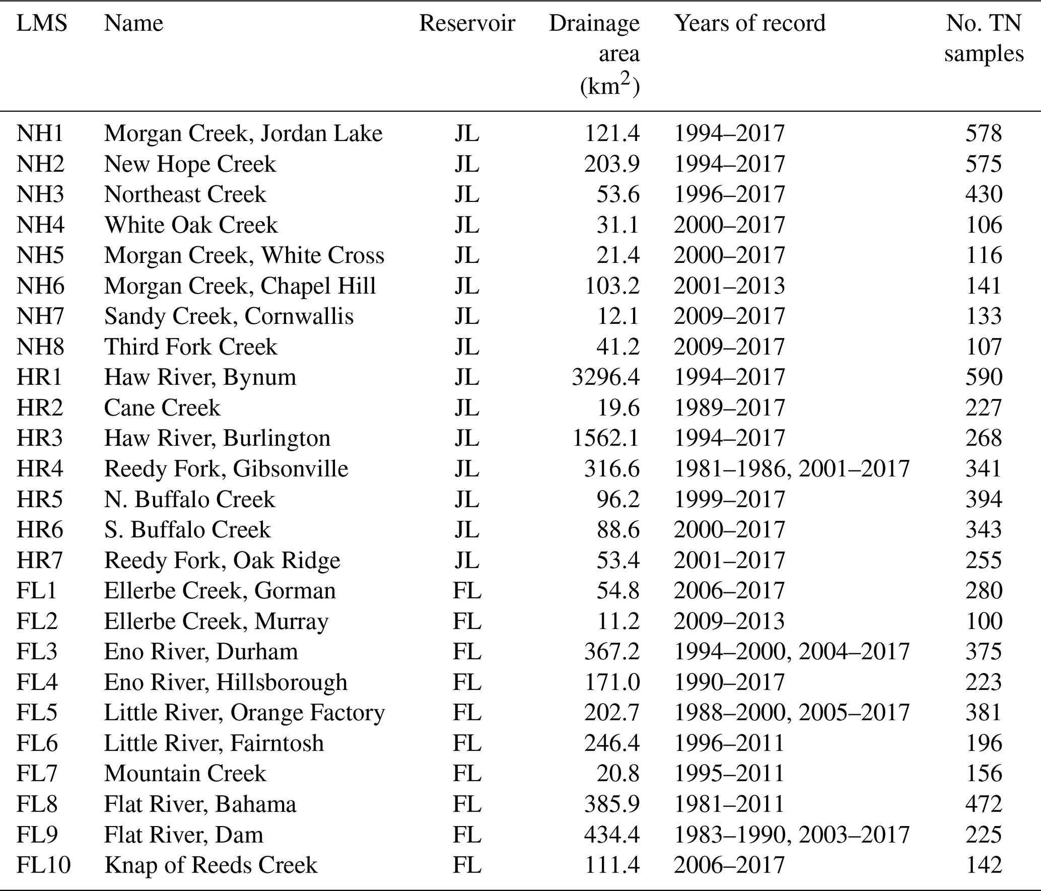
In many cases, ample water quality data were available at the location of the USGS flow monitoring station. However, if little or no water quality data were located at the flow station, a nearby water quality station was used instead, assuming there was less than a 20 % change in watershed area between the flow and water quality monitoring stations. If multiple water quality sites were located close to the flow station, only the site with the longest record was chosen. In one exception, two water quality sites utilized the same flow monitoring station (NH1 and NH6; Table 1), which was done to include two substantial data records collected above and below a major point source on Morgan Creek. In such cases, the LMSs were represented at the location of the water quality monitoring sites, and flows were adjusted based on the drainage area ratio between the two sites adjusting for any intervening wastewater flow.

There were 25 LMSs in our study area (Fig. 1; Table 1). Stations were split into three major basins for classification purposes: the HR basin of JL, the NH Creek basin of JL, and the FL basin. LMSs captured 85 % of the HR basin, 49 % of the NH basin, and 62 % of the FL basin. Three LMSs were located directly downstream of major impoundments (HR4, FL6, and FL9; Fig. 1; Table 1).

2.3 Delineation of incremental watersheds and subwatersheds

Watersheds for LMSs were delineated using Spatial Analyst tools in ArcMap 10.6.1 (ESRI, 2018). Watershed drainage areas ranged from 11 km² to over 3000 km² (Table 1) with a median value of 106 km². Often, LMS watersheds had one or more LMS contained within their upstream watershed (Fig. 1). In order to accommodate nested LMS watersheds, we determined incremental watersheds by subtracting out any upstream LMS watersheds that were contained in a larger (downstream) LMS watershed (Schwarz et al., 2006). If a LMS did not have any upstream LMSs in its watershed, its incremental watershed was equal to its total watershed. Note that the loads associated with these incremental watersheds formed the main response variable in our model (Sect. 2.7).

To more accurately account for nitrogen transport and retention, incremental watersheds were divided into subwatersheds (Fig. 1). Most data (e.g., land use, precipitation, livestock) were compiled at the subwatershed level. The largest possible subwatershed corresponded to a USGS 12-digit hydraulic unit code (HUC; https://water.usgs.gov/GIS/huc.html, last access: 15 April 2020). If a LMS was located in the middle of a HUC, the HUC was split into two. Seventy-nine subwatersheds were located within the study area, with a mean drainage area of 63 km², minimum of 11 km², and maximum of 146 km².

2.4 Anthropogenic factors

2.4.1 Land uses

Land use variables were derived from the US conterminous Wall-to-wall Anthropogenic Land use Trends (NWALT) dataset (Falcone, 2015). We aggregated NWALT land use designations into three major categories: urban (including residential, transportation, industrial, and commercial development), agriculture (pasture and crop), and undeveloped (semi-developed, low use, and wetlands). Semi-developed land was included with undeveloped because it is mostly comprised of forested land in central NC (Miller et al., 2019). We further split urbanization constructed before and after a given date (e.g., 1980, 2000) and between low and high density. To determine when urbanization occurred in the region, we interpolated available NWALT data (1974, 1982, 1992, 2002, and 2012) to obtain year-specific land use values for each subwatershed. Since our study extended beyond 2012, we also used linear extrapolation for years 2013–2017 based on 2002 and 2012 values. Land use trends throughout the study period were generally gradual, such that modest linear extrapolation was considered reasonable (Fig. 2; top row).

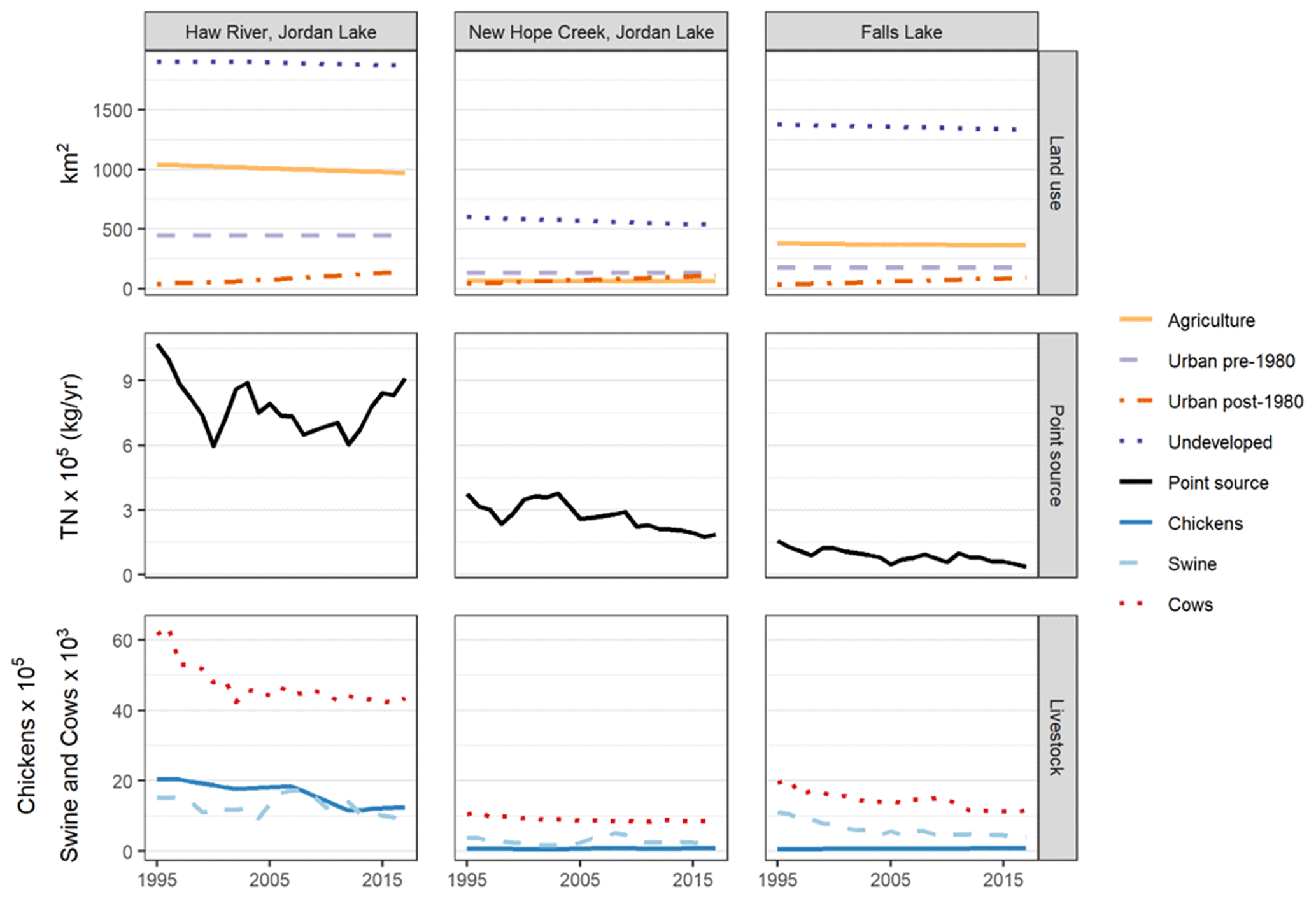
Figure 2 Land use, point sources, and livestock trends from 1994–2017 in the Haw River, New Hope, and Falls Lake basins.

2.4.2 Point sources

Point sources included major (>0.044 m³ s⁻¹) and minor wastewater treatment plants (WWTPs) (Figs. 1 and S1 in the Supplement, Table S1 in the Supplement). Discharge data were obtained from NC DEQ and included monthly TN and flow values. However, many WWTPs had numerous missing months, so we determined annual loads as the product of yearly median concentrations and flows for each WWTP. LMSs with major WWTPs in their watersheds were only modeled starting in 1994 due to a lack of discharge data before that year (i.e., HR1, 3, 5, NH1–3, and FL1, 3, 10), while LMSs without major WWTPs were modeled from 1982 depending on data availability. Only one LMS (HR4) with pre-1994 monitoring data included a minor WWTP in its watershed. Since the minor WWTP represented <3 % of the LMS mean load, we assumed the pre-1994 load was equal to the mean post-1994 load. TN trends of point source discharges aggregated by basin are shown in Fig. 2 (middle row).

2.4.3 Livestock

The livestock in subwatersheds were estimated from county-level US Department of Agriculture (USDA) census and survey reports (https://www.nass.usda.gov/, last access: 15 April 2020). Cow and swine data covered our entire study period (1982–2017), while chicken data were available every 5 years beginning in 1997. For missing years between census dates, chicken counts were interpolated, whereas chicken counts before 1997 were assumed to be equal to 1997 values. Only two incremental watersheds (HR1, 3) had large chicken counts (>1 000 000 and >150 000, respectively), and these watersheds were not modeled before 1994 (as they were also missing major WWTP discharge data).

To represent the locations of livestock throughout the region, county-level data were assigned to incremental watersheds based on an area ratio. Major urban areas were excluded when calculating these proportions, as livestock were assumed to be located outside cities. Livestock counts were then divided into the subwatersheds (using area ratios). However, chickens in Chatham County were accounted for differently because a majority of Chatham's chicken farms (>90 %) are located outside of the JL basin, and the county has a relatively high chicken count (>3 000 000; USDA). Chatham County records (https://opendata-chathamncgis.opendata.arcgis.com/, last access: 15 April 2020) were used to estimate that 8.2 % of the county's chickens were within the JL basin. Basin level trends of livestock are shown in Fig. 2 (bottom row).

2.5 Precipitation

Monthly precipitation estimates for this study were obtained from the PRISM Climate Group (http://www.prism.oregonstate.edu/, last access: 15 May 2019). These data were processed using the R package “raster” (Hijmans, 2015; R Core Team, 2019) to determine mean annual precipitation for each subwatershed. There was substantial variation in precipitation among years (0.82–1.59 m yr⁻¹) and among different subwatersheds within the same year (Fig. S2).

2.6 Nutrient load calculations

Our model required yearly TN loadings at each LMS for Bayesian inference (i.e., calibration). Most riverine monitoring programs measure streamflow daily, whereas nutrient concentrations are sampled less frequently (e.g., monthly). In this study, daily TN concentrations were estimated using WRTDS (Hirsch et al., 2010). WRTDS develops a semi-parametric regression for each day in the estimation period where observations that are collected under similar conditions to the estimation date (in terms of time, discharge, and season) are more heavily weighted. For some LMS sites, there were abrupt temporal changes in nutrient loading associated with WWTP upgrades. In these cases, WRTDS was run separately before and after the upgrade date to avoid smoothing out these transitions (Table S2).

Some LMSs had incomplete monitoring data (daily flow or water quality samples) during our study period (Table 1). If a LMS was missing flow data for a given year, that year was omitted. However, WRTDS is able to calculate loads for years with missing water quality data. Gaps in water quality samples of up to 1 year were considered acceptable in our study, as preliminary analysis (removing single years of observational data at random) showed that a 1-year gap affected loading estimates by less than 1 %, and this is more conservative than WRTDS guidelines (Hirsch and De Cicco, 2015). In addition, at least six samples were required in both the beginning and ending year of each loading record.

Uncertainties in loading estimates were determined through subsampling of three NC stations that had nearly daily TN observations for at least 7 consecutive years (Strickling and Obenour, 2018). By comparing TN loads based on the full dataset and different subsets, we estimated the coefficient of variation (and standard deviation, SD) of WRTDS estimates based on the number of water quality samples available for a given year (Fig. S3). Accounting for these uncertainties allowed us to give more weight to loading estimates based on a larger number of nutrient samples (Sect. 2.7).

The response variable in our model was the change in nutrient load across an incremental watershed, defined as the difference between the load at an incremental watershed's downstream LMS and the cumulative load from any upstream LMSs. For sites with no upstream LMSs, the incremental load was equal to its total load. The uncertainties of incremental loads for LMSs with upstream LMSs were calculated based on the relationship between correlated random variables (Eq. 1; Kottegoda and Rosso, 2008):

$$\begin{array}{}\text{(1)}& {\stackrel{\mathrm{̃}}{\mathit{\sigma }}}_{i,t}^{\mathrm{2}}={\mathit{\sigma }}_{i,t}^{\mathrm{2}}-\mathrm{2}\sum _{k=\mathrm{1}}^n{\mathit{\rho }}_{i,k}{\mathit{\sigma }}_{i,t}{\mathit{\sigma }}_{k,t}+\sum _{k=\mathrm{1}}^n\sum _{l=\mathrm{1}}^n{\mathit{\rho }}_{k,l}{\mathit{\sigma }}_{k,t}{\mathit{\sigma }}_{l,t},\end{array}$$

where ${\stackrel{\mathrm{̃}}{\mathit{\sigma }}}_{i,t}^{\mathrm{2}}$ is the incremental load variance for a given incremental watershed (i) in year (t), with n upstream LMSs (max n=3 for HR3; Fig. 1; Table 1). Here, ${\mathit{\sigma }}_{i,t}^{\mathrm{2}}$ is the error variance at the downstream LMS, σ_k,t and σ_l,t are the WRTDS SDs at upstream LMSs, and ρ_i,k and ρ_k,l are correlation coefficients between LMS loadings from different sites.

2.7 Model construction

Our model is formulated similar to Strickling and Obenour (2018). Within a Bayesian framework, we relate deterministically predicted incremental loads (${\widehat{y}}_{i,t}$; Eq. 2) to an inferred incremental load (y_i,t). The watershed-level random effect (α_i; Gelman et al., 2014) accounts for spatial variability not explained by the deterministic prediction (${\widehat{y}}_{i,t}$), and the residual error (with SD σ_ε) primarily accounts for temporal variability unexplained by the deterministic prediction. The hyperdistribution of the normally distributed watershed-level random effect is centered on zero, with variance ${\mathit{\sigma }}_{\mathrm{LMS}}^{\mathrm{2}}$.

$$\begin{array}{}\text{(2)}& \begin{array}{rl}L\left(y_{i,t}\right)\sim & N\left(L\left({\widehat{y}}_{i,t}+{\mathit{\alpha }}_i\right),{\mathit{\sigma }}_{\mathit{\epsilon }}\right)\\ & {\mathit{\alpha }}_i\sim N\left(\mathrm{0},{\mathit{\sigma }}_{\mathrm{LMS}}\right)\end{array}\end{array}$$

L(y) is the natural log transformation of y+10⁵ (kg yr⁻¹ of TN). This transformation reduces heteroscedasticity in residuals while accounting for any negative incremental loads that would produce non-real values when log transformed. Negative incremental loads are possible in this model, especially for incremental watersheds with large impoundments that retain a substantial portion of the load from upstream LMSs. The largest negative loads were on the order of 5×10⁴ kg yr⁻¹.

The inferred incremental load (y_i,t; Eq. 2) is related to the WRTDS incremental estimates (${\stackrel{\mathrm{̃}}{y}}_{i,t}$; Eq. 3) by taking into account the estimation uncertainty (${\stackrel{\mathrm{̃}}{\mathit{\sigma }}}_{i,t}$; Eq. 1).

$$\begin{array}{}\text{(3)}& {\stackrel{\mathrm{̃}}{y}}_{i,t}\sim N\left(y_{i,t},{\stackrel{\mathrm{̃}}{\mathit{\sigma }}}_{i,t}\right)\left(\mathrm{3}\right)\end{array}$$

Within the model, the deterministic prediction (${\widehat{y}}_{i,t}$) is calculated by aggregating incremental watershed source contributions and subtracting in-stream losses from upstream LMS loads (Eq. 4).

$$\begin{array}{}\text{(4)}& \begin{array}{rl}{\widehat{y}}_{i,t}& =L_{i,t,\mathrm{ur}\mathrm{1}}+L_{i,t,\mathrm{ur}\mathrm{2}}+L_{i,t,\mathrm{ag}}+L_{i,t,\mathrm{und}}+L_{i,t,\mathrm{ps}}\\ & +L_{i,t,\mathrm{ch}}+L_{i,t,\mathrm{sw}}+L_{i,t,\mathrm{cw}}-U_{i,t}\cdot r_{t,z}\end{array}\end{array}$$

Contributions are calculated for two urban ($L_{i,t,\mathrm{ur}\mathrm{1}}$; $L_{i,t,\mathrm{ur}\mathrm{2}}$), agricultural ($L_{i,t,\mathrm{ag}}$), and undeveloped ($L_{i,t,\mathrm{und}}$) lands, point sources ($L_{i,t,\mathrm{ps}}$), chickens ($L_{i,t,\mathrm{ch}}$), swines ($L_{i,t,\mathrm{sw}}$), and cows ($L_{i,t,\mathrm{cw}}$). Loads from upstream incremental watersheds (U_i,t) are reduced by their expected in-stream and reservoir losses (r_t,z; Eq. (2); see “Nitrogen retention”). Each source-specific load is calculated as follows:

$$\begin{array}{}\text{(5a)}& {\displaystyle }& {\displaystyle }{L}_{i,t,x}={\mathit{\beta }}_x\left({\stackrel{\mathrm{̃}}{p}}_{i,t}^{{\mathit{\gamma }}_x}\right)\cdot {\mathit{a}}_{i,t,x}^T\cdot \left(\mathrm{1}-{\mathit{r}}_{i,t}\right)\left(\mathrm{land}\mathrm{use}\right)\text{(5b)}& {\displaystyle }& {\displaystyle }{L}_{i,t,x}={\mathit{\beta }}_x\left({\stackrel{\mathrm{̃}}{p}}_{i,t}^{{\mathit{\gamma }}_x}\right)\cdot {\mathit{h}}_{i,t,x}^T\cdot \left(\mathrm{1}-{\mathit{r}}_{i,t}\right)\left(\mathrm{livestock}\right)\text{(5c)}& {\displaystyle }& {\displaystyle }{L}_{i,t,x}={\mathit{\beta }}_{\mathrm{ps}}\cdot {\mathit{w}}_{i,t}^T\cdot \left(\mathrm{1}-{\mathit{r}}_{i,t}\right)\left(\mathrm{point}\mathrm{source}\right),\end{array}$$

where $L_{i,t,x}$ (kg yr⁻¹) represents the total contributed load for a given LMS (i), source (x), and year (t). Parameter β_x represents a land or livestock export coefficient (EC; kg ha⁻¹ yr⁻¹ or kg per animal (an) per year) or the point source (i.e., WWTP) delivery coefficient (unitless, 0–1). Parameter γ_x is the precipitation impact coefficient (PIC, unitless) for a given nonpoint source, which is parameterized as a power relationship with the export coefficient (Eq. 5). PICs differ by source but are related to each other through a common hyperdistribution with mean μ_γ and SD σ_γ (Table S3). This formulation differs from the linear relationship between precipitation and loading used in Strickling and Obenour (2018) and avoids potentially negative loading values during extremely low-flow years. Point sources do not have a PIC term (Eq. 5c) as the WWTP data already account for yearly variation. Scaled annual precipitation (${\stackrel{\mathrm{̃}}{p}}_{i,t}$) for each incremental watershed is determined by dividing by the mean precipitation of the study area. Often, a given source type was distributed among multiple locations (e.g., subwatersheds) within an incremental watershed. To account for this, ${\mathit{a}}_{i,t,x}^T$, ${\mathit{h}}_{i,t,x}^T$, and ${\mathit{w}}_{i,t,x}^T$ are transposed vectors of sources (i.e., hectares of land use, counts of livestock, and load from WWTPs, respectively) across different locations that are multiplied by a vector (r_i,t) of location-specific stream and reservoir retention losses.

2.8 Nutrient retention

Nitrogen retention in streams is represented based on a first-order decay rate (−κ, d⁻¹) and mean stream residence time (τ_z, d) for each path (z) from a given source (subwatershed or point source) to its downstream LMS. Estimated mean stream velocities are from the National Hydrography Dataset Plus (NHD+; Moore and Dewald, 2016). Travel distance was estimated as half the distance of the longest flow path within the source subwatershed plus the distance from the subwatershed to the downstream LMS. Nitrogen retention in reservoirs is modeled as a function of hydraulic loading rates (ratio of flow to surface area, q_w, m yr⁻¹) for each water body (w) and a mass transfer coefficient (ω; m yr⁻¹; Kelly et al., 1987). An overall retention rate (r_t,z), combining streams and reservoirs, for each path (z) and year (t) is determined as

$$\begin{array}{}\text{(6)}& r_{t,z}=\mathrm{1}-\exp \left(-\mathit{\kappa }\cdot {\mathit{\tau }}_{t,z}^{\prime }\right)\cdot \prod _w\exp \left({\displaystyle \frac{-\mathit{\omega }}{q_{t,w}^{\prime }}}\right),\end{array}$$

allowing for multiple waterbodies along each flow path (i.e., the product function). While Strickling and Obenour (2018) used constant retention rates, here we allow rates to vary interannually by relating travel time and hydraulic loading to annual precipitation. Specifically, annual stream travel times (${\mathit{\tau }}_{t,z}^{\prime }$) and reservoir hydraulic loading rates ($q_{t,w}^{\prime }$) are determined based on a retention PIC (γ_ret) and normalized yearly precipitation (p_t; yearly precipitation minus mean precipitation divided by SD), specific to each incremental watershed and year (Eq. 7a and b):

$$\begin{array}{}\text{(7a)}& {\displaystyle }& {\displaystyle }{\mathit{\tau }}_{t,z}^{\prime }={\displaystyle \frac{{\mathit{\tau }}_z}{\left(\mathrm{1}+{\mathit{\gamma }}_{\mathrm{ret}}\cdot p_t\right)}}\text{(7b)}& {\displaystyle }& {\displaystyle }{q}_{t,w}^{\prime }=q_w\cdot \left(\mathrm{1}+{\mathit{\gamma }}_{\mathrm{ret}}\cdot p_t\right).\end{array}$$

2.9 Bayesian inference

All model parameters were assigned prior probability distributions (Table S3). Informative priors were used when previous studies reporting similar parameters were available. Prior distributions for land export rates were taken from Dodd et al. (1992), while stream retention rates were adapted from previous SPARROW studies (Hoos and McHahon, 2009; Garcia et al., 2011). Prior distributions for chicken and swine TN export coefficients were adapted from Strickling and Obenour (2018) to represent kilograms of TN per animal per year. Essentially uninformative priors (i.e., wide uniform priors) were used for the remaining parameters.

For comparison, models were calibrated with urban lands split in four different ways: (1) pre- and post-1980 urban lands, (2) pre- and post-2000 urban lands, (3) low- versus high-density urban (high-density residential only), and (4) low- vs. high-density urban (high-density residential, industrial, and commercial). Cut-offs of 1980 and 2000 were chosen to represent urban areas built before and after changing NC environmental regulations related to erosion and sediment control (1980) and stormwater quality control measures (2000) that have come into effect over the past 50 years (Howells, 1990; USEPA, 2005; NC DEMLR, 2020). In order to evaluate the best representation, we compared model fit and the degree of overlap between the marginal posterior parameter distributions of the two different urban export coefficients within each model.

Models were parameterized within the Bayesian framework using RStan software in R (R Core Team, 2019; Stan Development Team, 2020). RStan uses Hamiltonian Monte Carlo sampling of the posterior distribution and often converges faster than other samplers (Gelman et al., 2015). Three parallel chains of 20 000 iterations with a burn-in period of 5000 iterations (which were discarded) created 9 000 posterior samples after thinning (accepting every fifth iteration). Parameters were considered to have converged when their scale reduction coefficient ($\widehat{R}$) was below 1.1 (Gelman and Rubin, 1992).

2.10 Model assessment and validation

Predictive performance was assessed using the coefficient of determination (i.e., variance explained, R²; Faraway, 2016) for incremental nutrient loads. Predicted incremental loading estimates (${\widehat{y}}_{i,t}$) were derived using the Bayesian mean posterior values and compared to WRTDS loading estimates (${\stackrel{\mathrm{̃}}{y}}_{i,t}$). Model performance was assessed for LMSs in the HR, NH, and FL watersheds with and without their watershed-level random effects. To test the ability of the model to make out-of-sample predictions, we performed a 3-fold cross validation (Elsner and Schmertmann, 1994). The data were split into three groups by major basin (HR, NH, and FL), and the model was trained on two of the three watersheds, in turn. Predictions were then made on the excluded basin (in turn).

3 Results

3.1 In-stream nutrient loading estimates

WRTDS-derived annual loading estimates are quite noisy (Figs. 3 and S4) due largely to hydrologic variability, while flow-normalized estimates help illustrate long-term trends (Hirsch et al., 2010). TN loads in all basins decrease substantially from 1980 to the late 1990s. However, post-2000 loading patterns are inconsistent both within and across basins (Fig. 3). In the HR watershed, TN loading has steadily increased since 2000. In the NH watershed, substantial increases in loads are seen after 1995, though subsequent WWTP improvements reduced loading in some tributaries (Figs. 3 and S4). In FL, large post-2000 TN reductions appear in FL1 and FL10 (Fig. 3), both of which have major WWTP discharges, while loadings in other FL watersheds have remained constant or trended upwards.

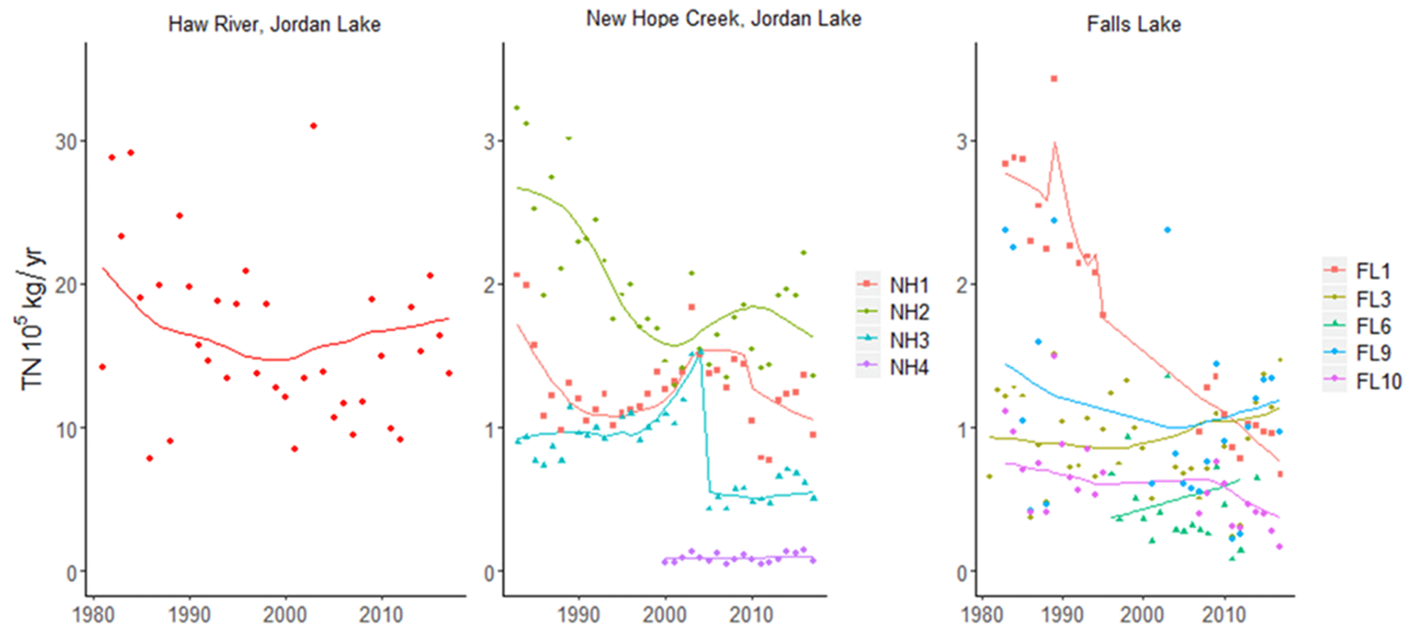
Figure 3 Weighted-regression on time, discharge, and season (WRTDS) annual nutrient loading estimates (points) and flow-normalized estimates (lines) for TN in the Haw River (HR) and New Hope Creek (NH) basins of Jordan Lake (JL) and Falls Lake (FL). For clarity, results are only shown for the most downstream load monitoring site (LMS) of each tributary to Jordan and Falls Lake. The only downstream LMS for Haw River is HR1. WRTDS loading estimates for other LMSs are provided in the Supplement (Fig. S4).

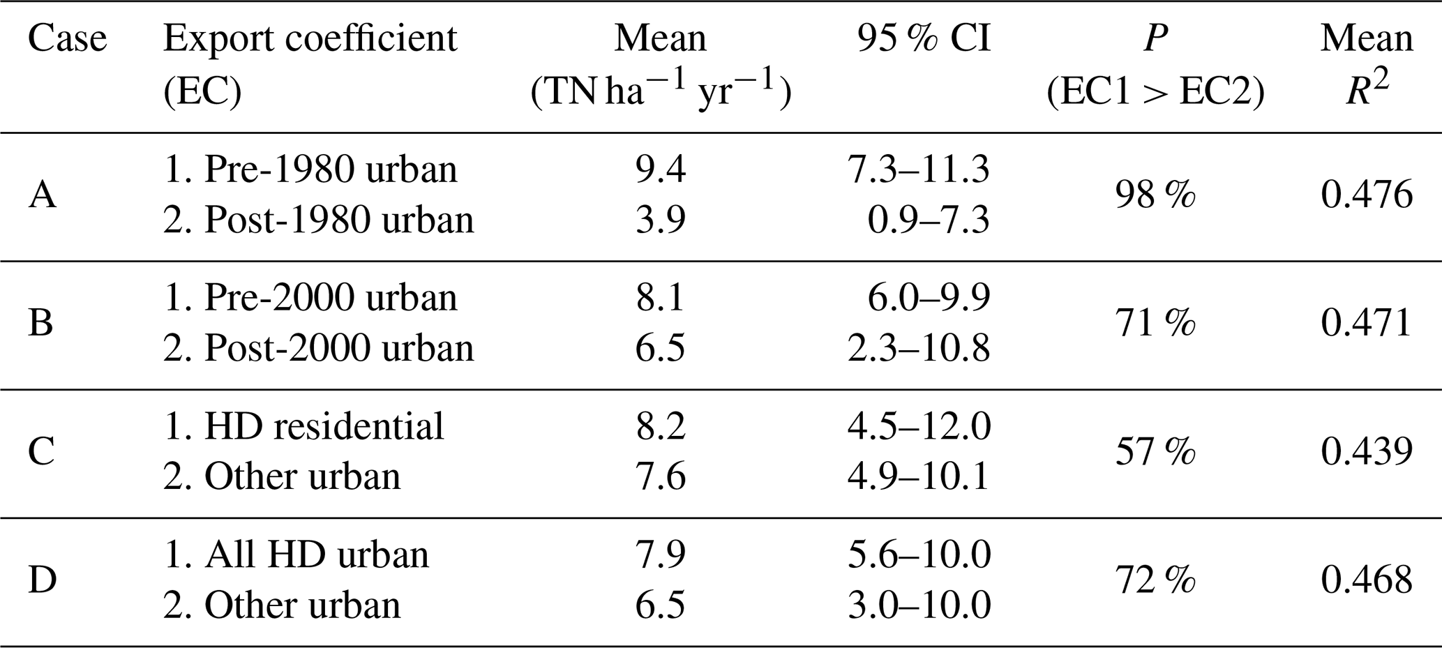
Table 2 Posterior means and 95 % credible intervals (CIs) of urban export coefficients (ECs) split by age and development density (low-density (LD) vs. high-density (HD) urbanization). The probability (P) that older urban lands (or HD urbanization) export more nitrogen than other urban lands was calculated by comparing Bayesian posterior draws. R² represents the ability of the model to predict temporal variability of loading at each LMS. Mean R² was determined by averaging the R² of all 25 LMSs.

3.2 Comparing different urban land classifications

The hybrid watershed model explains the spatial and temporal variability of in-stream (WRTDS-derived) TN loads based on precipitation and nutrient source distributions. To explore urban TN sources in more detail, we compare the posterior parameter distributions of different classifications of urban land use that consider the age, density, and type of urban development (Table 2). We find that a classification based on a pre-/post-1980 split results in significantly different export rates, with the pre-1980 urban lands exporting more than twice the amount of post-1980 urban lands. Here, “significantly different” implies a >95 % probability based on samples from the joint posterior parameter distribution. In addition, the pre-/post-1980 division leads to the highest R² values for individual LMSs. None of the other urban splits result in significantly different parameter estimates. However, export rates from high-density and older urbanization are consistently higher than the less dense and newer urban lands. Among the two splits based on density, combining high-density residential, industrial, and commercial lands has higher predictive power than just separating high-density residential from other urbanization (R²=0.47 vs. 0.44; Table 2).

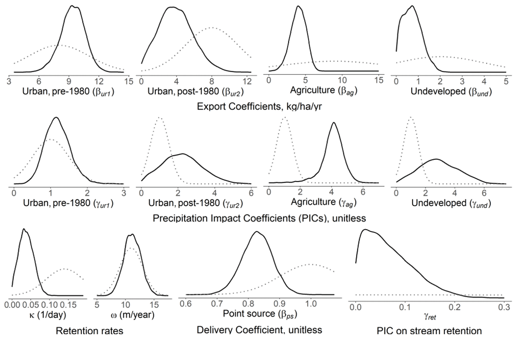
Figure 4 Prior (dotted lines) and posterior (solid lines) distributions for selected model parameters. Note that priors and posteriors are provided for all parameters in Tables 3 and S3.

3.3 Model posterior parameter estimates

The posterior ECs (β_x) of the preferred model (with the pre-/post-1980 urban split) show that urban and agricultural lands both contribute substantial TN per hectare (Table 3; Fig. 4). In particular, pre-1980 urban development exports 9.4 kg ha⁻¹ yr⁻¹ of TN (coefficient of variation (CV) of 11 %; Table 3), while post-1980 development exports 3.9 kg ha⁻¹ yr⁻¹ (CV = 41 %). Agriculture also contributes a substantial 4.0 kg ha⁻¹ yr⁻¹ (CV = 21 %), while undeveloped lands export a relatively low 0.7 kg ha⁻¹ yr⁻¹. In addition to pre-1980 urban export being significantly greater than other forms of development, undeveloped land has significantly less export than all developed lands, despite having a high CV (50 %; Table 3). Model posterior distributions indicate that parameter uncertainties are reduced substantially relative to the prior distributions (Fig. 4), consistent with Strickling and Obenour (2018), who found that priors had a relatively small influence on parameter estimates relative to the data (i.e., the likelihood).

Table 3 Mean posterior parameter estimates for export and delivery coefficients (β; EC, DC), retention rates (κ, ω), and precipitation impact coefficients (γ; PIC) along with 95 % credible intervals (CI). Note that subscripts are same as defined in Eq. (4).

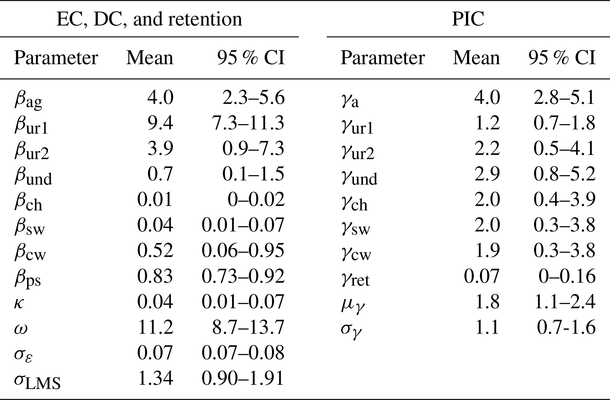
Land use ECs represent expected nutrient export for a year with mean annual precipitation (i.e., ${\stackrel{\mathrm{̃}}{p}}_{i,t}=\mathrm{1}$; Eq. 5a). Because the relationship between export and precipitation is nonlinear, the export coefficients represent median (but not mean) loading rates. The precipitation impact coefficients (PICs) can be used to calculate TN export during low- and high-flow years. Agriculture has the largest PIC (4.0; Table 3), implying that export from agricultural lands (crop and pasture) varies the most due to rainfall. During a high-flow year (90th percentile ${\stackrel{\mathrm{̃}}{p}}_{i,t}=\mathrm{1.18}$), nutrient export for agriculture would almost double from 4.0 to 7.7 kg ha⁻¹ yr⁻¹. For a low-flow year (10th percentile ${\stackrel{\mathrm{̃}}{p}}_{i,t}=\mathrm{0.81}$), nutrient export for agriculture (1.7 kg ha⁻¹ yr⁻¹) is less than half the median export. Pre-1980 urban lands show the lowest variation due to precipitation, ranging from 81 % of median export in low-flow years to 122 % in high-flow years.

3.4 Spatial variation in nutrient export and retention

The TN export from nonpoint sources is calculated for each subwatershed (Fig. 5a) using mean precipitation and mean posterior land and livestock ECs (β_ec; Table 3). Since the most intensive nutrient export comes from pre-1980 urban lands, subwatersheds intersecting the urban cores of major cities (Fig. 5a) have the largest expected export. Predominantly rural watersheds export between 1–3 kg ha⁻¹ yr⁻¹ of TN, while urban cores export over 6 kg ha⁻¹ yr⁻¹.

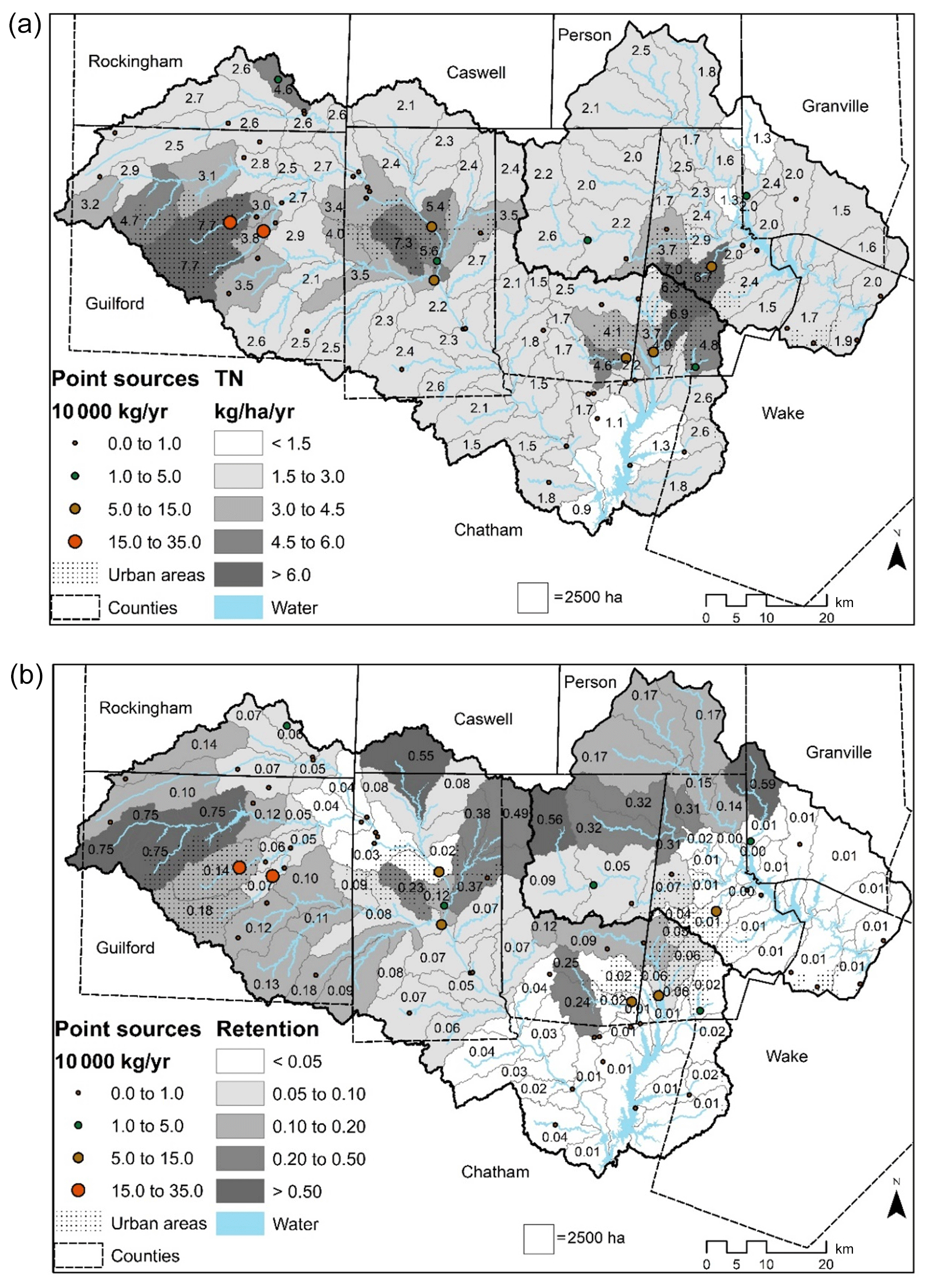
Figure 5 TN export (a) from land use and livestock by subwatershed; fraction of TN export from each subwatershed that is retained (b) in streams and reservoirs prior to reaching Jordan and Falls Lakes. Point source loads are shown separately as dots.

On average, 13 % of TN is retained within streams and waterbodies (Fig. 5b). Little TN is retained in subwatersheds close to JL and FL and along higher-order streams, while large TN removal rates (>70 %) occur for subwatersheds located upstream of reservoirs in the upper northwest portions of the JL basin. Overall, more TN retention occurs in reservoirs than in streams. Residence times and hydraulic loading rates are also affected by precipitation as modulated by the PIC for stream retention (γ_ret; 0.07; Table 3). For 1 SD increase in yearly precipitation (17.1 cm), expected stream residence times and hydraulic loading rates decrease roughly 7 % (Table 3; Eq. 7a and b). During low-precipitation years (lower 33 %), 15% of TN is retained in the JL and FL networks, while 12 % is retained during normal and high-precipitation years (upper 67 %).

Watershed-level random effects account for unexplained spatial variations in nutrient loading. For example, the negative random effects for small watersheds comprised of mostly pre-1980 urban development (NH7, NH8, FL2) imply these watersheds export less TN (−2.5, −1.8, and −1.2 kg ha⁻¹ yr⁻¹, respectively; Fig. S5) than typical pre-1980 urban lands (9.4 kg ha⁻¹ yr⁻¹; Table 3). Similarly, two LMSs (FL6, FL9) located directly downstream of large impoundments had negative random effects, implying these impoundments may be particularly efficient at trapping nutrients. On the other hand, three watersheds (NH1, HR5, and FL1) located just downstream of major WWTP discharges have elevated TN watershed-level effects, suggesting loads may be underestimated by the available point source data (Fig. S5).

Figure 6 Total nitrogen export by year and major basin separated by source. The star (^*) represents the total TN load that reached Jordan or Falls Lake.

3.5 Nutrient source allocations over time

Yearly TN loadings from 1994–2017 are reported based on mean model parameters, land use, livestock counts, and precipitation. Only the NH watershed shows a clear downward trend in TN loading, which appears to be largely driven by WWTP discharge reductions (Fig. 6). In both the HR and FL watersheds, annual loadings nearly tripled from the lowest- to highest-precipitation years due to high levels of agricultural lands which substantially increase export during wet years (Fig. 6). This high level of interannual variation makes it difficult to distinguish any positive or negative trends in these basins over the study period. Additionally, model residuals show no noteworthy temporal trends (Fig. S6).

3.6 Model skill assessment

The full hybrid model, including random effects, explains 95 % of the variation in the WRTDS loading estimates at LMSs (Fig. S7). Discounting the random effects, the model still explains 93 % of TN loading variability. The model (with watershed-level random effects) explains 96 % of the variation in the HR, 92 % in NH, and 83 % in FL (Fig. S7), suggesting some spatial variability in model performance. In cross validation, the predictive ability of the model remains high, with the R² of the full TN model (without watershed-level random effects) dropping slightly from 93 % to 90 %. R² values are also reported for individual LMSs to characterize the model's ability to predict the temporal variability. These R² values range greatly from below 0 (FL2, JL2, JL7) to above 0.80 (JL4, FL7, FL10) with a mean of 0.48 (Table 2).

4 Discussion

4.1 Nutrient export rates and discharge coefficients

In this study, we aim to enhance our understanding of nitrogen export, especially as it relates to land use and different types of urbanization. Variation in urban TN export has often been associated directly with population density (Bales et al., 1999; Burns et al., 2005; Line, 2013; Tetra Tech, 2014) or with proxies for density like net food imports (Hong et al., 2011; Sinha and Michalak, 2016). In this study, we compare variations in urban export due to the age of the urbanization versus different urban land covers (e.g., high- and low-density residential, commercial). Pre-1980 urban lands and high-density residential are moderately correlated in our study area (r²=0.64), yet Bayesian posterior parameter estimates show that exports from low- and high-density urban areas are not statistically different from each other. However, TN exports from pre- and post-1980 urban areas are significantly different (Table 2). This suggests that urban infrastructure age and historical development practices are more important than population density.

Various mechanisms, beyond density, could explain why older urban areas export more TN than recently constructed urban areas. Increased impervious connectivity in pre-1980 urban areas may lead to elevated runoff and nutrient washoff (Wollheim et al., 2005). In addition, pre-1980 urban development generally lacked stormwater management and erosion control measures (Howells, 1990; NC DEMLR, 2019). Therefore, streams in these areas have legacy sediments and often exhibit the urban stream syndrome with altered geomorphology and low biological health (Paul and Meyer, 2001; Bernhardt and Palmer, 2007; Miller et al., 2019), which can affect downstream nutrient loads and uptake (Meyer et al., 2005). Older neighborhoods are also likely to have larger trees and thus more leaf litter over impervious surfaces, which can also increase nutrient export (Janke et al., 2017). Finally, leaky sewer infrastructure in pre-1980 urban areas might be a substantial source of nutrients (Kaushal et al., 2011; Pennino et al., 2016) as compared to newer and more reliable infrastructure in post-1980 urban areas.

Model results indicate that post-1980 urban and agricultural lands exported similar amounts of nitrogen (3.9 and 4.0 kg ha⁻¹ yr⁻¹, respectively; Table 3). Our estimated agricultural export rate is lower than in previous studies (Dodd et al., 1992; Strickling and Obenour, 2018), which may be related to the fact that over 90 % of agricultural lands in our study area are pasturelands, rather than croplands (Falcone, 2015). Post-1980 urban export shows the most uncertainty in model posteriors (Table 3; Fig. 4). This might be due to the inconsistency of regulations being applied both temporally and spatially from 1980 to the present, and it might also indicate variation in the best management practices (BMPs) used in the region. Finally, undeveloped lands have very low export (0.7 kg ha⁻¹ yr⁻¹; Table 3) with moderate uncertainty (0.1–1.5 95 % interval; Table 3). This mean value is roughly 3 times lower than previous studies in the region (Tetra Tech, 2014; Strickling and Obenour, 2018).

Livestock export coefficients for chickens, swine, and cows (0.01, 0.04, and 0.50 kg yr⁻¹, respectively) imply that less than 1 % of the TN produced by these animals (i.e., 0.6, 9.9, and 54.8 kg an yr⁻¹, respectively; Ruddy et al., 2006) results in excess TN pollution in our study area. Overall, livestock-related nutrient export appears to account for <2 % of nutrient loading to the downstream reservoirs (Fig. 6; Table S4). Per hectare of agricultural land, livestock export averages just 0.5 kg ha⁻¹ yr⁻¹, about an order of magnitude less than the baseline agricultural land use export. It is important to note that livestock waste used to replace other (e.g., synthetic) fertilizers is generally represented by the agricultural land export. The livestock rates reported here represent TN export in excess of typical pasture and cropland export.

Our point source coefficient discounts WWTP loads by nearly 20 % (β_ps=0.83; Table 3). One potential explanation for this result is that TN from WWTPs (primarily nitrate) is processed and retained in stream networks more efficiently than TN from nonpoint sources. For example, increased denitrification rates have been observed downstream of WWTPs due to altered biochemical conditions (Wakelin et al., 2008; Rahm et al., 2016).

4.2 Interannual variability

Our analysis of interannual variability is facilitated through two enhancements to the hybrid watershed modeling approach of Strickling and Obenour (2018). First, we allow for retention to vary across years due to changes in precipitation, represented parsimoniously by a PIC for stream residence times and reservoir hydraulic loading rates (γ_ret; Eq. 7a and b). This modification produces a ±8 % variation in retention for ±1 SD change in annual precipitation. In this region, we find that the majority of retention occurs in reservoirs. Our mean stream retention rate (0.04 d⁻¹; Table 3) is comparable in magnitude to regional hybrid models (Strickling and Obenour, 2018; Gurley et al., 2019) but lower than previous watershed process models (Tetra Tech, 2014). Accurately quantifying stream retention rates is important to operators of WWTPs and regulators in order to accurately determine nutrient offsets for projects, which are often valued in millions of dollars (Jim Hawhee, NC DEQ, personal communication, 2020).

Second, we model the effects of precipitation variability on land use export using power functions (γ_x; Eq. 5) instead of linear relationships (Strickling and Obenour, 2018). The new formulation recognizes that as precipitation increases, its marginal effect on nutrient loading may intensify, as infiltration and evapo-transpiration rates are exceeded (Chin, 2013). Consistent with this explanation, agriculture has the highest PIC (4.0; Table 3), indicating that when annual precipitation is 20 % higher than the mean, TN export from agricultural lands will approximately double. On the other hand, pre-1980 urban lands, which are substantially impervious, have the lowest PIC values and only export 24 % more TN for a 20 % increase in annual precipitation.

By compiling nitrogen loads throughout the major basins (1994–2017; Fig. 6), we can analyze interannual trends and variability in TN sourcing. Interannual variation is large ($\sim \mathrm{3}\times$ difference from lowest to highest year) in both HR and FL, yet NH loadings show relatively little variation. This is due to high percentages of agricultural lands in HR and FL, which have the highest PICs. NH loadings, in contrast, are dominated by pre-1980 urbanization (lowest PIC) and point sources. By separating TN loadings into their sources, we are able to identify trends in specific nitrogen sources that could help inform management of individual watersheds. For example, though loadings in the NH watershed appear to decline over the study period from 6×10⁵ to 4×10⁵ kg yr⁻¹, this trend was driven by a nearly 50 % reduction in point sources (4×10⁵ down to 2.1×10⁵ kg yr⁻¹). At the same time, loading attributable to post-1980 urbanization increased almost 2-fold, from 0.2×10⁵ up to 0.4×10⁵ kg yr⁻¹ (Fig. 6).

4.3 Potential nutrient reductions

Model results strongly indicate that the majority of nutrient inputs to JL and FL are from anthropogenic sources. Based on identified sources of TN in the watershed, four management strategies would potentially lead to large nutrient load reductions: (1) reduction of point source loadings (i.e., WWTPs), which remain the largest individual source of TN, (2) retrofitting or replacing infrastructure in older urban environments (i.e., pre-1980 urban), which are the largest nonpoint source of TN per unit area, (3) mitigating TN loading from agricultural lands, especially during wet conditions, and (4) limiting, reducing, or offsetting the removal of undeveloped land, which have the lowest export.

The effectiveness of these nutrient control strategies will vary across different hydrologic conditions. For example, point sources are responsible for 44 % of TN loadings to JL and 14 % to FL from 1994 to 2017. However, these percentages rise to 55 % and 24 %, respectively, during dry years (Table S4). On the other hand, agricultural TN export accounts for 18 % of JL loadings and 30 % of FL loadings during normal flow years, but those numbers increase to 27 % and 37 % during high-flow years (Table S4). Therefore, strategies aimed at mitigating point source loadings will affect lake loadings more in low-flow years, while agricultural strategies will have a larger effect in high-flow years.

Undeveloped lands have the lowest nutrient export of all land-use sources (Table 3), which is consistent with findings from targeted water quality monitoring recently done in JL (NC Policy Collaboratory, 2019). However, undeveloped areas are decreasing in this region (1.5, 3, and 2 km² yr⁻¹ in HR, NH, and FL basins, respectively, from 1995 to 2015). Even though more recent development (post-1980) has significantly lower TN export when compared to pre-1980 development, it still exports approximately 6 times more TN than undeveloped lands (3.9 kg ha⁻¹ yr⁻¹ vs. 0.7 kg ha⁻¹ yr⁻¹; Table 3). At the same time, post-1980 urban export rates are similar to agricultural rates, implying that new urban construction in agricultural areas may have limited impact on total nutrient loading.

4.4 Summary and future directions

To efficiently manage watersheds, it is critical to identify the major sources and locations of pollutant loading under varying hydroclimatological conditions. We enhanced and applied a hybrid watershed modeling approach within a Bayesian framework to characterize TN loading rates from point and nonpoint sources and tested different classifications of urban land. By modeling interannual variability, we assessed how land use change and hydroclimatological variations have affected nutrient loading over time. Process-based and hybrid modeling approaches (e.g., SPARROW; Gurley et al., 2019) have been widely used to determine nitrogen loading rates, but these applications are often limited by an inability to capture interannual variations in loading and/or provide holistic parameter calibration with uncertainty quantification. Compared to previous Bayesian hybrid watershed modeling studies (Qian et al., 2005; Wellen et al., 2012; Strickling and Obenour, 2018), this study advances our ability to account for interannual variability in both export and retention. The study also discriminates how export rates vary across a relatively large number of sources (four land uses, three livestock types, and point sources). Our ability to resolve 18 process-based parameters within the Bayesian framework is facilitated, in part, by a relatively dense stream monitoring network and modern tools for Bayesian inference (Monnahan et al., 2017). The efficacy of the proposed approach for characterizing nutrient export in larger but less densely monitored watersheds could be explored in future research.

In this study, we identify areas of elevated TN export. In particular, we find that pre-1980 urban areas are hot spots for nonpoint TN loading. In addition, watershed-level random effects help identify outlier watersheds that export significantly more or less TN than the source distribution data would otherwise imply. Great costs have been incurred to protect waterways in the last 30–40 years without a clear understanding of how effective current policies have been in reducing nutrient loading (Parr et al., 2016; Utz et al., 2016). Our results suggest that post-1980 construction and land development BMPs have helped to reduce TN loadings from the built environment. We hope these findings will stimulate further research into the specific mechanisms that result in lower TN export from newer development. Enhancing the hybrid model with BMP and wastewater infrastructure data, in addition to more detailed land use and hydrography data, could be one approach for refining our understanding of how specific development practices influence watershed-scale nutrient loading. Given that even newer (post-1980) development is found to increase TN export by a factor of 5 or more, relative to undeveloped lands, further efforts are required to understand and mitigate the adverse impacts of urban development on nutrient loading.