the Creative Commons Attribution 4.0 License.
the Creative Commons Attribution 4.0 License.
 | 18 Jan 2021
Ubiquitous increases in flood magnitude in the Columbia River basin under climate change
Laura E. Queen
Philip W. Mote
David E. Rupp
Oriana Chegwidden
Bart Nijssen
The USA and Canada have entered negotiations to modernize the Columbia River Treaty, signed in 1961. Key priorities are balancing flood risk and hydropower production, and improving aquatic ecosystem function while incorporating projected effects of climate change. In support of the US effort, Chegwidden et al. (2017) developed a large-ensemble dataset of past and future daily streamflows at 396 sites throughout the Columbia River basin (CRB) and selected other watersheds in western Washington and Oregon, using state-of-the art climate and hydrologic models. In this study, we use that dataset to present new analyses of the effects of future climate change on flooding using water year maximum daily streamflows. For each simulation, flood statistics are estimated from generalized extreme value distributions fit to simulated water year maximum daily streamflows for 50-year windows of the past (1950–1999) and future (2050–2099) periods. Our results contrast with previous findings: we find that the vast majority of locations in the CRB are estimated to experience an increase in future streamflow magnitudes. The near ubiquity of increases is all the more remarkable in that our approach explores a larger set of methodological variation than previous studies; however, like previous studies, our modeling system was not calibrated to minimize error in maximum daily streamflow and may be affected by unquantifiable errors. We show that on the Columbia and Willamette rivers increases in streamflow magnitudes are smallest downstream and grow larger moving upstream. For the Snake River, however, the pattern is reversed, with increases in streamflow magnitudes growing larger moving downstream to the confluence with the Salmon River tributary and then abruptly dropping. We decompose the variation in results attributable to variability in climate and hydrologic factors across the ensemble, finding that climate contributes more variation in larger basins, while hydrology contributes more in smaller basins. Equally important for practical applications like flood control rule curves, the seasonal timing of flooding shifts dramatically on some rivers (e.g., on the Snake, 20th-century floods occur exclusively in late spring, but by the end of the 21st century some floods occur as early as December) and not at all on others (e.g., the Willamette River).
- Article
(6275 KB) - Full-text XML
- BibTeX
- EndNote


Among natural disasters in the Pacific Northwest (PNW), flooding ranks second behind fire in federal disaster declarations1 since 1953 despite extensive flood prevention infrastructure. The largest flood in modern times on the Columbia River occurred in late spring (May–June) 1948 and obliterated the town of Vanport, which lay on an island between Portland, OR, and Vancouver, WA, permanently displacing its 18 500 residents2. Other disruptive floods in the region include the Heppner flood in 1903, one of the deadliest flash floods in US history (Byrd, 2014); floods on the Chehalis River in both December 20073 and January 20094 that closed Interstate 5, the main north–south transportation corridor through the Pacific Northwest, for several days each time at a cost of several millions of dollars per day to freight movement alone; and floods on the Willamette River in February 1996 and April 2019. The timing of typical floods varies widely across the region: low-elevation basins in western Washington and Oregon typically flood in November through February, whereas the snow-dominant basins east of the Cascades more typically flood in spring, sometimes as late as June (Berghuis et al. 2016).
The Columbia River drains much of the Pacific Northwest, with the fourth-largest annual streamflow volume in the USA and a drainage that includes portions of seven states plus the Canadian province of British Columbia (BC), an area of 668 000 km2 (Fig. 1). Its numerous federal and nonfederal dams provide flood protection, hydropower production, navigation, irrigation, and recreation services. A treaty between the USA and Canada, signed in 1961, codified joint management of the river's reservoirs (and funded construction of new reservoirs in BC), primarily to provide flood protection and hydropower production5. The USA and Canada have entered negotiations to update the treaty; the USA's “key objectives include continued, careful management of flood risk; ensuring a reliable and economical power supply; and improving the ecosystem in a modernized Treaty regime.” (ibid.) Both countries have expressed an intention to include the effects of climate change on streamflows, and clearly a key aspect of hydrologic change is to inform the treaty negotiations of the influence of climate change on the magnitude of flooding.
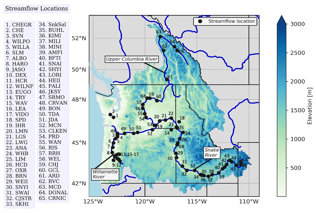
Figure 1Domain of hydrologic simulations used in this paper, with colors indicating elevation of each grid cell, major rivers highlighted in blue, and numbers indicating locations of streamflow points highlighted in Figs. 6–11 and Table 1. See Chegwidden et al. (2017, 2019) for all streamflow locations plotted in Fig. 5.
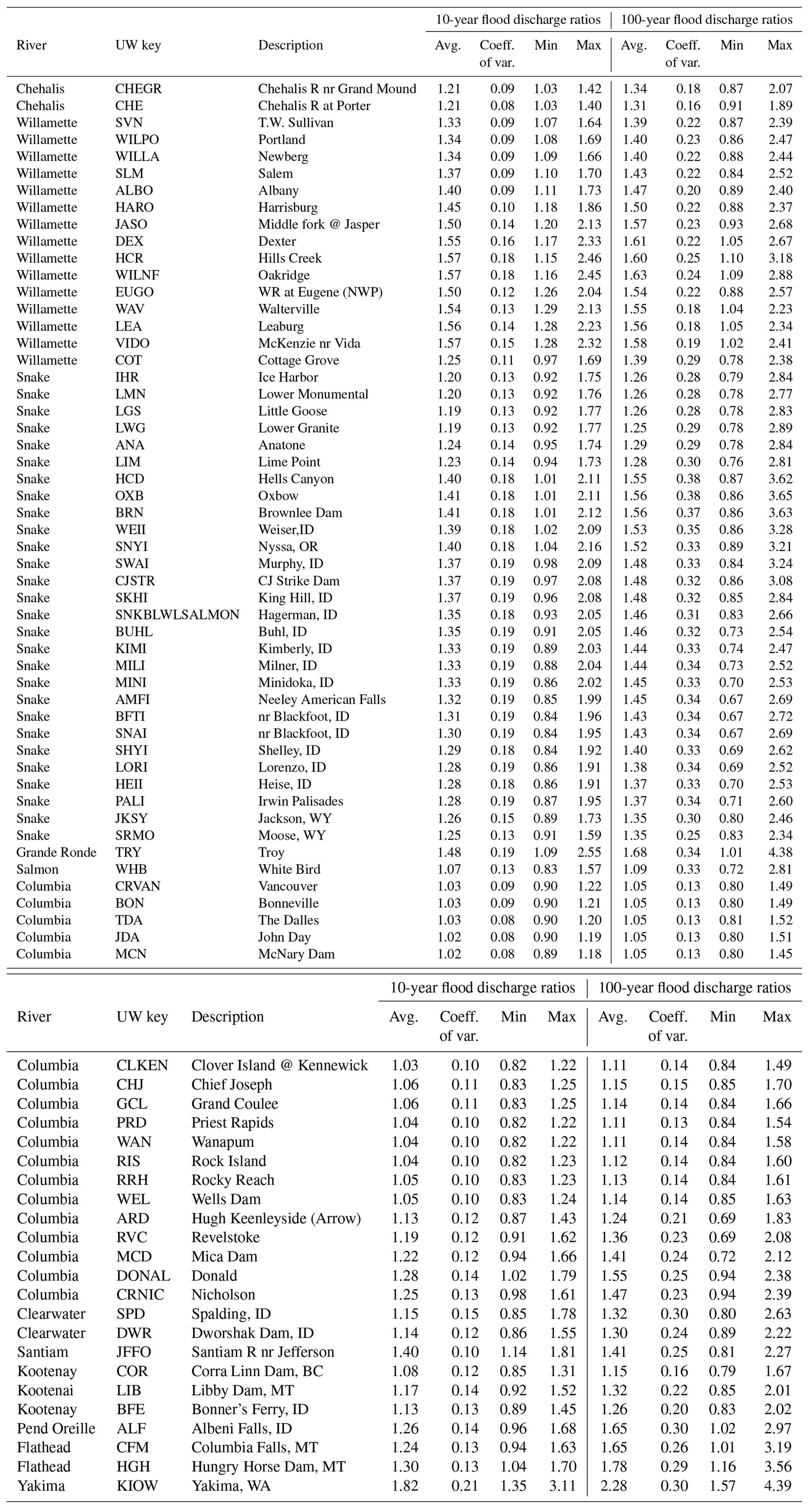
Table 1Information about locations featured in this paper – location, river, and discharge ratios.
While rising temperatures potentially affect all parts of the hydrologic cycle, in a snowmelt-dominated hydrologic system such as many of the Pacific Northwest's river basins, warming directly affects snow accumulation and melt (e.g., Hamlet et al., 2005). Observational studies have shown consistent changes toward lower spring snowpack (Mote et al., 2018), earlier spring streamflow (Stewart et al., 2005), and lower summer streamflow (Fritze et al., 2011) since the mid-20th century. Observations of trends in flooding in the USA have generally failed to find any consistent trends (Lins and Slack, 1999; Douglas et al., 2000; Sharma et al., 2018). Sharma et al. (2018) offer several possible explanations, chiefly “decreases in antecedent soil moisture, decreasing storm extent, and decreases in snowmelt”. The detection of trends in floods is complicated by the interaction of extreme events and nonstationarity (Serinaldi and Kilsby, 2015). Moreover, as a result of the substantial alteration of rivers to prevent flooding (e.g., by the construction of dams and levees) during the observational period, the best long-term records – i.e., on streams with the least modifications – are on rivers that were not producing sufficiently disruptive floods to lead decision-makers to construct flood protection structures. That is, as flooding of settlements, infrastructure, or other assets led to the investments in flood protection structures on most rivers, thereby altering the streamflow regime and dividing any gauged records into pre- and post- modification, the ones that were left unmodified tended to be small and/or remote.
To interpret the ambiguous results from observed trends, Hamlet and Lettenmaier (2007) used the Variable Infiltration Capacity (VIC) hydrologic model forced twice with detrended observed daily weather for the period 1916–2003, with about 1 ∘C of temperature difference between the two. They then compared 20- and 100-year flood quantiles for basins at varying sizes in the western USA and found a wide range of changes in flood magnitude ranging from large decreases to large increases (±30 %). Broadly, the responses depended somewhat on basin winter temperature, with the coldest basins (<−6 ∘C) showing reductions in flood magnitude owing to reduced snowpack, basins with moderate temperatures exhibiting a wide range of changes, and rain-dominant (>5 ∘C) basins showing little change, though the warm basins in coastal areas of Washington, Oregon, and California showed increased flood magnitude.
Modeling work using state-of-the-art hydrologic models has been applied to understand where and how flood magnitudes may change in the future. Tohver et al. (2014) found widespread increases in flood magnitudes, especially in temperature-sensitive basins (mainly on the west side of the Cascades), but their approach used monthly global climate model (GCM) output, so changes in daily precipitation would not be represented. Salathé et al. (2014) used a single GCM, the ECHAM5, linked to a regional climate model to obtain high-resolution (in space and time) driving data for VIC over the period 1970–2069. As did Hamlet and Lettenmaier (2007), they compared the ratio of flood change (2050s vs. 1980s) against mean historical winter temperature and found a majority of locations with a higher 100-year flood, in some cases by a factor of 2 or more; while they projected increases in every one of the warmer basins (>0 ∘C), a substantial fraction of colder locations had decreases in flood magnitude.
Chegwidden et al. (2019) describe the process used to generate the streamflow ensemble used here. In addition, they used analysis of variance (ANOVA) to analyze the different influences of choices of emissions scenario (as a Representative Concentration Pathway – RCP), GCM, internal (unforced) climate variability, downscaling method, and hydrologic model, and how those influences varied spatially across the domain and also seasonally and by hydrologic variable. They found that the RCP and GCM had the largest influence on the range of annual streamflow volume and timing, and the hydrologic model had the largest influence on low streamflows. The hydrologic variables they considered were snowpack (maximum snow water equivalent (SWE) and date of maximum SWE), annual streamflow volume, centroid timing (the date at which half the water year's streamflow has passed), and seasonal streamflow volume; primary focus was on centroid timing, annual volume, and minimum 7 d streamflow. They did not examine high-flow extremes that can lead to flooding. The purpose of this paper is to address this important gap in our understanding of the future Pacific Northwest hydrology; to do so, we use the largest available ensemble of climate–hydrology scenarios. By using a large ensemble, we ensure a reasonable breadth of climatic and hydrological futures in order to better describe the range of possible future flooding and how it varies across the region with its diverse hydroclimates. We also note possible shortcomings associated with modeling future flooding.
2.1 Hydrologic modeling dataset
To assess changing flood magnitudes under climate change, we analyzed changes in water year maximum daily streamflows in a large ensemble of streamflow simulations at 396 locations in the Columbia River basin (CRB, Fig. 1) and select watersheds in western Oregon and Washington (Chegwidden et al., 2017). The simulations were constructed from permutations of modeling decisions on forcing datasets and hydrologic modeling. Specifically, choices included 2 RCPs (RCP4.5 and RCP8.5), 10 GCMs, 2 methods of downscaling the climate model output to the resolution of the hydrologic models, and 4 hydrologic model implementations, for a total of 160 permutations. For our analysis, we extracted a more tractable dataset of 40 simulations per location, by only considering simulations with RCP8.5 and the multivariate adaptive constructed analogs (MACA) downscaling method (Abatzoglou and Brown, 2012).
The rationale for using a subset of the available data is as follows. First, the time-dependent set of greenhouse gas concentrations in RCP4.5 is fully included in RCP8.5, so any concentration of greenhouse gases on the RCP4.5 path can be converted to a point on RCP8.5 (at a different time). We analyzed results for both RCP8.5 and RCP4.5, and found that to first order the changes in flood magnitude in RCP4.5 were approximately 2∕3 those in RCP8.5, which is also roughly the ratio of global temperature change over the period considered (IPCC Summary for Policymakers, 2014). For clarity we show only the results for RCP8.5. Second, we considered only simulations using the MACA downscaling method because of the method's ability to capture the daily GCM-simulated meteorology critical for assessing changes in extremes and its skill in topographically complex regions (Lute et al., 2015). The other downscaling approach used by Chegwidden et al. (2019), the bias correction and statistical downscaling (BCSD) method (Wood et al., 2004), produces probability distributions of daily precipitation inconsistent with the GCM response to forcings because the method stochastically disaggregates monthly data to daily data based on historical statistical properties of the daily data. This statistical property limits the ability of BCSD to reproduce changes in storm frequency in the future, making it a less attractive choice for daily extreme streamflow analysis (Hamlet et al., 2010; Guttman et al., 2014).
Model output used in this study came from the following 10 GCMs: CanESM2, CCSM4, CNRM-CM5, CSIRO-Mk3-6-0, GFDL-ESM2M, HadGEM2-CC, HadGEM2-ES, INMCM4, IPSL-CM5A-MR, and MIROC5. These 10 GCMs were chosen primarily for their ability to accurately reproduce observed climate metrics during the historical period mainly of the northwestern USA but also at sub-continental and larger scales as assessed in Rupp et al. (2013) and RMJOC (2018). The four hydrologic model implementations originated from two distinct hydrologic models: the Variable Infiltration Capacity (VIC; Liang et al., 1994) model and the Precipitation Runoff Modeling System (PRMS; Leavesley et al., 1983). VIC and PRMS are process-based energy balance models and were both run on the same 1∕16th-degree grid with output saved at a daily time step for the period 1950 to 2099. VIC is a macroscale semi-distributed hydrologic model that solves full water and energy balances, and in these simulations it also included a glacier model (Hamman and Nijssen, 2015). Three unique implementations of VIC were used with independently derived parameter sets (P1, P2, P3) marked by differences in calibrated parameters, calibration methodology, and meteorological and streamflow reference sets. PRMS is a distributed, deterministic hydrologic model which, in contrast to VIC, does not allow for subgrid heterogeneity; see Chegwidden et al. (2019) for details. It is important to note that these hydrologic simulations and calibrations do not include reservoir models and have not been calibrated for daily, let alone maximum daily, flows, and these shortcomings may affect the results.
2.2 Flood magnitude
We assessed changes in flood magnitude in the Columbia River basin by comparing water year maximum daily streamflows over a 150-year period (1950–2100). We estimated the 10, 5, 2, and 1 % probability of occurrence (commonly referred to as the 10-, 20-, 50-, and 100-year flood, respectively) by fitting generalized extreme value (GEV) probability distributions to simulated water year maximum daily streamflows for 50-year windows of the past (1950–1999) and future (2050–2099) periods; see Fig. 2 for an example. (We also looked at 30- and 75-year windows, choosing 50 years as a balance between sample size favoring longer periods and nonstationarity considerations favoring shorter periods.) We used Python's scipy.stats.genextreme module (Jones et al., 2001) to fit a Gumbel distribution and estimate flood magnitudes for each return period. We assessed change in flood magnitude as the “discharge ratio” of the estimated future to past floods for a given return period; a ratio greater than 1 indicates an increase in flood magnitudes, while a ratio less than 1 indicates a decrease.

Figure 2Generalized extreme value (GEV) fit of annual maximum daily streamflow from 50 years of simulation using output from one GCM (HadGEM2-ES) and one hydrologic model (PRMS) for the Willamette River at Portland. Blue and red dots and lines indicate the annual values and GEV fit for the 1950–1999 “past” and 2050–2099 “future” periods, respectively.
We describe how changes in flood magnitude vary by climatic zone across the PNW by using an efficient and internally consistent proxy for climatic zone: the centroid of timing – the day in the water year by which half the annual volume of water has passed the stream location. The centroid of timing is a metric of snow dominance (e.g., Stewart et al. 2005) which is related to the spatial distribution of temperature and tends to decrease downstream. This temporal proxy of a hydrologic characteristic is effective in the Columbia River basin, where most of the precipitation occurs in winter and the relative magnitude and timing of the freshet from the spring thaw is a good indicator of the importance of snowmelt to streamflow. An early centroid indicates that rain – which falls predominantly during the cooler, earlier part of the year – is the driver of the peak streamflows at the location, while a late centroid indicates that snowmelt during later spring months is the prime hydrological driver. We computed the centroid using the 1950–1979 simulated years. Note that Chegwidden et al. (2019) also used the change in centroid as a hydrologic variable of interest; below, we discuss our results in the context of their findings.

Figure 3Comparison of 10-year (a, b, c) and 100-year (d, e, f) flood magnitudes from the observationally derived NRNI and the 40 climate–hydrologic model simulations, for 1950–2008, for select locations on the rivers as shown.
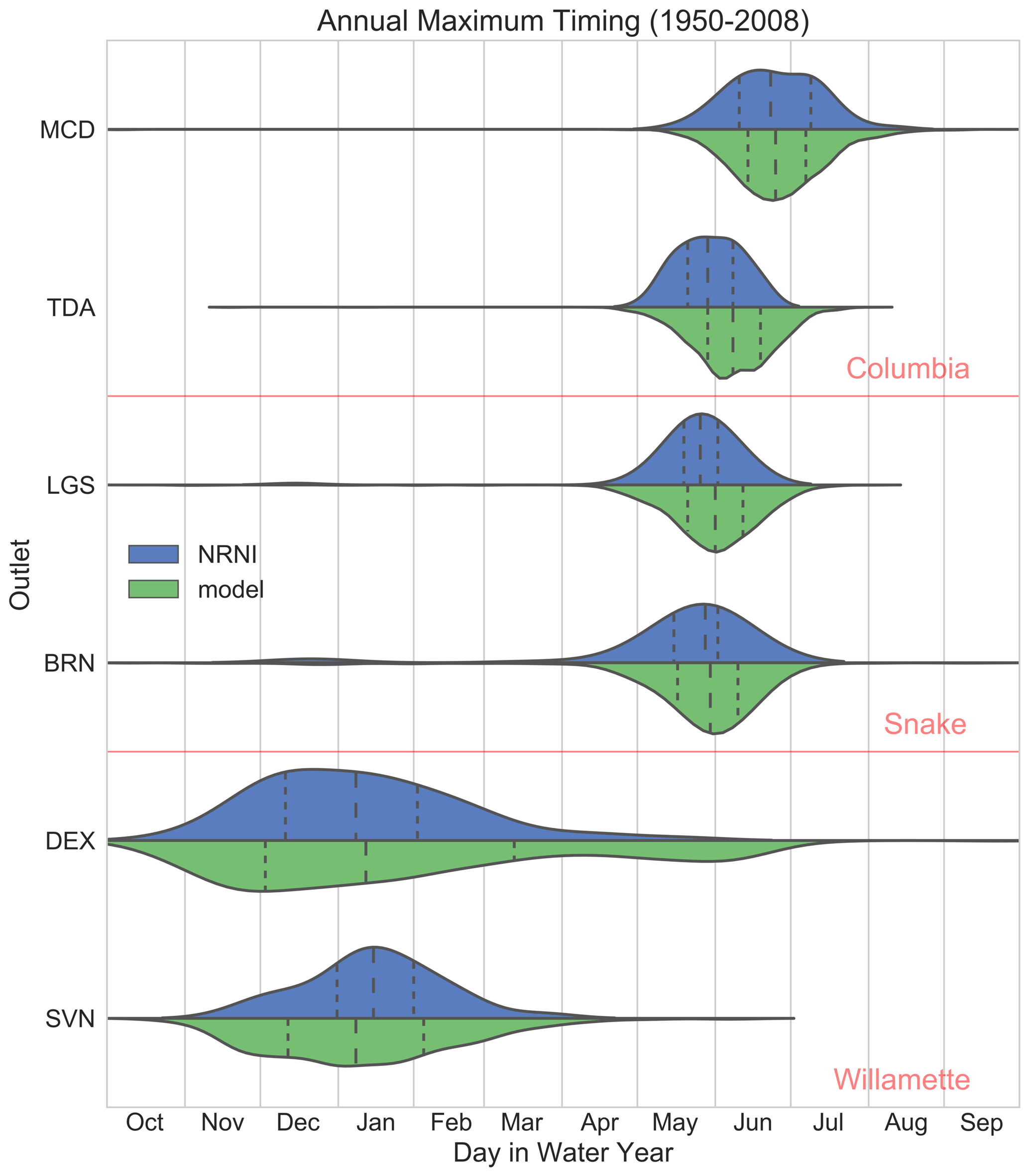
Figure 4Statistical representations of the variation through the water year of the timing of flood events, 1950–2008, for NRNI (blue) and the 40 simulations of 1950–2008 with the climate–hydrology modeling system (green). To create each curve, the dates of the five highest streamflows in the period of record are tallied, and the resulting distributions smoothed. Long dashed lines indicate median date; short dashed lines indicate the lowest and highest quartiles. MCD: Mica Dam (upper Columbia River); TDA: The Dalles (lower Columbia River, between the confluences of the Snake and Willamette rivers); LGS: Little Goose (lower Snake River); BRN: Brownlee; SVN: T. W. Sullivan (lower Willamette River near Portland); DEX: Dexter (Middle Fork Willamette River).
2.3 Model evaluation
Comparing directly between gauged flows and modeled flows is inadvisable since the observed streamflows are substantially altered by regulation, which is not accounted for in the hydrological model. However, a set of streamflows called No Reservoirs No Irrigation (NRNI; River Management Joint Operating Committee, 2018) has been developed by federal agencies to support practical analysis. The NRNI dataset exists at ∼190 sites across the Columbia River basin for the years 1928–2008, and streamflows are adjusted to correct for reservoir management and the diversions and evaporation associated with both the reservoirs and irrigated agriculture. This dataset is suitable for comparisons with our modeling setup, and we have computed return period curves using GEV fits at all the NRNI locations (not shown) for the period common to both NRNI and our ensemble, viz, 1950–2008. From these fits we have estimated the 10-year and 100-year values (Fig. 3). On the lower main stem Columbia River (Fig. 3a and d), the return period curves are very close to those computed from NRNI, and the means of simulations are almost all within 8 % of the NRNI values. Individual hydrologic model configurations are not consistently biased across the basin nor across return periods; despite its different provenance, PRMS generally lies within the return period streamflows of the three VIC configurations rather than being consistently different from all VIC configurations, although the lowest values are from PRMS. On the Snake River, the mean of modeled high streamflows ranges from 5 % above NRNI at Little Goose to 24 % above at Oxbow for 10-year floods (and 14 to 41 % for 100-year floods), but again no hydrologic model stands out as strongly biased. On the Willamette River, however, the modeled 10- and 100-year flood magnitudes lie almost entirely below NRNI, and the means are too low by 30 % (T. W. Sullivan, 10-year flood) to 50 % (Hills Creek, 100-year flood). PRMS and the P2 calibration of VIC are consistently closer to NRNI on the Willamette River. In general, the simulated flood statistics are least biased on larger river reaches where the hydrographs are less flashy. For the Columbia River main stem, modeled extremely high streamflows agree well with the NRNI dataset.
We also examined the ensemble performance for 1950–2008 in the distribution of timing of peak daily streamflow for 28 locations along the Columbia, Snake, and Willamette rivers (a subset is shown in Fig. 4). At all locations we examined, the median date (as well as earliest and latest quartiles) of annual maximum daily streamflow in the ensemble is within 10 d of the observed streamflow from NRNI. The modeled distribution is shifted slightly later than NRNI on the lower Columbia and slightly earlier than NRNI on the Willamette River. As with magnitudes, the agreement in timing suggests a robust modeling setup since the comparison tests the ability of the combined climate–hydrologic modeling system to match observed streamflow, constrained only by the broad physics of the climate system and by meteorological bias correction (which cannot substantially change the timing of the day of the year most conducive to high streamflows). Although the modeled streamflows are calibrated, the statistical approach to calibrations is not sensitive to the extreme maximum daily streamflow studied here.
It is worth stressing that these results compare outputs of hydrologic models in which the inputs are simulated daily weather (which is then bias-corrected) rather than observed daily weather, and that the hydrologic models are calibrated to 7 d means rather than the daily values relevant here. In other words, we are evaluating the ability of the combination of simulations of weather and hydrologic response. The weaknesses evident in Fig. 4 pose a note of caution in interpreting our results, but a full diagnosis of the causes of the shortcomings (especially on the Willamette River) is beyond the scope of this paper, as is the evaluation of our modeling system's performance at other locations besides these rivers.
3.1 Regional changes in flood ratio
Figure 5 shows the changes in maximum daily discharge for all of the 396 streamflow locations for different return periods. The horizontal position of each circle represents the centroid of timing. The circles are semi-opaque, so overlapping circles lead to a deeper saturation. Points on the same river are ordered from more to less snow dominant (i.e., right to left) traveling downstream; strings of circles in a smooth pattern usually indicate one of the larger rivers, highlighted in Fig. 6. Each circle in Figs. 5 and 6 represents an average of 40 simulations: 10 GCMs and 4 hydrologic model configurations.
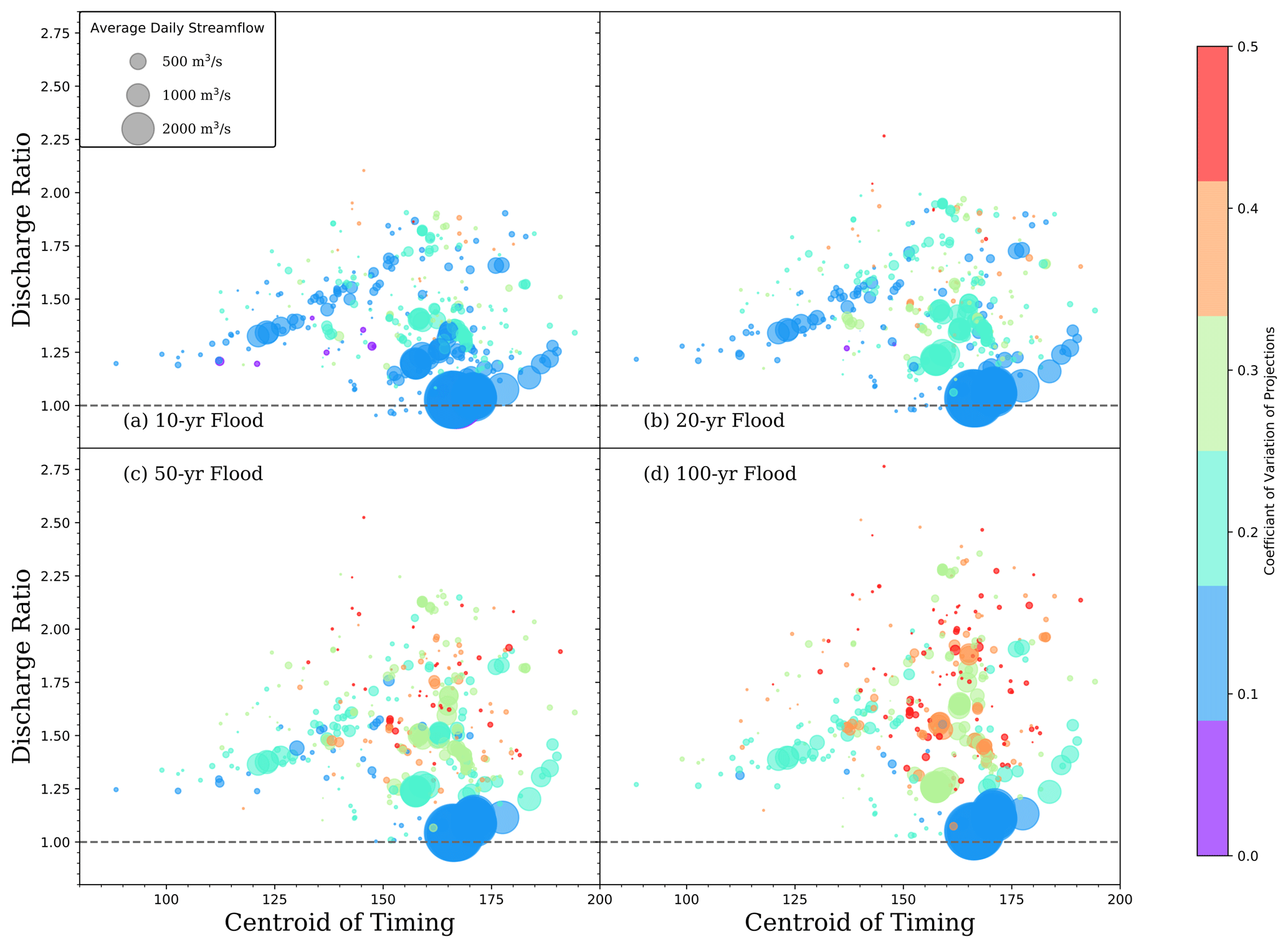
Figure 5Discharge ratios (future : past) versus centroid of timing (day on which 50 % of water year streamflow has passed, an indicator of snow dominance) for all 396 locations and 4 return periods. For each location, the average of 40 ensemble member ratios calculated from GEV distribution fitting from 50-year windows for the future (2050–2099) and past (1950–1999) time periods is shown. Points are sized by average daily streamflow and colored by the coefficient of variation of the 40 ratios.
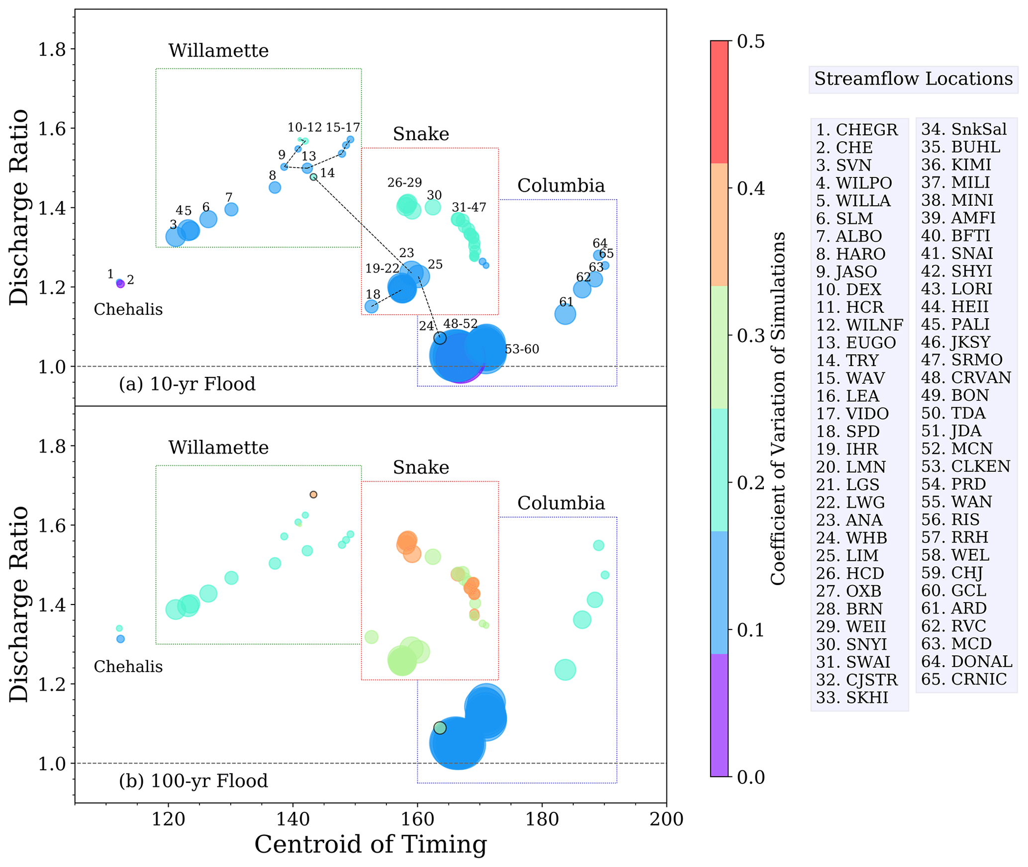
Figure 6As in Fig. 5 but only for points on the indicated rivers. Dashed lines indicate tributaries: 9–12 are on the Middle Fork Willamette River, and 15–17 are on the McKenzie River; tributaries of the Snake River are the Grande Ronde (14), Clearwater (17), and Salmon (24) rivers. In (b), the Grande Ronde and Salmon rivers are clearly distinguished by a black circle around their perimeter. Table 1 translates the codes in the legend into named locations and shows the numerical values represented in the figure. As is evident from both snow dominance and size, locations are ordered downstream to upstream from left to right for each river.
A striking result in Fig. 5 is that, in contrast to the results of Tohver et al. (2014), the flood magnitude increases (i.e., the discharge ratio exceeds 1) at nearly every streamflow location and return period (though not for every individual climate scenario, as shown in Fig. 7). Broadly, the patterns are similar across all return periods though with slightly higher ratios for longer return periods, and subsequent figures will show only the 10- and 100-year floods. For the streamflow locations with centroid <125 or so (i.e., 2 February), flood ratios are fairly concentrated about 1.25 for all return periods. For mixed rain–snow basins, roughly delineated by centroids between 125 and 160 (8 March most years), flood ratios range widely from just below 1 to about 2.4 for the 10-year and 3.2 for 50- and 100-year floods. For the longer return intervals, there is a wide range of projected changes in daily flood at many locations (indicated by the red coloring). This is undoubtedly partly due to the GEV fit extrapolating from 50 to 100 years. Finally, for the basins with streamflow centroid >160, the ratios have a smaller range, from slightly greater than 1 to a maximum that increases from about 2 for the 10-year to about 2.75 for the 100-year flood. Tohver et al. (2014) distinguished basins by their DJF temperature, a rough proxy for our snow dominance metric, and found a substantial number of locations where the flood ratio for both the 20-year and 100-year flood was as much as 20 % lower for the 2040s compared with a historical period. We return to this point in the conclusions.
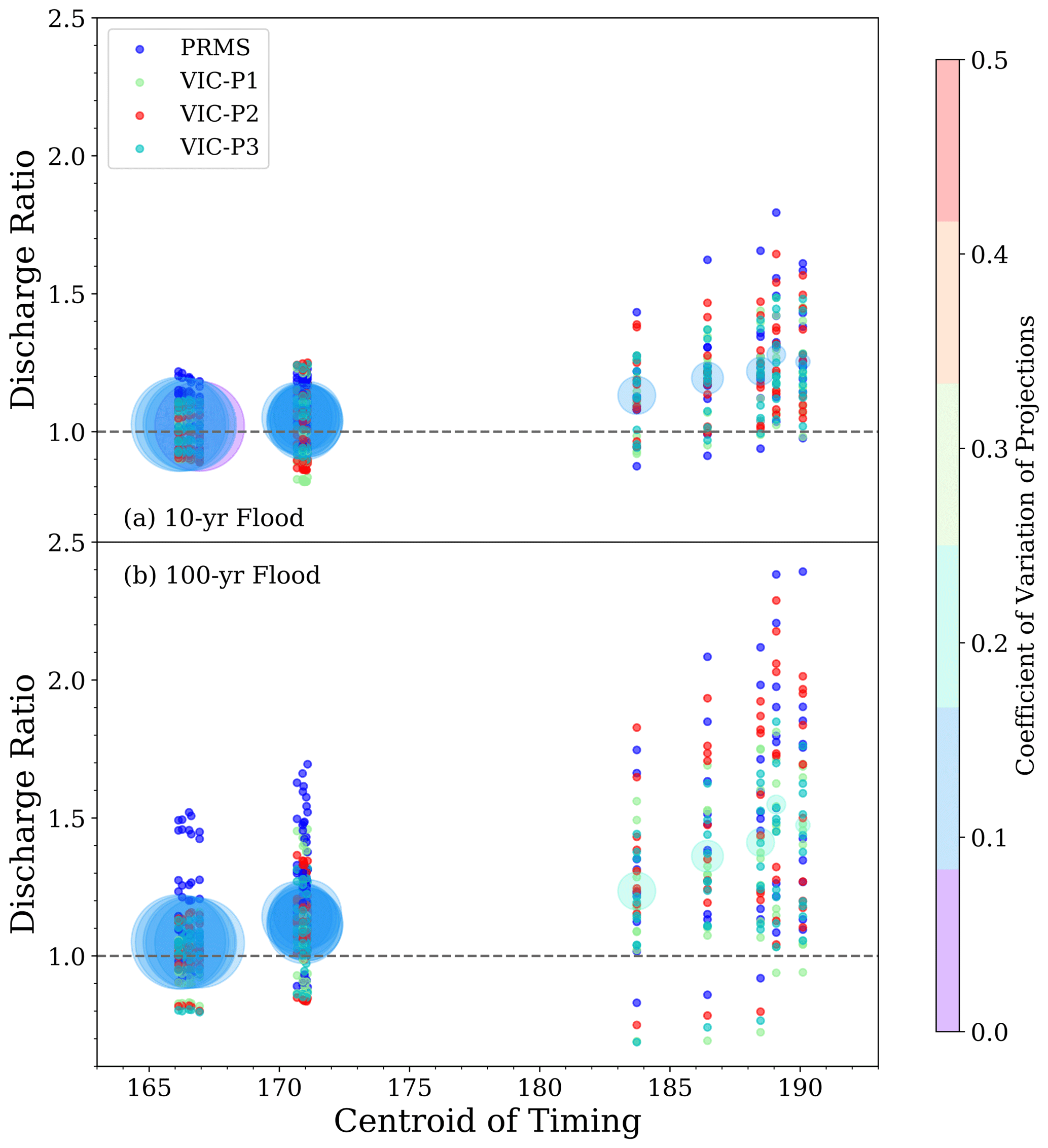
Figure 7Averaged (large circles) and individual ensemble member (small colored circles) discharge ratios for simulated streamflow locations along the main stem Columbia River for the 10-year (a) and 100-year (b) return periods. As shown in the legend, the color of the dots distinguishes results by hydrologic model setup.
To understand better how flood magnitude changes along the length of a river, we focus (Fig. 6) on a handful of significant rivers in the region – the main stem Columbia, Willamette (along with major tributaries the McKenzie River and Middle Fork Willamette River), and Snake rivers – and also on the Chehalis River in southwest Washington (see Introduction). Flow locations and select numerical results are listed in Table 1. Many of the larger tributaries also have streamflow points in our dataset, so we can infer the role of tributaries in changing the flood magnitudes in the future, as discussed below. The Columbia River includes the most snow-dominant basins, with a centroid of >190 d (early to mid-April) in the Canadian portion of the basin. The flood ratio decreases almost uniformly along the length of the river, from 1.3 for the 10-year and >1.5 for the 100-year period in the Canadian portion to just above 1 at the last few points along the river (The Dalles, Bonneville, and Portland). Past flood events on the main stem Columbia River are exclusively associated with large spring snowmelt, and the large tributaries (the Yakima, Snake, and Willamette rivers) contribute annual streamflow volume but rarely contribute peak streamflow at the same time; as shown below, the future flood timing changes, but flood magnitudes change little in the lower Columbia River owing to the fact that the Columbia River integrates such diverse hydroclimates. Like the Columbia River, the Willamette River also has flood ratios that decrease along the length of the river as it integrates more diverse hydroclimates, from 1.7 to 1.35 for both return periods. The McKenzie River (points 15–17), one of the three tributaries that converge at Eugene to form the Willamette River, is a highly spring-fed river with higher baseflow than is represented in the hydrologic models, though it is unclear how that difference would manifest in the flood statistics. Nonetheless, the combination of an important unrepresented process and the large errors in flood magnitudes relative to NRNI (Fig. 3) is potentially problematic for simulating future changes in flooding.
In contrast to the Columbia and the Willamette rivers, the Snake River behaves oppositely: flood ratio increases downstream along the length of the river, until the confluence with the Salmon River, which drains a large mountainous area of central Idaho. On parts of the Snake the ratios are as high as 1.4 for 10 years and 1.6 for 100 years. Then after the confluence with the Salmon River, which has much lower change in discharge ratio, the ratios on the Snake River drop to about 1.2 for 10 years and about 1.3 for 100 years. Our hypothesis is that in the Snake River above the Salmon River the tributaries shift from snow dominant to rain dominant, so that a single storm can drive large rainfall-driven increases (possibly with a snowmelt component), leading to larger synchronous discharges. The Salmon and Clearwater rivers retain less exposure to such shifts and dilute the effects of single large storms on flooding.
Each circle in Figs. 5 and 6 represents an average of 40 simulations: 10 GCMs and 4 hydrologic model configurations. To better understand the range in results, Fig. 7 shows the discharge ratio for all 40 simulations at each point on the main stem Columbia River. Although the mean flood ratio at the lowest two points is only barely above 1, several ensemble members have ratios less than 1, and a few have ratios > 1.5. Moving upstream, the range in results increases, as shown also by the color of the dots.
3.2 Dependence of results on modeling choices
As in Chegwidden et al. (2019), we separate the results – here for the three largest rivers – into variations across GCM (Fig. 8) and variations across hydrologic model configurations (Fig. 9). The ranking of flood ratios by GCM changes substantially between basins and even within a basin, and it does not correspond to the changes in seasonal precipitation. For the upper Columbia River, the models with the least warming – INMCM4 and GFDL-ESM2M (Rupp et al., 2017) – have almost no change in flood magnitude, but the HadGEM2-ES, which warms considerably in summer, produces a large decrease in flood magnitude. In the Willamette and Snake rivers, the range of projected flood changes by different GCMs remains large from the headwaters to the mouth of the river, whereas for the Columbia River the range diminishes considerably as one moves downriver.
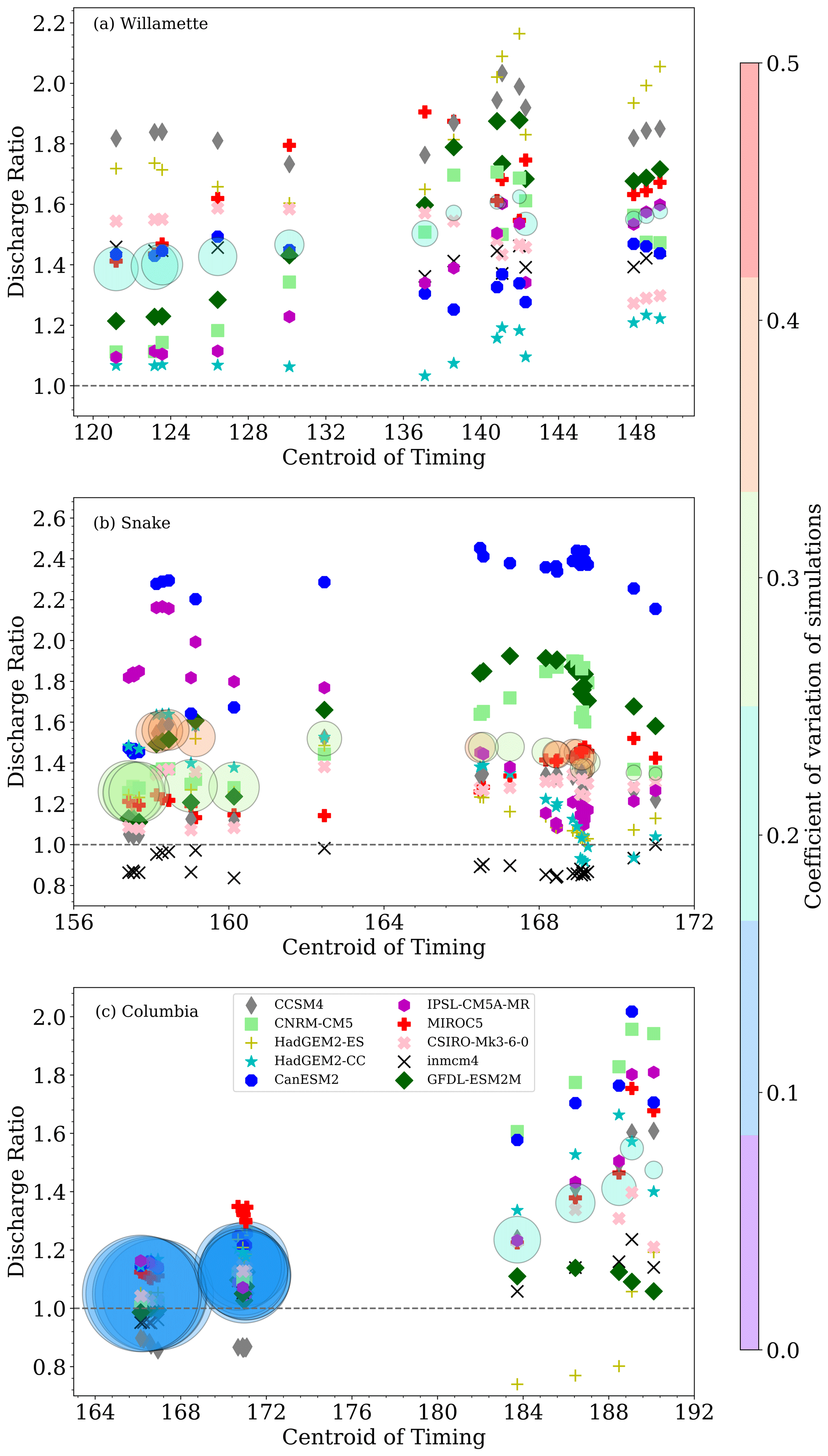
Figure 8Average ratios of all 40 ensemble members (large circles) and the average of 4 hydrologic model results for each GCM (symbols), shown for simulated streamflow locations along the Willamette River (a), Snake River (b), and main stem Columbia River (c) for 100-year return periods. GCMs are ordered in the legend by their ranking in Rupp et al. (2017), representing their ability to simulate Pacific Northwest climate.
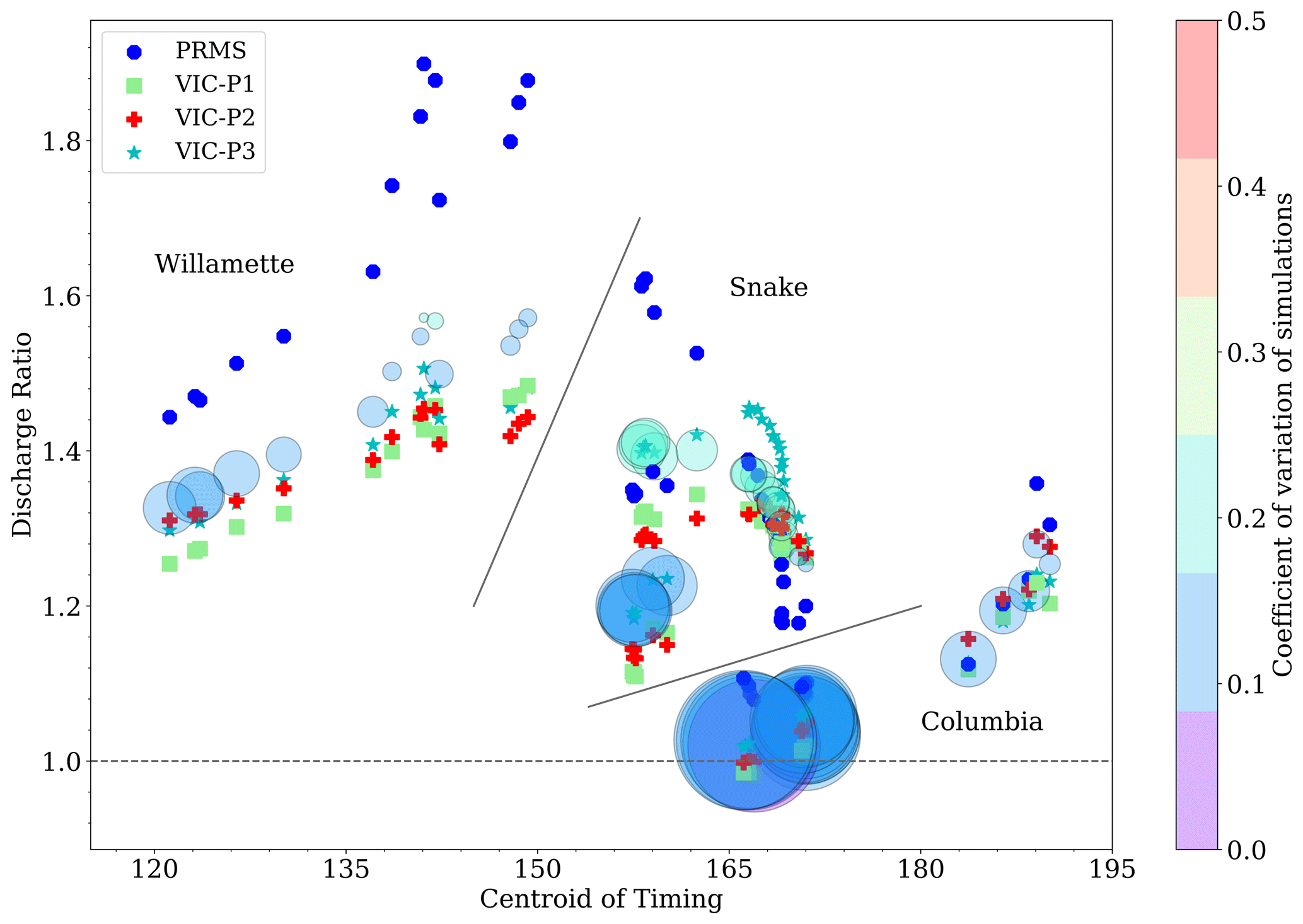
Figure 9As in Fig. 8 but averaged by hydrologic model, for 10-year return period, and combined into one panel.
The variation of results depends less on hydrologic model than on GCM (Fig. 9), though the differences across hydrological models are still substantial. For the Willamette, lower Snake, and both upper and lower Columbia rivers, the PRMS model predicts substantially larger increases in flooding than the three calibrations of the VIC model. For the upper Snake River, it predicts substantially smaller change than any VIC calibration. While it is perhaps not surprising that the three calibrations of VIC are close to each other, it is striking just how different the projections are from PRMS at most locations on these three rivers. Chegwidden et al. (2019) found that the main contributors to differences in hydrologic variables (except low streamflows) generally were the climate scenarios (GCM and RCP), consistent with our findings here. (The order of models is similar in the equivalent figure for the 100-year return period, but we elected to show the 10-year figure since the 100-year figure is more difficult to decipher because the symbols overlap with those from other rivers.)
To parse the contributions of climate factors (represented by the GCMs) and hydrologic factors (represented by the hydrologic models), we perform ANOVA on the 40 discharge ratios. The pie charts in Fig. 10 show the proportion of the total variance explained by climate factors and hydrologic factors at different locations. For the Willamette River, the portion of uncertainty connected to the climate grows more important, and the portion of uncertainty connected to the hydrologic variability less important, going from the confluence of the three major tributaries at Eugene to the mouth. For the Snake and Columbia rivers, climate is responsible for virtually all of the variance in projections in the upper reaches, but only about half at the lowest point, similar to the Willamette River. The Willamette River basin is much smaller, and a large storm can affect the entire basin on the same day (Parker and Abatzoglou, 2016), whereas storms typically take a couple of days to move across the Snake and Columbia rivers (and generally move upstream). With larger and more diverse contributing areas, differences in the rates at which the hydrological models transfer precipitation to the point of interest become more important. Unlike Chegwidden et al. (2019), we did not attempt to isolate the response to anthropogenic forcing from internal climate variability. Though several techniques for separating these two factors have been used (e.g., Hawkins and Sutton, 2009; Rupp et al., 2017; Chegwidden et al., 2019), either these techniques are infeasible with our dataset or we question their suitability for the application to changes in extreme river flows.
3.3 Change in timing
Although in a broad hydrologic sense a flood is a flood regardless of what time of year it occurs, there are potentially significant ecological differences depending on time of year; for example, scouring the river bottom causes significant loss of salmon eggs (Goode et al., 2013). Moreover, water management policies are strongly linked to the calendar year (see Discussion). We computed the probability of flooding for (all 40) past and future simulations at all the points on the three rivers (Fig. 6) as a function of day of year (Fig. 11). For the Willamette River, no significant change in timing occurs; however, for the upper Willamette River, a single peak in likelihood in February becomes more diffuse. For the Snake River, all locations see a shift toward earlier floods, consistent with the transition to less snow dominant and more rain dominant. Whereas floods were historically concentrated in the period of mid-May to mid-July, the projected future flooding period spans December to June. For the Columbia River, the mode in the flood timing shifts earlier by half a month in the upper Columbia to about a month in the lower Columbia River. The distribution also broadens with an elongated tail towards winter such that there is low, but non-negligible, probability of floods occurring as early as January. The magnitudes of the 10- and 100-year flood events in the lower Columbia River are not projected to increase substantially (Figs. 6–9). However, the window during which a major flood could occur expands, with the likelihood of major flooding in May or April (or even as early as February) increasing.
Our study joins a small number of others in examining high-flow extremes using a large hydroclimate ensemble. Gangrade et al. (2020) used a similar ensemble approach, analyzing hydrological projections for the Alabama–Coosa–Tallapoosa River basin with 11 dynamically downscaled and bias-corrected GCMs (10 of which our studies share) and 3 hydrologic models (including VIC and PRMS). While they did not examine extreme daily streamflows, they did calculate changes in the 95th percentile of daily streamflow (Q95). Perhaps because of the hydroclimatic uniformity of that basin, they found very small differences in Q95 across hydrologic models, which contrasts with our results showing changes in flood magnitudes varying by watershed and distance downstream. Thober et al. (2018) conducted a similar study in some European river basins, but rather than using a climate ensemble they simply imposed uniform warming scenarios on a hydrologic model (i.e., a more straightforward temperature sensitivity analysis rather than an exploration of the range of future climate scenarios). Other, smaller ensemble studies of floods in different basins include Huang et al. (2018), with four GCMs and three hydrology models, and Vormoor et al. (2015) with several parameterizations of one hydrology model.
Returning to the Pacific Northwest, our findings contrast with earlier work. Salathé et al. (2014) found decreases in flood magnitude at a substantial number of sites, but our results show increases in flood magnitude at nearly every return period and location, which includes about 100 locations not included in their study. They also noted that directly downscaling the GCM outputs leads to a smaller range of results than when running the regional model as an intermediate step, so we infer that, if we had had access to regional climate model (RCM) simulations driven by all 20 of our RCP–GCM combinations, our range of results might have been larger. Another important difference may be in the spatiotemporal coherence of extreme precipitation, which in the RCM would be generated directly by the interaction of synoptic-scale storms, topography, and (to a small extent) surface water and energy balance, and in our study by the interaction of the GCM-scale synoptic storms and constructed analogs derived from observations. A large ensemble would reduce the magnitude of that effect. In our study, the MACA statistical downscaling approach preserves much of the daily variability from the GCM, so the primary reason for the difference between our results and theirs is probably the fact that we analyzed 40 scenarios. Some locations, for example the points on the lower Columbia River, had a handful of ensemble members with decreasing flood magnitude. But averaging the entire ensemble nearly always resulted in an increase in flood magnitude. It is possible therefore that their study, repeated with a larger ensemble of hydrologic–climate model combinations, might have found ubiquitous increases in flood magnitude as ours did.
Prior results (Hamlet and Lettenmaier, 2007; Tohver et al., 2014; Salathé et al., 2014) suggested a decrease in flood magnitude in snowmelt-dominated basins like that of the Columbia River, since reduced snowpack reduces the store of water available to be released quickly in a spring flood (like the May–June 1948 Vanport flood). In a subbasin of the Willamette River, Surfleet and Tullos (2013) projected decreases in flood magnitude for return periods >10 years in the Santiam River basin under a high-emissions scenario (SRES A1B, 2070–2099 vs. 1960–2010; eight GCMs), attributing the decreases to fewer large rain-on-snow events. Our results for the Santiam River show an increase of 40 % for both 10- and 100-year floods; this result includes rain-on-snow events, since they are represented in VIC, which computes the accumulation of water in the snowpack and determines whether sufficient energy has been provided to create a melt event. Our results point to ubiquitous increases in magnitude throughout the basin, even on the lower main stem Columbia River. We also project some large increases in flood magnitude in the coldest basins, including the headwaters of the Columbia River, suggesting that the former results were missing some key details. It seems likely that any reduction in flood magnitude originating from the warming-induced reduction in spring snowpack is offset by other factors. While there is evidence that warmer future temperatures could engender slower melt rates (Musselman et al., 2017), the effect on high-streamflow events is less clear. For example, Chegwidden et al. (2020) showed that magnitudes of both rain- and snowmelt-driven floods are likely to increase across headwater basins in the Pacific Northwest through the 21st century. These results emphasize the necessity of revisiting reservoir rule curves, which are strongly tied to historical hydrographs, and also emphasize that changes in the seasonality of flooding can be dramatically different from the changes in the mean hydrograph. In particular, in the lower Snake and lower Columbia rivers, changes in magnitude of flooding are modest, but changes in timing of the earliest quartile of flood events are much larger than the 0.5–1-month shift in the mean hydrograph.
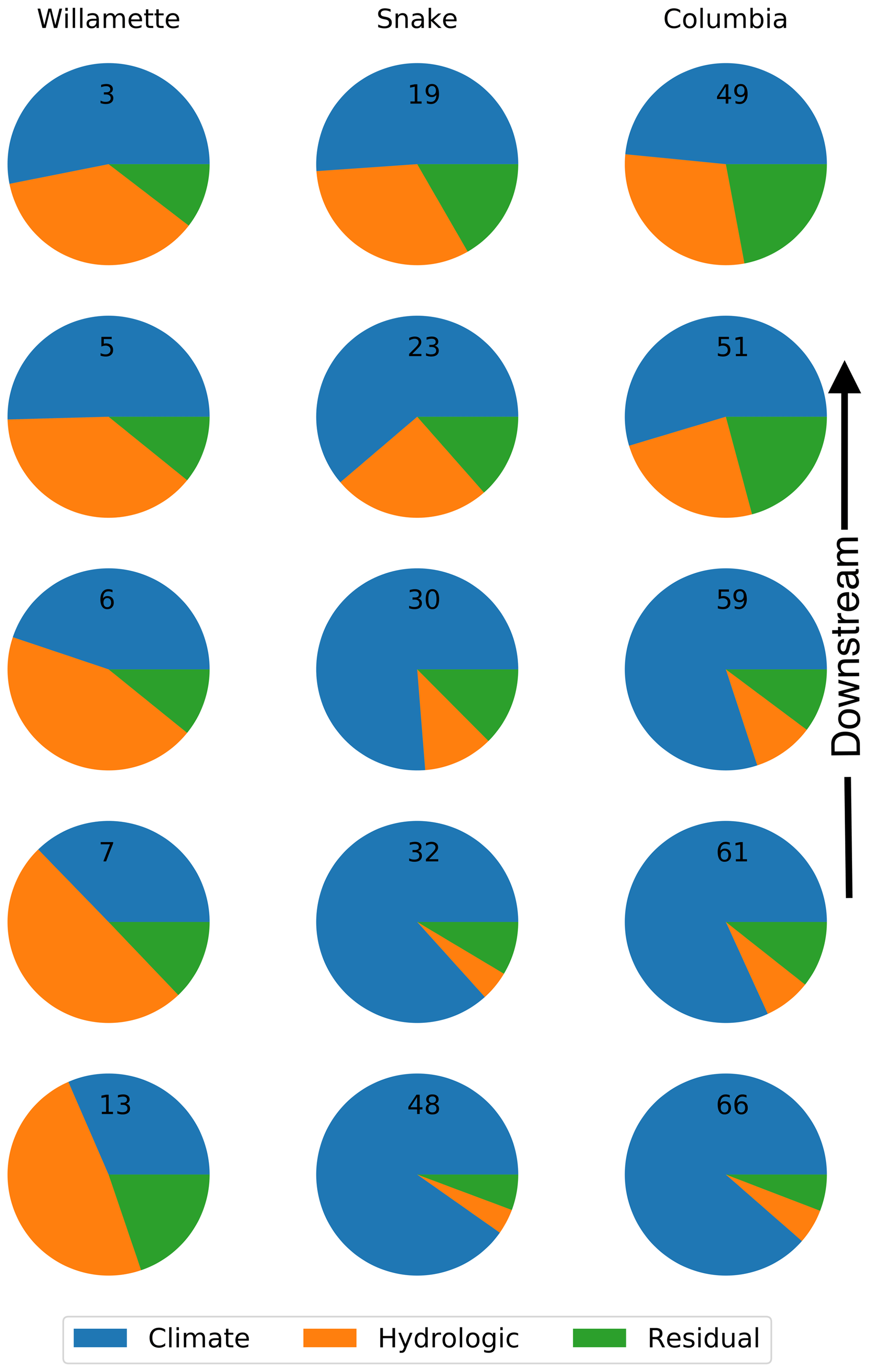
Figure 10ANOVA results for select locations on the indicated rivers, for climate and hydrologic factors (and the residual). Charts are numbered to correspond with their location in Fig. 6, with the most-downstream location at the top.
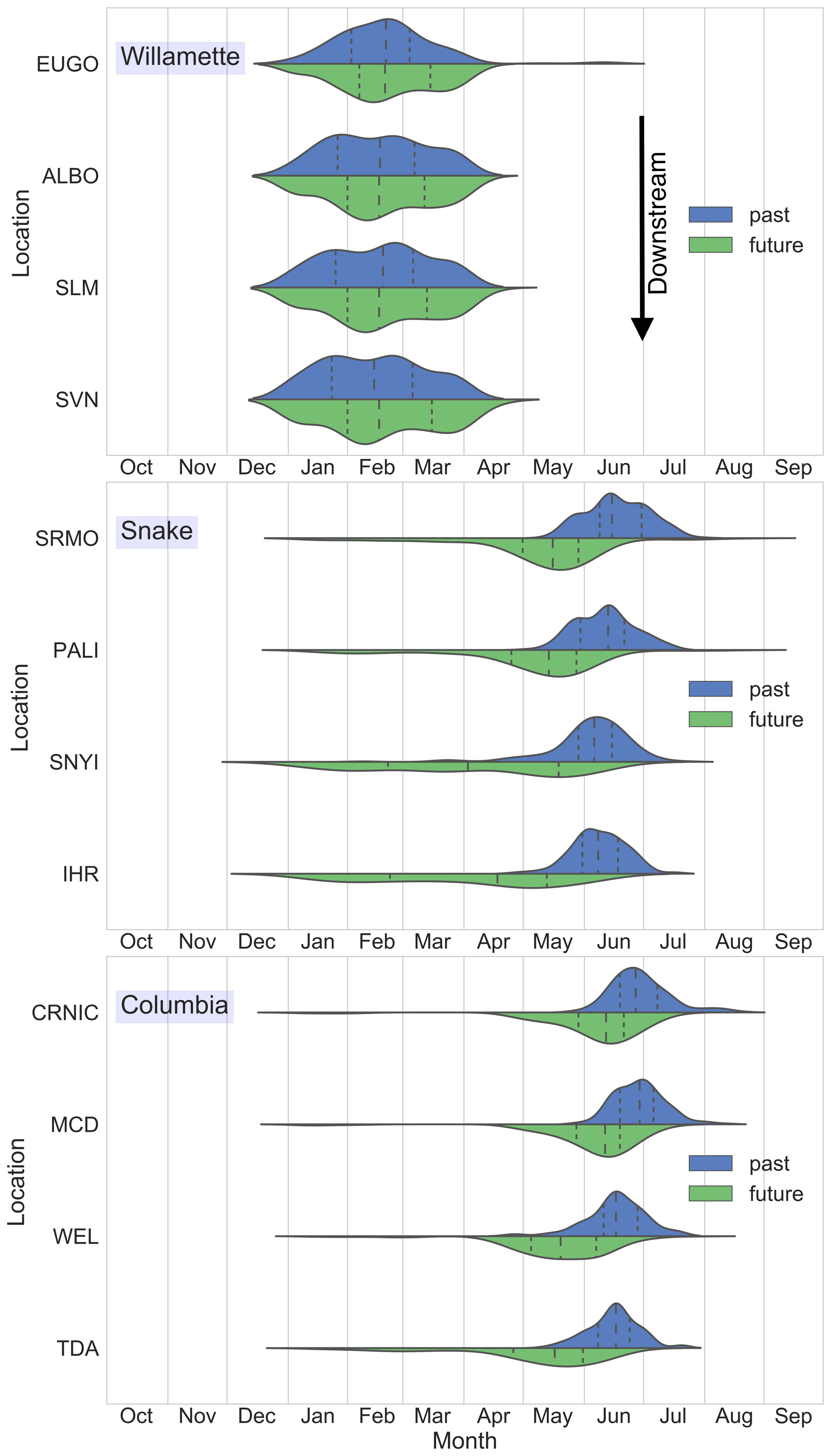
Figure 11Statistical representations of the variation through the water year of the timing of flood events. For each of the 40 simulations, the dates of the five highest streamflows in the 50-year past (blue) and future (green) windows are tallied, and the resulting distributions smoothed. Long dashed lines indicate median date; short dashed lines indicate the lowest and highest quartiles.
The evaluation of the modeling system in Sect. 2.3 raises some concerns about the reliability of our results, especially as to flood magnitude on the Willamette River main stem, and also in smaller basins where we have not performed an evaluation. While this is a concern in an absolute sense, in a relative sense our results are probably more robust than those of earlier studies in the Pacific Northwest, for several reasons. First, previous studies have rarely provided the sort of evaluation of flood statistics that we show in Sect. 2.3. Second, we used more methodological variations, which tend to broaden, not narrow, the spread of results, and yet we still obtained a narrowing of the spread of results to almost ubiquitous increases. Third, our use of a large ensemble samples a wide climate space by using GCMs as opposed to RCMs. Conventional wisdom and evidence from the weather and seasonal climate forecasting realms illustrate the utility of considering ensembles and that generally the true outcome of a prediction lies near the middle of the ensemble. Our ANOVA (Fig. 10) shows that climate scenarios contribute a majority of the variation among results for most of the basin. Consequently, it is of great importance to sample the climate scenarios broadly, which currently only GCMs can do. Large ensembles of RCMs are rare; the 12-member NARCCAP ensemble (six RCMs, four GCMs; Mearns et al., 2013), some of whose model runs were completed a decade ago, remains the largest but has a spatial resolution of only 50 km. CORDEX North America similarly now has a comparable-size ensemble, but mostly still at 50 km (some at 0.22∘), and was not available in such large numbers when we began our hydrologic simulations. At such spatial resolutions, RCMs would still have to be further downscaled and bias-corrected for use in our hydrologic models (∼6 km spatial resolution). In the trade-off between breadth of climate scenarios and spatial resolution, these ensembles offer insufficient improvement in spatial resolution relative to our GCM ensemble to justify sacrificing the breadth in climate scenarios represented by choosing just four GCMs. While RCMs certainly have their place in such work and were used in some previous studies, using GCMs in this study allowed for a larger climate space to be sampled, thus adding to the robustness of our results.
Although the likeliest outcome, as shown in Fig. 7, is for smaller changes in flood magnitude in the lower Columbia River than elsewhere, a prudent risk management strategy would consider the range of possibilities. The validation (Figs. 3 and 4) provides no a priori basis for excluding or under-weighting the projections from any hydrologic model. On the Willamette River, a rain-dominant basin, our hydrologic simulations of flood magnitudes are biased low; possible causes for the low bias originate both in the climate and hydrological models. For example, a low bias in extreme daily precipitation may lead to an underestimation of the hydrologic response. We also note that the hydrologic models were calibrated to 7 d means rather than daily values and may underestimate the daily response in smaller basins. Nevertheless, three physical processes contribute directly to the increase in magnitude: an increase in seasonal precipitation affecting soil saturation, an increase in extreme daily precipitation, and a warming-induced reduction in the snow-covered area in the wet season. In our results for the Willamette River this reduction in snow-covered area reduces the buffering effect of snow accumulation during storms and more than offsets an increase in melt from rain-on-snow events. This mechanism is supported by Chegwidden et al. (2020), who, using the same underlying dataset as our study, project a growth in both prevalence and magnitude of rain-driven floods at the expense of floods from snowmelt and rain-on-snow events.
Our findings provide an initial indication of how existing flood risk management could respond to a warming climate. Reservoir management is guided by rule curves which are intended to reflect the changing priorities and risks during the year. For example, reservoirs used for flood control have rule curves that require reservoir levels to be lowered when approaching the time of year when flood likelihood increases, and reservoir levels may be raised as the likelihood decreases. For the Willamette River, we found little change in the distribution of timing of flood events, which indicates that, with the state of the science today, reservoir rule curves may need to be altered according to magnitude of flooding (which our results indicate will increase by 30–40 %) but not timing; a reservoir model, along with further investigation of the low bias in observed flood magnitudes (Fig. 3e and f), would be required for a complete understanding of how flood risk (magnitude and timing) will actually change. For the Snake River, larger shifts in the timing imply a need to completely re-evaluate the existing rule curves. For the Columbia River, the mode in flood timing shifts earlier by half a month in the upper Columbia to about a month in the lower Columbia River. The distribution also broadens, with an elongated tail towards winter such that there is low, but non-negligible, probability of floods occurring as early as January. These changes in timing imply a need for moderate alteration of rule curves for reservoirs in the Canadian portion of the Columbia River basin.
Our results should not be taken as a precise prediction of flood magnitude change but rather as the best available projections given the current state of the science. Two important factors need to be considered when interpreting our results: first, in using RCP8.5, we selected the most extreme scenario of rising anthropogenic greenhouse gas concentrations. If efforts to stabilize the climate before 2050 are successful, the flood magnitudes shown here will undoubtedly be smaller (our analysis suggests most of the locations would see a change in flood magnitude about 1∕3 smaller for RCP4.5; e.g., a ratio of 1.3 (30 % increase) for RCP8.5 would correspond to a ratio of 1.2 for RCP4.5).
The second important factor in interpreting our results is that the actual river system in the Pacific Northwest includes many dams, a majority of which have flood control as a primary (or at least a top) objective. As a result, actual streamflows (and the changes in streamflow) at a given point in the river would be altered by reservoir management. Translating these changes in flood magnitude into actual changes would require a reservoir model for the basin or subbasin of relevance. One could then compute optimal rule curves for the major flood control reservoirs (perhaps time-evolving every couple of decades, to reflect the likely changes in scientific understanding and emissions trajectory). Even without that additional analysis, however, our results stress that the magnitude and/or timing of flood events will change throughout the basin. In other words, what worked for flood control in the past will not work as well in the future.
This study may have some utility in framing and quantifying the possible changes in flood risk as the Columbia River Treaty is in renegotiation, but further work would be needed to assign probabilities to future flood magnitude. Such work includes (a) a deeper understanding of the underlying model differences to explain differences in model sensitivities (our analysis in Sect. 2.3 shows that PRMS performs about as well as the three calibrations of VIC for simulating past peak streamflows, but more work would be needed to understand the reasons for divergence in future projections), (b) applying different statistical and/or dynamical downscaling methods, and (c) using a more sophisticated approach to evaluating extremes in a nonstationary climate (as advocated by Serinaldi and Kilsby, 2015). The mechanisms of flooding in the upper Columbia River and elsewhere are also a key question arising from this work; this and other work is needed to decipher the cause of the discharge ratio patterns we found along the major rivers. Furthermore, a new generation of GCM outputs (CMIP6, Eyring et al., 2016) already has data available from over 25 GCMs; in the near future, it would be feasible to apply newer multi-model hydrologic modeling approaches (e.g., Clark et al., 2015) to the new generation of GCMs, though perhaps no significant changes would result.
Nonetheless, with current knowledge the fact that very few locations would see a decrease in flood risk under any climate–hydrologic scenario is a strong statement of the need to update all aspects of flood preparation: the definition of N-year (especially 100-year) return period streamflows, flood plain mapping, and reservoir rule curves, to name a few. Moreover, the challenges that the renegotiated Columbia River Treaty faces in accounting for climate change now appear to include the necessity of incorporating the likely increase in flood risk throughout the region.
Generally, this study shows how complex the spatial and temporal patterns of change can be in a mixed rain-and-snow basin. Basins of similar size and hydrological response to warming exist on most continents, so our results provide a warning against using a small number of climate scenarios or a single hydrologic model to estimate changes in flood risk in other basins.
The data used here are available at https://doi.org/10.5281/zenodo.854763 (Chegwidden et al., 2017).
LEQ performed all analyses, wrote portions of the text, and edited the document. PWM guided the analysis and wrote and revised much of the text. DER guided the analysis and edited the document. OC generated the underlying dataset, guided the analysis, provided assistance with programming, and commented on the text. BN generated the underlying dataset and commented on the text.
The authors declare that they have no conflict of interest.
This project originated as a senior honors thesis by the first author, who thanks Hank Childs of the University of Oregon for his mentorship. The research was supported by the NOAA Climate Impacts Research Consortium. We acknowledge the World Climate Research Programme's Working Group on Coupled Modelling, which is responsible for CMIP, and we thank each respective climate modeling group for producing and making available their model output. For CMIP the U.S. Department of Energy's Program for Climate Model Diagnosis and Intercomparison provides coordinating support and led development of software infrastructure in partnership with the Global Organization for Earth System Science Portals.
This research has been supported by the NOAA (grant no. NA15OAR4310145).
This paper was edited by Daniel Viviroli and reviewed by four anonymous referees.
Abatzoglou, J. T. and Brown, T. J.: A comparison of statistical downscaling methods suited for wildfire applications, Int. J. Climatol., 32, 772–780, https://doi.org/10.1002/joc.2312, 2012.
Berghuijs, W. R., Woods, R. A., Hutton, C. J., and Sivapalan, M.: Dominant Flood Generating Mechanisms Across the United States, Geophys. Res. Lett., 43, 4382–4390, https://doi.org/10.1002/2016GL068070, 2016.
Byrd, J. G.: Calamity: The Heppner Flood of 1903, University of Washington Press, Seattle, USA, 2014.
Chegwidden, O. S., Nijssen, B., Rupp, D. E., and Mote, P. W.: Hydrologic Response of the Columbia River System to Climate Change, Zenodo, https://doi.org/10.5281/zenodo.854763, 2017.
Chegwidden, O. S., Nijssen, B., Rupp, D. E., Arnold, J. R., Clark, M. P., Hamman, J. J., Kao, S., Mao, Y., Mizukami, N., Mote, P., Pan, M., Pytlak, E., and Xiao, M.: How Do Modeling Decisions Affect the Spread Among Hydrologic Climate Change Projections? Exploring a Large Ensemble of Simulations Across a Diversity of Hydroclimates, Earths Future, 7, 623–637, https://doi.org/10.1029/2018EF001047, 2019.
Chegwidden, O. S., Rupp, D. E., and Nijssen, B.: Climate change alters flood magnitudes and mechanisms in climatically-diverse headwaters across the northwestern United States, Environ. Res. Lett., 15, 9, https://doi.org/10.1088/1748-9326/ab986f, 2020.
Clark, M. P., Nijssen, B., Lundquist, J. D., Kavetski, D., Rupp, D. E., Woods, R. A., Freer, J. E., Gutmann, E., Wood, A. W., Brekke, L. D., Arnold, J. R., Gochis, D. J., and Rasmussen, R. M.: A unified approach for process-based hydrologic modeling: 1. Modeling concept, Water Resour. Res., 51, 2498–2514, 2015.
Douglas, E. M., Vogel, R. M., and Kroll, C. N.: Trends in Floods and Low Flows in the United States: Impact of Spatial Correlation, J. Hydrol., 240, 90–105, https://doi.org/10.1016/S0022-1694(00)00336-X, 2000.
Eyring, V., Bony, S., Meehl, G. A., Senior, C. A., Stevens, B., Stouffer, R. J., and Taylor, K. E.: Overview of the Coupled Model Intercomparison Project Phase 6 (CMIP6) experimental design and organization, Geosci. Model Dev., 9, 1937–1958, https://doi.org/10.5194/gmd-9-1937-2016, 2016.
Fritze, H., Stewart, I. T., and Pebesma, E. J.: Shifts in Western North American Snowmelt Runoff Regimes for the Recent Warm Decades, J. Hydrometeorol., 12, 989–1006, https://doi.org/10.1175/2011JHM1360.1, 2011.
Gangrade, S., Kao, S., and McManamay, R.: Multi-model Hydroclimate Projections for the Alabama-Coosa-Tallapoosa River Basin in the Southeastern United States, Sci. Rep.-UK, 10, 2870, https://doi.org/10.1038/s41598-020-59806-6, 2020.
Goode, J. R., Buffington, J. M., Tonina, D., Isaak, D. J., Thurow, R. F., Wenger, S., Nagel, D., Luce, C., Tetzlaff, D., and Soulsby, C.: Potential effects of climate change on streambed scour and risks to salmonid survival in snow-dominated mountain basins, Hydrol. Process., 27, 750–765, https://doi.org/10.1002/hyp.9728, 2013.
Gutmann, E., Pruitt, T., Clark, M. P., Brekke, L., Arnold, J. R., Raff, D. A., and Rasmussen, R. M.: An intercomparison of statistical downscaling methods used for water resource assessments in the United States, 50, 7167–7186, https://doi.org/10.1002/2014WR015559, 2014.
Hamlet, A. F. and Lettenmaier, D. P.: Effects of 20th Century Warming and Climate Variability on Flood Risk in the Western U.S, Water Resour. Res., 43, W06427, https://doi.org/10.1029/2006WR005099, 2007.
Hamlet, A. F., Mote, P. W., Clark, M. P., and Lettenmaier, D. P.: Effects of precipitation and temperature variability on snowpack trends in the western United States, J. Climate, 18, 4545–4561, 2005.
Hamlet, A. F., Salathé, E. P., and Carrasco, P.: Statistical Downscaling Techniques for Global Climate Model Simulations of Temperature and Precipitation with Application to Water Resources Planning Studies, Chapter 4 in: Final Report for the Columbia Basin Climate Change Scenarios Project, edited by: Climate Impacts Group, Center for Science in the Earth System, Joint Institute for the Study of the Atmosphere and Ocean, University of Washington, Seattle, USA, 2010.
Hamman, J. and Nijssen, B.: VIC 4.2.glacier, available at: https://github.com/UW-Hydro/VIC/tree/support/VIC.4.2.glacier (last access: 11 January 2021), 2015.
Hawkins, E. and Sutton, R.: The potential to narrow uncertainty in regional climate predictions, B. Am. Meteorol. Soc., 90, 1095–1108, https://doi.org/10.1175/2009BAMS2607.1, 2009.
Huang, S., Kumar, R., Rakovec, O., Aich, V., Wang, X., Samaniego, L., Liersch, S., and Krysanova, V.: Multimodel assessment of flood characteristics in four large river basins at global warming of 1.5, 2.0 and 3.0 K above the pre-industrial level, Environ. Res. Lett., 13, 124005, https://doi.org/10.1088/1748-9326/aae94b, 2018.
Jones, E., Oliphant, T., and Peterson, P.: SciPy: Open Source Scientific Tools for Python, 2001.
Leavesley, G. H., Lichty, R. W., Troutman, B. M., and Saindon, L. G.: Precipitation-runoff modeling system; user's manual, Water Resour. Invest. Rep., 83–4238, https://doi.org/10.3133/wri834238, 1983.
Liang, X., Lettenmaier, D. P., Wood, E. F., and Burges, S. J.: A simple hydrologically based model of land surface water and energy fluxes for general circulation models, J. Geophys. Res., 99, 14415–14428, https://doi.org/10.1029/94JD00483, 1994.
Lins, H. F. and Slack, J. R.: Streamflow trends in the United States, Geophys. Res. Lett., 26, 227–230, https://doi.org/10.1029/1998GL900291, 1999.
Lute, A. C., Abatzoglou, J. T., and Hegewisch, K. C.: Projected Changes in Snowfall Extremes and Interannual Variability of Snowfall in the Western United States, Water Resour. Res., 51, 960–972, https://doi.org/10.1002/2014WR016267, 2015.
Mearns, L. O., Sain, S., Leung, L. R., Bukovsky, M. S., McGinnis, S., Biner, S., Caya, D., Arritt, R. W., Gutowski, W., Takle, E., Snyder, M., Jones, R. G., Nunes, A. M. B., Tucker, S., Herzmann, D., McDaniel, L., and Sloan, L.: Climate change projections of the North American Regional Climate Change Assessment Program (NARCCAP), Climatic Change, 120, 965–975, https://doi.org/10.1007/s10584-013-0831-3, 2013.
Mote, P. W., Li, S., Lettenmaier, D. P., Xiao, M., and Engel, R.: Dramatic declines in snowpack in the western US, npj Clim. Atmos. Sci., 1, 2, https://doi.org/10.1038/s41612-018-0012-1, 2018.
Musselman, K., Clark, M., Liu, C., Ikeda, K., and Rasmussen, R.: Slower snowmelt in a warmer world, Nat. Clim Change, 7, 214–219, https://doi.org/10.1038/nclimate3225, 2017.
Parker, L. E. and Abatzoglou, J. T.: Spatial coherence of extreme precipitation events in the Northwestern United States, Int. J. Climatol., 36, 2451–2460, 2016.
River Management Joint Operating Committee: Climate and Hydrology Datasets for RMJOC Long-term Planning Studies, Second edition: Part 1 – Hydroclimate Projections and Analyses, availabe at: https://www.bpa.gov/p/Generation/Hydro/Pages/Climate-Change-FCRPS-Hydro.aspx (last access: 11 January 2021), 2018.
Rupp, D. E., Abatzoglou, J. T., Hegewisch, K. C., and Mote, P. W.: Evaluation of CMIP5 20th Century Climate Simulations for the Pacific Northwest USA, J. Geophys. Res.-Atmos., 118, 10884–10906, https://doi.org/10.1002/jgrd.50843, 2013.
Rupp, D. E., Abatzoglou, J. T., and Mote, P. W.: Projections of 21st Century Climate of the Columbia River Basin, Clim. Dynam., 49, 1783–1799, https://doi.org/10.1007/s00382-016-3418-7, 2017.
Salathé, E. P., Hamlet, A. F., Mass, C. F., Lee, S., Stumbaugh, M., and Steed, R.: Estimates of Twenty-First-Century Flood Risk in the Pacific Northwest Based on Regional Climate Model Simulations, J. Hydrometeor., 15, 1881–1899, 2014.
Serinaldi, F. and Kilsby, C. G.: Stationarity is Undead: Uncertainty Dominates the Distribution of Extremes, Adv. Water Resour., 77, 17–36, https://doi.org/10.1016 j.advwatres.2014.12.013, 2015.
Sharma, A., Wasko, C., and Lettenmaier, D. P.: If Precipitation Extremes Are Increasing, Why Aren't Floods?, Water Resour. Res., 54, 8545–8551, https://doi.org/10.1029/2018WR023749, 2018.
Stewart, I. T., Cayan, D. R., and Dettinger, M. D.: Changes Toward Earlier Streamflow Timing Across Western North America, J. Climate, 18, 1136–1155, 2005.
Surfleet, C. G. and Tullos, D.: Variability in Effect of Climate Change on Rain-on-Snow Peak Flow Events in a Temperate Climate, J. Hydrol., 479, 24–34, https://doi.org/10.1016/j.jhydrol.2012.11.021, 2013.
Thober, S., Kumar, R., Wanders, N., Marx, A., Pan, M., Rakovec, O., Samaniego, L., Sheffield, J., Wood, E. F., and Zink, M.: Multi-model ensemble projections of European river floods and high flows at 1.5, 2, and 3 degrees global warming, Environ. Res. Lett., 13, 014003, https://doi.org/10.1088/1748-9326/aa9e35, 2018.
Tohver, I., Hamlet, A. F., and Lee, S.-Y.: Impacts of 21st Century Climate Change on Hydrologic Extremes in the Pacific Northwest Region of North America, J. Amer. Water Resour. Assoc., 50, 1461–1476, https://doi.org/10.1111/jawr.12199, 2014.
Vormoor, K., Lawrence, D., Heistermann, M., and Bronstert, A.: Climate change impacts on the seasonality and generation processes of floods – projections and uncertainties for catchments with mixed snowmelt/rainfall regimes, Hydrol. Earth Syst. Sci., 19, 913–931, https://doi.org/10.5194/hess-19-913-2015, 2015.
Wood, A., Leung, L., Sridhar, V., and Lettenmaier, D.: Hydrologic Implications of Dynamical and Statistical Approaches to Downscaling Climate Model Outputs, Clim. Change, 62, 189–216, 2004.
https://www.fema.gov/data-visualization-summary-disaster-declarations-and-grants (last access: 8 June 2019).
https://www.oregonlive.com/portland/2017/05/vanport_flood_may_30_1948_chan.html (last access: 8 June 2019).
https://www.seattletimes.com/seattle-news/extensive-flooding-3-confirmed-deaths-hundreds-of-rescues/ (last access: 8 June 2019).
https://www.seattletimes.com/seattle-news/despite-drying-cooling-trend-flooding-and-road-closures-continue/ (last access: 8 June 2019).
https://www.state.gov/columbia-river-treaty/ (last access: 8 June 2019).