the Creative Commons Attribution 4.0 License.
the Creative Commons Attribution 4.0 License.
 | 12 May 2021
Simulating the evolution of the topography–climate coupled system
Won Kim
Landscape evolution models simulate the long-term variation of topography under given rainfall scenarios. In reality, local rainfall is largely affected by topography, implying that surface topography and local climate evolve together. Herein, we develop a numerical simulation model for the evolution of the topography–climate coupled system. We investigate how simulated topography and rain field vary between “no-feedback” and “co-evolution” simulations. Co-evolution simulations produced results significantly different from those of no-feedback simulations, as illustrated by transects and time evolution in rainfall excess among others. We show that the evolving system keeps climatic and geomorphic footprints in asymmetric transects and local relief. We investigate the roles of the wind speed and the time lags between hydrometeor formation and rainfall (called the delay time) in the co-evolution. While their combined effects were thought to be represented by the non-dimensional delay time, we demonstrate that the evolution of the coupled system can be more complicated than previously thought. The channel concavity on the windward side becomes lower as the imposed wind speed or the delay time grows. This tendency is explained with the effect of generated spatial rainfall distribution on the area–runoff relationship.
- Article
(1566 KB) - Full-text XML
- BibTeX
- EndNote


Mutual influences between topography and climate have been widely recognized (e.g., Molnar and England, 1990; Masek et al., 1994; Willett, 1999; Roe et al., 2008). The spatial distribution of precipitation leads to spatial variability in surface runoff and erosion rates (e.g., Reiners et al., 2003; Moon et al., 2011; Bookhagen and Strecker, 2012; Ferrier et al., 2013), affecting landscape formation in the long term (e.g., Anders et al., 2008; Colberg and Anders, 2014). On the other hand, topography greatly affects precipitation distribution. Encountering upslope terrain on the path of moist air movement, wind raises an air parcel to a higher altitude, leading to cooling, condensation, and formation of hydrometeors (Smith, 1979). Such an orographic effect gives rise to the pattern in precipitation fields correlated with topography, which has been reported around the world (Puvaneswaran and Smithson, 1991; Park and Singh, 1996; Bookhagen and Burbank, 2006; Falvey and Garreaud, 2007, among others). The interaction between surface topography and precipitation field has a far-reaching implication; i.e., landscape and local climate evolve together as a single entity. Roe et al. (2008) suggested an analytical framework to describe the feedbacks among orographic precipitation, fluvial erosion, and critical wedge orogeny. Field-based evidences of the co-evolution have also been reported (e.g., Norton and Schlunegger, 2011; Champagnac et al., 2012). Nevertheless, the co-evolutionary dynamics and the resultant patterns in topography as well as local climate remain largely unexplored.
Mathematical modeling can be a sensible approach for the deeper investigation of feedbacks and controls in the evolutionary dynamics of the topography–climate coupled system. This requires a sophisticated numerical simulation model which links various surface processes and local rainfall generation processes. Since the 1990s, whole landscape evolution models have been popularly utilized for quantitative analysis and theoretical understanding of terrestrial processes (e.g., Willgoose et al., 1991a; Howard, 1994; Densmore et al., 1998; Zhang et al., 2016). Readers may refer to Temme et al. (2017) for a comprehensive review of mathematical models. Most early simulation studies assumed spatially uniform rainfall. Some studies have imposed spatially varying overland flow and evaluated its contribution to landform evolution (e.g., Pelletier, 2009; Wobus et al., 2010). Han et al. (2014) considered simple spatial rainfall distributions in simulating landform evolution of the island of Hawaíi, using the landscape evolution model CHILD (Tucker et al., 2001). Ward and Galewsky (2014) studied the impact of spatial rainfall distribution on stream incision using a 1D model. While these studies adopted spatial variability in rainfall or runoff, their spatial distribution was treated as invariant over time, ignoring topographic feedbacks on the precipitation field.
Co-evolution modeling with the consideration of topographic feedbacks was initiated by Masek et al. (1994), who coupled a simple orographic rainfall model with the cellular-automata surface process model of Chase (1992). Braun and Sambridge (1997) simulated the co-evolution of topography and local rain field with their landscape evolution model CASCADE. They adopted a simple orographic rainfall function where the rainfall amount becomes proportional to the surface elevation. Anders et al. (2008) incorporated the physically based orographic rainfall model of Smith and Barstad (2004) (referred to as the SB model in this paper) into the CASCADE model. Adopting a similar approach, Han et al. (2015) coupled the SB model with the CHILD model and investigated the imprint of orographic rainfall on the steady-state morphology, focusing on longitudinal profiles and river network organization. It was suggested that rainfall gradients perpendicular to a mountain range produce narrower catchments. Colberg and Anders (2014) adopted a simple Gaussian function for the spatial rainfall distribution wherein the local surface elevation is used as a variable. They ran co-evolution simulations by imposing the rainfall function into the CASCADE model and claimed that the location of precipitation maxima can determine whether the passive margin escarpment retreats and becomes gentler or steepens over time.
Despite aforementioned progresses, co-evolution modeling is a relatively new area, and many open questions remain. In this study, we aimed to advance our understanding of two fundamental subjects: (1) topographic changes that co-evolutionary dynamics bring in and (2) the respective role of meteorological variables in co-evolution. First, we explored how the relief and transect of topography evolve under the co-evolutionary setting. In this context, we investigated the feedbacks among local climate, surface processes, and the given tectonic uplift condition. Particularly, we questioned how the channel profile evolves under the co-evolutionary setting. The effect of orographic rainfall on the channel profile was investigated by Roe et al. (2002) for a 1D single corridor. For the river network within a landscape, Han et al. (2015) discussed the effect of orographic rainfall on channel concavity, as “high rainfall rates at the ridge top lead to mainstem channels that have relatively low concavity”. We sought a framework, which generalizes this description, from theoretical investigation in the present study.
Second, we investigated how meteorological variables control co-evolution. The most up-to-date strategy for simulating co-evolution can be found in the studies of Anders et al. (2008) and Han et al. (2015). In those studies, a rain field is continuously updated with evolving terrain by coupling the SB and landscape evolution models, and therefore, feedbacks between topography and climate were simulated. The SB model generates the rainfall field with many meteorological variables such as the wind vector v, the conversion time tc from cloud water to hydrometeors, and the fallout time of hydrometeors tf. The sum of the latter two quantities is referred to as the total delay time td (Smith and Evans, 2007), i.e., . A greater or td locates rainfall further downward. In this sense, their combined effects on an orographic rain field can be given as the non-dimensional delay time (or non-dimensional cloud drift time) (Barstad and Smith, 2005), i.e.,
where the length scale L is given as the mountain half-width. Considering the long-term effect of an orographic rain field on the topography formation, Anders et al. (2008) claimed that t* “has a profound impact on topography (and precipitation patterns)”. However, we question whether t* can represent the effect of local climate on long-term topography evolution. While both and td contribute horizontal displacement of the rain field, they may play oppositely in producing overall rainfall amount.
We aimed to address these questions by improving our understanding of the co-evolutionary system. We approached the proposed agenda with mathematical simulations. We investigated a hypothetical landscape and local climate converging to a quasi-steady state. The rest of this paper is organized as follows: we present the proposed co-evolution model structure in Sect. 2; numerical simulation results along with scientific insights in Sect. 3; in-depth discussions about implications of simulation results and current model limitations in Sect. 4; and conclusions in Sect. 5.
Modeling orographically induced precipitation is complex and can be attempted in various ways depending on the level of detailed physics incorporated (Barros and Lettenmaier, 1994). Among those, vertically integrated analytical models provide a reasonable balance between simulation accuracy and model complexity. In these models, the vertically averaged wind is expressed as the advection wind vector v:
where U and V are wind speed components, and i and j are unit vectors along the x and y directions (we adopt the Cartesian coordinate system), respectively. Note that U or V is a mean speed, while the real wind exhibits a velocity profile often expressed as the logarithmic (Rossby, 1932) or power (Archibald, 1884) function of altitude. Therefore, the U or V value imposed in the SB model is considered greater than the ground wind speed component.
One of the well-known models of this type is the upslope model (e.g., Collier, 1975), which expresses cloud water S at a coordinate (x, y) in a raster domain as the inner product of v and the gradient ∇z of surface elevation field z (Smith and Barstad, 2004):
Note that both v and ∇z are vectors evaluated at the coordinate (x, y). Here, So is the background condensation rate, driven by the large-scale (synoptic) vertical wind component. If the orographic effect is nil (either v or ∇z is zero), S=So. In Eq. (3), Cw is the thermodynamic uplift sensitivity factor, given as
where ρν, Γm, and γ are the saturation vapor density, moist adiabatic lapse rate, and environmental lapse rate, respectively.
Assuming that condensed water immediately falls on the ground, the precipitation rate P=S (Eq. 3). Smith (2003) relaxed the assumption of immediate fallout by introducing the hydrometeor conversion time tc and fallout time tf. Accordingly, the Fourier transform of P(x,y) was presented as
where , i, and ω are the Fourier transform of S(x,y), the imaginary unit (), and the intrinsic frequency, respectively. Here, k and l are the components of the horizontal wave number vector and . Then, precipitation distribution can be obtained via its inverse transformation as
Here, Po is an optional term of the background precipitation rate, i.e., the rate without the presence of any orographic effect. In the absence of terrain, Po=So.
Smith and Barstad (2004) improved the calculation of cloud water by considering airflow dynamics as
where is the Fourier transform of the elevation field z, Hw is the moist layer height, and m is the vertical wave number. Hw is given as
where Rv, T, and Λ are the gas constant for vapor (461 J kg−1 K−1), the near-surface air temperature, and the latent heat of vaporization (2501 kJ kg−1 at 273.15 K), respectively. Instead of keeping Λ a constant, its variation with T is considered in the proposed model, using
which was suggested by Henderson-Sellers (1984). In the hydrostatic limit (), m is given as
where the effective moist static stability (Fraser et al., 1973) is approximated as
Here, g is the gravitational acceleration. Considering the time lags (Eq. 5) and airflow dynamics (Eq. 7), a better estimation of the precipitation field is given (Smith and Barstad, 2004) as
which is the model mentioned earlier in this paper as the SB model. The orographic precipitation can be obtained from its inverse transformation (Eq. 6). Precipitation can be in various phases such as rain and snow. Our scope of precipitation phase is the rainfall at the time when the drop touches the ground.
The SB model is coupled with the surface process model LEGS (Landscape Evolution model using Global Search) (Paik, 2012). LEGS is a physically based mathematical model implemented on the same raster domain as the SB model. For this study, we revised and upgraded the source code of LEGS, adopting many improved features. One of them is the replacement of the GD8 (global eight-direction) method (Paik, 2008) with the improved GD8 method (Shin and Paik, 2017). LEGS adopted the GD8 method for surface flow path extraction. While this helps obtain reasonable results in terms of evolutionary speed and characteristics of simulated topography, some technical issues have been reported with the GD8 method, which are resolved by the improved GD8 method. The improved GD8 method requires the assignment of a start cell in a digital elevation model. This requires sorting cells according to their elevation values. The merge sort algorithm, invented by John von Neumann (see, e.g., Knuth, 1987), is adopted for this task.
In a real landscape, transport-limited and detachment-limited conditions are mixed, where the latter often appears upstream. In most theoretical modeling studies, however, the entire landscape has been assumed to be one of these conditions. Such a simple assumption eases the interpretation of simulation results by excluding higher-order complexities. The choice between the two conditions depends on the scope and purpose of each study. For example, Willgoose et al. (1991a) adopted the transport-limited condition. Earlier co-evolution studies of Anders et al. (2008) and Han et al. (2015) used the detachment-limited condition. The dominance between the two conditions can be related to timescales. In this study, the simulations ran for a long term (5 Ma) initiated from a flat topography. Temme et al. (2017) noted that “the assumption that there is always a large supply of transportable material is more likely true when considering very long (Ma) timescales – but on smaller timescales, temporary lack of transportable material can occur”. Following this argument, a transport-limited alluvial landscape is considered in this study.
P calculated from the SB model is used to generate the overland flow. There is no evapotranspiration or infiltration in our simulations. In this sense, we name P the rainfall excess rate. Then, the flow discharge per unit channel width q is calculated for every cell considering its upslope area A and P given in the area. The sediment transport rate per unit channel width qs (mass/time/length) is calculated for each cell along a flow path as a function of q and the local slope , i.e.,
where C is an empirical coefficient. Equation (13) has been widely used in many landscape evolution studies (e.g., Smith and Bretherton, 1972; Willgoose et al., 1991a; Tucker and Slingerland, 1994; Braun and Sambridge, 1997), and its origin is described in Appendix A. Shallow landslide is considered in the simple way, previously applied by Tucker and Slingerland (1994); any slopes greater than the angle of repose Θ shall fail, translating upslope mass at the rate qf to downhill until the local slope reaches Θ. This contribution is combined with the fluvial sediment transport to form the total sediment flux at every cell. With the cell-to-cell mass transfer calculated above, the elevation field is updated over time t on the basis of the mass conservation along the flow path p, given as
where λ, ρs, and u are the porosity, density of a sediment particle, and tectonic uplift rate, respectively.
In the coupled model proposed in this study, the rain field generated by the SB model is fed into the LEGS model. Then, the updated surface topography obtained from the LEGS model becomes input to the SB model to generate the rain field for the next time step. The SB model involves the Fourier transform of the elevation field (Eq. 12) and the inverse transform of the rain field (Eq. 6). We implemented the full coupling between the LEGS and SB models; i.e., the topography and local rain field feed into each other at every iteration. To lighten any computation load in these operations, Kim (2014) adopted the fast Fourier transform method (Cooley and Tukey, 1965) and developed an efficient code, which we utilized in this study.
We applied the developed model to theoretical cases of mountain range formation, uplifting from an initially (almost) flat surface at the sea level. Simulations were implemented on a square domain composed of 200×200 cells, wherein each cell has an area of 0.5×0.5 km2. In numerical simulations, spatial and temporal resolutions should be related to each other. For the selected calculation time interval (described below) and given simulation conditions, optimal Δx and Δy were found to be 500 m, which maximizes the numerical stability. In the given domain, 10 rows each at northern and southern boundaries are regarded as ocean. Hence, the effective terrestrial domain is composed of 200×180 cells. Eastern and western boundaries are regarded as extended mountain ranges wherein the periodic boundary condition is applied. This setting induces the development of a mountain range parallel to the coastline. In co-evolution simulations, wind is consistently blown from the north. We found that the open water surface (10 rows near boundaries) in front of the terrain on the course of airflow helps improve simulation results of the SB model and generate a smooth rain field over the terrestrial domain. Sediments eroded over the landscape, entering the surrounding ocean, are considered permanently lost; i.e., sea floor is assumed to be of an indefinite depth.
Whole landscape evolution modeling is typically implemented over geologic timescales. Accordingly, the calculation time interval is usually greater than a year. However, simulations should be implemented at the timescale of an individual storm event to consider orographic storms. As a storm event lasts at best a few days, to accommodate the effect of each storm event on erosion and deposition, the simulation might be implemented at a daily interval. Nevertheless, it is computationally exhausting to run the model at a daily time step over Ma timescales. To deal with these mismatching timescales, we adopted two concepts of (1) the dominant discharge and (2) dual time steps.
We first noted that not all storm events are geomorphologically effective. The streamflow corresponding to an event largely responsible for alluvial channel formation is referred to as the dominant discharge (Leopold et al., 1964). The dominant discharge is often considered similar to the effective discharge as well as the bankfull discharge and corresponds to the return period of between 1 and 2 years (Knighton, 1998). In accordance with this notion, we only impose a single representative storm event (referred to as the dominant storm) within the return period Δt1 while taking Δt1 as the primary calculation time interval (a similar approach with the bankfull discharge was shown in Byun and Kim, 2011). The flow generated by the given storm is considered the dominant discharge. We adopted Δt1=2 years, which is close to the typical return period of a dominant storm reported in the literature.
The dominant discharge is of a significant amount, and so is ξ. If such a large amount is imposed in a single time step, we may encounter over-erosion and the formation of depression zones, the area which has elevation z lower than any neighboring cell. This occasion is considered an artifact due to the limited resolution of a numerical approach. Let us take an example of two adjacent cells where the upstream cell is to be eroded and the eroded material is supposed to be deposited on the downstream cell. As the erosion and deposition continue, the local slope between them gradually reduces. Because the sediment flux is a function of the local slope (Eq. 13), the sediment flux accordingly decreases and becomes nil if the gradient reaches zero. However, in the modeling, the local slope is invariant during the calculation time interval. Therefore, the sediment flux from the upstream cell is likely to be over-estimated. If the over-estimation is excessive, the elevation of the cell can become even below the downstream cell. To prevent or minimize over-erosion, the calculation time interval needs to be reduced. This can be done by dividing the storm duration into multiple time steps. In this respect, we adopted another time step of Δt2, smaller than the duration of the dominant storm event. With this, Eq. (14) is discretized as
where and are incoming and outgoing total sediment fluxes, respectively, at the time step n. Note that is the sum of fluxes originating from all neighboring cells contributing flow towards the given cell. Meanwhile, is calculated as the mass flux from the given cell towards the downstream cell. Δp is the distance between the given cell and its downstream cell. If the local flow direction is cardinal, , otherwise (diagonal flow direction), . In this study, we adopted Δt2=1 d. The dominant storm event may last for D days, and Eq. (15) is solved for each day (D iterations per Δt1). By combining the concepts of the dominant discharge and dual time intervals, we can implement virtually daily simulations while saving computational resources substantially.
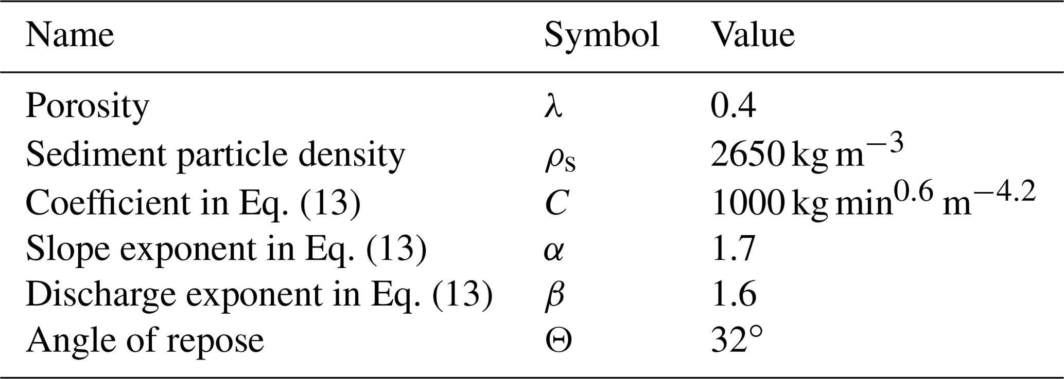
For the purpose of this study, an ideal simulation target can be a high and active mountain range (such as the Andes and Himalaya) where orographic effects appear clearly. However, we considered the physical limit in the applicable peak altitude of the single-layer SB model. The peak altitude of the Olympic Mountains, USA, for which the SB model was evaluated in a previous study (Smith and Barstad, 2004), is about 2.4 km. Taking this as a reference, the tectonic uplift rate u=1 mm yr−1 is used for all simulations, which yields a peak elevation of about 1.7 km (in most simulations) with a maximum of 2.7 km. In this way, we sought a reasonable compromise between the need to generate a high mountain range and the model limitation. This uplift rate is imposed uniformly over the domain and constantly throughout the entire simulation duration of 5 Ma. The tectonic response to unloading patterns induced by spatial variations in precipitation is ignored. The other model parameter values are summarized in Table 1.
Most landscape evolution modeling studies adopt random perturbations to reproduce dendritic stream network formation. Randomness can be imposed in various media, such as the initial topography (e.g., Han et al., 2015) and surface material (e.g., Paik and Kumar, 2008). We adopted the former approach, and the random noise, following a uniform distribution (not spatially auto-correlated), is given in the initial topography. The initial topography is nearly flat with a very mild slope () imposed to make sure surface water flows towards the ocean. The given random perturbation ( m) is tiny enough relative to the given initial elevation gap between two nearby cells (10−2 m), and so no depression zone forms in the initial topography. We implemented simulations initiated with the common setting described above but with varying model complexities. Two classes of simulations, namely “no feedback” and “co-evolution”, are presented below.
3.1 No-feedback simulations
No-feedback simulation results are obtained by running the LEGS model with spatially uniform rainfall, invariant over time. In no-feedback simulations, we focus on the effect of different rainfall excess rates P on long-term topography evolution. In the SB model, this can be seen as varying Po in Eq. (6) with zero wind velocity, which will negate the orographic effect (i.e., P=Po). We applied three scenarios of P=50, 100, and 150 mm d−1. We assumed these storms continue for 4 d (D=4); hence, the total rainfall depth for each event is 200, 400, and 600 mm, respectively. Each event is considered to correspond to a dominant storm occurring every 2 years (Δt1=2 years). With this Δt1, 5 Ma simulation time is discretized into 2.5 million time steps. Actual numerical simulations are implemented at daily resolution, i.e., four iterations per every Δt1. Hence, the computational load is 10 million iterations for 5 Ma simulation time in each scenario.
As the constant uplift is continuously imposed, the topographic relief increases over time in all cases, starting from zero (the sea level), and approaches a quasi-steady state (Fig. 1a). In this paper, the topographic relief or briefly relief refers to the gap between the peak elevation in the domain and the base level (which is zero as it refers to the sea level). As the greater P is imposed, the topography converges to the lower relief. This agrees with results from the earlier experimental study of Bonnet and Crave (2003).
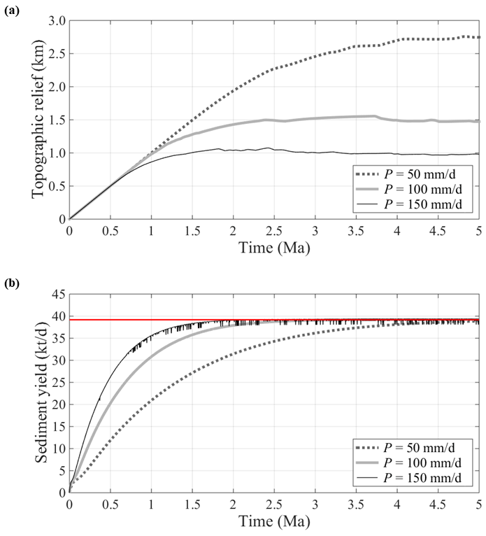
Figure 1Results of no-feedback simulations. Time variations of (a) the topographic relief and (b) the sediment yield from the entire domain are shown.
The sediment yield rapidly increases along with the topographic relief during the early stage of evolution (Fig. 1b). Rapid stream network formation at the early stage (Paik and Kumar, 2008) accelerates the sediment yield. As simulations proceed, the sediment yield converges to the rate of tectonic mass increase by the uplift (shown as a red horizon in Fig. 1b), regardless of P. This implies that the steady-state sediment yield is determined by the tectonic uplift rate, not rainfall. In contrast to the clear convergence of sediment yield (Fig. 1b), the convergence of relief is unclear as it exhibits continuous minor variations, after rapid early growth (Fig. 1a). This implies that our simulations produce quasi-steady, instead of purely steady, landscapes. The strict definition of the steady-state landscape requires no cell in the domain to show any elevation change over time. Referring to Eq. (14), this can be achieved if “the erosion rate is areally uniform and balances the rate of tectonic uplift” (Howard, 1994).
The balancing condition between the sediment yield and the uplift rate at the quasi-steady state helps explain distinct levels of quasi-steady reliefs with different P (Fig. 1a). To generate the same sediment yield at steady states, a high rainfall excess scenario is expected to pair with a low relief, as the sediment flux is given as the product of the runoff and gradient (Eq. 13). This argument is also in accordance with an earlier study about the detachment-limited condition (Whipple and Tucker, 1999). Note that the inverse relationship between the imposed P and the resultant relief is found to be nonlinear (as P linearly grows from 50 to 100 and 150 mm d−1, relief reduces nonlinearly, approximately from 2.7 to 1.5 and 1 km). This is due to the nonlinearity in Eq. (13).
One may notice that, in the scenario of the greatest rainfall (P=150 mm d−1), the sediment yield trend exhibits sharp fluctuations over time (Fig. 1b). The major mechanism causing these fluctuations is the formation and filling of depression zones. There is no depression zone initially, but they may appear during simulations as a result of over-erosion. Once formed, it only receives sediment inputs and generates no sediment output, and so the sediment yield from the domain drops. As a depression zone is filled with sediments, it disappears over time (Temme et al., 2006). To reduce over-erosion and depression zone formation, it would be needed to limit P and so ξ or to improve the time resolution, adopting a smaller Δt2. Enhancing resolution will further increase the already large number of iterations or computational load. Here, we found that Δt2=1 d is the resolution sufficiently fine to preclude over-erosion in all scenarios except the highest P(=150 mm d−1) scenario. Orographic rainfall generated in our co-evolution simulations (to be shown below) is less than P=150 mm d−1 as well, except some locally concentrated areas. Hence, we adopt Δt2=1 d throughout this study to save the computational load. Note that episodic landslides along coastlines can lead to sudden increase in sediment yield, although these events are undetected in our simulations.
3.2 Co-evolution simulations
We evaluated the long-term consequences of considering the orographic rainfall effect by coupling the LEGS and SB models. In co-evolution simulations, the rainfall field spontaneously evolves over time and space. We followed basic simulation settings of no-feedback simulations: dominant storm events lasting for 4 d (D=4, Δt2=1 d), considered per every 2 years (Δt1=2 years), and uniform tectonic uplift rate u=1 mm yr−1 imposed continuously for the entire simulation time of 5 Ma.
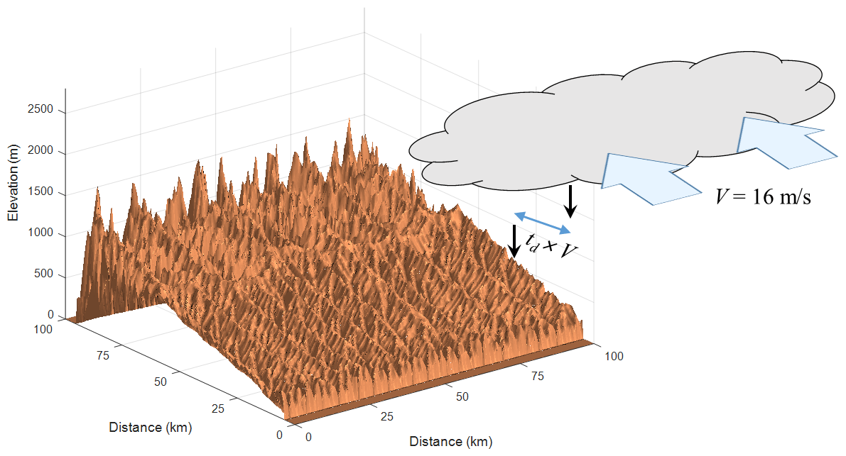
A number of simulation sets were designed with various atmospheric conditions. We evaluated the combined effects of the wind v, the delay times (tc and tf), and the temperature T on the rain field generation and long-term topography (Fig. 2). The wind direction is considered consistently north, i.e., U=0. As such, and a wide range of V were applied. Delay times are dependent on T. Anders et al. (2008) reported that (in seconds) is inversely related to T (in Kelvin), which can be approximated as
According to Eq. (16), three pairs of td and T are chosen for simulations: (1) td=600 s, T=287 K; (2) td=1200 s, T=284 K; and (3) td=1800 s, T=281 K. It has been known that the relative contribution of tc or tf in td is insignificant for the generation of orographic rainfall (Smith and Evans, 2007). Therefore, we simply set . For each pair, three levels of wind speed (V=8, 16, 24 m s−1) were tested, yielding nine scenarios in total. We imposed the base level rainfall Po=20 mm d−1 in Eq. (6). Each of these nine scenarios is considered a dominant storm.
Finally, the environmental lapse rate γ was carefully chosen to consider the physical limitation of the SB model. With T, γ determines the moist layer height (Eq. 8). Because no vertical variability is allowed in the SB model, applying the SB model to a topography higher than the moist layer is questionable. As described earlier, the maximum topographic height within which the SB model has been applied is 2.4 km. Considering this, we set γ=−6.3 K km−1, so that the range of the moist layer depth among nine scenarios is between 2.32 and 2.44 km. The moist adiabatic lapse rate Γm in Eq. (4) is given as −6.5 K km−1 in our theoretical simulations, referring to examples of Smith and Barstad (2004).
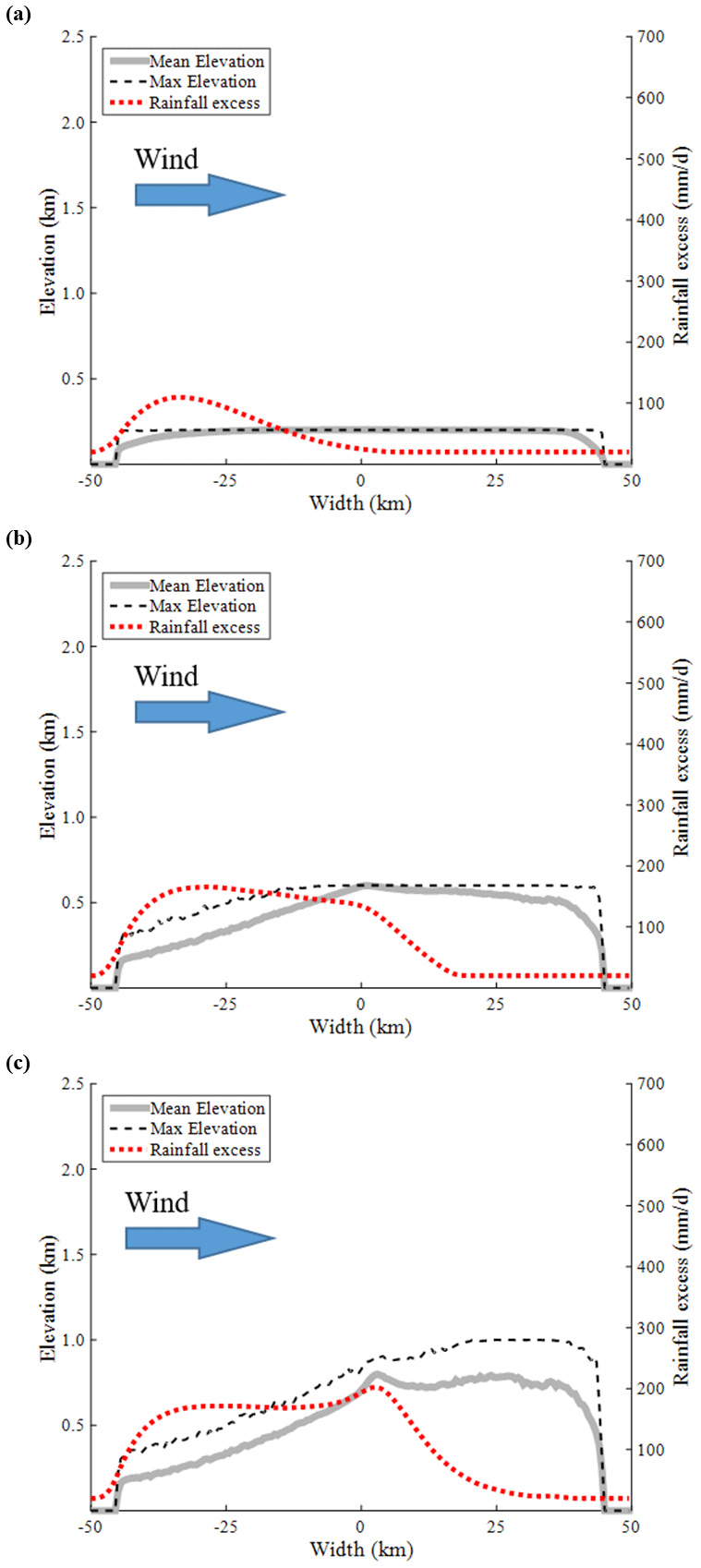
Topography evolves in a dramatically different manner between no-feedback and co-evolution simulations, implying significant topography–climate feedbacks. For example, two simulations of “no feedback” with P=100 mm d−1 and “co-evolution” with V=16 m s−1 and td=1200 s are compared in Fig. 3. These are chosen in that rainfall depths accumulated over the total simulation period are similar. Transects from no-feedback simulations are symmetric, whereas co-evolution simulations result in asymmetric transects. Co-evolution simulations resulted in the peak being pushed toward the lee side. Such peak migration matches the postulation of Smith (2006), the physical experiments of Bonnet (2009), and earlier simulation studies with the detachment-limited condition (Anders et al., 2008; Han et al., 2015). This will be further discussed in the next section. The formation of asymmetric transects is directly related to the asymmetric rainfall distribution (Willett, 1999). The SB model generates the rainfall as a function of wind vector, local topographic gradient, delay times, temperature, and other meteorological variables. Accordingly, the rain fields generated here differ from those from simpler models which assume rainfall as a monotonic function of elevation; the generated rainfall exhibits sharp increase from the northern coast, where the moist air first confronts the slope, and then gradual reduction as the moist air penetrates deeper inland (Fig. 3b).
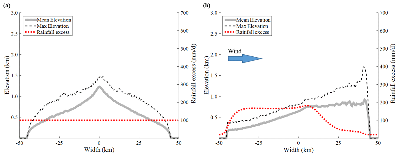
Figure 3North–south transects of landscapes and rainfall fields after 5 Ma simulation times. Results from (a) no-feedback (P=100 mm d−1) and (b) co-evolution (V=16 m s−1, td=1200 s, ) simulations are shown.
4.1 Asymmetry and relief in evolving topography
The formation of asymmetric topography is related to the time evolution of the rain field. On the initial flat surface, rainfall is given uniformly as Po without any orographic effect. Channel incision initiates at coasts (outlets) and then migrates upstream. This process should occur symmetrically across the initial transect. As the topography uplifts, the uniformity in the generated rain field is broken and the rain field evolves in an asymmetric fashion (Fig. 4a). The windward side receives more rainfall and so more runoff as well as sediment yield than the lee side. As a result, the channels on the windward side propagate upstream at a faster rate compared to those on the lee side (Fig. 4b). This leads to the downward peak migration and a steeper slope on the lee side (Fig. 4c).
As described above, the landscape experiences asymmetric erosion between the two sides (Fig. 5). On the other hand, the tectonic uplift is kept spatially uniform. Topography at each time step is determined through the trade-off between asymmetric erosion and uniform uplift. An interesting outcome of this complex adjustment is the development of the distinct peaks, which can be shown as a high ridge-valley relief at the lee side (Fig. 6a). These sharp peaks have been created by the interference between different evolutionary processes on the windward and lee sides. Whereas the windward side experiences high erosion due to enhanced rainfall during the evolution, many peaks remain intact on the lee side due to much less rainfall while being elevated (Fig. 4b). This results in a sharp contrast in elevation along the ridge line (Fig. 6a). Therefore, such features are a remnant of paleo-topography, similar to the monadnock.

Figure 5Time variation of sediment yield from co-evolution simulation. Simulation is implemented with V=16 m s−1 and td=1200 s. Red horizontal line corresponds to the mass balance with the tectonic uplift rate.
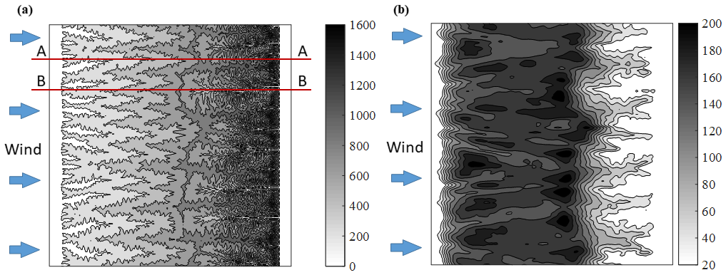
Figure 6Contour map of simulated (a) surface topography and (b) rainfall field from the co-evolution simulation with V=16 m s−1 and td=1200 s after 5 Ma (its transect shown in Fig. 3b). Numbers in the legend indicate the surface elevation (m) and rainfall excess rate (mm d−1), respectively.
Catchments on windward and lee sides develop alternately (Fig. 6a). For a large catchment developed on the windward side, its channel head deeply penetrates beyond the domain center and toward the lee side (e.g., cross section A–A in Fig. 6a). The space between upper areas of two adjacent catchments from the windward side is taken as a niche where a major lee-side catchment develops. Along the valley line of a major catchment on the lee side (e.g., cross section B–B in Fig. 6a), the head of the lee-side channel reaches close to the domain center. Through the topographic feedback on the local climate, generated rainfall also exhibits alternate spatial pattern (Fig. 6b).
In their study with the detachment-limited condition, Roe et al. (2002) claimed that the orographic rainfall reduces relief. In their model, rainfall increases monotonically with elevation and reaches a maximum at the peak elevation, which leads to a large peak incision and hence lower relief. However, the real rainfall pattern induced by the orographic effect is often far from such monotonic increase with elevation (e.g., Bookhagen and Burbank, 2006). The SB model generates the rainfall distribution much more complexly and diversely, in comparison with Roe et al. (2002). As a result, our simulations generate relief comparable to, or even greater (higher peak elevation) than, the relief obtained from no-feedback simulations for similar accumulated rainfall depths (e.g., Fig. 3). Depending on local atmospheric and topographic conditions, rainfall concentrates on different altitudes, influencing relief in different ways.
4.2 Roles of wind speed and total delay time in co-evolution
In the co-evolution modeling, the domain-averaged rainfall amount increases over time from the initial rate of Po (Fig. 7a and b). Such increase is in accordance with the relief growth and consequent feedback on rainfall. As shown in Eq. (3), the wind speed together with the topographic gradient is the primary factor that controls the rainfall. Essentially all rainfall depth generated beyond Po is due to the orographic effect (Eq. 6), which becomes activated only if a moist air parcel is pushed by wind and climbs uphill. Clearly, orographic rainfall shall be nil when V=0, and the generated rainfall amount tends to increase as a greater wind speed is imposed (Fig. 7a).
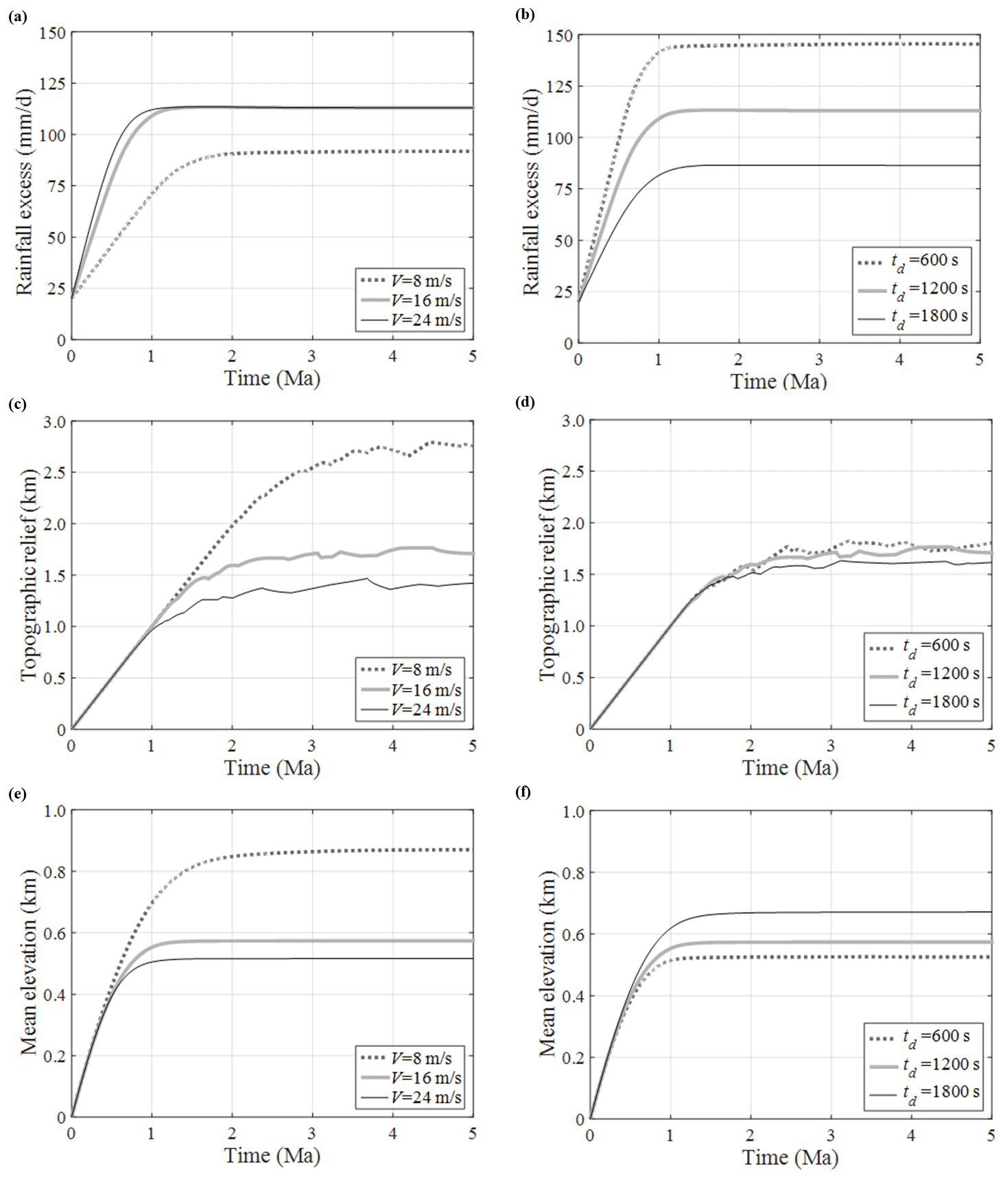
Figure 7Variations of (a, b) domain-averaged rainfall excess, (c, d) topographic relief, and (e, f) mean elevation during co-evolution simulations with different (a, c, e) V (td fixed as 1200 s) or (b, d, f) td (V fixed as 16 m s−1).
For a greater wind speed V, rainfall increases at a faster rate and converges to a greater amount. Such a relationship between V and P, though, was found to be nonlinear. A physical upper limit appears to exist as V greater than a certain value contributes no further increase in P. With td=1200 s and T=284 K, V=16 m s−1 seems to be the limit (Fig. 7a), although a greater rainfall is possible with a smaller td and warmer weather. The generation of P depends on both climatic (v) and topographic (∇z) factors (Eq. 3). Hence, to understand this nonlinear relationship and the limit in P, we need to understand the long-term effect of V on topography through rainfall and the topographic feedback on P, which is discussed below.
The resulting relief tends to be lower with a greater V (Fig. 7c). A similar tendency can be claimed for the mean elevation (Fig. 7e). These can be explained with the same reasoning described for no-feedback simulations (Fig. 1); i.e., greater wind speed is associated with more rainfall, and so it must be paired with a lower gradient to yield a sediment flux matching the mass generated at the imposed uplift rate. Interestingly, those two runs with V=16 and 24 m s−1, while producing similar domain-average rainfall (Fig. 7a), show a relief difference (Fig. 7c). This can be explained by another mechanism: a greater wind speed carries rainfall further uphill, toward the lee side (compare Figs. 3b and 8a). This results in a greater erosion over the peak, which also contributes to lower relief.
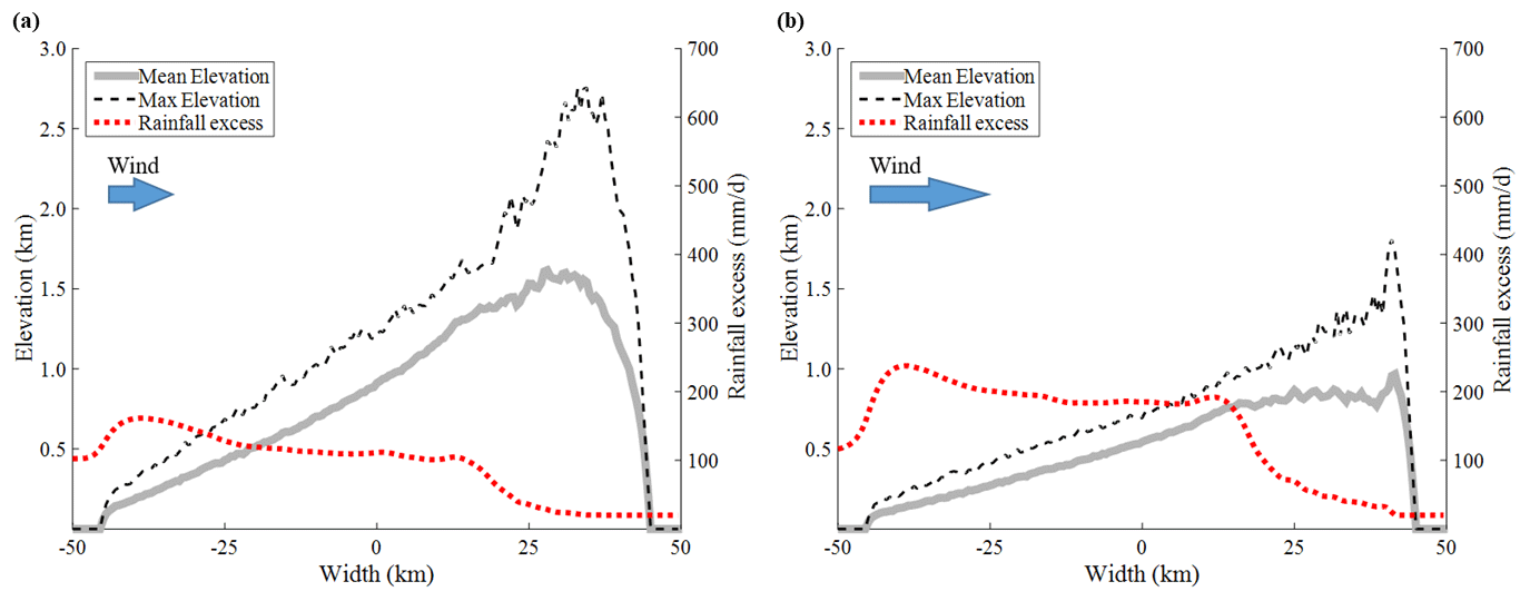
Figure 8Transects of landscapes and rainfall fields from co-evolution simulations after 5 Ma simulation times. Simulation settings are (a) V=8 m s−1, td=1200 s and (b) V=16 m s−1, td=600 s.
Despite the overall positive correlation between V and P (Fig. 7a), growing wind speed may act negatively on P. As discussed, with increasing V the relief tends to decrease. This gives a negative feedback on P. Hence, as V grows, there is a trade-off between the direct positive feedback on P and indirect (via a smaller relief) negative feedback on P. In two cases of V=16 and 24 m s−1 shown in Fig. 7a, these effects have coincidently become identical. In detail, the run with V=24 m s−1 has a greater positive feedback on P compared to the run with V=16 m s−1. However, this advantage is fully compensated by its greater negative feedback on P due to the lower relief, resulting in the same P.
In contrast to the V versus P relationship, P decreases as td grows (Fig. 7b). This is because a part of hydrometeors generated within the domain falls out of the domain in proportion to td. For example, the scenario with V=24 m s−1 and td=1800 s embeds 43 km horizontal displacement between locations of hydrometeor formation and rainfall (Fig. 2). Because a shorter delay time is related to a greater rainfall, one may also expect a robust relationship between td and the steady-state relief. Indeed, the robust relationship was found between td and the mean elevation (Fig. 7f). However, a similar relationship was not consistently obtained between td and relief (Fig. 7d). Although we find the inverse relationship between td and the rainfall amount (domain averaged) (Fig. 7b), a high rainfall induced by a short td concentrates downhill (compare Figs. 3b and 8b), which gives little effect on the peak elevation. Hence, no general relationship between td and relief can be established.
As discussed, both wind and td play primary roles in rain field generation. In fact, the combined effect of and td, rather than their individual effects, controls the co-evolutionary system. In this regard, the non-dimensional delay time t* (Eq. 1) was claimed as an important measure in shaping the resultant topography (Anders et al., 2008). However, our co-evolution modeling shows that steady-state topography can substantially differ even for an identical t*. For example, Fig. 8 illustrates two simulations with the same t* of 0.213 but very different resultant topography. The dramatic difference is due to multiple effects of V and td. While they give a similar effect on the horizontal displacement of rainfall, they act oppositely in producing overall rainfall amount: increased V mostly induces greater rainfall (domain average), whereas increased td reduces rainfall (Fig. 7).
As described previously, the pure steady state can be claimed if every cell in the domain exhibits no elevation change over time. This would be referred to as the dynamic equilibrium. In a macro perspective, the dynamic equilibrium can be inferred when the relief becomes steady (Hack, 1960; Willgoose, 1994). In co-evolution simulations, generated rainfall amount converges to a constant, which was claimed as another indicator of a steady state (Han et al., 2015). In our simulations, the rainfall (Fig. 7a and b), relief (Fig. 7c and d), mean elevation (Fig. 7e and f), and sediment yield (Fig. 5) all exhibit converging tendency, implying that any of these can be a potential indicator of the dynamic equilibrium. However, the convergence times all differ among these criteria. Further, the relief shows no strict convergence but continuous minor variations. These imply that the pure steady states have not been achieved.
4.3 Profile concavity
Along a natural stream, the local slope and drainage area A are associated as (Flint, 1974)
where θ is the concavity index. For alluvial channels, θ is mostly found to be positive (Howard, 1980; Tucker and Whipple, 2002; Byun and Paik, 2017), which indicates a concave profile. No-feedback simulations have well-reproduced concave profiles (e.g., Willgoose et al., 1991b; Willgoose, 1994; Paik, 2012). Here, a basic question is raised about the role of orographic rainfall in the profile formation. Roe et al. (2002) reported the impact of orographic rainfall on channel concavity in the 1D context. Below, we discuss the formation of channel profiles in a more general 3D landscape context.
Channel profiles at quasi-steady states, simulated from our co-evolutionary model, are mostly concave. Interestingly, we found that the profile concavity on the windward side becomes lower as V or td increases (Fig. 9). We can explain such variation with the scaling relationship below (Willgoose et al., 1991b):
In Eq. (18), ϕ is the exponent of the power-law relationship between the streamflow Q and drainage area A, i.e., Q∝Aϕ. A more comprehensive equation, considering the hydraulic geometry (Leopold and Maddock, 1953), Hack's law (Hack, 1957), and downstream fining (Brush, 1961) relationships, was derived by Byun and Paik (2017). Here, we use a briefer Eq. (18) for a simpler explanation. With fixed sediment transport parameters α and β (used in Eq. 13), Eq. (18) implies that the concavity θ is proportional to ϕ. Considering that the flow within a catchment propagates through a stream network downstream, if rainfall concentrates downstream, high ϕ is expected (significant downstream increase in streamflow). As V or td increases, the rainfall distribution moves upstream, which will result in a lower ϕ. From Eq. (18), hence, a greater V or td can lead to a decreased concavity. If ϕ is excessively low (and hence ϕβ<1), even a convex profile may form.
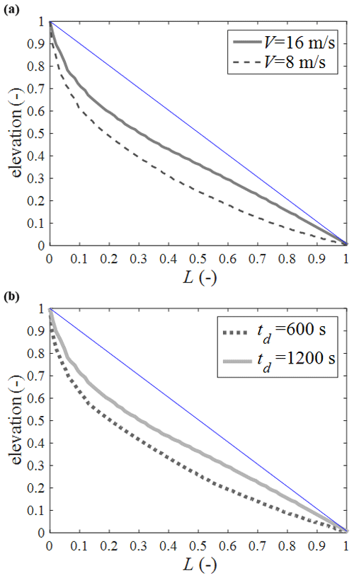
Figure 9Channel profiles after 5 Ma from simulations with (a) different V (td=1200 s) and (b) different td (V=16 m s−1). The profile of the main channel of the largest catchment in each simulation is shown. For comparison, profiles are normalized with maximum elevation and lengths. Blue straight line is drawn to help visually identify the profile concavity.
4.4 Limitations
It is important to note the limitations of the SB model in reproducing complex rainfall patterns in mountainous terrain. A critical weakness, relevant to our modeling approach, is that the SB model considers only single values of T and V (i.e., spatially uniform) for the entire domain. Ideally, a 2D gridded or even 3D weather model can be coupled with the surface process model. However, running such a model for a geologic timescale currently faces a computational challenge (we ran 10 million iterations for each scenario).
We have demonstrated that generated rainfall decreases as the delay time grows (Fig. 7b). This accounts for missing hydrometeors generated inside but falling out of the domain. However, there are also hydrometeors formed out of the domain and blown into the domain. Such an amount is yet to be counted for more realistic simulations. To count such an effect, we need to deeply investigate to what spatial extent such an effect shall be considered.
The scope of the present study is the bare soil landscape. In reality, vegetation has played a significant role in shaping the Earth's terrestrial surface. Incorporating vegetation dynamics could make co-evolution results much more complicated, as their feedback mechanisms have a complex link with water, solar radiation, nutrient, carbon, sediment (soil), topography, etc. Modeling vegetation dynamics in the whole landscape context has gradually progressed in the last decade (e.g., McGrath et al., 2012; Yetemen et al., 2015). These efforts promise that vegetation dynamics can be eventually incorporated into the proposed co-evolution framework.
Finally, we face a basic question on whether simulation results are testable. Documented co-evolution records are absolutely lacking. While this is a fundamental issue in the surface process modeling community, we need cooperative efforts to address it. We indeed witness new lights such as thermochronology in topography reconstruction and paleo-climate simulations using general circulation models.
As the close linkage between topography and climate has been acknowledged, numerical modeling of their co-evolution has become an important subject. In this study, a sophisticated numerical model is developed for the given purpose, and results from “no-feedback” and “co-evolution” simulations are compared. Detailed simulation results provide insights into the feedbacks and controls in co-evolution. Major scientific contributions from our theoretical study can be summarized below.
-
Evolving topography carries climatic and geomorphic footprints as shown in asymmetric transects and high valley relief on the lee side. Orographic rainfall affects resulting topographic relief in complex ways as spatial rainfall distribution greatly varies with meteorological conditions.
-
Evolved topography under the same non-dimensional delay time t* can significantly differ because of different roles of the wind speed and total delay time.
-
Concavity in the channel profile on the windward side becomes lower as the wind speed or delay time increases. This is explained with the known scaling relationship between the streamflow and upslope area, which is associated with the spatial rainfall distribution, driven by wind and topographic gradients.
In most landscape evolution modeling studies, rainfall has been considered as an input. On the basis of results shown in the present study, we suggest that the modeling community reconsider this practice: we should incorporate local climate dynamics into landscape evolution. Probably, this is the time to revise the terminology of the whole landscape evolution modeling as modeling of the evolution of the topography–climate coupled system. It is desired to further explore the roles of model (particularly meteorological) parameters and their combinations. In this sense, simulation results presented here are examples calling for future research needs in co-evolution modeling.
The sediment transport equation (Eq. 13) adopted in this study follows the classical formula, widely applied over a century. The first literature on this functional form traces back to du Boys (1879), whose sediment transport equation follows
where τb is the bed shear stress and τc is to encounter the initiation of motion (similar to but not exactly the same as the critical shear stress).
The bed shear stress can be estimated as , where ρ is the density of the fluid and H is the flow depth. In analogy, we can suggest , where Hc is the threshold depth corresponding to the initiation of the motion for the given slope . Substituting these into Eq. (A1) gives
If we take the Chezy formula, . Similarly, , where qc is the threshold value of q corresponding to Hc and τc. Then, Eq. (A2) can be rewritten as
Instead of Chezy, the Manning formula can also be used, i.e., and . Substituting these into Eq. (A2) gives
Equation (A2) states qs as a function of H. By transforming Eq. (A2) into Eq. (A3) or Eq. (A4), qs is expressed as a function of q. This is practically advantageous in that the evaluation of flow discharge is easier than the flow depth, particularly in the context of landscape evolution modeling.
Austrian engineer Schoklitsch implemented laboratory experiments to evaluate this type of equations with the grain size between 1 and 2 mm. The equation of Schoklitsch (1934) published in 1934 (introduced in English by Shulits, 1935) is
where qo is the threshold value of q for the initiation of motion and d is the grain size. The coefficient Co has a complex dimension. In English units (qs in lb s−1 ft−1, d in inches, q in ft3 s−1 ft−1), Co=86.7 lb in0.5 ft−3 was suggested from flume experiments (see Shulits, 1935), which is about 7000 kg mm0.5 m−3 in metric units (qs in kg s−1 m−1, d in millimeters, q in m3 s−1 m−1).
The above Eqs. (A3)–(A5), if the threshold term is neglected, commonly express the sediment transport rate for non-cohesive bed streams as the function of local slope and flow discharge, suggesting the form of Eq. (13). Quantifying the initiation of motion (the threshold term) is difficult, especially for small grains such as sands (Byun and Paik, 2017). Movement of sand particles has been observed even at very weak flow in flume experiments (e.g., Shvidchenko and Pender, 2000). Considering such a large uncertainty associated with it, the threshold term is often neglected when applying these equations to the scale of landscape evolution (Willgoose et al., 1991a; Tucker and Slingerland, 1994; Dietrich et al., 2003).
Other sediment transport equations such as Shields, Einstein–Brown, and Kalinske can also be expressed in the form of Eq. (13) (Raudkivi, 1967). Taking the Chezy or Manning formula, the Shields equation can be expressed as
Derivation from the Einstein–Brown equation is given in Henderson (1966) and later by Willgoose et al. (1991a) in more detail as
As shown in this Appendix, Eq. (13) can be derived from many existing sediment transport formulae. It has also been directly supported by flume experiments. While all these approaches result in the form of Eq. (13), they differ in the values of exponents α and β. For example, on the basis of Eq. (A3), , while Eq. (A4) implies α=1.4 and β=1.2. Even greater values are shown in Eq. (A6) or Eq. (A7). Another experimental study by MacDougall (1933) is also noteworthy, where the same functional form of Eq. (13) was suggested with a range of α between 1.25 and 2, while β is kept as unity. From the literature reviewed above, we can see that the ranges of α and β are and . Details of these ranges have been studied by Prosser and Rustomji (2000). Comparing Eqs. (13) and (A5), the coefficient C in Eq. (13) is interpreted as given α=1.5 and β=1. As α and β vary, the value and dimension of C in Eq. (13) are subject to variation.
The coupled simulation model LEGS used for the examples given in this paper is freely available for non-commercial purposes. Contact the corresponding author.
KP acquired funding, designed simulations, analyzed results, extracted scientific implications, and wrote the manuscripts. Through his Master's thesis, WK proposed to couple the SB and LEGS models and tested the early ideas about co-evolution. KP and WK developed the model code.
The authors declare that they have no conflict of interest.
This work was supported by a National Research Foundation of Korea (NRF) grant funded by the Korea government (MSIT) (no. 2018R1A2B2005772).
This paper was edited by Mariano Moreno de las Heras and reviewed by Arnaud Temme, Omer Yetemen, and one anonymous referee.
Anders, A. M., Roe, G. H., Montgomery, D. R., and Hallet, B.: Influence of precipitation phase on the form of mountain ranges, Geology, 36, 479–482, 2008. a, b, c, d, e, f, g, h
Archibald, E. D.: An account of some preliminary experiments with Biram's anemometers attached to kite strings or wires, Nature, 31, 66–68, https://doi.org/10.1038/031066a0, 1884. a
Barros, A. P. and Lettenmaier, D. P.: Dynamic modeling of orographically induced precipitation, Rev. Geophys., 32, 265–284, https://doi.org/10.1029/94RG00625, 1994. a
Barstad, I. and Smith, R. B.: Evaluation of an orographic precipitation model, J. Hydrometeorol., 6, 85–99, 2005. a
Bonnet, S.: Shrinking and splitting of drainage basins in orogenic landscapes from the migration of the main drainage divide, Nat. Geosci., 2, 897–897, https://doi.org/10.1038/Ngeo700, 2009. a
Bonnet, S. and Crave, A.: Landscape response to climate change: Insights from experimental modeling and implications for tectonic versus climatic uplift of topography, Geology, 31, 123–126, 2003. a
Bookhagen, B. and Burbank, D. W.: Topography, relief, and TRMM-derived rainfall variations along the Himalaya, Geophys. Res. Lett., 33, L08405, https://doi.org/10.1029/2006GL026037, 2006. a, b
Bookhagen, B. and Strecker, M. R.: Spatiotemporal trends in erosion rates across a pronounced rainfall gradient: Examples from the southern Central Andes, Earth Planet. Sc. Lett., 327, 97–110, https://doi.org/10.1016/j.epsl.2012.02.005, 2012. a
Braun, J. and Sambridge, M.: Modelling landscape evolution on geological time scales: A new method based on irregular spatial discretization, Basin Res., 9, 27–52, 1997. a, b
Brush Jr., L. M.: Drainage basins, channels, and flow characteristics of selected streams in central Pennsylvania, US Geological Survey Professional Paper 282-F, US Geological Survey, Washington, DC, 145–181, 1961. a
Byun, J. and Kim, J. W.: Development of a 2 dimensional numerical landscape evolution model on a geological time scale, J. Korean Geogr. Soc., 46, 673–692, 2011. a
Byun, J. and Paik, K.: Small profile concavity of a fine-bed alluvial channel, Geology, 45, 627, https://doi.org/10.1130/G38879.1, 2017. a, b, c
Champagnac, J.-D., Molnar, P., Sue, C., and Herman, F.: Tectonics, climate, and mountain topography, J. Geophys. Res., 117, B02403, https://doi.org/10.1029/2011JB008348, 2012. a
Chase, C. G.: Fluvial landsculpting and the fractal dimension of topography, Geomorphology, 5, 39–57, 1992. a
Colberg, J. S. and Anders, A. M.: Numerical modeling of spatially-variable precipitation and passive margin escarpment evolution, Geomorphology, 207, 203–212, 2014. a, b
Collier, C. G.: A representation of the effects of topography on surface rainfall within moving baroclinic disturbances, Q. J. Roy. Meteorol. Soc., 101, 407–422, 1975. a
Cooley, J. W. and Tukey, J. W.: An algorithm for the machine calculation of complex Fourier series, Math. Comput., 19, 297–301, https://doi.org/10.1090/S0025-5718-1965-0178586-1, 1965. a
Densmore, A. L., Ellis, M. A., and Anderson, R. S.: Landsliding and the evolution of normal-fault-bounded mountains, J. Geophys. Res., 103, 15203–15219, https://doi.org/10.1029/98JB00510, 1998. a
Dietrich, W. E., Bellugi, D. G., Sklar, L. S., Stock, J. D., Heimsath, A. M., and Roering, J. J.: Geomorphic transport laws for predicting landscape form and dynamics, in: Prediction in Geomorphology, edited by: Wilcock, P. R. and Iverson, R. M., American Geophysical Union, Washington, DC, https://doi.org/10.1029/135GM09, 2003. a
du Boys, M. P.: Le rhone et les rivières à lit affouillable, Annales des Ponts et Chaussées, 5, 141–195, 1879. a
Falvey, M. and Garreaud, R.: Wintertime precipitation episodes in central Chile: Associated meteorological conditions and orographic influences, J. Hydrometeorol., 8, 171–193, 2007. a
Ferrier, K. L., Huppert, K. L., and Perron, J. T.: Climatic control of bedrock river incision, Nature, 496, 206–209, https://doi.org/10.1038/nature11982, 2013. a
Flint, J. J.: Stream gradient as a function of order, magnitude, and discharge, Water Resour. Res., 10, 969–973, https://doi.org/10.1029/WR010i005p00969, 1974. a
Fraser, A. B., Easter, R. C., and Hobbs, P. V.: A theoretical study of the flow of air and fallout of solid precipitation over mountainous terrain: Part I. Airflow model, J. Atmos. Sci., 30, 801–812, 1973. a
Hack, J. T.: Studies of longitudinal stream profiles in Virginia and Maryland, US Geological Survey Professional Paper 294B, US Geological Survey, Washington, DC, 97 pp., 1957. a
Hack, J. T.: Interpretation of erosional topography in humid temperate regions, Am. J. Sci., 258-A, 80–97, 1960. a
Han, J., Gasparini, N. M., Johnson, J. P., and Murphy, B. P.: Modeling the influence of rainfall gradients on discharge, bedrock erodibility, and river profile evolution, with application to the Big Island, Hawai'i, J. Geophys. Res., 119, 1418–1440, https://doi.org/10.1002/2013JF002961, 2014. a
Han, J., Gasparini, N. M., and Johnson, J. P. L.: Measuring the imprint of orographic rainfall gradients on the morphology of steady-state numerical fluvial landscapes, Earth Surf. Proc. Land., 40, 1334–1350, https://doi.org/10.1002/esp.3723, 2015. a, b, c, d, e, f, g
Henderson, F. M.: Open Channel Flow, Macmillan, New York, 522 pp., 1966. a
Henderson-Sellers, B.: A new formula for latent heat of vaporization of water as a function of temperature, Q. J. Roy. Meteorol. Soc., 110, 1186–1190, https://doi.org/10.1002/qj.49711046626, 1984. a
Howard, A. D.: Thresholds in river regimes, in: Thresholds in Geomorphology, edited by: Coates, D. R. and Vitek, J. D., Allen and Unwin, Concord, Massachusetts, 227–258, 1980. a
Howard, A. D.: A detachment-limited model of drainage basin evolution, Water Resour. Res., 30, 2261–2285, 1994. a, b
Kim, W.: Influences of Climate and Tectonic Conditions on Long-Term Whole Landscape Evolution: Insights Obtained from Numerical Modeling Studies, MS Thesis, Korea University, Seoul, Korea, 2014. a
Knighton, A. D.: Fluvial Forms and Processes: A New Perspective, Arnold, London, 383 pp., 1998. a
Knuth, D. E.: Von Neumann's first computer program, in: Papers of John Von Neumann on Computing and Computer Theory, edited by: Aspray, W. and Burks, A., MIT Press, Cambridge, Massachusetts, 89–95, ISBN 978-0-262-22030-9, 1987. a
Leopold, L. B. and Maddock, T.: The hydraulic geometry of stream channels and some physiographic implications, US Geological Survey Professional Paper 252, US Geological Survey, Washington, DC, 57 pp., 1953. a
Leopold, L. B., Wolman, M. G., and Miller, J. P.: Fluvial Processes in Geomorphology, Freeman, San Francisco, 522 pp., 1964. a
MacDougall, C. H.: Bed‐Sediment transportation in open channels, Eos Trans. Am. Geophys. Union, 14, 491–495, https://doi.org/10.1029/TR014i001p00491, 1933. a
Masek, J. G., Isacks, B. L., Gubbels, T. L., and Fielding, E. J.: Erosion and tectonics at the margins of continental plateaus, J. Geophys. Res., 99, 13941–13956, https://doi.org/10.1029/94JB00461, 1994. a, b
McGrath, G. S., Paik, K., and Hinz, C.: Microtopography alters self-organized vegetation patterns in water-limited ecosystems, J. Geophys. Res., 117, G03021, https://doi.org/10.1029/2011JG001870, 2012. a
Molnar, P. and England, P.: Late Cenozoic uplift of mountain ranges and global climate change: Chicken or egg?, Nature, 346, 29–34, https://doi.org/10.1038/346029a0, 1990. a
Moon, S., Chamberlain, C. P., Blisniuk, K., Levine, N., Rood, D. H., and Hilley, G. E.: Climatic control of denudation in the deglaciated landscape of the Washington Cascades, Nat. Geosci., 4, 469–473, https://doi.org/10.1038/Ngeo1159, 2011. a
Norton, K. and Schlunegger, F.: Migrating deformation in the Central Andes from enhanced orographic rainfall, Nat. Commun., 2, 584, https://doi.org/10.1038/ncomms1590, 2011. a
Paik, K.: Global search algorithm for nondispersive flow path extraction, J. Geophys. Res., 113, F04001, https://doi.org/10.1029/2007JF000964, 2008. a
Paik, K.: Simulation of landscape evolution using global flow path search, Environ. Model. Softw., 33, 35–47, https://doi.org/10.1016/j.envsoft.2012.01.005, 2012. a, b
Paik, K. and Kumar, P.: Emergence of self‐similar tree network organization, Complexity, 13, 30–37, 2008. a, b
Park, J. I. and Singh, V. P.: Temporal and spatial characteristics of rainfall in the Nam river dam basin of Korea, Hydrol. Process., 10, 1155–1171, 1996. a
Pelletier, J. D.: The impact of snowmelt on the late Cenozoic landscape of the southern Rocky Mountains, USA, GSA Today, 19, 4–11, https://doi.org/10.1130/GSATG44A.1, 2009. a
Prosser, I. P. and Rustomji, P.: Sediment transport capacity relations for overland flow, Prog. Phys. Geogr., 24, 179–193, https://doi.org/10.1177/030913330002400202, 2000. a
Puvaneswaran, K. M. and Smithson, P. A.: Precipitation-elevation relationships over Sri Lanka, Theor. Appl. Climatol., 43, 113–122, 1991. a
Raudkivi, A. J.: Loose Boundary Hydraulics, Pergamon Press, Oxford, New York, 331 pp., 1967. a
Reiners, P. W., Ehlers, T. A., Mitchell, S. G., and Montgomery, D. R.: Coupled spatial variations in precipitation and long-term erosion rates across the Washington Cascades, Nature, 426, 645–647, https://doi.org/10.1038/nature02111, 2003. a
Roe, G. H., Montgomery, D. R., and Hallet, B.: Effects of orographic precipitation variations on the concavity of steady-state river profiles, Geology, 30, 143–146, 2002. a, b, c, d
Roe, G. H., Whipple, K. X., and Fletcher, J. K.: Feedbacks among climate, erosion, and tectonics in a critical wedge orogeny, Am. J. Sci., 308, 815–842, https://doi.org/10.2475/07.2008.01, 2008. a, b
Rossby, C.-G.: Thermodynamics applied to air mass analysis, M.I.T. Meteorology Paper 1, Massachusetts Institute of Technology, Cambridge, Massachusetts, 1932. a
Schoklitsch, A.: Der Geschiebetrieb und Die Geschiebefracht, Wasserkraft Wasserwirt., 39, 1–7, 1934. a
Shin, S. and Paik, K.: An improved method for single flow direction calculation in grid digital elevation models, Hydrol. Process., 31, 1650–1661, https://doi.org/10.1002/hyp.11135, 2017. a
Shulits, S.: The Schoklitsch bed-load formula, Engineering, 687, 644–646, 1935. a, b
Shvidchenko, A. B. and Pender, G.: Flume study of the effect of relative depth on the incipient motion of coarse uniform sediments, Water Resour. Res., 36, 619–628, https://doi.org/10.1029/1999WR900312, 2000. a
Smith, R. B.: The influence of mountains on the atmosphere, Adv. Geophys., 21, 87–230, 1979. a
Smith, R. B.: A linear upslope-time-delay model for orographic precipitation, J. Hydrol., 282, 2–9, 2003. a
Smith, R. B.: Progress on the theory of orographic precipitation, in: Tectonics, Climate, and Landscape Evolution, edited by: Willett, S. D., Hovius, N., Brandon, M. T., and Fisher, D. M., Geological Society of America Special Paper 398, Penrose Conference Series, Geological Society of America, Boulder, CO, 1–16, https://doi.org/10.1130/2006.2398(01), 2006. a
Smith, R. B. and Barstad, I.: A linear theory of orographic precipitation, J. Atmos. Sci., 61, 1377–1391, 2004. a, b, c, d, e, f
Smith, R. B. and Evans, J. P.: Orographic precipitation and water vapor fractionation over the southern Andes, J. Hydrometeorol., 8, 3–19, https://doi.org/10.1175/JHM555.1, 2007. a, b
Smith, T. R. and Bretherton, F. P.: Stability and the conservation of mass in drainage basin evolution, Water Resour. Res., 8, 1506–1529, https://doi.org/10.1029/WR008i006p01506, 1972. a
Temme, A. J. A. M., Schoorl, J. M., and Veldkamp, A.: Algorithm for dealing with depressions in dynamic landscape evolution models, Comput. Geosci., 32, 452–461, https://doi.org/10.1016/j.cageo.2005.08.001, 2006. a
Temme, A. J. A. M., Armitage, J., Attal, M., Gorp, W., Coulthard, T. J., and Schoorl, J. M.: Developing, choosing and using landscape evolution models to inform field-based landscape reconstruction studies, Earth Surf. Proc. Land., 42, 2167–2183, https://doi.org/10.1002/esp.4162, 2017. a, b
Tucker, G. E. and Slingerland, R. L.: Erosional dynamics, flexural isostasy, and long-lived escarpments: A numerical modeling study, J. Geophys. Res., 99, 12229–12243, https://doi.org/10.1029/94JB00320, 1994. a, b, c
Tucker, G. E. and Whipple, K. X.: Topographic outcomes predicted by stream erosion models: Sensitivity analysis and intermodel comparison, J. Geophys. Res., 107, 2179, https://doi.org/10.1029/2001JB000162, 2002. a
Tucker, G. E., Lancaster, S. T., Gasparini, N. M., Bras, R. L., and Rybarczyk, S. M.: An object-oriented framework for distributed hydrologic and geomorphic modeling using triangulated irregular networks, Comput. Geosci., 27, 959–973, https://doi.org/10.1016/S0098-3004(00)00134-5, 2001. a
Ward, D. J. and Galewsky, J.: Exploring landscape sensitivity to the Pacific Trade Wind Inversion on the subsiding island of Hawaii, J. Geophys. Res., 119, 2048–2069, https://doi.org/10.1002/2014JF003155, 2014. a
Whipple, K. X. and Tucker, G. E.: Dynamics of the stream-power river incision model: Implications for height limits of mountain ranges, landscape response timescales, and research needs, J. Geophys. Res., 104, 17661–17674, 1999. a
Willett, S. D.: Orogeny and orography: The effects of erosion on the structure of mountain belts, J. Geophys. Res., 104, 28957–28981, https://doi.org/10.1029/1999JB900248, 1999. a, b
Willgoose, G.: A physical explanation for an observed area-slope-elevation relationship for catchments with declining relief, Water Resour. Res., 30, 151–159, https://doi.org/10.1029/93WR01810, 1994. a, b
Willgoose, G., Bras, R. L., and Rodríguez-Iturbe, I.: A coupled channel network growth and hillslope evolution model: 1. Theory, Water Resour. Res., 27, 1671–1684, 1991a. a, b, c, d, e
Willgoose, G., Bras, R. L., and Rodríguez-Iturbe, I.: A physical explanation of an observed link area-slope relationship, Water Resour. Res., 27, 1697–1702, https://doi.org/10.1029/91WR00937, 1991b. a, b
Wobus, C. W., Tucker, G. E., and Anderson, R. S.: Does climate change create distinctive patterns of landscape incision?, J. Geophys. Res., 115, F04008, https://doi.org/10.1029/2009JF001562, 2010. a
Yetemen, O., Istanbulluoglu, E., Flores-Cervantes, J. H., Vivoni, E. R., and Bras, R. L.: Ecohydrologic role of solar radiation on landscape evolution, Water Resour. Res., 51, 1127–1157, https://doi.org/10.1002/2014WR016169, 2015. a
Zhang, Y., Slingerland, R., and Duffy, C.: Fully-coupled hydrologic processes for modeling landscape evolution, Environ. Model. Softw., 82, 89–107, https://doi.org/10.1016/j.envsoft.2016.04.014, 2016. a