the Creative Commons Attribution 4.0 License.
the Creative Commons Attribution 4.0 License.
 | 10 May 2021
Using data assimilation to optimize pedotransfer functions using field-scale in situ soil moisture observations
Eleanor Blyth
Hollie Cooper
Rich Ellis
Ewan Pinnington
Simon J. Dadson
Soil moisture predictions from land surface models are important in hydrological, ecological, and meteorological applications. In recent years, the availability of wide-area soil moisture measurements has increased, but few studies have combined model-based soil moisture predictions with in situ observations beyond the point scale. Here we show that we can markedly improve soil moisture estimates from the Joint UK Land Environment Simulator (JULES) land surface model using field-scale observations and data assimilation techniques. Rather than directly updating soil moisture estimates towards observed values, we optimize constants in the underlying pedotransfer functions, which relate soil texture to JULES soil physics parameters. In this way, we generate a single set of newly calibrated pedotransfer functions based on observations from a number of UK sites with different soil textures. We demonstrate that calibrating a pedotransfer function in this way improves the soil moisture predictions of a land surface model at 16 UK sites, leading to the potential for better flood, drought, and climate projections.
- Article
(1349 KB) - Full-text XML
- BibTeX
- EndNote


Soil moisture is an important physical variable, significant in agriculture (Pinnington et al., 2018), flood events (Koster et al., 2010; Berghuijs et al., 2019), and processes related to weather and climate (Seneviratne et al., 2010). Land surface models such as the Joint UK Land Environment Simulator (JULES) can be used to make predictions of soil moisture and generally rely on empirical pedotransfer functions (PTFs) to relate readily available or easy-to-measure soil characteristics such as soil texture to the soil hydraulics parameters required by the model (e.g. Van Looy et al., 2017)
There are a number of different types of pedotransfer function, as noted in Van Looy et al. (2017) and Hodnett and Tomasella (2002), with different inputs and outputs depending partly on the representation of soil physics processes of the chosen land surface model. In “class” approaches, soil types are clustered into groups, and hydraulic model parameters are then obtained from a lookup table (Wösten et al., 1999); this results in discrete soil hydraulics parameter sets. Alternatively, continuous pedotransfer functions take soil characteristic information from each sample of interest and apply the function to produce continuous soil hydraulics parameter sets (e.g. Cosby et al., 1984; Hodnett and Tomasella, 2002; Schaap et al., 2001).
To date, pedotransfer functions have been derived by fitting to results from field or laboratory experiments on point- or small-scale soil samples (centimetre to metre), despite the fact that land surface models are generally applied at larger (field to kilometre) scales. The recent development of novel in situ techniques for measuring soil moisture over field rather than point scale presents an opportunity to test whether land surface models, in conjunction with commonly used pedotransfer functions, are able to reproduce field-scale soil moisture observations.
In this paper, we have compared JULES soil moisture predictions with soil moisture observations from the COSMOS-UK dataset (Stanley et al., 2021); these observations are measured by cosmic ray neutron sensor (CRNS) instruments over a footprint of up to 120 000 m2. We have then used the LaVEnDAR four-dimensional ensemble variational data assimilation framework (Pinnington et al., 2020) to combine COSMOS-UK soil moisture observations at 16 sites with equivalent JULES soil moisture estimates. We have thereby optimized constants in the Cosby pedotransfer function (Cosby et al., 1984). This results in a newly calibrated set of pedotransfer functions based on field-scale soil moisture observations across 16 sites with a range of soil types. This approach allows us to test whether we can improve the performance of the model by optimizing the pedotransfer functions for larger scales using field-scale soil moisture observations. Our approach also allows for comparison of the soil hydraulics parameters generated using field-scale (∼ hundreds of metres) soil moisture measurements with those generated by the original pedotransfer functions, which are based on small-scale (∼ centimetres) measurements. We chose to optimize the pedotransfer functions rather than directly optimizing soil physics parameters since this preserves the physical relationships between soil physics parameters that the pedotransfer functions describe. This approach also has the advantage that we can assimilate observations from all sites simultaneously to produce one set of pedotransfer functions applicable at all 16 study sites. The same pedotransfer function could then potentially be applied anywhere in the UK that soil texture information is available.
We use CRNS soil moisture measurements in this study. Larger scale soil moisture measurements are also increasingly available from satellite products, and these have been used to good effect in data assimilation frameworks with land surface models (e.g. Pinnington et al., 2018; Liu et al., 2011; De Lannoy and Reichle, 2016; Yang et al., 2016). The advantage of the CRNS measurements used here is that they provide a more direct soil moisture measurement than those from satellites. CRNS soil measurements are also representative of depths of approximately 10 to 30 cm, compared to the top 5 to 10 cm for satellite retrievals.
An alternative approach to assimilate CRNS soil moisture measurements into land surface models is taken in Brunetti et al. (2019), Han et al. (2015), and Mwangi et al. (2020). These studies use neutron counts from CRNS instruments as observations, combined with the COSMIC method presented in Shuttleworth et al. (2013) to map modelled soil moisture estimates into equivalent neutron counts. In this study we instead directly compare modelled and CRNS-derived soil moisture.
The rest of the paper is organized as follows: in Sect. 2, we outline the JULES land surface model and the COSMOS-UK data used in this study; we also describe the data assimilation experiment we have performed and introduce the metric we deployed to measure how well the model fits the observations. In Sect. 3, we present results, showing that we can use COSMOS-UK observations from 2017 to improve the fit between the JULES model output and observations over 2 years at all the sites we included. We discuss our results in the context of changes in the JULES soil physics parameters in Sect. 4. In Sect. 5, we conclude that it is possible to optimize pedotransfer functions with field-scale soil moisture measurements and that this markedly improves the fit of JULES soil moisture estimates to COSMOS-UK observations.
2.1 JULES land surface model
JULES uses the Darcy–Richards equation to model soil hydraulic processes (Best et al., 2011), so that the downward water flux, W, between adjacent soil layers is given by
where Ψ is the soil matric suction, K is the soil hydraulic conductivity, and z is the distance from the soil surface in the vertical direction.
JULES provides two options for representing the relation between soil water content, θ, matric suction, and hydraulic conductivity; in this paper we use the Brooks and Corey soil physics option (Best et al., 2011; Brooks and Corey, 1964), where we assume
and
In Eqs. (2) and (3), θs, Ks, and Ψs are values of soil moisture, hydraulic conductivity, and soil matric suction at saturation; b is a soil-dependent constant with a value usually determined through a pedotransfer function. The soil physics parameters used in the implementation of Brooks and Corey soil physics in JULES are briefly described in Table 1; more details are available in Best et al. (2011) or in the JULES user guide (2020).

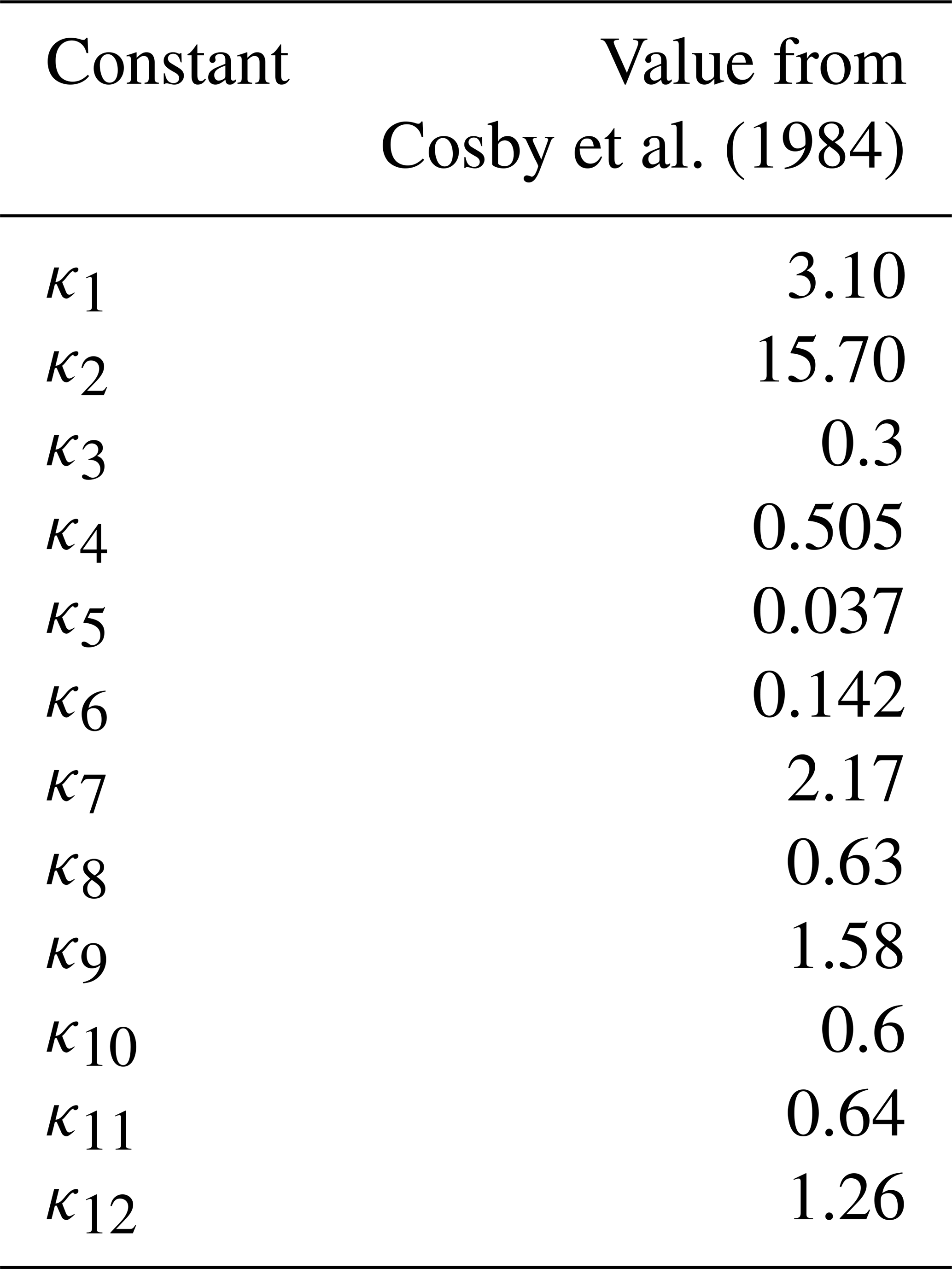
The values of the eight soil physics parameters outlined in Table 1 are generally calculated via a set of pedotransfer functions. Here we use the Cosby pedotransfer functions, which have the following mathematical formulation (Cosby et al., 1984; Marthews et al., 2014):
where fclay, fsand, and fsilt are fractions of clay, sand, and silt in the soil, by weight. Equations (8) and (9) are rearrangements of Eq. 2 at fixed values of matric suction corresponding to the wilting and critical points. Equation (10) is a linear combination of the assumed heat capacities of sand, silt, and clay, weighted by their relative fractions, and Eq. 11 is as given in Dharssi et al. (2009). The values of the constants κ1 to κ12 usually used in Eqs. (4) to (11) are those given in Cosby et al. (1984); we present them in Table 2. These values are empirically determined from 1448 small soil samples (centimetre dimensions) taken from 23 states in the United States (for further details of the soil samples and sampling methods, see Rawls, 1976, and Holtan, 1968). The values of the constants given here match those in Marthews et al. (2014) (with soil fraction multipliers adjusted for fraction, rather than percentage, of soil by weight).
Cosby et al. (1984)Table 2Values of the constants commonly used in the Cosby pedotransfer functions.
JULES requires meteorological driving data to produce soil moisture estimates. The required input variables are air pressure, air temperature, humidity, downward fluxes of shortwave and longwave radiation, precipitation, and wind speed. In this paper we have used half-hourly meteorological observations measured at COSMOS-UK sites as driving data; in this way we can use JULES to give soil moisture predictions at any COSMOS-UK sites with sufficiently complete meteorological data.
JULES provides estimates of soil moisture at various depths; in the standard configuration used here these correspond to four layers, with depths [0,10 cm], [10 to 35 cm], [35 to 100 cm], and [100 to 300 cm]. The JULES layers are often referred to by their thicknesses, which are 10, 25, 65, and 200 cm respectively. Here, we refer to the soil moisture estimates for the four layers as SM10, SM25, SM65, and SM200.
2.2 COSMOS-UK soil moisture data
The COSMOS-UK project comprises a network of soil moisture monitoring stations across the United Kingdom, providing long-term soil moisture measurements at around 50 sites. Data for 2013 to 2019 are available in the EIDC archive (Stanley et al., 2021). Soil moisture observations are made using an innovative cosmic ray neutron sensor (CRNS) instrument at each site; these provide a measurement of soil moisture over an area of up to 120 000 m2 (∼ 30 acres) (Antoniou et al., 2019; Evans et al., 2016). The CRNS at each site counts fast neutrons within the sensor's footprint. These counts are corrected for local meteorological conditions using in situ measurements and also background neutron intensity using data from a neutron monitoring station (Evans et al., 2016). The corrected counts are then calibrated for site-specific soil properties determined from destructive soil sampling conducted after site installation. Soil samples were collected from each site following Köhli et al. (2015) and were returned to UKCEH for laboratory analysis. The results were used to determine reference soil moisture, lattice and bound water, bulk density, and organic matter for the day of sampling and are subsequently used to derive soil water content from the corrected CRNS counts. The majority of sites explored in this study are grasslands, and it is therefore expected that CRNS soil moisture results are not significantly affected by seasonal changes in biomass (Baatz et al., 2014).
We have used daily averaged soil moisture data from 16 COSMOS-UK sites as observations in this paper. The sites were selected based on completeness of soil moisture and meteorological data over a 3-year period from 2016–2018 and are listed in Table 3, with details of land cover and broad soil descriptions taken from Antoniou et al. (2019). Locations of the sites are shown in Fig. 1. For more details of each of the sites, see Antoniou et al. (2019). The Cosby pedotransfer function was designed to work for mineral soils, and the CRNS calibration is most reliable at sites with minimal vegetation. We therefore consider that the first seven sites listed in Table 3 are those at which the JULES model can be expected to provide a good match to observations via our chosen PTF; soil types and land cover at the remaining sites mean that JULES may not be able to represent the observed soil moisture time series as accurately.
Table 3COSMOS-UK sites selected for this study. “Heath” indicates some shrubs are present at the site.
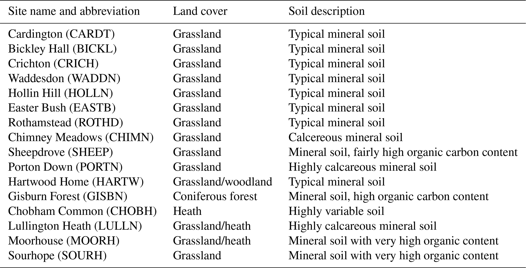

Figure 1Locations of COSMOS-UK sites used in this study.
Both the depth and the footprint over which the CRNS measures soil moisture change with soil moisture (Evans et al., 2016; Köhli et al., 2015; Antoniou et al., 2019), with the footprint and depth of the measurement both becoming smaller as soil moisture increases. The COSMOS-UK dataset (Stanley et al., 2021) includes estimates of the depth over which each daily soil moisture value is valid, known as a D86 value. Measurements of several other environmental variables are made at COSMOS-UK sites, using a suite of instrumentation. These include point soil moisture and temperature measurements at various depths in the soil and meteorological variables. We have used half-hourly in situ meteorological data from the COSMOS-UK dataset as driving data for the JULES model.
2.3 Data assimilation
Data assimilation is a group of methods in which information from models and observations is combined in order to give the best estimate of the state of a physical system and/or model parameter values. In this paper, we have used the four-dimensional ensemble variational data assimilation technique, LaVEnDAR, which is introduced in Pinnington et al. (2020) and is based on Liu et al. (2008). We use LaVEnDAR to optimize 12 constants, κ1 to κ12, in the Cosby pedotransfer functions (Eqs. 4 to 11) based on estimates of soil moisture from JULES and corresponding field-scale observations of soil moisture from COSMOS-UK. LaVEnDAR optimizes κ1 to κ12 here by minimizing a cost function with two terms. The first term is a measure of the difference between the observed and modelled soil moisture, and the second term is a measure of the difference between prior and posterior values of κ1 to κ12.
The values of κ1 to κ12 are assumed to be constant in time and space; the same values are used across all sites to generate soil JULES moisture estimates via the pedotransfer functions.
2.4 Experimental details
In order to use COSMOS-UK data with JULES outputs in the LaVEnDAR scheme, we require both sets of soil moisture values to correspond to the same soil depth. We have therefore devised a weighted depth approach, in which we extract from each JULES prediction an average soil moisture corresponding to the UK-COSMOS observed depth. The observed depth changes with soil moisture and with horizontal distance from the CRNS instrument; here we have used the reported observation depth at 75 m from the CRNS (in the horizontal direction). For each day, we calculate a depth-adjusted JULES soil moisture estimate, SMdepth, depending on the 75 m observation depth value, D86, provided for that day, such that
where SM10, SM25, and SM65 are the JULES-predicted soil moisture values from the [0,10 cm], [10 to 35 cm], and [35 to 100 cm] layers respectively, and the D86 value is given in centimetres. In this way, thickness-weighted contributions to the soil moisture are taken from every JULES layer which would be wholly or partly contained within the D86 depth. We have not taken the COSMOS-UK variable footprint into account in this study.
In this paper we have used an ensemble size of 50, as in related experiments in Pinnington et al. (2020) and Liu et al. (2008). In order to implement the LaVEnDAR scheme we conducted the following:
-
We generated a 50-member ensemble of each of the 12 PTF constants κ1 to κ12. These were obtained by sampling from a Gaussian distribution centred on the value given in Table 2, with standard deviation equal to 10 % of the mean. This standard deviation value was chosen fairly arbitrarily; future work could assess the sensitivity of the results to the values chosen for each PTF constant.
-
We assembled 50 unique sets of 12 constants κ1 to κ12.
-
We used each unique set of constants in Eqs. (4) to (11) to generate 50 sets of soil physics parameters for each site. Soil texture information for each site was taken from the Harmonized World Soil Database (HWSD) (Fischer et al., 2008).
-
We used the soil parameter sets to run 50 realizations of JULES at each of our selected sites over a 2-year time window to create a prior ensemble of 50 soil moisture time series per site.
-
We used the LaVEnDAR scheme to generate a new, posterior ensemble of values for each of the 12 PTF constants, taking into account COSMOS-UK soil moisture observations from 2017. Here, we assumed uncorrelated observation errors of 50 % of the mean soil moisture value at each site.
-
We used the new posterior ensemble of PTF constants to generate 50 posterior sets of soil physics variables at each site.
-
We ran 50 posterior realizations of JULES at each site to create posterior soil moisture time series.
These steps are also shown in schematic form in Fig. 2.
We assume that the soil texture values from the HWSD are correct; they are not changed during the data assimilation process. We used a global soil texture dataset since site-specific soil texture observations were not available; using a global soil texture dataset also has the advantage that our method then has the potential for extension to other UK areas without local soil measurements. Other open-source global soil texture products are also available, e.g. SoilGrids (Hengl et al., 2017). We acknowledge that there can be discrepancies between the HWSD and local measurements (e.g. Zhao et al., 2018), but our decision to use the HWSD here follows recent successful integration of soil texture data from the HWSD with JULES in studies such as Martínez-de la Torre et al. (2019), Ritchie et al. (2019), and Ehsan Bhuiyan et al. (2019).
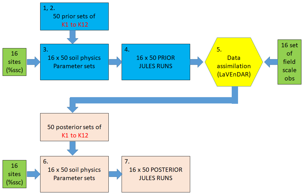
Figure 2Schematic showing data assimilation experimental design; % ssc refers to site-specific fractions of sand, silt, and clay in the soil. In this study, only observations from 2017 (at each site) were used in the assimilation algorithm.
We have assumed a high observation error value in this experiment. The daily soil moisture measurements we use are averaged from hourly soil moisture measurements; analysis of these data shows that the standard deviation of the hourly data around the daily mean is approximately 20 %. We have inflated this here to 50 % observation error; we note that similar observation error covariance inflation techniques have been used in, for example, assimilation of satellite observations in numerical weather prediction (Fowler et al., 2018; Hilton et al., 2009). The reason for inflating the observation error is essentially because we found that smaller observation error values impacted negatively on the posterior soil moisture results. We suggest that inflation of the observation error is necessary here to compensate for otherwise neglected sources of error (e.g. the error in converting neutron counts to soil moisture) and for the assumption of uncorrelated observation error; in fact there will likely be intra-site correlations between observation errors due to site-specific instrument calibration.
We have used COSMOS-UK measurements from 2017 only in our data assimilation experiments but compared the prior and posterior JULES runs from 2017 and 2018 with observations.

Figure 3Observed and modelled (ensemble mean) soil moisture time series at Bickley Hall (BICKL). The dotted line separates the period over which observations have been used for assimilation (2017) from the period in which no observations have been assimilated (2018).
2.5 Metrics
In order to assess how well our prior and posterior JULES runs match COSMOS-UK observations, we require a metric. Here we have used the Kling–Gupta efficiency metric, as described in Gupta et al. (2009) and Knoben et al. (2019), to compare the goodness of fit between observed and modelled (ensemble mean) soil moisture times series. The Kling–Gupta efficiency (KGE) is given by
where
and
In Eqs. (14) and (15), μmodel and μobs are mean values of the modelled and measured soil moisture time series respectively; σmodel and σobs are the standard deviations in the modelled and observed soil moisture time series. The value of r is the Pearson correlation coefficient between the model and the observation time series data and can vary between −1 (anti-correlation) and 1 (perfect correlation), with a score of 0 indicating no correlation. The value of α reflects how well the spread in the modelled soil moisture values matches that of the observations, with a value of 1 corresponding to perfect matching. Equation (15) shows that the value of β represents bias between the model and observations, with a value of 1 indicating zero bias. Since α and β can be larger or smaller than 1, the value of the KGE can range between 1 (perfect model fit to data) and very large negative values. In Knoben et al. (2019), the authors argue that while in some studies a threshold of KGE ≥ 0 has been used to denote “good” model performance, a lower threshold of KGE ≥ −0.41 is required for the model to perform better than a mean persistence forecast. We used Python 3.7.1 to calculate metrics and prepare plots.
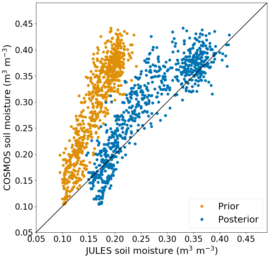
Figure 4Observed vs. modelled (ensemble mean) soil moisture at Bickley Hall (BICKL) for prior and posterior JULES runs. The diagonal line shows the 1:1 perfect correspondence line. The correlation coefficient at this site changed from 0.93 (prior) to 0.94 (posterior), and the RMSE reduced from 0.13 (prior) to 0.03 (posterior).
3.1 Effect of data assimilation on JULES soil moisture predictions
Figures 3 to 6 show measured and modelled soil moisture time series for 2017 and 2018 at two representative COSMOS-UK sites. In all cases,, the modelled soil moisture series is the ensemble mean. These figures show that the JULES runs using posterior PTF constants produce soil moisture estimates which are a better match to the observations than the JULES runs using the prior PTF constants. Figures 3 and 4 show results from Bickley Hall (BICKL), which is a site at which we expect soil moisture to be well represented by JULES via the Cosby PTF (this site has a typical mineral soil). Figures 5 and 6 represent results from a site at which the high organic content of the soil and the presence of trees mean that we do not expect our JULES setup to match the observations so successfully.
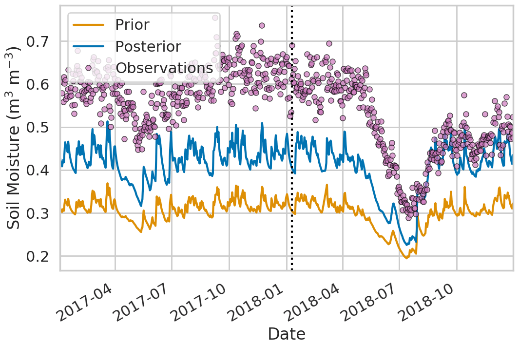
Figure 5Observed and modelled (ensemble mean) soil moisture time series at Gisburn Forest (GISBN). The dotted line separates the period over which observations have been used for assimilation (2017) from the period in which no observations have been assimilated (2018).
Figure 7a shows the KGE values for prior and posterior JULES runs at all 16 sites included in our study. These metrics show how closely the prior and posterior JULES runs match the observations over the period of 2017 and 2018 before and after assimilation of observations from 2017. Figure 7a shows that data assimilation markedly improves the fit to observations at all sites according to the Kling–Gupta metric; all the analysis Kling–Gupta efficiency scores are closer to the ideal value of 1 than the prior values. We note that for all sites, the match between model and measurements is better in 2017 and 2018, even though only observations from 2017 were used in the optimization process. This indicates that the new values for the PTF constants allow JULES to simulate field-scale soil moisture measurements better than the original (prior) PTF constants. Figure 7b shows that the prior and posterior correlation coefficients, r, are very similar at most sites, although there is a slight deterioration of the correlation coefficient at the majority of the sites. Despite this, the reduction in r is very small compared to the overall improvement in the KGE metric at all sites, and the prior and posterior r values are all greater than 0.8 at sites with a typical mineral soil. The r value stays low at Moorhouse (MOORH), perhaps because the soil at this site is too highly organic for the Cosby parameters to really be applicable and for the COSMOS-UK measurements to be reliable. The r value also stays low at Gisburn Forest (GISBN), which is likely due to the fact that there are a large number of trees at this site. The presence of above-ground biomass may make the site-specific calibration less reliable than at other sites (Baatz et al., 2014). The high organic carbon content of the soil at Gisburn Forest likely also contributes to this as our chosen PTF is designed to work best with mineral soils. Interception is another process which potentially complicates the calibration at sites with vegetation, although the authors of Bogena et al. (2013) report that water intercepted by the canopy constitutes a negligible amount of the water detected in the CRNS footprint, even in coniferous forests.
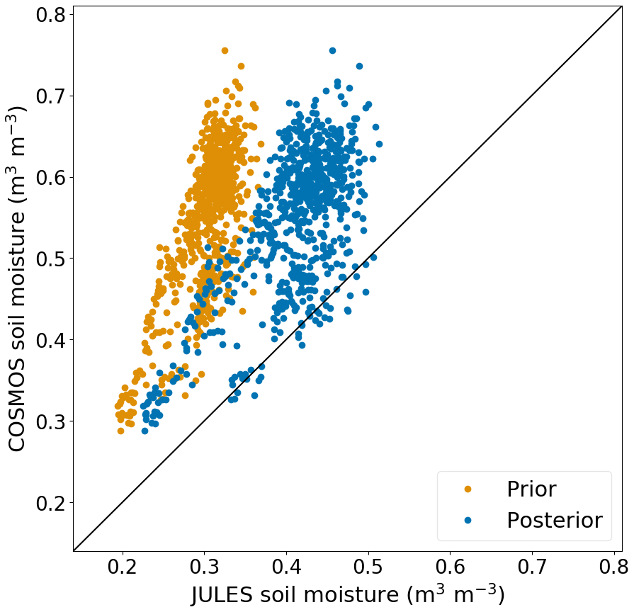
Figure 6Observed vs. modelled (ensemble mean) soil moisture at Gisburn Forest (GISBN) for prior and posterior JULES runs. The diagonal line shows the 1:1 perfect correspondence line. The correlation coefficient at this site changed from 0.73 (prior) to 0.69 (posterior), and the RMSE reduced from 0.25 (prior) to 0.15 (posterior).
Figure 7c shows that a significant contribution to improved KGE at all sites comes from improvement in the alpha component, which is much closer to the ideal value of 1 for all of the posterior JULES runs than the prior JULES runs. The alpha component represents how well the spread in the model matches the spread in the observations. We saw in time series plots such as Figs. 3 and 5 that the spread in JULES soil moisture was too small at all sites; our results show that the data assimilation has acted to correct this by updating the value of the PTF constants. Figure 7d shows that the beta parameter is closer to the ideal value of 1 after data assimilation than before at all sites except for Cardington; i.e. data assimilation is correcting a bias in the JULES outputs at all but one site. The prior bias at Cardington is in the opposite direction to bias at all of the other sites.
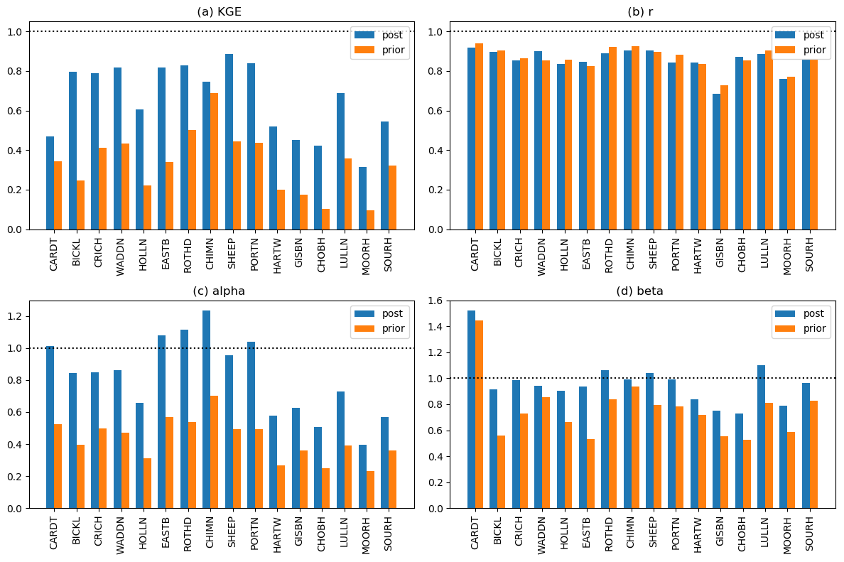
Figure 7Kling–Gupta efficiency scores for JULES runs using prior and posterior PTF variable values. Horizontal dotted lines show the value of the metric for a perfect match between the model and observations.
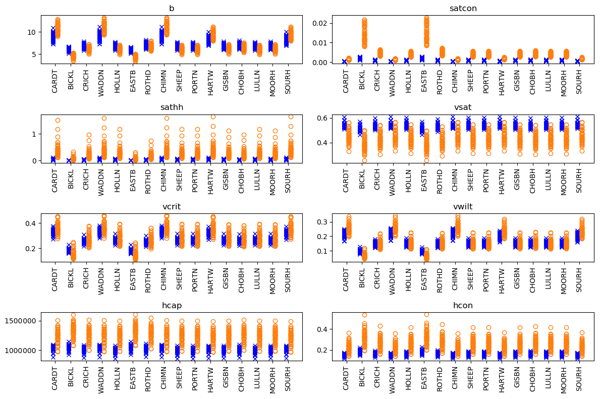
Figure 8Ensemble prior (orange) and posterior (blue) parameter values at each site. These are topsoil results, which we have assumed to correspond to the top two soil layers in JULES (0–35 cm depth from the surface).
3.2 Effect of data assimilation on JULES soil physics parameters
The data assimilation algorithm in this study acts directly on the PTF constants κ1–κ12 which make up the state vector. The resulting changes to the JULES soil physics parameters through Eqs. (4)–(11) are presented here in Sect. 3.2. Figures 8 and 9 show changes to the eight JULES soil physics parameters used for the topsoil and subsoil layers respectively (Sect. 3.3 shows how the underlying PTF constants are updated).
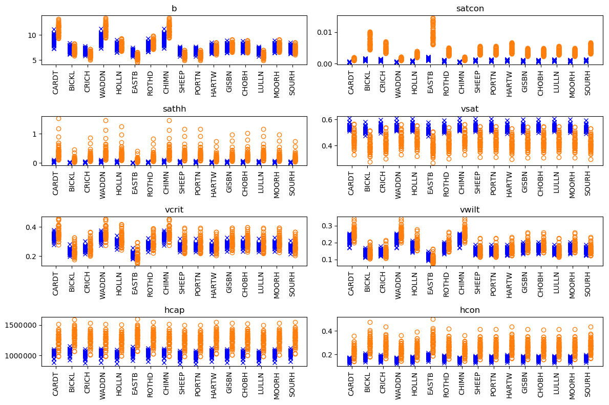
Figure 9Ensemble prior (orange) and posterior (blue) parameter values at each site. These are “subsoil” results, which we have assumed to correspond to the deeper two soil layers in JULES (35–300 cm depth from the surface).
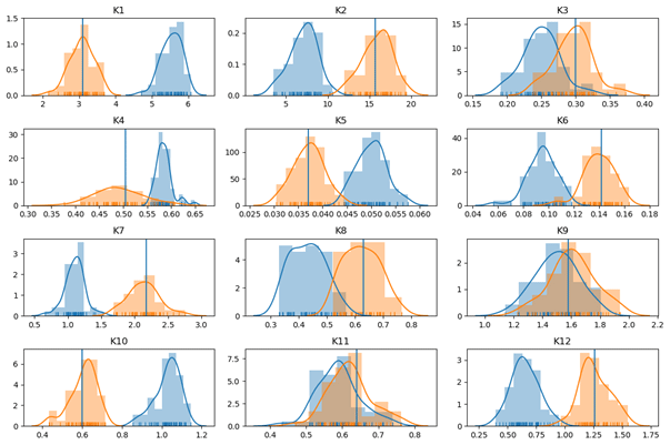
Figure 10Prior and posterior PTF constant value distributions. Orange shows prior and blue posterior. The blue line shows the original value of the constant as in Table 2.
Figures 8 and 9 show that the mean value of Ks (satcon) gets smaller (4 to 5 times smaller) at each site after data assimilation and that the posterior distribution of the Ks (satcon) parameter is narrower than the prior distribution. The results in Figs. 8 and 9 also show that the site-to-site variability of the b parameter reduces following data assimilation; the largest mean prior values of b are reduced, and the distributions with the smallest mean values are shifted to slightly larger values. Figures 8 and 9 show that the mean value θs (vsat) has increased at all the sites following data assimilation, and the distribution of θs (vsat) at each site has become much narrower. The mean values of the θcrit (vcrit) and θwilt (vwilt) distributions have stayed broadly similar or increased slightly after data assimilation. We also see that at all sites Ψs (sathh) becomes very small (∼ 30 times smaller) after data assimilation.
Figures 8 and 9 show that hcap and hcon change through data assimilation. However, this translates into minimal differences between the prior and post soil temperatures; both prior and post data assimilation temperature estimates are close to the in situ COSMOS-UK measurements (not shown).
3.3 Effect of data assimilation on pedotransfer function constants
In this section we present the changes to the 12 PTF constants κ1–κ12. These updates are the direct result of applying the data assimilation algorithm.
Figure 10 shows prior (orange) and posterior (blue) distributions of the 12 PTF constants, κ1 to κ12. These plots demonstrate how the dependence of the soil physics parameters on texture is changed in Eqs. (4) to (11) via data assimilation. The values of κ1, κ2, and κ3 control the magnitude of the soil physics parameter b through Eq. (4). The decreases of κ2 and κ3 after data assimilation translate to a decreased dependence of b on clay and sand fractions through Eq. (4). Changes to κ4, κ5, and κ6 contribute to changes to θs through Eq. (5). The large increase in κ4 values allows larger values of θs to be realized after data assimilation. The parameter Ψs is controlled by κ7, κ8, and κ9. The mean value of κ7 is greatly reduced following data assimilation, and this leads to the much smaller posterior values of Ψs seen in Figs. 8 and 9. The constants κ10, κ11, and κ12 determine the values of Ks through Eq. (7). The shift in the κ10 distribution to larger values leads to the reduction in values of Ks seen in Figs. 8 and 9.
The results in Sect. 3.1 show that we have been able to successfully update the constants in a Cosby-like pedotransfer function based on field-scale in situ soil moisture measurements. The new set of constants obtained in this way generate soil physics parameters at each studied COSMOS-UK site such that there is a large improvement in the match between modelled and observed field-scale soil moisture at all sites.
Our results suggest that it is primarily a combination of the changes to θs, Ψs, and Ks distributions which results in a better match to the observations after data assimilation. Calibrating the PTF using field-scale soil moisture observations allows the model to access higher soil moisture values. We suggest that the data assimilation is effectively acting to slow the drainage of water in JULES, especially close to saturation, by increasing θs and decreasing Ks.
Representation of soil physics processes in land surface models is fundamentally important in modelling soil moisture, and it is important to note that though the soil physics parameter values calculated here fall within a physically reasonable range, they may not exactly match physically expected values for a number of reasons. Firstly, we have generated new soil physics parameters based on field-scale COSMOS-UK measurements; differences in parameter values from the prior values may therefore reflect the different spatial scales over which they were calculated. Additionally, the COSMOS-UK soil moisture observations likely include contributions from processes which are important to soil moisture but we have not taken account of here with JULES, such as ponding of water on the soil surface, interception of water on vegetation, groundwater processes, and local soil compaction. Therefore, we may be effectively correcting for these processes (and others not included in JULES) through our new soil physics parameters. In this experiment we have mainly used grass sites to minimize the impact of vegetation in the daily averaged moisture measurements (JULES outputs show the amount of water intercepted to be, at most, of the order 100 times smaller than the amount of water in the topsoil layer).
The data assimilation is potentially correcting for deficiencies in supporting datasets (such as soil texture information or driving meteorological data) as well as parameter values or process representation in JULES, and we acknowledge that our optimization of the Cosby PTF here relies on consistent soil texture data from the HWSD. When using a land surface model, there is inevitable uncertainty in the soil texture used to generate soil physics parameters. Textures taken from any global dataset, as in this study, are likely inappropriately coarse. On the other hand, soil texture measurements taken at a point will also be unrepresentative of the scales on which land surface models are run. In order to strengthen our conclusions, we repeated our experiment using the SoilGrids soil texture database (Hengl et al., 2017). This gave similar results to the ones shown; optimizing the Cosby PTF produced a better match to the observations at all sites, and we saw a resultant increase in θs (vsat) and reduction in both Ks (satcon) and Ψs (sathh).
Despite these potential limitations, the improvements in soil moisture seen here were obtained by assimilating all the soil moisture values across 16 sites simultaneously rather than on a per-site basis. This strengthens our implicit assumption that the same physical processes can be modelled (through JULES and the Cosby pedotransfer function) for a range of different UK sites and soil types. The fact that one newly optimized PTF improves the fit to data across all 16 sites suggests that this is a systematic improvement to the PTF; i.e. we are improving the mapping between soil texture as reported in the HWSD and soil physics parameters relevant to field-scale application of JULES.
We have shown that it is possible to use the LaVEnDAR data assimilation framework to improve JULES estimates of soil moisture based on 1 year’s worth of field-scale COSMOS-UK soil moisture measurements across 16 sites. We have demonstrated improved fit to observations over a 2-year period at all 16 sites by adjusting the values of constants in the underlying pedotransfer function. Averaging across all the sites, we see an improvement in the average KGE metric from 0.33 (range 0.10 to 0.69) before data assimilation to an average of 0.66 after data assimilation (range 0.31 to 0.89).
The method we propose here for calibrating a PTF using a data assimilation approach could be used for any different choice of land surface model, soil texture data, and/or PTF; our choice of PTF here was motivated by the fact that it is widely used and has a relatively simple mathematical formulation. Calibrating PTFs for the soils on which they are to be used and at the scales at which they are applied, rather than on small-scale field or lab soil samples, will ultimately improve the performance of land surface models. This will allow for better estimates from flood forecasting models, earth system models, and numerical weather prediction.
The code used in these experiments is available from the MetOffice JULES repository (https://code.metoffice.gov.uk/trac/jules, last access: 23 April 2021, Cooper and Pinnington, 2020) under Rose suite number u-bq016. Registration is required. The LaVEnDAR data assimilation first release is available at https://github.com/pyearthsci/lavendar (last access: 23 April 2021, Pinnington, 2019). COSMOS-UK data are deposited annually in the NERC Environmental Information Data Centre (EIDC) (https://doi.org/10.5285/b5c190e4-e35d-40ea-8fbe-598da03a1185, last access: 4 May 2021, Stanley et al., 2021).
EC, EP, and RE devised the experiments, with input from EB and SD. EP created the LaVEnDAR data assimilation framework. EC and EP designed the Rose suite used here and ran the experiments. EC, RE, EP, EB, and SD all contributed to analysis of results. HC provided access to COSMOS-UK data and site-specific information for model setup. EC prepared the manuscript with inputs from all the co-authors.
The authors declare that they have no conflict of interest.
This work was supported by the Natural Environment Research Council (grant no. NE/S017380/1) as part of the Hydro-JULES programme. The authors gratefully acknowledge the provision by UKCEH of hydrometeorological and soil data collected by the COSMOS-UK project. COSMOS-UK is funded by the Natural Environment Research Council (award no. NE/R016429/1) as part of the UK-SCAPE programme.
This research has been supported by the Natural Environment Research Council (grant no. NE/S017380/1).
This paper was edited by Bob Su and reviewed by three anonymous referees.
Antoniou, V., Askquith-Ellis, A., Bagnoli, S., Ball, L., Bennett, E., Blake, J., Boorman, D., Brooks, M., Clarke, M., Cooper, H., Cowan, N., Cumming, A., Doughty, L., Evans, J., Farrand, P., Fry, M., Hewitt, N., Hitt, O., Jenkins, A., Kral, F., Libre, J., Lord, W., Roberts, C., Morrison, R., Parkes, M., Nash, G., Newcomb, J., Rylett, D., Scarlett, P., Singer, A., Stanley, S., Swain, O., Thornton, J., Trill, E., Vincent, H., Ward, H., Warwick, A., Winterbourn, B., and Wright, G.: COSMOS-UK user guide: users' guide to sites, instruments and available data (version 2.10), Tech. Rep., Wallingford, http://nora.nerc.ac.uk/id/eprint/524801/ (last access: 5 August 2020), 2019. a, b, c, d
Baatz, R., Bogena, H., Hendricks Franssen, H.-J., Huisman, J., Qu, W., Montzka, C., and Vereecken, H.: Calibration of a catchment scale cosmic-ray probe network: A comparison of three parameterization methods determination of soil moisture: Measurements and theoretical approaches, J. Hydrol., 516, 231–244, https://doi.org/10.1016/j.jhydrol.2014.02.026, 2014. a, b
Berghuijs, W. R., Harrigan, S., Molnar, P., Slater, L. J., and Kirchner, J. W.: The Relative Importance of Different Flood-Generating Mechanisms Across Europe, Water Resour. Res., 55, 4582–4593, https://doi.org/10.1029/2019WR024841, 2019. a
Best, M. J., Pryor, M., Clark, D. B., Rooney, G. G., Essery, R. L. H., Ménard, C. B., Edwards, J. M., Hendry, M. A., Porson, A., Gedney, N., Mercado, L. M., Sitch, S., Blyth, E., Boucher, O., Cox, P. M., Grimmond, C. S. B., and Harding, R. J.: The Joint UK Land Environment Simulator (JULES), model description – Part 1: Energy and water fluxes, Geosci. Model Dev., 4, 677–699, https://doi.org/10.5194/gmd-4-677-2011, 2011. a, b, c
Bogena, H. R., Huisman, J. A., Baatz, R., Hendricks Franssen, H.-J., and Vereecken, H.: Accuracy of the cosmic-ray soil water content probe in humid forest ecosystems: The worst case scenario, Water Resour. Res., 49, 5778–5791, https://doi.org/10.1002/wrcr.20463, 2013. a
Brooks, R. H. and Corey, A. T.: Hydraulic properties of porous media, Hydrological Papers 3, Colorado State Univ., Fort Collins, 1964. a
Brunetti, G., Šimůnek, J., Bogena, H., Baatz, R., Huisman, J. A., Dahlke, H., and Vereecken, H.: On the Information Content of Cosmic‐Ray Neutron Data in the Inverse Estimation of Soil Hydraulic Properties, Vadose Zone Journal, 18, 1–24, https://doi.org/10.2136/vzj2018.06.0123, 2019. a
Cooper, E. and Pinnington, E.: COSMOS-UK LAVENDAR Rose-suite repository, Met-Office trac system, available at: https://code.metoffice.gov.uk/trac/roses-u/browser/b/q/0/1/6/trunk (last access: 23 April 2021), 2020. a
Cosby, B. J., Hornberger, G. M., Clapp, R. B., and Ginn, T. R.: A Statistical Exploration of the Relationships of Soil Moisture Characteristics to the Physical Properties of Soils, Water Resour. Res., 20, 682–690, https://doi.org/10.1029/WR020i006p00682, 1984. a, b, c, d, e
De Lannoy, G. J. M. and Reichle, R. H.: Assimilation of SMOS brightness temperatures or soil moisture retrievals into a land surface model, Hydrol. Earth Syst. Sci., 20, 4895–4911, https://doi.org/10.5194/hess-20-4895-2016, 2016. a
Dharssi, I., Vidale, P.L.and Verhoef, A., Macpherson, B., Jones, C., and Best, M.: New soil physical properties implemented in the Unified Model at PS18, Met Office Technical Report Series, available at: https://library.metoffice.gov.uk/Portal/Default/en-GB/RecordView/Index/251847( last access: 14 October 2020), 2009. a
Ehsan Bhuiyan, M. A., Nikolopoulos, E. I., Anagnostou, E. N., Polcher, J., Albergel, C., Dutra, E., Fink, G., Martínez-de la Torre, A., and Munier, S.: Assessment of precipitation error propagation in multi-model global water resource reanalysis, Hydrol. Earth Syst. Sci., 23, 1973–1994, https://doi.org/10.5194/hess-23-1973-2019, 2019. a
Evans, J. G., Ward, H. C., Blake, J. R., Hewitt, E. J., Morrison, R., Fry, M., Ball, L. A., Doughty, L. C., Libre, J. W., Hitt, O. E., Rylett, D., Ellis, R. J., Warwick, A. C., Brooks, M., Parkes, M. A., Wright, G. M. H., Singer, A. C., Boorman, D. B., and Jenkins, A.: Soil water content in southern England derived from a cosmic-ray soil moisture observing system – COSMOS-UK, Hydrol. Proc., 30, 4987–4999, https://doi.org/10.1002/hyp.10929, 2016. a, b, c
Fischer, G., Nachtergaele, F., Prieler, S., Van Velthuizen, H., Verelst, L., and Wiberg, D.: Global agro-ecological zones assessment for agriculture (GAEZ 2008), IIASA, Laxenburg, Austria and FAO, Rome, Italy, 10, available at: http://www.fao.org/soils-portal/soil-survey/soil-maps-and-databases/harmonized-world-soil-database-v12/en/ (last access: 5 August 2020), 2008. a
Fowler, A. M., Dance, S. L., and Waller, J. A.: On the interaction of observation and prior error correlations in data assimilation, Q. J. Roy. Meteor. Soc., 144, 48–62, https://doi.org/10.1002/qj.3183, 2018. a
Gupta, H. V., Kling, H., Yilmaz, K. K., and Martinez, G. F.: Decomposition of the mean squared error and NSE performance criteria: Implications for improving hydrological modelling, J. Hydrol., 377, 80–91, https://doi.org/10.1016/j.jhydrol.2009.08.003, 2009. a
Han, X., Franssen, H.-J. H., Rosolem, R., Jin, R., Li, X., and Vereecken, H.: Correction of systematic model forcing bias of CLM using assimilation of cosmic-ray Neutrons and land surface temperature: a study in the Heihe Catchment, China, Hydrol. Earth Syst. Sci., 19, 615–629, https://doi.org/10.5194/hess-19-615-2015, 2015. a
Hengl, T., Mendes de Jesus, J., Heuvelink, G. B. M., Ruiperez Gonzalez, M., Kilibarda, M., Blagotić, A., Shangguan, W., Wright, M. N., Geng, X., Bauer-Marschallinger, B., Guevara, M. A., Vargas, R., MacMillan, R. A., Batjes, N. H., Leenaars, J. G. B., Ribeiro, E., Wheeler, I., Mantel, S., and Kempen, B.: SoilGrids250m: Global gridded soil information based on machine learning, PLOS ONE, 12, 1–40, 2017. a, b
Hilton, F., Collard, A., Guidard, V., Randriamampianina, R., and Schwaerz, M.: ECMWF/EUMETSAT NWP-SAF Workshop on the assimilation of IASI in NWP, Assimilation of IASI Radiances at European NWP Centres, Tech. Rep., available at: https://www.ecmwf.int/sites/default/files/elibrary/2009/9896-assimilation-iasi-radiances-european-nwp-centres.pdf (last access: 5 August 2020), 2009. a
Hodnett, M. G. and Tomasella, J.: Marked differences between van Genuchten soil water-retention parameters for temperate and tropical soils: a new water-retention pedo-transfer functions developed for tropical soils, Geoderma, 108, 155–180, https://doi.org/10.1016/S0016-7061(02)00105-2, 2002. a, b
Holtan, H.: Moisture-tension data for selected soils on experimental watersheds, Agricultural Research Service, U.S. Dept. of Agriculture, 1–11, 1968. a
JULES user guide, A.: JULES documentation, available at: http://jules-lsm.github.io/latest/index.html, last access: 5 August 2020. a
Knoben, W. J. M., Freer, J. E., and Woods, R. A.: Technical note: Inherent benchmark or not? Comparing Nash-Sutcliffe and Kling-Gupta efficiency scores, Hydrol. Earth Syst. Sci., 23, 4323–4331, https://doi.org/10.5194/hess-23-4323-2019, 2019. a, b
Köhli, M., Schrön, M., Zreda, M., Schmidt, U., Dietrich, P., and Zacharias, S.: Footprint characteristics revised for field-scale soil moisture monitoring with cosmic-ray neutrons, Water Resour. Res., 51, 5772–5790, https://doi.org/10.1002/2015WR017169, 2015. a, b
Koster, R., Mahanama, S., Livneh, B., Lettenmaier, D., and Reichle, R.: Skill in streamflow forecasts derived from large-scale estimates of soil moisture and snow, Nat. Geosci., 3, 613–616, https://doi.org/10.1038/ngeo944, 2010. a
Liu, C., Xiao, Q., and Wang, B.: An Ensemble-Based Four-Dimensional Variational Data Assimilation Scheme, Part I: Technical Formulation and Preliminary Test, Monthly Weather Rev., 136, 3363–3373, https://doi.org/10.1175/2008MWR2312.1, 2008. a, b
Liu, Q., Reichle, R. H., Bindlish, R., Cosh, M. H., Crow, W. T., De Jeu, R., De Lannoy, G. J., Huffman, G. J., and Jackson, T. J.: The contributions of precipitation and soil moisture observations to the skill of soil moisture estimates in a land data assimilation system, J. Hydrometeorol., 12, 750–765, https://doi.org/10.1175/JHM-D-10-05000.1, 2011. a
Marthews, T. R., Quesada, C. A., Galbraith, D. R., Malhi, Y., Mullins, C. E., Hodnett, M. G., and Dharssi, I.: High-resolution hydraulic parameter maps for surface soils in tropical South America, Geosci. Model Dev., 7, 711–723, https://doi.org/10.5194/gmd-7-711-2014, 2014. a, b
Martínez-de la Torre, A., Blyth, E. M., and Weedon, G. P.: Using observed river flow data to improve the hydrological functioning of the JULES land surface model (vn4.3) used for regional coupled modelling in Great Britain (UKC2), Geosci. Model Dev., 12, 765–784, https://doi.org/10.5194/gmd-12-765-2019, 2019. a
Mwangi, S., Zeng, Y., Montzka, C., Yu, L., and Su, Z.: Assimilation of Cosmic-Ray Neutron Counts for the Estimation of Soil Ice Content on the Eastern Tibetan Plateau, J. Geophys. Res.-Atmos., 125, e2019JD031529 https://doi.org/10.1029/2019JD031529, 2020. a
Pinnington, E.: pyearthsci/lavendar: First release of LaVEnDAR software (Version v1.0.0), Zenodo, https://doi.org/10.5281/zenodo.2654853 (last access: 23 April 2021), 2019. a
Pinnington, E., Quaife, T., and Black, E.: Impact of remotely sensed soil moisture and precipitation on soil moisture prediction in a data assimilation system with the JULES land surface model, Hydrol. Earth Syst. Sci., 22, 2575–2588, https://doi.org/10.5194/hess-22-2575-2018, 2018. a, b
Pinnington, E., Quaife, T., Lawless, A., Williams, K., Arkebauer, T., and Scoby, D.: The Land Variational Ensemble Data Assimilation Framework: LAVENDAR v1.0.0, Geosci. Model Dev., 13, 55–69, https://doi.org/10.5194/gmd-13-55-2020, 2020. a, b, c
Rawls, W.: Calibration of selected infiltration equations for the Georgia Coastal Plain, 1–15, 1976. a
Ritchie, P. D. L., Harper, A. B., Smith, G. S., Kahana, R., Kendon, E. J., Lewis, H., Fezzi, C., Halleck-Vega, S., Boulton, C. A., Bateman, I. J., and Lenton, T. M.: Large changes in Great Britain's vegetation and agricultural land-use predicted under unmitigated climate change, Environ. Res. Lett., 14, 114012, https://doi.org/10.1088/1748-9326/ab492b, 2019. a
Schaap, M. G., Leij, F. J., and van Genuchten, M. T.: ROSETTA: a computer program for estimating soil hydraulic parameters with hierarchical pedotransfer functions, J. Hydrol., 251, 163–176, https://doi.org/10.1016/S0022-1694(01)00466-8, 2001. a
Seneviratne, S. I., Corti, T., Davin, E. L., Hirschi, M., Jaeger, E. B., Lehner, I., Orlowsky, B., and Teuling, A. J.: Investigating soil moisture–climate interactions in a changing climate: A review, Earth-Sci. Rev., 99, 125–161, https://doi.org/10.1016/j.earscirev.2010.02.004, 2010. a
Shuttleworth, J., Rosolem, R., Zreda, M., and Franz, T.: The COsmic-ray Soil Moisture Interaction Code (COSMIC) for use in data assimilation, Hydrol. Earth Syst. Sci., 17, 3205–3217, https://doi.org/10.5194/hess-17-3205-2013, 2013. a
Stanley, S., Antoniou, V., Askquith-Ellis, A., Ball, L. A., Bennett, E. S., Blake, J. R., Boorman, D. B., Brooks, M., Clarke, M., Cooper, H. M., Cowan, N.; Cumming, A., Evans, J. G., Farrand, P., Fry, M., Hitt, O. E., Lord, W. D., Morrison, R., Nash, G. V., Rylett, D., Scarlett, P. M., Swain, O. D., Szczykulska, M., Thornton, J. L., Trill, E. J., Warwick, A. C., and Winterbourn, B.: Daily and sub-daily hydrometeorological and soil data (2013–2019) [COSMOS-UK], NERC Environmental Information Data Centre [data set], available at: https://doi.org/10.5285/b5c190e4-e35d-40ea-8fbe-598da03a1185, last access: 23 April 2021. a, b, c, d
Van Looy, K., Bouma, J., Herbst, M., Koestel, J., Minasny, B., Mishra, U., Montzka, C., Nemes, A., Pachepsky, Y. A., Padarian, J., Schaap, M. G., Tóth, B., Verhoef, A., Vanderborght, J., van der Ploeg, M. J., Weihermüller, L., Zacharias, S., Zhang, Y., and Vereecken, H.: Pedotransfer Functions in Earth System Science: Challenges and Perspectives, Rev. Geophys., 55, 1199–1256, https://doi.org/10.1002/2017RG000581, 2017. a, b
Wösten, J. H. M., Lilly, A., Nemes, A., and Bas, C. L.: Development and use of a database of hydraulic properties of European soils, Geoderma, 90, 169–185, https://doi.org/10.1016/S0016-7061(98)00132-3, 1999. a
Yang, K., Zhu, L., Chen, Y., Zhao, L., Qin, J., Lu, H., Tang, W., Han, M., Ding, B., and Fang, N.: Land surface model calibration through microwave data assimilation for improving soil moisture simulations, J. Hydrol., 533, 266–276, https://doi.org/10.1016/j.jhydrol.2015.12.018, 2016. a
Zhao, H., Zeng, Y., Lv, S., and Su, Z.: Analysis of soil hydraulic and thermal properties for land surface modeling over the Tibetan Plateau, Earth Syst. Sci. Data, 10, 1031–1061, https://doi.org/10.5194/essd-10-1031-2018, 2018. a