the Creative Commons Attribution 4.0 License.
the Creative Commons Attribution 4.0 License.
 | 07 May 2021
Technical note: Discharge response of a confined aquifer with variable thickness to temporal, nonstationary, random recharge processes
Ching-Min Chang
We-Ci Li
Chi-Ping Lin
I-Hsien Lee
This work develops a transfer function to describe the variation in the integrated specific discharge in response to the temporal variation in the rainfall event in the frequency domain. It is assumed that the rainfall–discharge process takes place in a confined aquifer with variable thickness, and it is treated as nonstationary in time to represent the stochastic nature of the hydrological process. The presented transfer function can be used to quantify the variability in the integrated discharge field induced by the variation in rainfall field or to simulate the discharge response of the system to any varying rainfall input at any time resolution using the convolution model. It is shown that, with the Fourier–Stieltjes representation approach, a closed-form expression for the transfer function in the frequency domain can be obtained, which provides a basis for the analysis of the influence of controlling parameters occurring in the rainfall rate and integrated discharge models on the transfer function.
- Article
(254 KB) - Full-text XML
- BibTeX
- EndNote


Quantifying the variability in the specific discharge response of an aquifer system to fluctuations in inflow recharge is essential for efficient groundwater resources management. However, this requires extensive and continuous hydrological time series data, and these data are very often not available in practice. A possible approach (namely convolution or transfer function approach) to this problem is to simulate the discharge response by convoluting the time-varying recharge input with the corresponding impulse response. In convolution models, the aquifer is regarded as a filter that converts recharge signals into fluctuations of the aquifer head or discharge. Lumped conceptual–convolution models have been shown to be an efficient means for the simulation of the time series of groundwater levels (e.g., Gelhar, 1974; Molénat et al., 1999; Olsthoorn, 2007; Long and Mahler, 2013; Pedretti et al., 2016).
Since the impulse response function in the convolution model contains all information of the system necessary to relate its input to its output, it may be determined from the analytical solution of the linear system equation governing the input–output process (e.g., Cooper and Rorabaugh, 1963). Once a suitable impulse response function can be specified, it allows the simulation of the linear system response to any varying input at any time resolution.
In this work, a regional-scale flow in a confined aquifer with variable thickness, which is recharged by rainfall through an outcrop, is analyzed by deriving transfer functions to characterize the rainfall–discharge process in the frequency domain. The stochastic analysis of groundwater flow is traditionally based on the assumption of the stationarity of the recharge and discharge processes. However, the hydrologic process in nature is nonstationary stochastic (e.g., Christensen and Lettenmaier, 2007; Milly et al., 2008; Sang et al., 2018). In order to improve the quantification of the natural recharge–discharge process, the nonstationary rainfall–discharge process is assumed in this study. The Fourier–Stieltjes representation approach is used to achieve the goal of this work. The analysis of the results is focused on the influence of controlling parameters in the rainfall–discharge models on the transfer function.
In certain areas, aquifer recharge can vary greatly over time, so determining the discharge of the aquifer at the outlet for regional groundwater problems, which involves transferring recharge at the aquifer outcrop over a relatively large space scale, can be quite difficult. However, it is very important for the planning and management of regional groundwater resources that require knowledge of discharge at the aquifer outlet over a long period of time. This study is, therefore, devoted to quantifying the discharge response of the confined aquifer at the outlet to the temporal variation in aquifer recharge.
In this study, a confined aquifer with variable thickness is considered as a linear block box system, with a stochastic rainfall recharge input and, therefore, a stochastic runoff output. Both inputs and outputs are variable in time. In a linear system, the output of the system can be represented as a linear combination of the responses to each of the basic inputs through the convolution integral on a continuous timescale as (e.g., Rugh, 1981; Rinaldo and Marani, 1987) as follows:
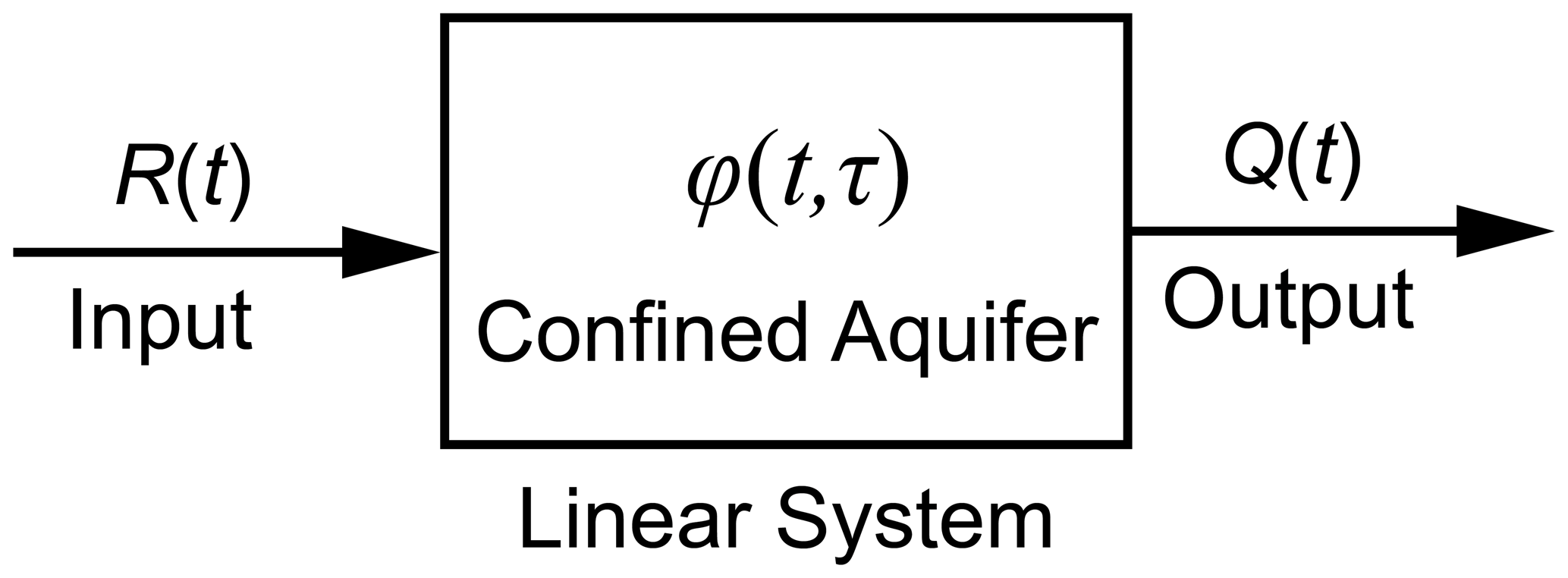
where Q and R denote the output flow (discharge) rate and the input flow (recharge) rate of the system, respectively, and φ is the impulse response function of the system. As shown in Fig. 1, once an appropriate impulse response function can be specified at the scale of the aquifer, it is possible to evaluate the system response from records of the input without the need to specify smaller-scale heterogeneity. As will be shown below, the transfer function of the system can be used to characterize the uncertainty (variability) expected in applying the convolution integral Eq. (1) to the regional groundwater flow problems.
When using the nonstationary Fourier–Stieltjes representations for the perturbed quantities of random recharge and outflow discharge processes, namely (e.g., Priestley, 1965) in the following:
the power spectrum of the mean removed convolution (1) can be written in the following form:
where, in the following:
In Eqs. (2) and (3), Λr and Λq are the oscillatory functions (Priestley, 1965) of the recharge and outflow processes, respectively, ω is the frequency, ξ is a zero-mean random stationary forcing process, which generates the variations in the recharge and, thus, the output flow processes, with an orthogonal increment dZξ. In Eq. (4), Sqq and Sξξ represent the power spectra of the processes q and ξ, respectively, and is termed the transfer function.
In practice, the interest in many cases resides in evaluating the influence of the variation in the recharge on the variation in the outflow discharge. Equation (4) provides an efficient way of quantifying the variability in the outflow induced by the fluctuations in the inflow process in the frequency domain, since it relates the fluctuations in an output time series to those of an input series.
It is worthwhile mentioning that, for the case of second-order stationary rainfall processes, the representations of the forms (2) and (3) are reduced, respectively, to the following:
and, correspondingly, to the following:
where, in the following:
Equations (1) and (4) reveal that, once the transfer function for the linear lumped system is identified, the first two moments of the temporal random discharge fields can be determined. That is, the transfer function approach provides a basic framework for the characterization of large-scale flow processes, which may serve as a basis for an efficient management of groundwater resources. Furthermore, Eq. (4) provides another possible way to identify the aquifer parameters, as it relates the observed fluctuations of an output discharge process to those of a recharge process in the frequency domain.
In the following, the focus is on the development of a closed-form expression for the transfer function for a linear lumped confined flow model in which the regional confined aquifer is directly recharged by rainfall in the area corresponding to the high-elevation outcrop.
The differential equation describing the transient flow of groundwater in inhomogeneous isotropic confined aquifers is of the following form (e.g., Bear, 1979; de Marsily, 1986):
in which Ss represents the specific storage coefficient of the aquifer, ) is the hydraulic head, K(x) is the hydraulic conductivity, and x (= (x1, x2, x3)) is the spatial coordinate vector. Many problems in groundwater flow are regional in nature, with the horizontal extent of the formation being much larger than the vertical extent. It is more practical to regard the flow as essentially horizontal. The regional-scale flow equations can be derived by integrating Eq. (10) along the thickness of the confined aquifer using the assumption of vertical equipotential surfaces (e.g., Bear, 1979; Bear and Cheng, 2010).
Integrating Eq. (10) along the x3 axis perpendicular to the confining beds and using Leibniz's rule results in the following:
where S(x1, x2) is the storage coefficient (or storativity) of the aquifer (=SsB(x1, x2)), B(x1, x2)= b2(x1, x2)−b1(x1, x2) (an aquifer's thickness), b1(x1, x2) and b2(x1, x2) are the elevations of the fixed bottom and ceiling of the confined aquifer, respectively, T(x1, x2) is the transmissivity of the aquifer (=K(x1, x2)B(x1, x2)) interpreted as the depth-integrated hydraulic conductivity, and ) is the depth-averaged hydraulic head defined as follows:
Equation (11) is derived under the following assumptions: (1) there is no exchange of leakage fluxes between the confined aquifer and its confining beds in the direction of x3 axis, (2) h(x1, x2, b2, t) , x2, b1, t) (vertical equipotentials; Bear, 1979; Bear and Cheng, 2010), and (3) all terms involved in the fluxes in the directions of x1 and x2 at the boundaries are removed due to the no-slip condition at the boundaries.
The use of the depth-averaged hydraulic head operator for modeling regional groundwater flow is valid when the variation in aquifer thickness is much smaller than the average thickness (Bear, 1979; Bear and Cheng, 2010). The error introduced by the use of this operator is very small in most cases of practical interest, greatly simplifying the analysis of flow in confined aquifers.
Similarly, when applying Leibniz's rule to the Darcy equation, the vertically integrated specific discharge in the xi direction is given by the following:
In this study, the regional confined aquifer is considered with a nonuniform, unidirectional mean flow in the x1-axis direction but with small flow variations in the x1-axis and x2-axis directions and time-varying recharge at the aquifer outcrop (x1=0). Since the regional flow domain considered in the x1 direction is much larger than that in the x2 direction, Eqs. (11) and (13) can be approximated as one-dimensional by the following:
where , represents the spatial average of the hydraulic conductivity, and R is the recharge rate. It is worth noting that a one-dimensional flow equation with the transmissivity parameter has been widely used to predict the regional groundwater flow fields in the downstream region of the aquifer in field applications (e.g., Gelhar, 1974; Onder, 1998; Molénat et al., 1999; Russian et al., 2013). Equation (14) can be expressed alternatively as follows:
for the convenient analysis of the effect of the thickness of the aquifer.
In the following analysis, the recharge rate is considered a random function of time. Equation (15) is then regarded as a stochastic differential equation with a stochastic input in time and, therefore, a stochastic output in time. Introduction of the decomposition of the depth-averaged hydraulic head into a mean and zero-mean perturbation into Eq. (16), after subtracting the mean of the resulting equation from Eq. (16), means that the result is the following equation describing the depth-averaged head perturbation:
where is the fluctuations in depth-averaged head.
If it is assumed that the thickness of the confined aquifer increases exponentially in the x direction, in accordance with Hantush (1962) and Marino and Luthin (1982), as follows:
then Eq. (17) becomes the following:
In Eq. (18), β and α are positive geometrical parameters. Furthermore, the outcrop (x=0) and outlet (x=L) of the confined aquifer are considered as constant head boundaries. Since Eq. (19) only quantifies the response of the depth-averaged head to changes in the recharge rate, the initial and boundary conditions for Eq. (19) may be represented as follows:
The following Fourier–Stieltjes integral representation of a depth-averaged head process is used to solve Eqs. (19) and (20) for the fluctuations h′ in terms of r:
where Λh is the oscillatory function of depth-averaged head process. The resulting differential equation for the oscillatory functions is found from using Eqs. (2) and (21) in Eqs. (19) and (20) as follows:
with the following conditions:
By solving the above boundary value problem, the oscillatory function of depth-averaged head process is found to be the following (see Appendix A):
where μ=αL and ). It implies from Eqs. (3), (15) and (24) that, at the arbitrary location x=xε, one finds the following:
where . This means that the impulse response function of the system φ in Eqs. (1) or (5) is taken in the following form:
Equation (25) implies that the transfer function depends on the oscillatory function of the temporal random rainfall process; consequently, to complete the analysis of the transfer function, the oscillatory function of the temporal random rainfall process must be specified. It is assumed that the generated temporal random perturbations of the rainfall field are governed by the noise-forced diffusive rainfall model (North et al., 1993) as follows:
where ρ is a zero-mean rainfall rate perturbation, τ0 and λ0 are the characteristic timescales and length scales, respectively, which are inherent to the rainfall field, and ξ is a zero-mean random stationary forcing process which has a spectral representation of the following form (e.g., Lumley and Panofsky, 1964):
In Eq. (27), the rainfall rate field is represented as a first-order continuous autoregressive process in time and an isotropic second-order autoregressive process in space.
Furthermore, the rest of this study takes into account that rain falls within a defined period of time over a certain area of horizontal extension from to x=ℓ. As such, the initial and boundary conditions for rainfall rate perturbations may be represented by the following:
4.1 Nonstationary random rainfall fields in time
Using the Fourier–Stieltjes integral representation for the perturbation ρ, as follows:
and Eq. (28) in Eq. (27), it follows that:
where Λρ is the oscillatory function of the rainfall rate processes. With the application of the initial and boundary conditions, as follows:
the solution of Eqs. (31) and (32) is given by the following (see Appendix B):
where , , Ωt=ωt, and Γ=ωτ0.
In the case where the regional confined aquifer is directly recharged by rainfall at the aquifer outcrop (x=0), the oscillatory function is reduced to the following:
Correspondingly, the power spectrum of the rainfall rate, Srr(t, ω), can be expressed by the following:
where T1= exp[], T2= exp(), and T3 = exp().
The transfer function of the rainfall processes in Eq. (35) behaves like a filter, attenuating the high-frequency part of the rainfall spectrum. The graph of the transfer function, which is characterized by the characteristic timescale τ0 for different characteristic length scales, is shown in Fig. 2. It clearly shows a reduction in the transfer function with increasing τ0, implying a reduction in the variability in the rainfall field with the characteristic timescale of the rainfall field. A larger τ0 decreases the temporal persistence of the rainfall fluctuations, resulting in a smaller transfer function. It is also seen that, for a fixed value of the timescale, the transfer function of the rainfall processes tends to decrease as the length scale of the rainfall field increases. The influence of the length scale plays a similar role to the influence of the timescale in reducing the temporal persistence of the rainfall fluctuations and, thus, the variability in the rainfall field.
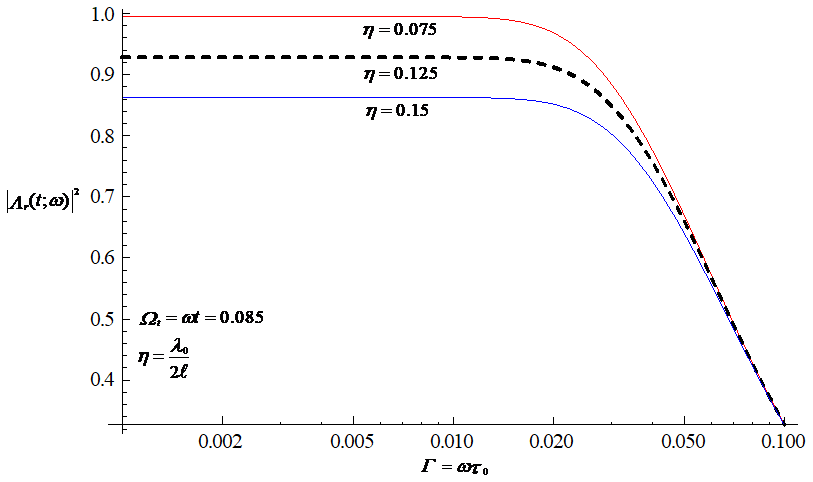
Figure 2Graphical representation of the transfer function of the rainfall processes in Eq. (35) characterized by the timescale for different length scales, where the series calculation is truncated up to 100.
Through the use of Eqs. (25) and (34), the oscillatory function of the integrated discharge process could be represented as follows:
Thus, the transfer function of the integrated discharge flux takes the following form:
where , and in the following:
Note that the linearity in modeling the recharge–discharge response of a catchment in Eq. (1), which was originally developed for large catchments, increases with catchment area (e.g., Chow et al., 1988). This implies that the impulse responses and transfer functions derived here are valid in large, confined aquifers.
An essential feature of the transfer function of the integrated discharge flux in Eq. (37) is the resulting filtering associated with the flow process, as shown in Fig. 3. The attenuation of the high-frequency part of the flow discharge spectrum means that the flow process smooths out much of the small-scale variations caused by the rainfall field. Physically, this feature implies that the flow field is much smoother than the rainfall field. The figure also shows that the transfer function at fixed values for frequency and time increases with the increasing thickness of the confined aquifer. An increase in the thickness of the aquifer leads to an increased temporal persistence of the flow discharge fluctuations caused by the variation in the rainfall field and, thus, to an increase in the variability in integrated discharge field. As shown in Fig. 4, the ratio of the mean hydraulic conductivity to the storage coefficient (often referred to as the aquifer diffusivity) plays a similar role in influencing the variation in the transfer function to the thickness of the confined aquifer. The introduction of a larger aquifer diffusivity leads to a larger transfer function of integrated discharge and, thus, to a larger variability in the discharge field. Since the variability in the discharge field is positively correlated with that of rainfall field, the variability in the integrated discharge field will decrease with the increasing characteristic timescale or length scale of the rainfall field (see Fig. 2).
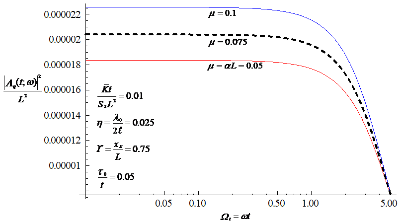
Figure 3Influence of the thickness of the confined aquifer on the transfer function of the discharge flux, where the series calculation is truncated up to 100.

Figure 4Influence of the aquifer diffusivity on the transfer function of the discharge flux, where the series calculation is truncated up to 100.
From Eqs. (4) or (8), the transfer function can be defined as the ratio of the fluctuations of an observation of output time series to those of input time series in a frequency domain. Equations (35) and (37) indicate that the transfer functions are related to the properties of the rainfall field and the aquifer, such as the characteristic scales of the time and length of the rainfall field and the diffusivity and thickness parameters of the aquifer. Therefore, the transfer function derived here has the potential to perform a parameter estimation based on the observations of input and output time series using the inverse modeling approach.
The traditional approach to regional groundwater flow problems introduces the transmissivity term, namely the depth-integrated hydraulic conductivity operator, as follows:
into to the groundwater flow equation (diffusion equation) to reduce the three-dimensional equation to a two-dimensional one as follows:
This means that the effects of both the variation in K in x3 direction and the aquifer thickness are implicitly reflected in the term T(x1, x2). This leads to great difficulties in assessing the influence of aquifer thickness on the flow field with Eq. (40).
The proposed diffusion equation of this work is the following:
which, when derived by the hydraulic approach (Bear, 1979; Bear and Cheng, 2010), provides an efficient way of analyzing flow fields in confined aquifers of nonuniform thickness. Note that Eq. (41) is the reformulation of Eq. (11). In addition, the usual observations of flow in porous media are measurements of hydraulic head from wells screened over extended sections of the medium. The measurement at a given location approximately represents a depth-averaged actual hydraulic head resulting from flow through a three-dimensional hydraulic conductivity field across the thickness of the medium. This means that the depth-averaged head representation used in Eq. (41) is consistent with what is observed in the fields.
Climate changes have a direct influence on the rainfall event (e.g., Trenberth, 2011; Pendergrass et al., 2014; Eekhout et al., 2018). The nonstationarity in the statistical properties of a rainfall field is a representation of climate change (e.g., Razavi et al., 2015; López and Francés, 2013; Benoit et al., 2020). The nonstationary effect of climatic change over time on variability in groundwater-specific discharge has not yet been well characterized. The transfer function in Eq. (37), which relates the nonstationary spectra of the rainfall fluctuations to those of integrated discharge variation, generalizes existing studies that considered stationary recharge and discharge fields. To our knowledge, it has not been previously presented in the literature and has the potential for analyzing the effects of climate change on temporal groundwater-specific discharge variability.
4.2 Application in the prediction of outflow discharge
The usefulness of the stochastic theory presented here lies in its essentially predictive nature. The variance can be used as a quantification of the uncertainty associated with the prediction in field situations using the linear system model. In this sense, the solution of Eq. (1) ±, i.e., two times the square root of the variance, provides a rational framework for predicting discharge over a relatively large spatial scale where direct observations of such a dependent variable are not possible.
For large times, the first term in Eq. (37) dominates the sum of the other terms, and therefore, the transfer function can be approximated by the following:
where Θ1= 1+π2η2, ), Ξ= (), ), and TA= exp(). If the variation in the rainfall event is generated by a random white noise forcing, the variance in the outflow discharge at large timescales can then be calculated using Eq. (42) as follows:
where G0 represents a constant spectral density of a white noise process. Note that white noise is a signal that contains all frequencies in equal proportions; that is, a signal for which the spectrum is flat.
After observing the recharge rate R(t) over time at the outcrop of the aquifer and identifying input parameters, such as the specific storage coefficient, mean hydraulic conductivity and geometrical parameters of the aquifer and the characteristic timescales and length scales of the rainfall event for a given area or region, the discharge can be determined under uncertainty in the far downstream aquifer area, i.e., Eq. (1) together with Eq. (26) ± being two times the square root of Eq. (43). It provides an important basis for the rational management of regional groundwater resources in complex geologic settings under uncertainty.
4.3 A note on stationary random rainfall fields in time
If the temporal random rainfall fields are stationary, there exists a representation of the rainfall perturbation process in terms of a Fourier–Stieltjes integral in the form of Eq. (6). Substituting Eqs. (6) and (21) into Eq. (19) gives the following:
The solution of Eq. (44) with conditions Eq. (23) is as follows:
so that, in the following:
and, thus, in the following:
where, in the following:
Δ1= exp[-(θm+θn)t], Δ2= exp(−θmt) + exp(−θnt), and Δ3= exp(−θmt)-exp(−θnt).
At large timescales, Eq. (35) approaches a finite value as follows:
and the corresponding rainfall process is stationary. Combining Eqs. (47) with (49) gives the following:
Note that the nonstationarity in the hydraulic head or integrated discharge is introduced by a nonuniform thickness of the confined aquifer, even if the recharge field is stationary. Nonuniformity in the mean flow, for example, can also cause the nonstationarity in the statistics of random flow fields in heterogeneous aquifers (e.g., Rubin and Bellin, 1994; Ni and Li, 2006; Ni et al., 2010).
An analytical transfer function is developed to describe the spectral response characteristics of confined aquifers with variable thickness to the variation in the rainfall field, where the aquifer is directly recharged by rainfall at the outcrop of the aquifer. The rainfall–discharge process is treated as nonstationary in time, as it reflects the stochastic nature of the hydrological process. Any varying rainfall input at any time resolution can be convolved with the transfer function (or impulse response function) to simulate any discharge output of a linear model. The transfer function derived here, which relates the nonstationary spectra of the rainfall fluctuations to those of integrated discharge variation, has the potential to analyze the influence of climate change on groundwater recharge variability.
The closed-form results of this work are developed on the basis of the Fourier–Stieltjes representation approach, which allows us to analyze the effects of the controlling parameters in the models on the transfer function of the integrated discharge. It is found that the persistence in rainfall fluctuations is greater for a smaller value of the characteristic timescale or length scale of the rainfall field, which, in turn, leads to greater variability in the integrated discharge field. The attenuating characteristic of the confined aquifer flow system is observed in the spectral domain. The variability in the integrated discharge in a confined aquifer with variable thickness is increased with the thickness parameter α. The larger the aquifer diffusivity, the greater the spectrum (variability) of the integrated discharge.
The boundary value problem describing the depth-averaged head fluctuations induced by the variation in recharge rate in frequency domain is given by Eqs. (22) and (23). Using the transformation, as follows:
Equation (22) in Λh(x, t; ω), together with Eq. (23), can be converted into a new (easier) one with a new variable U(x, t; ω) as follows:
with the following:
The solution of Eqs. (A2) and (A3) can be found through the technique of the separation of variables (e.g., Farlow, 1993) as follows:
where ). With reference to Eq. (A1), the solution to Eqs. (22) and (23) is then given by Eq. (24).
Making use of the following transformation:
leads Eqs. (31) and (32) to the following:
with the following:
In a similar way, based on the technique of the separation of variables, Eqs. (B2) and (B3) arrive at the solution in the following form:
where ςm=m2π2η2, η= ), , and Γ=ωτ0. The use of Eqs. (B1) and (B4) results in Eq. (33).
No data sets were used in this article.
CMC, CFN, WCL, CPL and IHL conceptualized the paper, developed the methodology, conducted the formal analysis, prepared the original draft and reviewed and edited the paper. CFN also supervised the project and acquired the funding.
The authors declare that they have no conflict of interest.
Research leading to this paper has been partially supported by the Taiwan Ministry of Science and Technology (grant nos. MOST 108-2638-E-008-001-MY2, MOST 108-2625-M-008-007, and MOST 107-2116-M-008-003-MY2. We are grateful to the editor, Nadia Ursino, and the anonymous referees for the constructive comments that improved the quality of this work.
This research has been supported by the Ministry of Science and Technology, Taiwan (grant nos. MOST 108-2638-E-008-001-MY2, MOST 108-2625-M-008-007, and MOST 107-2116-M-008-003-MY2).
This paper was edited by Nadia Ursino and reviewed by two anonymous referees.
Bear, J.: Hydraulics of groundwater, McGraw-Hill, New York, 1979.
Bear, J. and Cheng, A. H.-D.: Modeling groundwater flow and contaminant transport, Springer, Dordrecht, 2010.
Benoit, L., Vrac, M., and Mariethoz, G.: Nonstationary stochastic rain type generation: accounting for climate drivers, Hydrol. Earth Syst. Sci., 24, 2841–2854, https://doi.org/10.5194/hess-24-2841-2020, 2020.
Christensen, N. S. and Lettenmaier, D. P.: A multimodel ensemble approach to assessment of climate change impacts on the hydrology and water resources of the Colorado River Basin, Hydrol. Earth Syst. Sci., 11, 1417–1434, https://doi.org/10.5194/hess-11-1417-2007, 2007.
Chow, V. T., Maidment, D. R., and Mays, L. W.: Applied hydrology, McGraw-Hill, New York, 1988.
Cooper, H. H. and Rorabaugh, M. J.: Ground water movements and bank storage due to flood stages in surface streams, USGS Water Supply Paper 1536-J. Reston, Virginia, USGS, 1963.
de Marsily, G.: Quantitative hydrogeology: Groundwater hydrology for engineers, Academic Press, Orlando, FL, 1986.
Eekhout, J. P. C., Hunink, J. E., Terink, W., and de Vente, J.: Why increased extreme precipitation under climate change negatively affects water security, Hydrol. Earth Syst. Sci., 22, 5935–5946, https://doi.org/10.5194/hess-22-5935-2018, 2018.
Farlow, S. J.: Partial differential equations for scientists and engineers, Dover, New York, N.Y., 1993.
Gelhar, L. W.: Stochastic analysis of phreatic aquifer, Water Resour. Res., 10, 539–545, 1974.
Hantush, M. S.: Flow of ground water in sands of nonuniform thickness: 3. Flow to wells, J. Geophys. Res., 67, 1527–1534, 1962.
Long, A. J. and Mahler, B. J.: Prediction, time variance, and classification of hydraulic response to recharge in two karst aquifers, Hydrol. Earth Syst. Sci., 17, 281–294, https://doi.org/10.5194/hess-17-281-2013, 2013.
López, J. and Francés, F.: Non-stationary flood frequency analysis in continental Spanish rivers, using climate and reservoir indices as external covariates, Hydrol. Earth Syst. Sci., 17, 3189–3203, https://doi.org/10.5194/hess-17-3189-2013, 2013.
Lumley, J. L. and Panofsky, H. A.: The structure of atmospheric turbulence, John Wiley, New York, 1964.
Marino, M. A. and Luthin, J. N.: Seepage and Groundwater, Elsevier, New York, 1982.
Milly, P. C. D., Betancourt, J., Falkenmark, M., Hirsch, R. M., Kundzewicz, Z. W., Lettenmaier, D. P., and Stouffer, R. J.: Stationarity is Dead: Whither water management?, Science, 319, 573–574, 2008.
Molénat, J., Davy, P., Gascuel-Odoux, C., and Durand, P.: Study of three subsurface hydrological systems based on spectral and cross-spectral analysis of time series, J. Hydrol., 222, 152–164, 1999.
Ni, C.-F. and Li, S.-G.: Modeling groundwater velocity uncertainty in nonstationary composite porous media, Adv. Water Resour., 29, 1866–1875, 2006.
Ni, C.-F., Li, S.-G., Liu, C.-J., and Hsu, S. M.: Efficient conceptual framework to quantify flow uncertainty in large-scale, highly nonstationary groundwater systems, J. Hydrol., 381, 297–307, 2010.
North, G. R., Shen, S. S. P., and Upson, R. B.: Sampling errors in rainfall estimates by multiple satellites, J. Appl. Meteorol., 32, 399–410, 1993.
Olsthoorn, T.: Do a bit more with convolution, Groundwater, 46, 13–22, 2007.
Onder, H.: One-dimensional transient flow in a finite fractured aquifer system, Hydrolog. Sci. J., 43, 243–265, 1998.
Pedretti, D., Russian, A., Sanchez-Vila, X., and Dentz, M.: Scale dependence of the hydraulic properties of a fractured aquifer estimated using transfer functions, Water Resour. Res., 52, 5008–5024, 2016.
Pendergrass, A. G. and Hartmann, D. L.: Changes in the distribution of rain frequency and intensity in response to global warming, J. Climate, 27, 8372–8383, 2014.
Priestley, M. B.: Evolutionary spectra and non-stationary processes, J. R. Stat. Soc. B Met., 27, 204–237, 1965.
Razavi, S., Elshorbagy, A., Wheater, H., and Sauchyn, D.: Toward understanding nonstationarity in climate and hydrology through tree ring proxy records, Water Resour. Res., 51, 1813–1830, 2015.
Rinaldo, A. and Marani, A.: Basin scale model of solute transport, Water Resour. Res., 23, 2107–2118, 1987.
Rubin, Y. and Bellin, A.: The effects of recharge on flow nonuniformity and macrodispersion, Water Resour. Res., 30, 939–948, 1994.
Rugh, W. J.: Nonlinear system theory: the Volterra/Wiener approach, Johns Hopkins University Press, Baltimore, 1981.
Russian, A., Dentz, M., Le Borgne, T., Carrera, J., and Jimenez-Martinez, J.: Temporal scaling of groundwater discharge in dual and multicontinuum catchment models, Water Resour. Res., 49, 8552–8564, 2013.
Sang, Y.-F., Sun, F., Singh, V. P., Xie, P., and Sun, J.: A discrete wavelet spectrum approach for identifying non-monotonic trends in hydroclimate data, Hydrol. Earth Syst. Sci., 22, 757–766, https://doi.org/10.5194/hess-22-757-2018, 2018.
Trenberth, K.: Changes in precipitation with climate change, Clim. Res., 47, 123-138, 2011.
- Abstract
- Introduction
- Problem formulation
- Theoretical development
- Results and discussion
- Conclusions
- Appendix A: Evaluation of Λh in Eq. (20)
- Appendix B: Evaluation of Λρ in Eq. (31)
- Data availability
- Author contributions
- Competing interests
- Acknowledgements
- Financial support
- Review statement
- References