the Creative Commons Attribution 4.0 License.
the Creative Commons Attribution 4.0 License.
 | 15 Jan 2021
Hillslope and groundwater contributions to streamflow in a Rocky Mountain watershed underlain by glacial till and fractured sedimentary bedrock
Sheena A. Spencer
Axel E. Anderson
Uldis Silins
Adrian L. Collins
Permeable sedimentary bedrock overlain by glacial till leads to large storage capacities and complex subsurface flow pathways in the Canadian Rocky Mountain region. While some inferences on the storage and release of water can be drawn from conceptualizations of runoff generation (e.g., runoff thresholds and hydrologic connectivity) in physically similar watersheds, relatively little research has been conducted in snow-dominated watersheds with multilayered permeable substrates that are characteristic of the Canadian Rocky Mountains. Stream water and source water (rain, snowmelt, soil water, hillslope groundwater, till groundwater, and bedrock groundwater) were sampled in four sub-watersheds (Star West Lower, Star West Upper, Star East Lower, and Star East Upper) in Star Creek, SW Alberta, to characterize the spatial and temporal variation in source water contributions to streamflow in upper and lower reaches of this watershed. Principal component analysis was used to determine the relative dominance and timing of source water contributions to streamflow over the 2014 and 2015 hydrologic seasons. An initial displacement of water stored in the hillslope over winter (reacted water rather than unreacted snowmelt and rainfall) occurred at the onset of snowmelt before stream discharge responded significantly. This was followed by a dilution effect as snowmelt saturated the landscape, recharged groundwater, and connected the hillslopes to the stream. Fall baseflows were dominated by either riparian water or hillslope groundwater in Star West. Conversely, in Star East, the composition of stream water was similar to hillslope water in August but plotted outside the boundary of the measured sources in September and October. The chemical composition of groundwater seeps followed the same temporal trend as stream water, but the consistently cold temperatures of the seeps suggested deep groundwater was likely the source of this late fall streamflow. Temperature and chemical signatures of groundwater seeps also suggest highly complex subsurface flow pathways. The insights gained from this research help improve our understanding of the processes by which water is stored and released from watersheds with multilayered subsurface structures.
- Article
(4102 KB) - Full-text XML
- BibTeX
- EndNote


Forest disturbance from wildfire, pathogens, or forest harvesting removes the forest canopy, increasing the total precipitation that reaches the forest floor (Williams et al., 2019; Burles and Boon, 2011; Boon, 2012; Pugh and Small, 2012; Varhola et al., 2010), often altering the dominant flow pathways, increasing streamflow quantity, and changing the timing of flows in forested watersheds (Stednick, 1996; Scott, 1993; Bearup et al., 2014; Winkler et al., 2017). However, large variability has been observed in streamflow responses following disturbance due to differences in disturbance type, vegetation type, precipitation regimes, and soil moisture storage (Brown et al., 2005; Stednick, 1996). Some studies in Alberta's Rocky Mountains have reported little, if any, change in streamflow following disturbance (Williams et al., 2015; Harder et al., 2015; Goodbrand and Anderson, 2016; Andres et al., 1987), but the mechanisms and watershed features (e.g., bedrock, surficial geology, and wetlands) potentially responsible for the lack of flow response have received little attention. It has been suggested that watersheds exhibiting a lack of change in streamflow following disturbance might be associated with a large storage capacity and complex subsurface flow pathways (Harder et al., 2015), but the higher-order controls regulating these muted responses remain unclear.
Runoff generation has been extensively studied in regions with relatively impermeable bedrock overlain by shallower soils, which has led to broadly accepted conceptualizations of runoff dynamics (e.g., old water contributions to streamflow, macropore flow, and subsurface streamflow generation – McGlynn et al., 2002; fill and spill hypothesis – Tromp-van Meerveld and McDonnell, 2006; hillslope–stream connectivity – Jencso et al., 2009). However, these conceptualizations may not apply to regions with more complex structural controls on runoff such as permeable bedrock, deeper soils, or where multiple subsurface systems interact. Runoff generation in Alberta's Rocky Mountains has added complexity because of the combination of both permeable sedimentary bedrock (highly fractured and faulted) and an overlying layer of deep, heterogenous glacial till (3 m deep, on average, and up to 10 m deep; AGS, 2004; Waterline Resources Inc., 2013). This is in contrast to regions such as the southern Rocky Mountains in Colorado (Sueker et al., 2000; Cowie et al., 2017) and Montana (Jencso et al., 2009, 2010; Nippgen et al., 2015) that are often dominated by less permeable metamorphic or igneous bedrock and thinner soils. While runoff generation processes may differ from these regions, some inferences can be drawn from studies in regions with either permeable bedrock or deep soils alone. Watersheds with high bedrock permeability have been associated with longer subsurface flow pathways and the slow release of stored water to streams during baseflow (Uchida et al., 2006; Liu et al., 2004; Pfister et al., 2017). Uchida et al. (2006) reported that a watershed with greater bedrock permeability had larger aquifer storage, and the subsequent release of stored water maintained baseflow later in the year. Similarly, Liu et al. (2004) showed that the recession limb of the annual hydrograph in the Colorado front range Rocky Mountains was driven by baseflow released from fractured bedrock, but Cowie et al. (2017) also stressed the importance of talus slopes as a source of streamflow in the same alpine watershed. Deep soils and till deposits with large storage capacities have also been shown to sustain baseflows during drier periods (Floriancic et al., 2018; Shanley et al., 2015). Deep sediment deposits in the Poschiavino watershed, in Switzerland, were associated with greater storage capacity and higher winter baseflows compared to watersheds with shallow sediment deposits (Floriancic et al., 2018). Similarly, deep basal till in the Sleepers River watershed in Vermont was associated with large storage capacity and low permeability that promoted the extended maintenance of baseflow (Shanley et al., 2015).
While these studies illustrate the influence of permeable or fractured bedrock, deep soils, or till on baseflows, few studies have explored the combination of these storage zones on streamflow contributions (Burns et al., 1998; Dalke et al., 2012; Shaman et al., 2004). Burns et al. (1998) characterized the difference in deep (bedrock) and shallow (soils and till) flow systems in the Catskill Mountains in New York, a region with both glacial till and permeable sedimentary bedrock. Baseflow was maintained by discharge from perennial springs which originated from bedrock fractures, rather than contributions from the soil and till flow system (Burns et al., 1998). Conversely, fragipan layers contributed to differing flow systems under dry vs. wet antecedent conditions in central New York (state), USA (Dalke et al., 2012). Storm flow was generated from deep flow pathways below the fragipan during dry conditions and near surface flow pathways during wet conditions. Comparatively little research on runoff generation processes has been conducted in the Canadian Rocky Mountains, in part due to deep snow that is present for much of the year (October–May). While some studies have shown the importance of groundwater contributions to streamflow in alpine watersheds in the Rocky Mountains (Hood and Hayashi, 2015; McClymont et al., 2010), the additional complexity imposed by highly heterogeneous glacial till and permeable bedrock in sub-alpine and upper montane watersheds has limited more extensive research on runoff dynamics of this region. As a first attempt to conceptualize runoff generation in Alberta's Rocky Mountains, Spencer et al. (2019) quantified storage and precipitation–runoff relationships from hydrometric data. Results indicated that runoff generation was strongly governed by the interaction of two zones of storage – soil and till storage and bedrock storage. The alpine region and sub-alpine/upper montane region were also identified as two separate hydrologic response units that differed in timing and flow pathways for runoff response. While Spencer et al. (2019) developed a conceptualization of runoff generation for this region, they concluded that coupled flow and tracer approaches would be needed to reduce uncertainty in estimated flow contributions from each storage zone.
Chemical signatures of source water (rain, snowmelt, soil water, hillslope groundwater, till groundwater, and bedrock groundwater) and stream water can be used to determine which sources are contributing to streamflow during different flow conditions using end-member mixing analysis (EMMA; Christophersen and Hooper, 1992). The key assumptions for EMMA are that (1) the tracers are conservative, (2) the mixing process is linear, (3) source chemistry does not change temporally or spatially over the period or area studied (Inamdar, 2011; Hooper, 2003), and (4) all sources have been identified and have the potential to contribute to streamflow. Many studies have used EMMA to conceptualize when different geologic components are contributing to the stream (e.g., James and Roulet, 2006; Cowie et al., 2017; Ali et al., 2010). However, this approach has been most successful in smaller watersheds (1 km2) because of more constrained variation in source water at smaller spatial scales (Hoeg et al., 2000). Large watersheds could be characterized based on smaller sub-watersheds (James and Roulet, 2006) if the sub-watersheds are homogeneous. Others have concluded that where source water displays large variation or assumptions cannot be met, runoff processes should be described qualitatively (Inamdar et al., 2013; Hoeg et al., 2000; Correa et al., 2019).
To expand on recent work carried out in the same study area by Spencer et al. (2019), this study aims to advance the conceptualization of runoff generation in the Rocky Mountains in Alberta, Canada. The objectives of this study were to (1) characterize how sources of stream water (rain, snowmelt, soil water, hillslope groundwater, till groundwater, and bedrock groundwater) vary spatially, across four sub-watersheds of a Rocky Mountain watershed, and temporally, from spring snowmelt to the start of the next year's snow accumulation period, and (2) determine the relative contributions of source water to the stream from spring to fall for each sub-watershed. This study should help inform the current conceptualization of runoff generation in northern Rocky Mountain watersheds.
Star Creek watershed (10.4 km2; Fig. 1) is located in the eastern slopes of Canada's Rocky Mountains, a region with fractured sedimentary bedrock overlain by glacial till. Average annual precipitation was 720 mm at Star Main (1482 m above sea level – a.s.l.) and 990 mm at Star Alpine (1732 m a.s.l.; Spencer et al., 2019). The area-weighted average annual precipitation (2005–2018) was 950 mm, using the Thiessen polygon method and nine precipitation gauges at a range of elevations in and surrounding Star Creek; 50 %–60 % of the precipitation falls in the form of snow (Spencer et al., 2019). Soils are Eutric Brunisols (Canadian System of Soil Classification; also known as Eutric Cambisols in the Food and Agriculture Organization system) approximately 1 m deep, on average. Star Creek is underlain by unsorted and uncompacted glacial till, which is generally less than 3 m deep with an estimated total area of 2.4 km2 (AGS, 2004; Fig. 1). Some clay-rich till layers, likely from localized glacial ice melt features, occur intermittently throughout the watershed, resulting in heterogeneous and uneven distribution of glacial till throughout the watershed. Sedimentary geologic formations (Upper Paleozoic formation, Belly River–St. Mary Succession, and Alberta Group formation) are primarily composed of shale and sandstone (AGS, 2004) and are highly fractured due to folding and faulting (Waterline Resources Inc., 2013).

Figure 1Star Creek watershed. Suction lysimeter and hillslope groundwater well locations are magnified in green boxes.
Star Creek includes two main sub-watersheds, namely Star East (3.9 km2; 1537–2628 m a.s.l.) and Star West (4.6 km2; 1540–2516 m a.s.l.). Unvegetated talus slopes (0.50 km2 in Star East and 0.53 km2 in Star West, digitized from orthoimages) and exposed bedrock form the upper portion of alpine zones in both sub-watersheds (Figs. 1 and 2). Talus slopes terminate in the alpine and transitional forested regions of the watershed, but streams or tributary features flowing from talus slopes have not been observed. There is also no evidence of permafrost, ice lenses, or rock glaciers, unlike in other Rocky Mountain regions (Cowie et al., 2017; Clow et al., 2003; Hood and Hayashi, 2015; McClymont et al., 2010). Star West has a larger alpine region, with cirque till deposits (estimated area of 0.14 km2; AGS, 2004), that includes a narrow marshy area proximal to the stream that holds water throughout the summer and drains into the main channel that is primarily bedrock in the upper reaches. The Star East alpine region is smaller and more constricted than in Star West (Fig. 2) and is comprised mostly of a grassy meadow, with the stream originating from springs where the water table reaches the soil surface and is incised in colluvium with large boulders. In the lower reaches, streams in both sub-watersheds are composed of a series of step pools incised in alluvium and colluvium, with some areas of exposed bedrock.
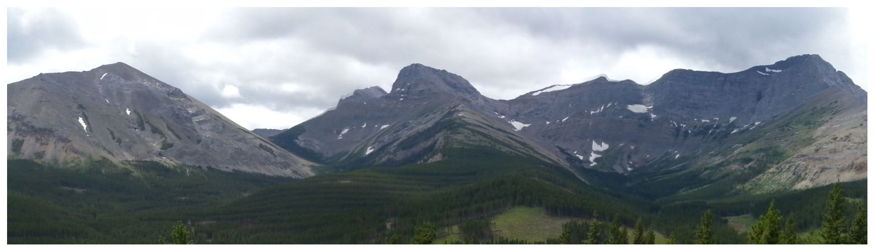
Figure 2Star East (left) and Star West (right) sub-watersheds. The Star East alpine area is more constrained and smaller than the Star West alpine area. Both sub-watersheds have steep headwalls with talus slopes in the alpine zone.
Two historical streamflow gauging sites exist in each sub-watershed – a lower site (Star West Lower – SWL; Star East Lower – SEL) near the confluence of the two sub-watersheds (1540 m a.s.l.) and an upper site (Star West Upper – SWU; Star East Upper – SEU) located at approximately 1690 m a.s.l. in the sub-alpine transition zone (Fig. 1). The sub-alpine and upper montane zones are dominated by sub-alpine fir (Abies lasiocarpa) and Engelmann spruce (Picea engelmannii) above forests dominated by lodgepole pine (Pinus contorta) at lower elevations (Dixon et al., 2014; Silins et al., 2009). Vegetation in upper and lower watersheds (Fig. 1) are distinguished by a transition between higher-elevation alpine heath/shrub vegetation and sub-alpine fir-dominated forests in the upper watersheds and lodgepole-pine-dominated forest in the lower watersheds.
3.1 Stream water chemistry
Stream water samples were collected from the four streamflow gauging stations (SEL, SEU, SWL, and SWU; Fig. 1) every 2 weeks, from April to October in 2014 and 2015, to capture the full range of streamflow chemistry over the hydrologically active period. Plastic bottles of 1 L in volume were triple rinsed prior to sample collection. Samples were analyzed for major cations and anions (Na+, Mg2+, Ca2+, K+, Cl−, and ) and silica (Si as SiO2) in the Biogeochemical Analytical Service Laboratory (University of Alberta). An inductively coupled plasma–optical emission spectrometer (iCAP 6300; Thermo Fisher Scientific) was used to measure Na+, Mg2+, Ca2+, and K+ with an analytical precision of 1.9 %, 3.0 %, 1.9 %, and 2.4 %, respectively. An ion chromatograph (Dionex DX 600 and Dionex ICS-2500) was used to measure Cl− and , with an analytical precision of 2.4 % and 3.1 %. Flow injection analysis (Lachat QuikChem 8500 FIA automated ion analyzer) was used to measure Si, with an analytical precision of 3.4 %.
Continuous stream discharge was estimated from stage–discharge relationships developed at each gauging station. Stage was measured at a 10 min interval, using a bubbler system (H-350/355 WaterLOG Series; YSI Inc. and Xylem Inc., Yellow Spring, OH, USA) or a pressure transducer (HOBO U20; Onset Computer Corp.; Bourne, MA, USA). Discharge measurements were taken 12–18 times with a velocimeter (SonTek and Xylem Inc.; San Diego, CA, USA) from April to October at each site in 2014 and 2015.
3.2 Source water chemistry
Stream water sources were a priori hypothesized to consist of rain, snowmelt, soil water, hillslope groundwater, till groundwater, and bedrock groundwater (seeps used as a proxy for till and bedrock groundwater), based on field observations and inferences made from research conducted in this watershed since 2004 (Silins et al., 2016). All source water samples were collected in triple-rinsed (with source water) 50 mL plastic vials and analyzed with the same methods as the stream water samples to support application of end-member mixing analysis. Source water collection and sampling methods are detailed below.
3.2.1 Rainfall and snowmelt
Rain samples were collected in clean buckets rinsed with deionized water. Buckets were placed in open areas throughout the watershed or in the nearby townsite (Coleman, AB; within approximately 8 km of the Star Creek watershed) after a rainstorm began. Locations were chosen opportunistically, depending on storm timing and site access. Samples were collected at the end of the day or once there was enough water in the bucket to sample to prevent changes in chemical composition due to dry deposition of dust or evaporation. A total of five, four, and three samples were collected throughout the summers of 2013, 2014, and 2015, respectively. The difficulty in capturing large convective storms and the large frequency of storms of less than 5 mm (Williams et al., 2019) prevented the collection of more rainfall samples.
A total of nine snowmelt samples were collected from the sub-alpine regions of Star Creek and two from North York Creek (an adjacent watershed; Fig. 1) throughout spring and early summer in 2014. Three additional samples were collected in spring 2015, but mid-winter melt of snowpacks hindered the collection of more snowmelt samples. Eavestroughs, 3 m in length, were installed perpendicular to the stream, with a small overhang off the edge of the hillslope in Star Creek and North York Creek watersheds in the fall prior to snow accumulation. Samples were collected directly from snowmelt troughs and snow bridges with clearly visible melt. Snowmelt was sampled, instead of the snowpack, to better reflect the meltwater signature during the snowmelt period (Johannessen and Henriksen, 1978; Williams et al., 2009). The timing of sample collection was based on access to backcountry sites, and samples were taken opportunistically when crews were in the area and were able to observe active snowmelt.
3.2.2 Soil water
Suction lysimeters were installed between 30–60 cm depth using a hand auger in two locations near the toe of the hillslope in each sub-watershed in early spring 2014 (2015 for SEU; Fig. 1). Suction lysimeters consisted of a 0.5 Bar ceramic cup and 38.1 mm PVC pipe to ensure that ample water was collected for chemical analyses. Water from the suction lysimeter was sampled using a hand pump every 2 weeks between April and October in 2014 and 2015. Suction lysimeters were pumped dry following sampling, and pressure was applied. Thus, soil water was composed of water that was able to pass through the ceramic cup over the 2-week period until the lysimeter was at equilibrium pressure with the surrounding soil. Shallow depths were targeted with the intention to collect the unsaturated soil water above the saturated zone in the hillslope, which was sampled separately.
3.2.3 Hillslope groundwater
Hillslope wells were installed with a shovel or hand auger to depth of refusal or maximum auger depth (1.5 m) near the hydrometric gauging stations at SEL, SEU, SWL, and SWU (Fig. 1). A site was added at SEU at the end of the summer in 2014, whereas the other sites were established during summer 2013. Wells were installed in three locations at each site, namely riparian, toe slope, and hillslope positions, to determine the full range in hillslope groundwater. Well depths ranged between 0.5 m (riparian wells) and 1.6 m. Wells were purged, using a hand pump, prior to sampling. Samples were collected approximately every 2 weeks, as available, between April and October in 2014 and 2015. Samples from the upper hillslope wells were generally only obtained during the snowmelt or high flow period; these wells were often dry during late summer. Riparian and toe slope wells contained water for all or most of the year, respectively. Water table depths were monitored with capacitance loggers (Odyssey, Dataflow Systems Ltd., New Zealand) at 10 min intervals to identify the timing of shallow groundwater table responses to infer potential periods when hillslope–stream connectivity occurred.
3.2.4 Groundwater seeps
At the onset of this research, a lack of access to backcountry sites restricted the installation of deep bedrock or till groundwater wells in upper sub-watersheds. Rather, groundwater seeps were used to characterize the possible range in groundwater signatures (both bedrock and till groundwater) within Star Creek. Seeps are defined here as areas of visible water seeping from hillslopes proximal to the stream or from small wetland areas further from the stream that form small tributaries or rivulets that flow into the stream. The east and west forks were initially surveyed from the confluence with the main stem to the stream origins in the alpine area in July 2013. A total of 25 visible seeps were identified, which ranged in duration and magnitude of their contributions to streamflow. Some seeps were only active during the snowmelt season and recession period, reflecting streamflow dynamics. Other seeps were relatively stable throughout the entire snow-free period or throughout the winter baseflow period. Samples were collected during the following three flow conditions: high flow (May/June), recession flow (mid-July), and baseflow (early September prior to fall rains), in both 2014 and 2015. This sampling campaign required more resources than for other sources; as a result, sampling was completed only three times a year during the hydrologically important extreme flow conditions rather than every two weeks from April to October as for other sources. Water temperature and electrical conductivity were measured with a handheld multimeter (YSI85; YSI Inc. and Xylem Inc.; Yellow Spring, OH, USA) during sample collection to aid in differentiating between deep bedrock groundwater, till groundwater, and hillslope groundwater.
3.2.5 Bedrock and till groundwater
Preliminary end-member mixing analysis showed that a water source was missing from those initially collected (above), highlighting the need to characterize deeper groundwater. Due to monetary and access limitations, a single borehole was drilled to 12 m depth (15.2 cm in diameter) in the topographic ridge between SEL and SWL (approx. 500 m upstream from gauging sites) in October 2015 (Fig. 1). Two wells were installed in the borehole, one well in a water-baring formation in the bedrock at 11 m depth and a second well in the glacial till deposits at 4.5 m depth, to characterize the differences in bedrock and till groundwater chemistry. Both wells had screens that were 1.5 m in length. Sand was used to backfill the borehole around the screened section of the bedrock groundwater well and was capped with bentonite clay. Local material removed during drilling was used to backfill the borehole up to the till layer. The same method of back filling (sand, bentonite clay, and local material) was used for the till groundwater well. Bedrock and till wells were sampled every 2 to 4 weeks from April to October in 2016 and 2017. Water in the till well was purged until dry prior to sampling. Water in the bedrock well was purged for 2–5 min prior to sampling because the recharge rate was faster than the pump rate. Water table depth and temperature were measured continuously with pressure transducers (HOBO U20; Onset Computer Corp., Bourne, MA, USA) at 10 min intervals.
High concentrations of Na+, Cl−, and in till groundwater (Fig. 3) and large variability between years suggested that the till groundwater well was likely contaminated by the bentonite clay used to backfill and seal between layers (Remenda and van der Kamp, 1997). Slow recharge rates (and, therefore, low hydraulic conductivity) of glacial till prevented the removal of three pipe volumes when sampling, and the corresponding low hydraulic conductivity resulted in little flushing of bentonite contaminants. Faster recharge rates (and, therefore, higher hydraulic conductivity) of the bedrock groundwater would aid in better flushing of bentonite contaminants, which would reduce the effects on bedrock groundwater chemistry (Remenda and van der Kamp, 1997). As a result, the till groundwater samples were not included in the analyses herein; however, water table depths and water temperature dynamics could still be used to understand the differences between till and bedrock groundwater responses and their roles in runoff generation.
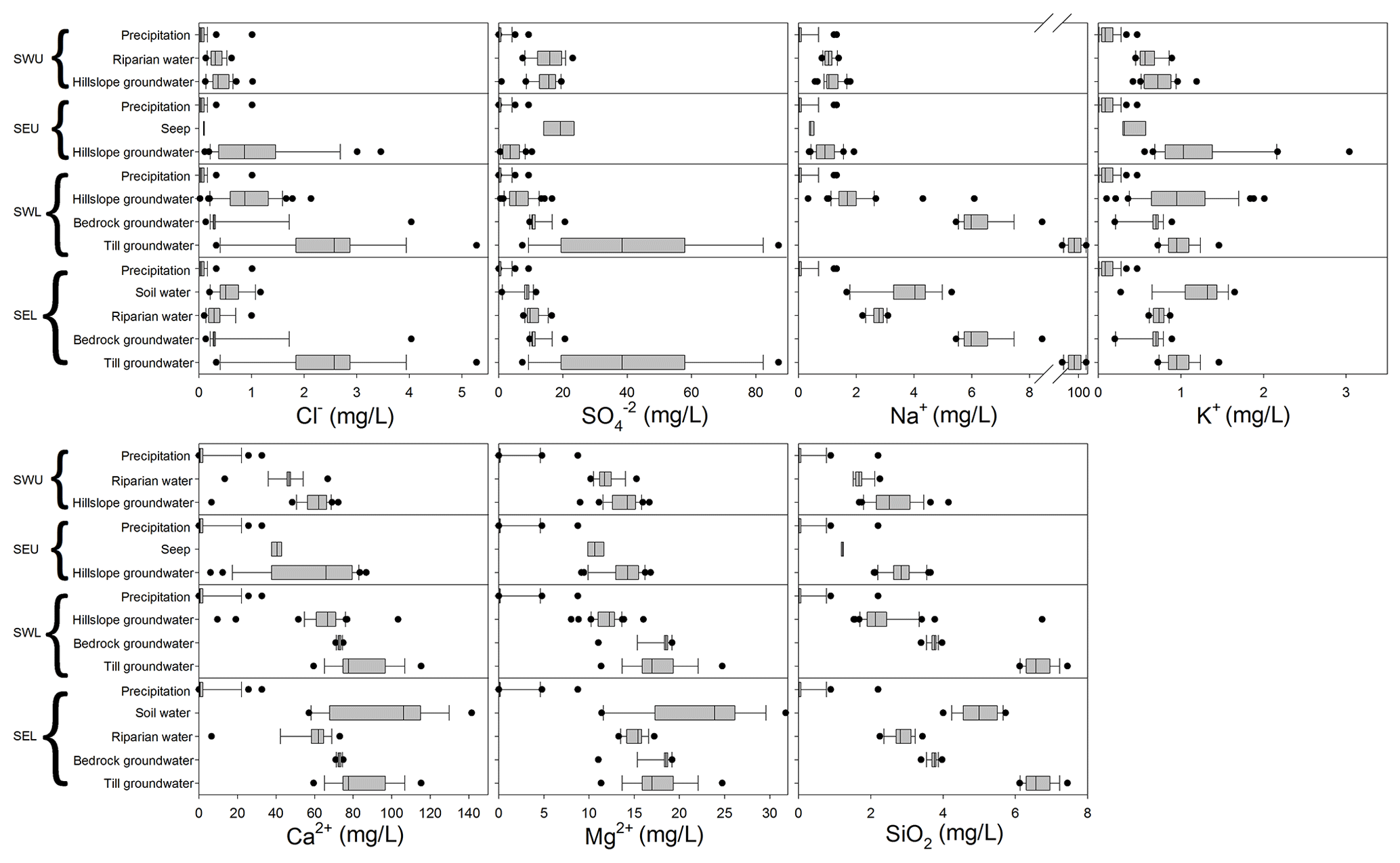
Figure 3Box plots for Star West Upper (SWU), Star East Upper (SEU), Star West Lower (SWL), and Star East Lower (SEL) showing the ranges in chemistry for potential sources.
End-member mixing analysis (EMMA) was used to visualize multivariate source water and stream chemistry by reducing the dimensionality of the data with principal component analysis (PCA; Christophersen and Hooper, 1992). In addition, there were multiple subjective decisions required prior to EMMA, such as choosing tracers/ions and defining sources. Bivariate plots and tracer variability ratio (TVR) were used to determine if tracers were appropriate to use in the analysis. First, a matrix of bivariate plots of stream chemistry data (ion concentrations), used most commonly in geographical hydrograph separations, was used to determine if ions were conservative in nature (Hooper, 2003). A linear relationship between tracers can be interpreted as a sign of conservative relationships. Second, TVR, used most commonly in sediment source apportionment studies, was used to determine if the difference in ion concentrations between groups was larger than the variation within a source group (Pulley et al., 2015). TVR was calculated using the following equation for each tracer and compared between each source group pair:
where is the maximum median tracer concentration of either source group, is the minimum median tracer concentration of either source group, and CV is the coefficient of variation (Pulley et al., 2015; Pulley and Collins, 2018). TVR should be greater than two to be considered appropriate for use in mixing calculations (Pulley and Collins, 2018), although, depending on the data set in question, a greater threshold may be adopted to make the tracer selection more stringent and to help reduce the numbers of tracers included in further data processing.
Box and whisker plots and linear discriminant analysis (LDA) were used to remove the subjectivity of the defining sources (Ali et al., 2010; Pulley and Collins, 2018). Box and whisker plots were used as a visual means of discriminating between sources. LDA was then used to determine if the combined sources exhibited sufficiently robust statistical separation (Pulley and Collins, 2018). LDA optimizes separation between the centroid of group clusters by partitioning the variation across each tracer and weighing that variation into two axes (reducing the dimensionality). Other statistical classification methods, such as hierarchical clustering or k-means clustering, were not appropriate because source categories were known a priori. The data were processed in R (R Core Team, 2014), using the lda function in the MASS package (Venables and Ripley, 2002) to reduce dimensionality and assess the separation visually and the klaR (stepwise function; Weihs et al., 2005) package to model the data and determine the ability to separate groups statistically. The stepwise function models the data while removing individual tracers iteratively. The backwards direction was used in an attempt to maintain the most tracers with the lda method and ability to separate criterion.
After the sources were characterized, the stream water was processed using principal component analysis (PCA; prcomp function in R; R Core Team, 2014) as a method of dimensionality reduction to create a two-dimensional (2D) mixing space (Christophersen and Hooper, 1992). Stream water was standardized (subtracting the mean and dividing by the standard deviation for each sampling point) for each tracer, to create equal variance between chemical components, and used to create a correlation matrix. PCA was conducted on the correlation matrix to calculate eigenvectors and eigenvalues. Standardized stream water was then projected into the end member mixing space by multiplying by eigenvectors. Ideally, two principal components (PCs) explained most of the variation in the data and were used to generate a 2D mixing space, which corresponds to three sources in EMMA (Hooper, 2003). Other studies have used the rule of one to determine how many dimensions, and therefore sources, should be used to create the mixing space (Ali et al., 2010; Barthold et al., 2011). For this study, the mixing space was set to two dimensions for ease of visualization but used all appropriate sources, as presented by Inamdar et al. (2013), to provide a full description of potential source contributions. Source water was then standardized, using stream water means and standard deviations for each ion, and projected into the 2D mixing space as defined by the stream water (Christophersen and Hooper, 1992; Hooper, 2003). Stream water sources should create an outer boundary or polygon around all stream water samples if all sources were correctly identified and adequately sampled.
5.1 Tracer and source water group selection
Bivariate plots were created, and TVR was calculated to determine which tracers were appropriate for use in EMMA. Pearson correlation coefficients were calculated between all stream bivariate plots for stream water at each sub-watershed (Fig. 4). These showed that all tracers exhibited acceptable linear trends with at least one other tracer (Pearson's r>0.5; p<0.05) and were thereby likely conservative in nature. TVR for almost all tracers at all sites were below two, with the exception of precipitation group comparisons, which suggested that the within-group variation exceeded the between-group variation for all subsurface sources. Greater variation within source groups compared to between source groups violates assumption 3 for EMMA (source water does not change) and was considered unacceptable. As a result, rather than calculating the mixing ratios or percent contribution of sources to stream water on the basis of an unmixing routine in EMMA, trends in stream water distribution were described in relation to source water dynamics and runoff processes.
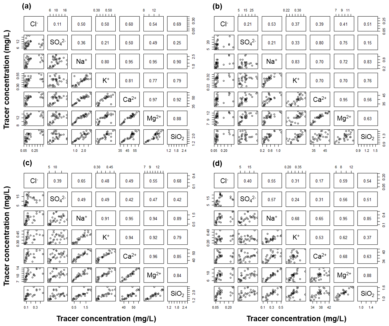
Figure 4Bivariate plots of stream water chemistry at (a) Star East Lower, (b) Star East Upper, (c) Star West Lower, and (d) Star West Upper. Top half of plots represents the Pearson's correlation coefficient (r) for the linear relationship between each solute.
The a priori classification of water sources was rain, snowmelt, soil water, hillslope groundwater, till groundwater, and bedrock groundwater; however, not all sites conformed to these categories. Box and whisker plots showed that the distribution of rain and snowmelt was too similar for them to be considered as separate groups. Although riparian water mixes with stream water and should be chemically different from hillslope water as a source, soil water, toe slope water, and upper hillslope water were grouped with riparian water for most sites because the distribution of these samples were too similar to be considered separate sources. The exception was SEL and SWU, in which riparian water was considered as a separate source. Final source water groups are described below for each sub-watershed. LDA plots indicated that LD1 and LD2 explained 88.5 % and 11.5 %, 95.3 % and 4.7 %, 81.1 % and 15.5 %, and 77.6 % and 22.4 % of the variance of the centroids for SWL, SWU, SEL, and SEU sites, respectively. Stepwise analyses were also used in attempt to reduce the redundancy of the tracers and to ensure that samples were well separated; on this basis, 99.7 %, 91 %, 98.6 %, and 99.9 % of samples were well separated in SWL, SWU, SEL, and SEU, respectively. In all sites, all tracers were retained to maximize the ability to distinguish between the source groups. Overall, these results support the conclusion that there was good separation between the source water groups as they were recategorized for the individual sites.
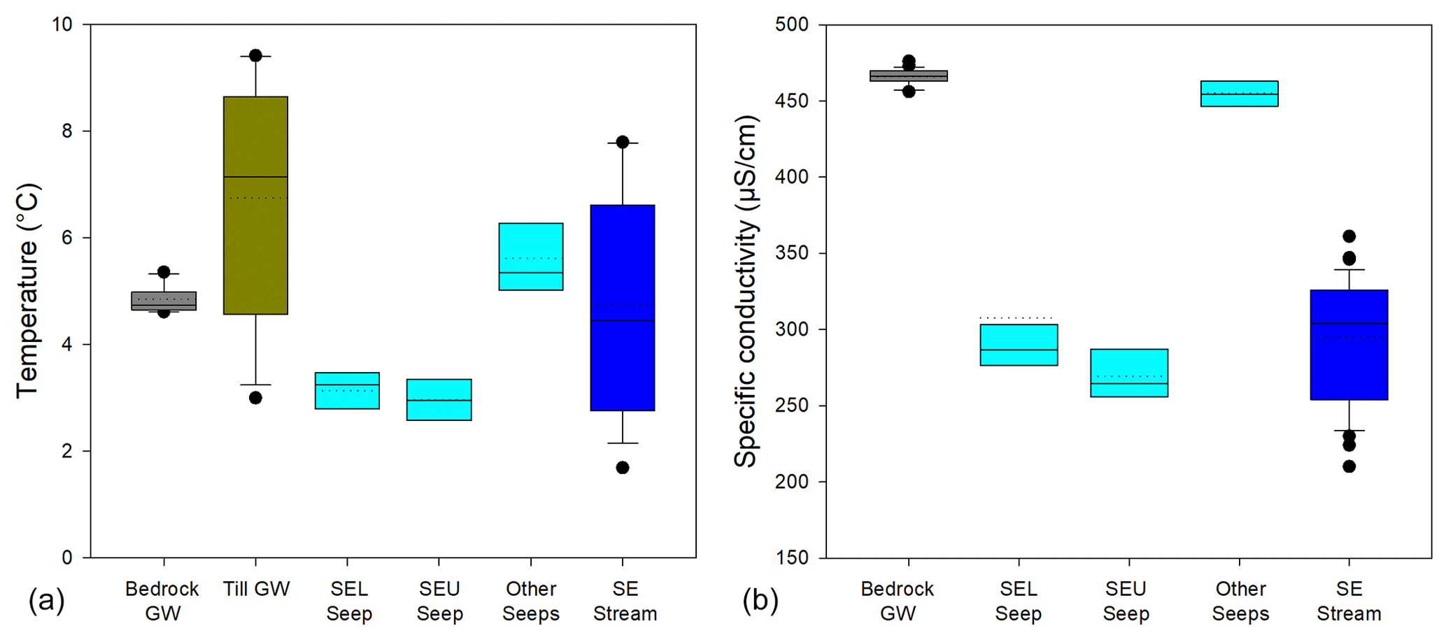
Figure 5Box and whisker plot of groundwater, seep, and stream water temperature (a) and specific conductivity (b). Solid line indicates the median, and the dashed line indicates the mean. The box indicates the 25th and 75th percentiles, the whiskers indicate the 90th percentiles, and the circles indicate points within the 5th and 95th percentiles. Other seeps are shown here as an example of the temperature and specific conductivity in many of the other seeps that were identified in the watershed but not used in the PCA biplots.
At the outset of this research, groundwater seeps were sampled in lieu of bedrock and till groundwater wells to characterize the variability in the chemical signature of groundwater throughout Star Creek. Most ion concentrations of the groundwater seeps were not chemically distinct because they were generally similar to stream water or hillslope groundwater in the PCA analyses (data not shown). However, the water temperature of groundwater seeps from spring to fall revealed that some seeps were consistently cool while others had larger fluctuations in temperature. This suggests that some seeps were potentially groundwater fed and others were fed by shallow subsurface water, respectively. For example, in SEL, the temperature of a groundwater seep ranged between 2.2 and 3.7 ∘C throughout the summer (Fig. 5), which is indicative of a bedrock groundwater source because the temperature range was muted and was largely not influenced by radiative warming (Taniguchi, 1993). In SEU, the temperature of a groundwater seep ranged from 2.5 to 3.5 ∘C (Fig. 5), also indicating a bedrock groundwater source. Temperatures in the till groundwater well ranged between 2.7 and 9.7 ∘C, displaying some radiative heating and cooling, whereas the bedrock groundwater ranged between 5.1 and 5.8 ∘C, displaying little radiative effects (Fig. 5). The groundwater seeps mentioned above had low variability, like bedrock groundwater, but were cooler, suggesting potentially deeper bedrock groundwater sources than in the well. Temperatures of some other groundwater seeps were more similar to bedrock groundwater although more variable, ranging from 3.6 to 5.4 ∘C (data not shown), while others were more similar to till groundwater, ranging from 4.8 to 7.1 ∘C (Fig. 5). The corresponding specific conductivity measurements add further complexity to these patterns. The cool, temporally more stable seeps had low conductivity from April to September, which was not reflective of the specific conductivity in the bedrock groundwater well. Rather, the other seeps with greater variability in temperatures had high specific conductivity, which is more consistent with the bedrock groundwater wells (Fig. 5). Unfortunately, the till-well-specific conductivity could not be used due to the contamination mentioned above, so it was unclear if the till groundwater had similar specific conductivity.
5.2 Source water characterization
5.2.1 Star West source water
Water sources for the SWL sub-watershed were grouped as precipitation (rain and snow), hillslope groundwater (soil water, riparian water, and toe slope water), and bedrock groundwater and plotted in PCA mixing space (Fig. 6). PC1 was mainly driven by cations, and PC2 was driven by anions (Table 1). Minimal variation in chemistry across all precipitation samples (standard deviation (SD) of 2.4 and 1.1 for PC1 and PC2, respectively) and overlap of snow and rain samples in the mixing space confirmed that it was appropriate to aggregate all samples (snow and rain) taken across all sites (Star Creek, York Creek, and Coleman). Hillslope groundwater exhibited greater chemical variation across samples (SD of 3.8 and 2.0 for PC1 and PC2, respectively) compared to bedrock groundwater (SD of 2.9 and 4.8 for PC1 and PC2, respectively), but no clear temporal pattern was observed. Bedrock groundwater chemistry showed slight temporal variation, with more positive values in PC2 in the spring than in the fall.
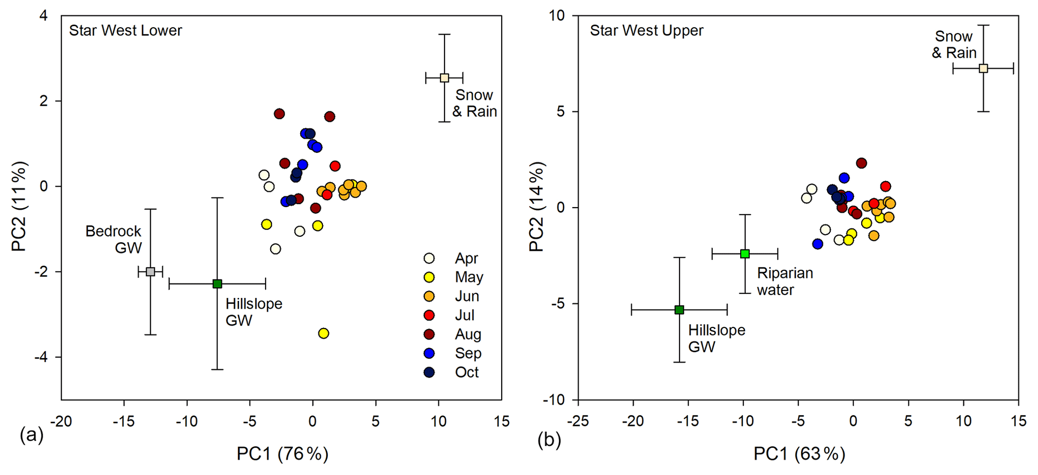
Figure 6The first two principal components (PCs) of variation in stream water chemistry in Star West Lower (a) and Star West Upper (b) from April to October (values in parentheses indicate the percent of variation explained by each PC). Square symbols indicate the mean chemical composition (±1 SD – standard deviation) of stream water sources for each sub-watershed.
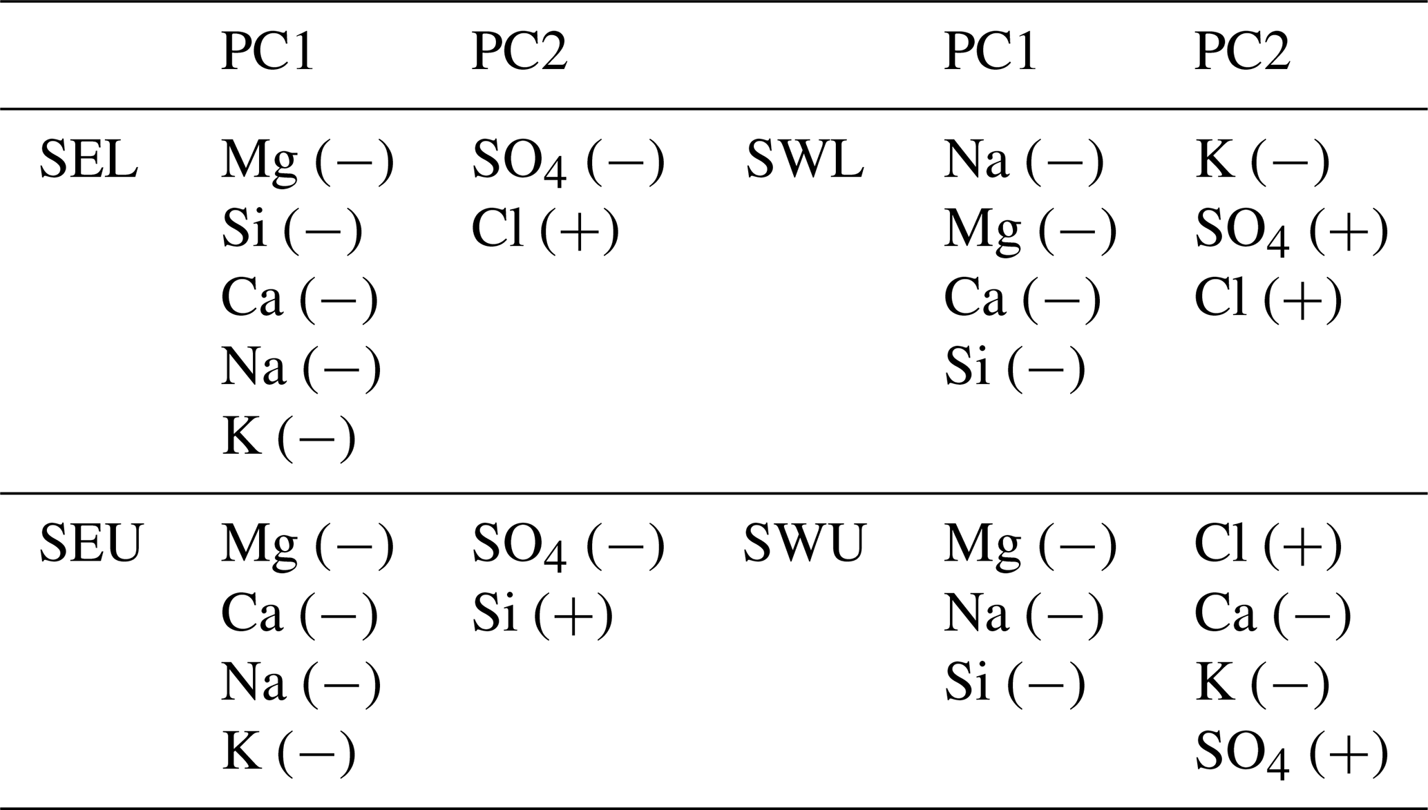
Table 1Ions that explained the most variation in PC1 and PC2 for each sub-watershed in Star Creek.
Water sources for the SWU sub-watershed were similarly grouped as precipitation (rain and snow) and hillslope groundwater (soil water, toe slope water, and upper hillslope water), but here riparian water displayed a greater difference from hillslope groundwater and was considered as a separate source (Fig. 6). Bedrock groundwater samples were collected from a lower elevation in the watershed and may not be representative of higher-elevation groundwater chemical composition; therefore, they were excluded from the analysis for the upper sites. Furthermore, there were only two seeps identified in the upper watershed, but the temperature and chemical composition of these seeps were not reflective of bedrock groundwater. While this did not exclude bedrock groundwater contributions to streamflow in the upper regions of the watershed, it showed the chemical composition of the bedrock well, and the two seeps may not have been representative of the bedrock groundwater chemistry in the Star West Upper sub-watershed. Precipitation clustered tightly in one location, except for four snow samples and one rain sample, which increased the SD for precipitation (SD of 2.7 and 2.3 for PC1 and PC2, respectively). All sources showed similar variation in precipitation; hillslope groundwater had a SD of 4.3 and 2.7 for PC1 and PC2, respectively, and riparian water had a SD of 3.0 and 2.0 for PC1 and PC2, respectively. A temporal pattern was observed for hillslope water in which hillslope water became less like precipitation from spring to fall (Fig. 7). Temporal variation was also observed across months for riparian water and in which concentrations increased from spring to fall (Fig. 7).
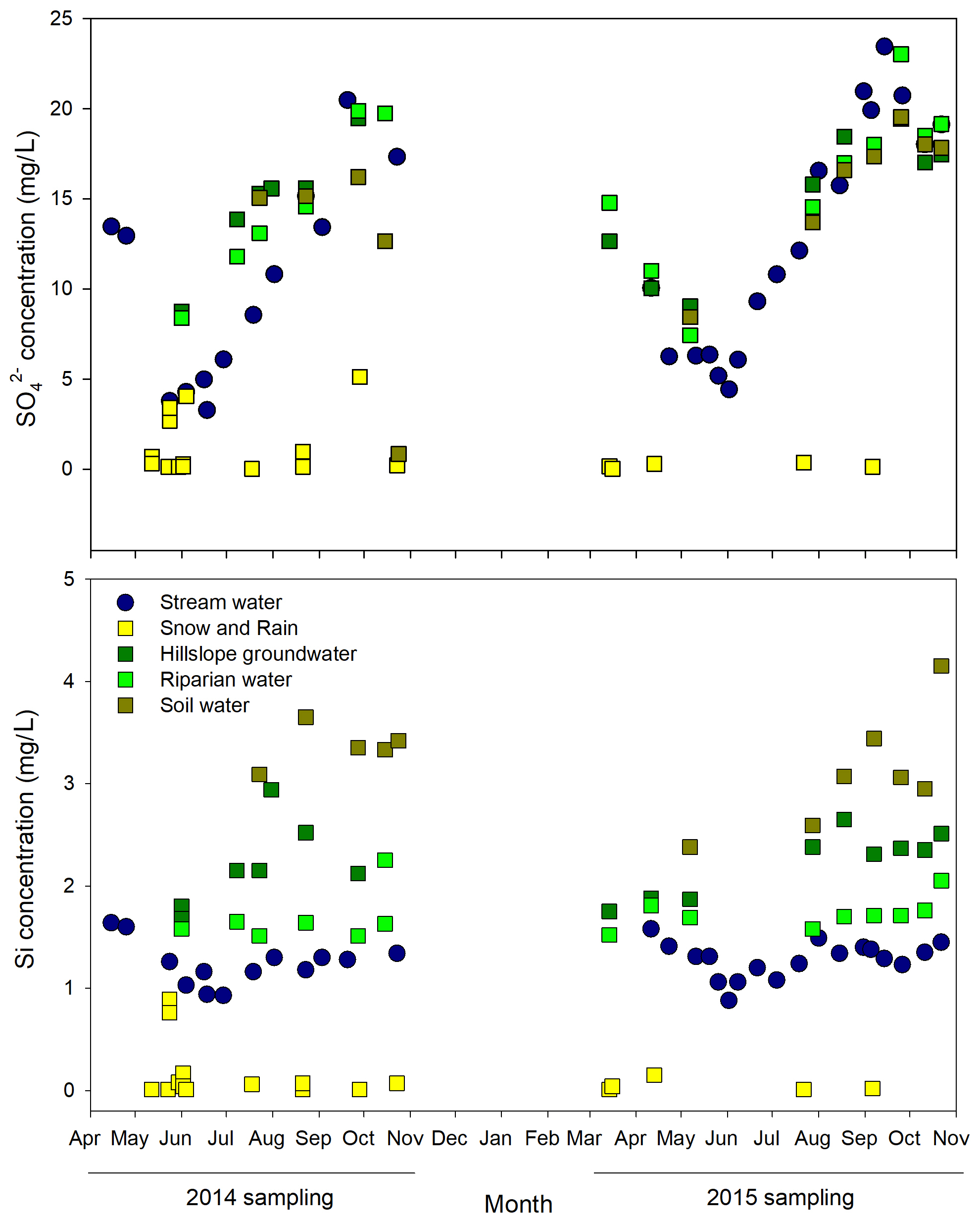
Figure 7Time series of Si and concentration in Star West Upper stream and source water in 2014 and 2015.
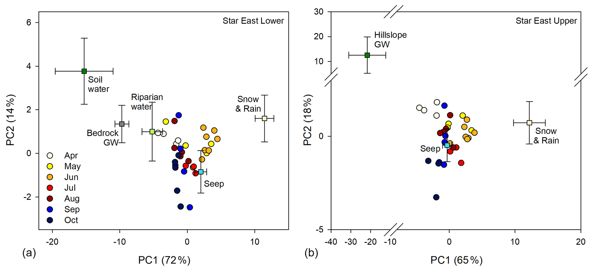
Figure 8The first two principal components of variation in stream water chemistry in Star East Lower (a) and Star East Upper (b) from April to October (values in parentheses indicate the percent variation explained by each PC). Square symbols indicate the mean chemical composition (±1 SD – standard deviation) of stream water sources for each sub-watershed.
5.2.2 Star East source water
Water sources for the SEL sub-watershed were grouped as precipitation (snow and rain), soil water, riparian water, groundwater seep, and bedrock groundwater (Fig. 8). Precipitation (SD of 1.4 and 1.1 for PC1 and PC2, respectively) and bedrock sources (SD of 1.0 and 0.9 for PC1 and PC2, respectively) were the same as those used in SWL. Hillslope groundwater samples were initially grouped together as a single source, but high standard deviations and clustering within the group suggested the separation of riparian water (SD of 1.0 and 1.5 for PC1 and PC2, respectively) and soil water (SD of 4.3 and 1.5 for PC1 and PC2, respectively) into individual sources. Soil water was most different from stream water and varied from spring to fall (increased Ca2+ and Mg2+ concentrations; Fig. 9). Riparian water was most similar to stream water and did not vary over the season. A single groundwater seep that was chemically similar to stream water, but for which temperatures were consistently cool, was retained to aid in the explanation of stream water dynamics (Fig. 8).
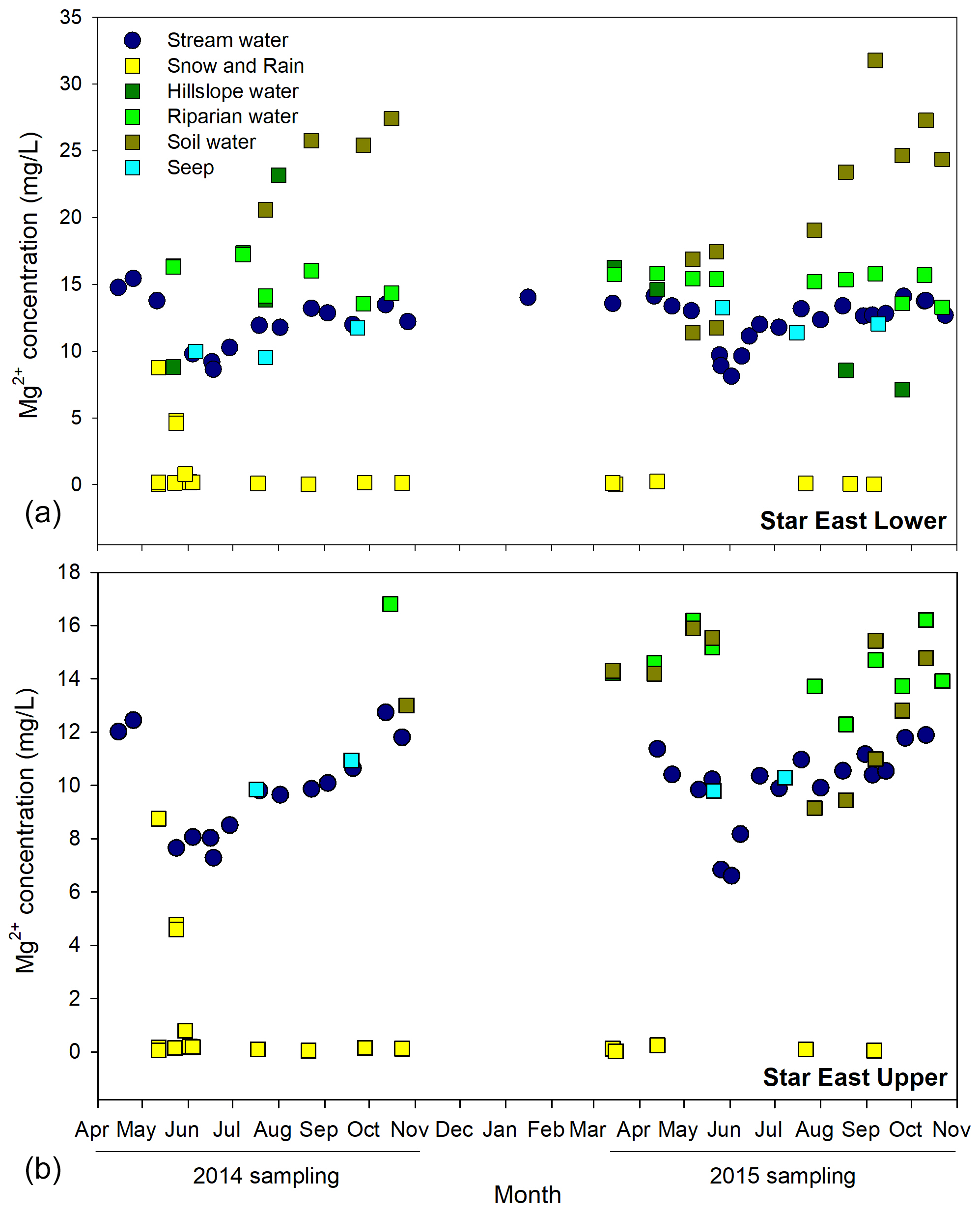
Figure 9Time series of Mg2+ concentration for Star East Lower (a) and Star East Upper (b) stream and source water in 2014 and 2015.
Water sources for the SEU sub-watershed were grouped as precipitation (rain and snow), hillslope groundwater (soil water, riparian water, and toe slope water), and groundwater seep (Fig. 8). Precipitation displayed little variation (SD of 2.4 and 1.1 for PC1 and PC2, respectively). Large variation was observed for hillslope groundwater (SD of 9.3 and 7.3 for PC1 and PC2, respectively). Toe slope water and riparian water had some chemical dissimilarities but were not different enough from each other, or soil water, to be considered as different groups. Some temporal variability was observed in riparian water compared to SEL; however, soil water had much larger temporal variability than riparian water (Fig. 9). A single groundwater seep was identified in SEU. The seep was chemically similar to stream water but temperatures were consistently cool and indicative of a deep groundwater source, so it was retained to aid in the explanation of stream water dynamics (Figs. 8 and 9).
Table 2Streamflow and precipitation metrics for 2014 and 2015 water years.
* Standard deviation in parentheses.
5.3 Stream water characterization
Stream water chemistry for all four sites showed high temporal variation throughout the months of open-water flow (April–October) but little variation between years. As a result, the temporal pattern of stream water was characterized for each site, in general, for 2014 and 2015 combined. Furthermore, due to the lack of source water samples during winter months, the temporal pattern of stream water was characterized from April to October, which represents the most dynamic hydrologic period from the beginning of snowmelt through to the start of the next year's snow accumulation period. Hydrologic characteristics of the 2014 and 2015 water years are indicated in Table 2.
5.3.1 Star West stream water
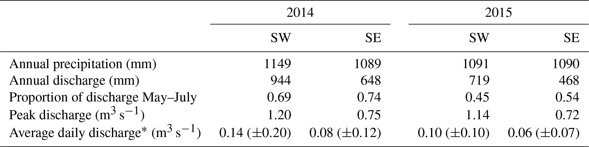
The first two principal components (PCs) from the PCA analysis explained 87 % and 77 % of the variation in stream water chemistry in SWL and SWU streams, respectively. Temporal variation in stream water chemistry was constrained within the broader multivariate mixing space created by the variation in source water chemistry but not within the more constrained mixing space of the mean composition (±1 SD) of these sources (Fig. 6). In April, stream water was most similar to the hillslope groundwater (and riparian water in SWU). Stream water transitioned through May to become the most similar to precipitation source water in June (and July in SWU). In SWL, stream water was slightly more similar to hillslope groundwater and bedrock groundwater in July. In August–October, stream water chemistry was more variable and was similar to precipitation and hillslope and bedrock groundwater. The temporal pattern associated with variation in stream water chemistry through the fall was perpendicular to the direction of the bedrock temporal pattern, suggesting that hillslope groundwater (soil water, toe slope water, and riparian water), rather than bedrock groundwater, was driving the variation in stream water chemistry in the fall in SWL. Time series of Ca2+ and show that hillslope groundwater was most similar to stream water (Fig. 10). Stream water in SWU was again more chemically similar to hillslope groundwater and riparian water through August–October, but stream water chemistry differed slightly from its chemical composition in the early summer months. Riparian water chemistry had a similar temporal shift from April to October as stream water chemistry, whereas hillslope groundwater and soil water had greater temporal variation (Fig. 7). Furthermore, water table depth in the hillslope well indicates that the upper hillslope is largely disconnected from the stream in the fall in both SWL and SWU (Fig. 11), so it is more likely that the riparian area is contributing flow to the stream in the fall.
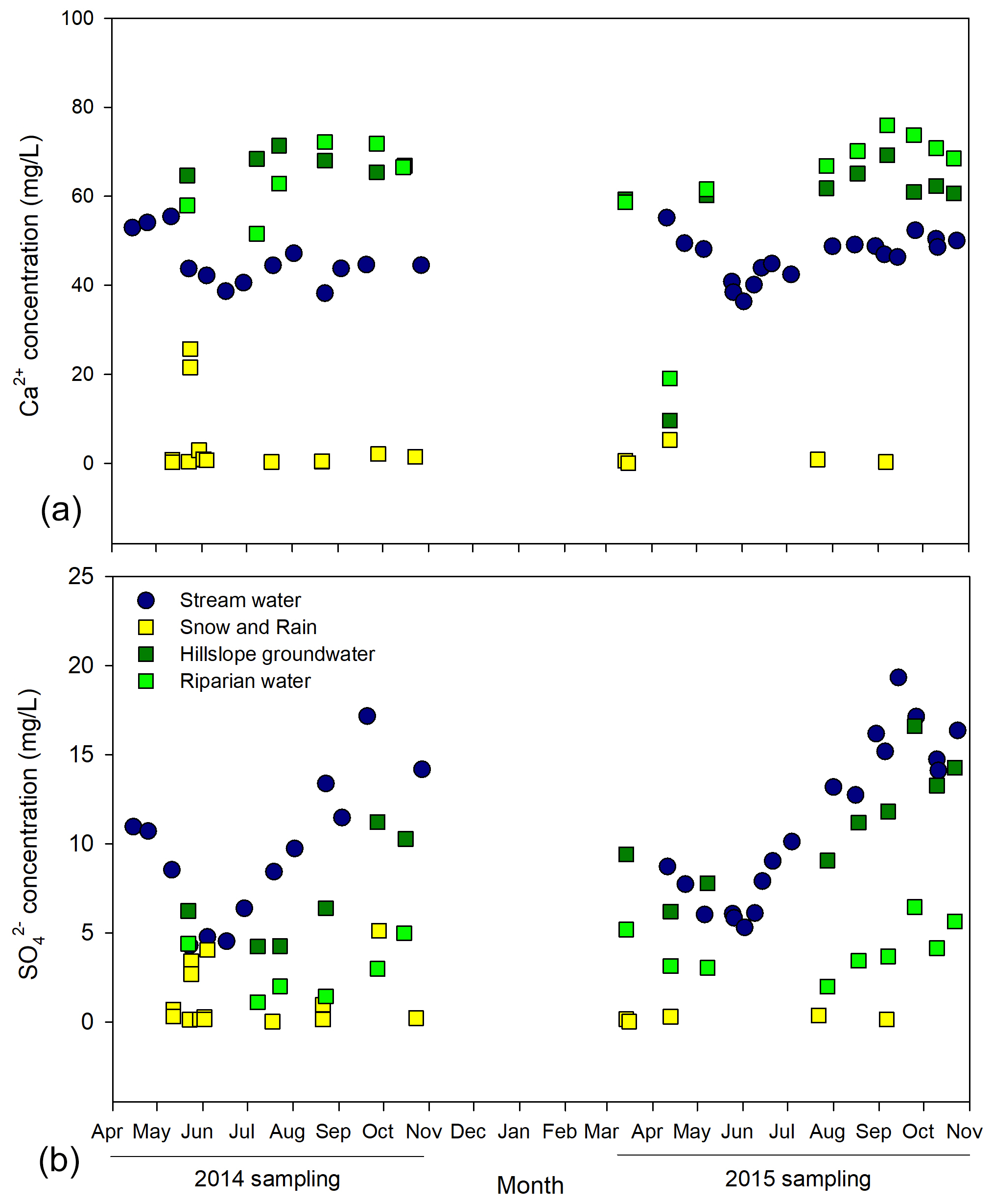
Figure 10Time series of Ca2+ and concentration in Star West Lower stream and source water in 2014 and 2015.
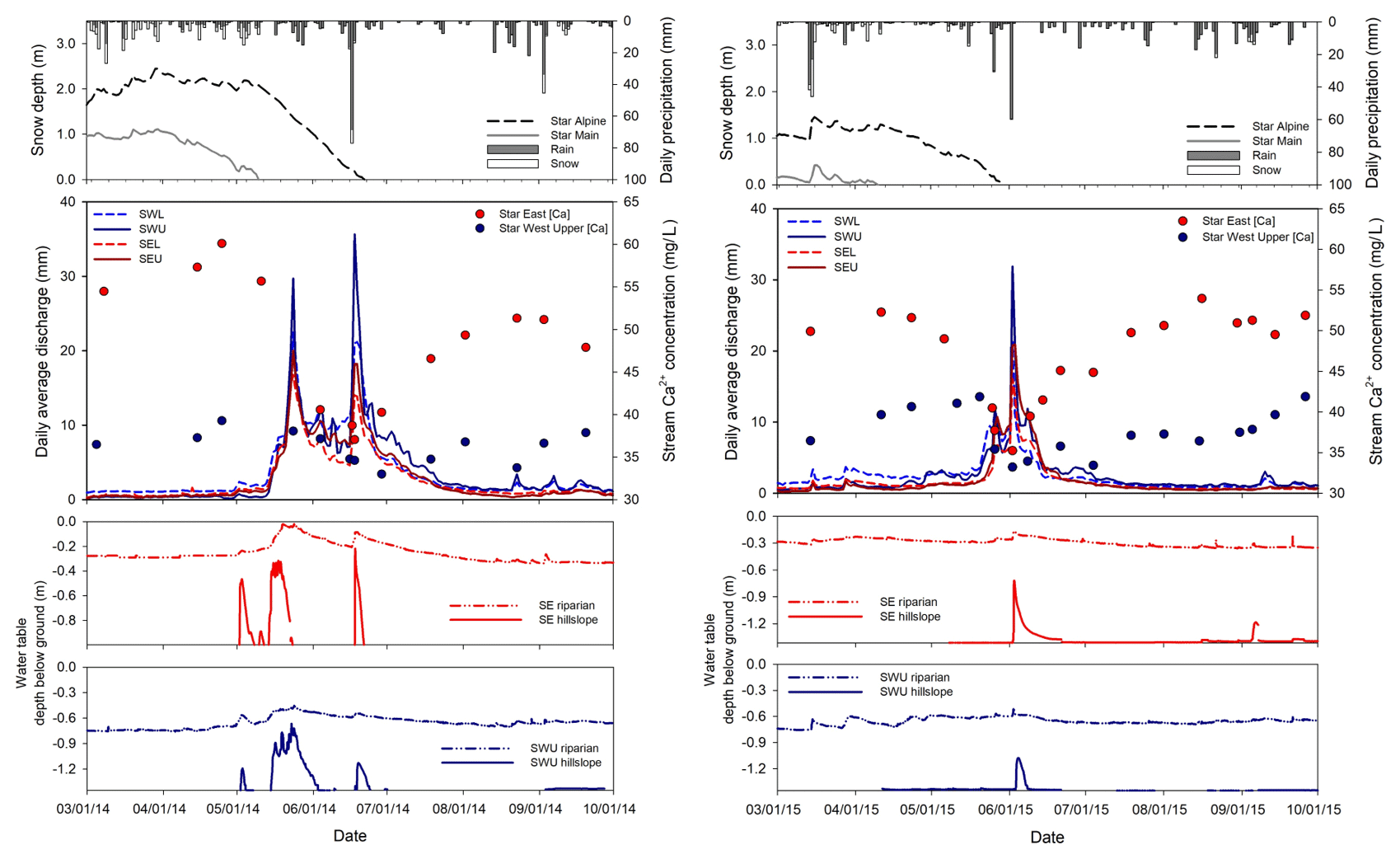
Figure 11Observed inputs (snow depth and daily precipitation – estimated snow and rain proportions) and responses (stream discharge, stream Ca2+ concentration, and shallow groundwater wells – hillslope and riparian) for Star Creek sub-watersheds in 2014 (left) and 2015 (right). Precipitation phase was separated into snow and rain after Kienzle (2008).
5.3.2 Star East stream water
Temporal patterns of variation in stream water chemistry observed for SEL and SEU were very consistent with each other, again with the exception of the bedrock groundwater well, which was only sampled at a lower elevation site and, therefore, not included in the PCA analysis in SEU. However, seeps that displayed temporal stability in water temperature typically characteristic of deep groundwater (Fig. 5) were used in the analysis for both SEL and SEU. The first two PCs explained 86 % and 83 % of the variation in stream water chemistry in SEL and SEU, respectively (Fig. 8). For both sub-watersheds, temporal variation in stream water chemistry was mostly constrained within the mixing space produced by the variation in source water chemistry, except during September/October when stream water plotted outside this boundary. In April, stream water was most similar to the riparian/hillslope water (or bedrock groundwater for SEL). The chemistry of stream water transitioned through May and was most similar to precipitation in June. In July and August, stream water became dissimilar from precipitation and was once again similar to riparian/hillslope water or bedrock groundwater. In September and October, stream water was less similar to riparian/hillslope water and plotted outside the mixing space of the identified sources. Since stream water was not contained within the boundary created by the source water, it is likely that an additional source was not captured by field sampling. However, the temporal variation in the chemistry of the groundwater seep followed the same pattern as the September/October stream water in both sub-watersheds, suggesting the same source water for the groundwater seep and late fall baseflow (Fig. 8). Consistently cool temperatures of the seep in SEL (2.2–3.7 ∘C) and SEU (2.5–3.5 ∘C) suggest a deeper groundwater source.
Twice monthly stream water and source water samples collected in Star Creek, from April to October in 2014 and 2015, have been used here to conceptualize runoff generation in Alberta's Rocky Mountains. Results from this study allow for a detailed examination of temporal patterns in source water chemistry and a qualitative description of source water contributions to stream water. While our intention was a quantitative estimate of source water contributions to streamflow using an unmixing routine, two of the key assumptions for EMMA, the chemical composition of sources does not change (1) over the timescale considered or (2) with space (Hooper, 2003; Inamdar, 2011), were violated in this data set. Source water chemistry varied greatly across the watersheds. For example, when all hillslope samples from each sub-watershed were projected into the mixing space created by stream water at the watershed outlet (SM), large variability was evident between sites (Fig. 12). While there was some overlap between some sites (SWL and SEU), SWU was clearly different than the other hillslope samples. As a result, source water from within individual sub-watersheds was used to reduce the uncertainty associated with large spatial variability in source water chemistry. However, the variability within sites was also quite large. The CV of source water tracer concentrations was often larger than the CV of the stream water tracer concentrations (there should be little to no variation in source water over time; James and Roulet, 2006; Inamdar, 2011), particularly for K+. The occasions where source water CV was smaller than stream water CV for most ions were for seeps in SEU and SEL, bedrock groundwater in SWL and SEL, and hillslope and riparian water in SWU. Chemical signatures of source water have been shown to vary seasonally and annually (Rademacher et al., 2005) and spatially across sub-watersheds in southern Quebec, Canada (James and Roulet, 2006). As a result, James and Roulet (2006) suggested that only source water from within individual sub-watersheds of interest should be used in unmixing calculations. Inamdar et al. (2013) further argued that mixing proportions should not be calculated because multiple assumptions are often violated and can lead to significant errors in unmixing proportions. Rather, temporal and spatial variation in stream water and source water should be examined and used to describe or to develop a physically based conceptualization of runoff mechanisms.
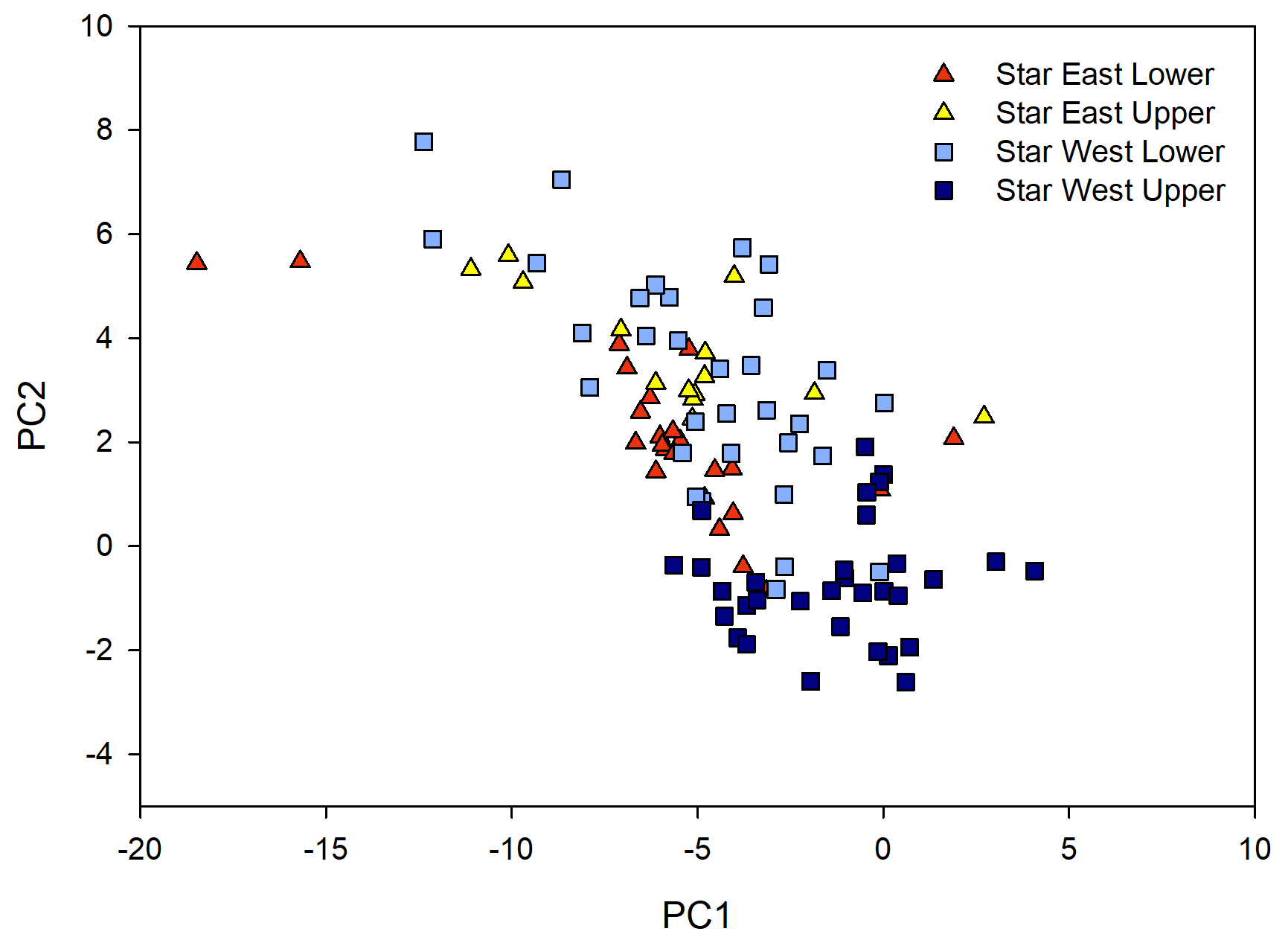
Figure 12Hillslope groundwater from all sub-watershed sites in 2D mixing space, which was derived from a principal component analysis of Star Main (Fig. 1) stream water. PC1 and PC2 represent the first and second principal components.
The inability to run the unmixing routine (stream water fell outside the bounds of the source water) also hindered the use of some tracer selection methods. Other studies have often used the selection criteria presented in Barthold et al. (2011), but the unmixing routine is required for this method. Rather, the TVR and LDA have been presented as effective parameters to subjectively determine if tracers are included in the analysis and if sources are well separated or grouped appropriately, respectively (Pulley et al., 2015, Pulley and Collins, 2018, and others – see the comprehensive review in Collins et al., 2017).
Despite the violation of assumptions, notable temporal trends in source water chemistry were observed in snowmelt, riparian water, hillslope and soil water, and bedrock groundwater and their contributions to stream water can be generalized for all sub-watersheds in Star Creek in a number of ways. The water that was stored in the hillslope over winter (or reacted water) was likely the first to reach the stream in the early spring prior to high flow as snowmelt started to saturate the landscape (Figs. 6 and 7). Temporal patterns in stream water chemistry also showed a spike in concentrations of some ions (e.g., Ca2+ concentration in Fig. 11) in the stream in the early spring, as this reacted water mobilized prior to the onset of the snowmelt freshet. Although three snowmelt samples in 2014 showed similar ionic pulses early in the snowmelt season to those reported in the Colorado Rocky Mountains (Williams et al., 2009), the concentrations were notably less than from all other sources and, thus, not likely an important source of the observed early season increase in stream water concentration of some ions. Rather, the delivery of reacted water to the stream at the onset of snowmelt is likely similar to the flushing mechanism observed in the Turkey Lakes watershed in central Ontario, Canada (Creed and Band, 1998), where high nitrogen concentrations were observed prior to peak streamflow. McGlynn et al. (1999) observed the displacement of old water to the stream at the onset of snowmelt in the Sleepers River research watershed in Vermont, USA, and suggested this was due to a small volume of snowmelt being added to a large storage of water already in the subsurface.
This initial displacement of reacted water was followed by a dilution effect, where large volumes of low-concentration snowmelt mixed with soil water and contributed to streamflow. Snowmelt was the major event that produced a water table response in all hillslope wells and connected the hillslopes to the stream (Fig. 11; Spencer et al., 2019). The initial snowmelt period was also the only time that overland flow was observed at the study site. Other studies have also reported that snowmelt creates a dilution response in the stream (Rademacher et al., 2005; Cowie et al., 2017). Conversely, the opposite has been observed whereby a previously disconnected source was connected to the stream and caused an increase in solute concentrations (McNamara et al., 2005). Although this was the main period of hydrologic connectivity in Star Creek (Fig. 11), we did not observe an increase in stream water ion concentrations associated with newly connected sources. Hillslope groundwater and soil water chemistry should reflect the dilution from snowmelt and the subsequent drying of the hillslope, thereby increasing ion concentrations in the soil water from spring to fall. This corresponding temporal pattern in hillslope groundwater chemistry was observed in SWU (Fig. 7) and for soil water chemistry in SEL and SEU (Fig. 9).
Source water contributions to the stream were more similar within Star East (SEL and SEU) and Star West (SWL and SWU) sub-watersheds than between alpine/sub-alpine (SEU and SWU) and upper montane (SEL and SWL) sub-watersheds. PCA plots for SEL and SEU showed that stream water chemistry was most similar to precipitation in May and June, whereas a dilution effect from snowmelt occurred in June and July in SWL and May to July in SWU. It should be noted that although dilution was observed, stream water was less diluted than snowmelt alone. Snowmelt water interacts with the soil as it moves through the subsurface to the stream, directly influencing the chemical composition of the snowmelt contributions to streams (Sueker et al., 2000). The delayed response in SWL and SWU is consistent with the watershed storage estimates from baseflow recession analysis (Spencer et al., 2019) that suggested that the west fork sub-watersheds had a larger storage capacity than the east fork sub-watersheds. Accordingly, more water would be required to fill the storage before saturation or hydrologic connectivity could occur.
Differences in the east and west forks were also evident in the hysteresis pattern in stream water chemistry from spring to fall. Star West sub-watersheds had a counterclockwise pattern, whereas Star East sub-watersheds had a clockwise pattern. In general, this is an artefact of the PCA analysis driven by the specific ions that defined each PC (Table 1). In Star East, the first PCs were dominated by anions, and the second PCs were dominated by (negative relationship). While the first PCs for Star West were dominated by anions, the second PCs included a mix of anions and cations and with a positive correlation, thereby producing an opposite hysteresis pattern. Although this is an artefact of the PCA analysis, it was ultimately due to slight variations in the sources contributing to the streams at different times during the flow season. For instance, in SWL and SWU, stream water was chemically similar to riparian water in the fall (Fig. 6); whereas, in SEL and SEU, stream water was similar to hillslope groundwater in August but fell outside the boundaries created by the identified sources in September and October (Fig. 7). Details on the possible processes underlying these differences are described below.
Temporal variations in riparian water in SWU were observed from spring to fall and followed the same pattern observed in stream water chemistry in May compared to September/October (Fig. 7). It is not clear if the stream chemistry responded to variations in riparian chemistry or if riparian water responded to stream chemistry, but these pools of water were likely mixing to create similar temporal patterns rather than reflecting those of hillslope water chemistry influencing the stream. The timing of riparian and stream water level responses may be used to help clarify these patterns in future research. Other studies have shown the importance of the riparian zone for buffering stream water chemistry from inputs from other sources, particularly for individual hydrologic events (McGlynn and Seibert, 2003; Grabs et al., 2012). Further research needs to be conducted to estimate the extent of the riparian area and the potential volume of water that may contribute to streamflow in Star East compared to Star West.
A groundwater seep in SEL and SEU followed similar temporal patterns to stream water from spring to fall (Fig. 7) and may provide insights into the sources of stream water in September and October. Consistently cool, but low, specific conductivity of the groundwater seeps suggest they likely reflected a deeper bedrock groundwater source different than the bedrock groundwater well. Although most of the stream is situated within the same geologic formation, there may be differences in bedrock groundwater chemistry associated with heterogeneous sedimentary layers or contact time in the upper versus lower watershed (Freeze and Cherry, 1979). Temperature signals from other seeps suggested some were fed by shallow subsurface water or till groundwater (larger fluctuations in temperature; Fig. 5; Taniguchi, 1993), yet they had high specific conductivity and similar ion concentrations to bedrock and hillslope groundwater. This suggests that there are likely many complex subsurface flow pathways, making it difficult to differentiate between subsurface sources, but it is possible, therefore, that additional bedrock groundwater sources were contributing to streamflow in Star East in September and October. Other tracers, such as oxygen and hydrogen isotopes, or non-conservative tracers, such as nitrogen and dissolved organic carbon, may help to better differentiate between seeps, hillslope groundwater, and bedrock groundwater (e.g., Cowie et al., 2017; Ali et al., 2010; Orlova and Branfireun, 2014). Additional observation wells in the bedrock and till would be required to characterize more thoroughly the variability in groundwater across the watershed (Rinderer et al., 2014).
Topographic transitions and convergent zones have been associated with groundwater contributions to streamflow (Covino and McGlynn, 2007; Hjerdt et al., 2004). While minimal groundwater discharge occurred over the mountain front recharge zone in Humphrey Creek, southwest Montana, USA, considerable groundwater discharge was observed in the valley bottoms (Covino and McGlynn, 2007). Large increases in the concentration of stream water ions that may be associated with strong groundwater upwelling were not evident between April and October or along the length of the stream. However, chemical signatures of groundwater seeps suggest that some bedrock groundwater may not be distinguishable from stream water. Consequently, these transitions may not be visible in water chemistry along the length of the stream.
Although contamination of the till groundwater well limited the inferences that could be made from its water chemistry, water levels in the bedrock and till groundwater wells do provide some insights into potential contributions of till groundwater to streamflow. Water table depth in the till groundwater was more responsive than bedrock groundwater level in the spring, though the overall rise in water level in the bedrock was slightly greater. Despite the flashier response earlier in the year, till groundwater levels remained elevated longer than bedrock groundwater, resulting in a slower recession (slower drainage) in the till groundwater well in the summer (Fig. 13). Similar to the post-glacial landscape in the Sleepers River watershed (Shanley et al., 2015), slower drainage from till groundwater may be partly responsible for maintaining streamflow during late summer or fall. The temperature range of some seeps sampled along the stream length were similar to till groundwater, but ion concentrations were similar to hillslope and bedrock groundwater. It is likely that glacial till chemistry is similar to hillslope and bedrock groundwater, given that they are situated above and below the glacial till layers. Heterogeneous glacial till deposits with different physical characteristics were also linked to the variable release of stored water, and thus the variability in baseflow, in the Scottish Highlands (Blumstock et al., 2015). Glacial till in the Rocky Mountains can be highly spatially variable, likely promoting multiple flow pathways (Langston et al., 2011). Clay lenses can create perched water tables that have different response times to the rest of the till matrix (Evans et al., 2000) or create complex groundwater flow pathways (Freeze and Witherspoon, 1967). Further research is needed to help differentiate between bedrock groundwater and till groundwater and their contribution to stream water during low flows.
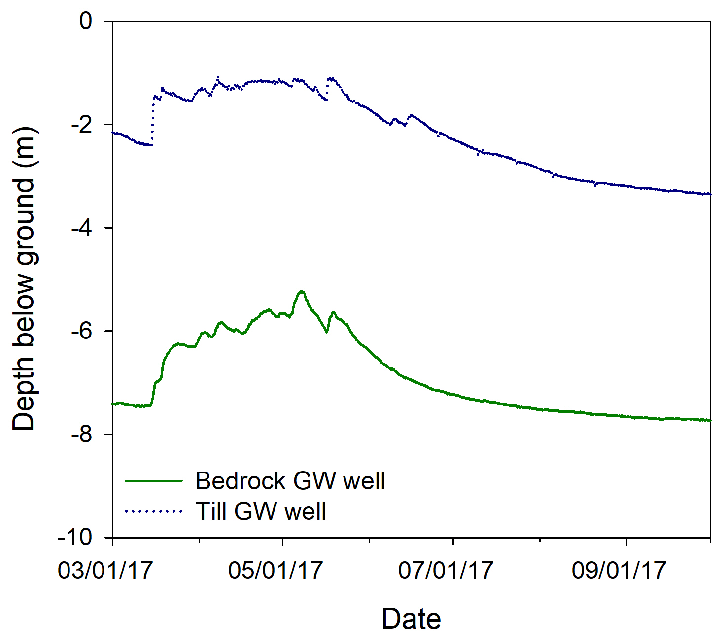
Figure 13Bedrock groundwater and till groundwater well responses (depth below ground in metres) over the 2017 calendar year.
Stream and source water were collected over the 2014 and 2015 water years and visualized using principal components analysis to conceptualize the runoff generation processes in the Canadian Rocky Mountains. While strong variability in source water chemistry limited our ability to quantitatively estimate the relative contributions of multiple water sources to the stream using an unmixing routine, the analyses used here enabled a strong qualitative description of precipitation, hillslope water, and bedrock groundwater source contributions to streamflow. This allowed us to both indirectly observe and infer key runoff generation processes in watersheds with a complex lithological structure characteristic of the highly permeable bedrock and glacial till of the Alberta Rocky Mountain region.
Stream water chemistry in four sub-watersheds of Star Creek showed that Star East (SEL and SEU) and Star West (SWL and SWU) sub-watersheds were more similar than alpine/sub-alpine (SEU and SWU) and upper montane (SEL and SWL) physiographic zones. In general, higher-concentration reacted water reached the stream first at the onset of spring melt in all sub-watersheds. This was followed by a dilution effect as the snowmelt saturated the landscape, and the hillslope was connected to the stream. Fall baseflows differed between Star East and Star West forks. Star West stream water was once again similar to hillslope water or riparian water, but Star East stream water plotted outside the boundary of the measured sources. Seep water temperatures were cool and had low variability, suggesting that it may be deeper bedrock water contributing to the stream. Slower recession rates (and likely lower hydraulic conductivity) in the till groundwater well than in the bedrock groundwater well suggest that water recharged into the till groundwater may be slowly released to the stream. Contamination of the till groundwater well made it unclear when it was contributing to the stream, but groundwater table fluctuations suggested it is likely contributing during late summer or fall. More research on the variability in bedrock and till groundwater chemistry is needed to clarify the difference between these sources and their contributions to streamflow throughout the year. However, it is clear from this research that multiple subsurface flow systems lead to the slow leakage of bedrock and till groundwater to the stream, promoting higher baseflows in this region compared to regions with shallow soils and impermeable bedrock where groundwater stops flowing in the summer.
Please contact the corresponding author regarding data availability.
US and AEA secured the funding that enabled this research and supervised the research project. SAS designed and carried out the field research. SAS analyzed and interpreted the data with assistance from all co-authors and, particularly, ALC with statistics and R code. SAS prepared the original draft of the paper, with contributions from all co-authors in the reviewing and editing thereof.
The authors declare that they have no conflict of interest.
This work would not have been possible without help in the field from Chris Williams, Amanda Martens, Melaina Weiss, Evan Esch, Veronica Martens, Eric Lastiwka, Kirk Hawthorn, Kalli Herlein, Shauna Stack, Chrystyn Skinner, Aryn Sherrit, Erin Cherlet, and Mike Pekrul. We would like to thank Kevin Devito for his contribution to ideas during the initial stages of this research. We would also like to thank the three anonymous reviewers for their comments and suggestions which have substantially improved this paper.
This research has been supported by the National Science and Engineering Research Council (NSERC; grant no. 2006-05497), the Alberta Agriculture and Forestry (grant no. 69GRFD17), Alberta Innovates Water Innovation Program (grant no. 16-009), the Forest Resource Improvement Association of Alberta (grant no. FFI-15-010), and Canadian Forest Products Ltd. Rothamsted Research receives strategic funding from UKRI–BBSRC (UK Research and Innovation Biotechnology and Biological Sciences Research Council). The contribution to this paper by Adrian L. Collins was supported by this grant (grant no. BBS/E/C/000I0330).
This paper was edited by Bettina Schaefli and reviewed by three anonymous referees.
AGS – Alberta Geologic Survey: Bedrock geology of Alberta (GIS data), available at: https://ags.aer.ca/publication/dig-2004-0033 (last access: February 2014), 2004.
Ali, G. A., Roy, A. G., Turmel, A.-C., and Courchesne, F.: Source-to-stream connectivity through end-member mixing analysis, J. Hydrol., 392, 119–135, https://doi.org/10.1016/j.jhydrol.2010.07.049, 2010.
Andres, D., Van Der Vinne, G., and Sterenberg, G.: Hydrologic, hydrogeologic, thermal, sediment and channel regimes of the Tri-Creeks experimental Basin, Rep. No. SWE-87/01, Vol. 1, Alberta Research Council, Edmonton, AB, 418 pp., 1987.
Barthold, F. K., Tyralla, C., Schneider, K., Vaché, K. B., Frede, H. G., and Breuer, L.: How many tracers do we need for end member mixing analysis (EMMA)? a sensitivity analysis, Water Resour. Res., 47, 1–14, https://doi.org/10.1029/2011WR010604, 2011.
Bearup, L. A., Maxwell, R. M., Clow, D. W., and McCray, J. E.: Hydrological effects of forest transpiration loss in bark beetle-impacted watersheds, Nat. Clim. Change, 4, 481–486, https://doi.org/10.1038/nclimate2198, 2014.
Blumstock, M., Tetzlaff, D., Malcolm, I. A., Neutzmann, G., and Soulsby, C.: Baseflow dynamics: Multi-tracer surveys to assess variable groundwater contributions to montane streams under low flows, J. Hydrol., 527, 1021–1033, https://doi.org/10.1016/j.jhydrol.2015.05.019, 2015.
Boon, S.: Snow accumulation following forest disturbance, Ecohydrology, 5, 279–285, https://doi.org/10.1002/eco.212, 2012.
Brown, A. E., Zhang, L., McMahon, T. A., Western, A. W., and Vertessy, R. A.: A review of paired catchment studies for determining changes in water yield resulting from alterations in vegetation, J. Hydrol., 310, 28–61, https://doi.org/10.1016/j.jhydrol.2004.12.010, 2005.
Burles, K. and Boon, S.: Snowmelt energy balance in a burned forest plot, Crowsnest Pass, Alberta, Canada, Hydrol. Process., 25, 3012–3029, https://doi.org/10.1002/hyp.8067, 2011.
Burns, D. A., Murdoch, P. S., Lawrence, G. B., and Michel, R. L.: Effect of groundwater springs on concentrations during summer in Catsill Mountain streams, Water Resour. Res., 34, 1987–1996, 1998.
Christophersen, N. and Hooper, R. P.: Multivariate analysis of stream water chemical data: the use of principal components analysis for the end-member mixing problem, Water Resour. Res., 28, 99–107, https://doi.org/10.1029/91WR02518, 1992.
Clow, D. W., Schrott, L., Webb, R., Campbell, D. H., Torizzo, A., and Dornblaser, M.: Ground water occurrence and contributions to streamflow in an alpine catchment, Colorado front range, Groundwater, 41, 937–950, 2003.
Collins, A. L., Pulley, S., Foster, I. D. L., Gellis, A., Porto, P., and Horowitz, A. J.: Sediment source fingerprinting as an aid to catchment management: A review of the current state of knowledge and a methodological decision-tree for end-users, J. Environ. Manage., 194, 86–108, https://doi.org/10.1016/j.jenvman.2016.09.075, 2017.
Correa, A., Breuer, L., Crespo, P., Célleri, R, Feyen, J., Birkel, C., Silva, C., and Windhorst, D.: Spatially distributed hydro-chemical data with temporally high-resolution is needed to adequately assess the hydrological functioning of headwater catchments, Sci. Total Environ., 651, 1613–1626, https://doi.org/10.1016/j.scitotenv.2018.09.189, 2019.
Covino, T. P. and McGlynn, B. L.: Stream gains and losses across a mountain-to-valley transition: impacts on watershed hydrology and stream water chemistry, Water Resour. Res., 43, W10431, https://doi.org/10.1029/2006WR005544, 2007.
Cowie, R. M., Knowles, J. F., Dailey, K. R., Williams, M. W., Mills, T. J., and Molotch, N. P.: Sources of streamflow along a headwater catchment elevational gradient, J. Hydrol., 549, 163–178, https://doi.org/10.1016/j.jhydrol.2017.03.044, 2017.
Creed, I. F. and Band L. E.: Export of nitrogen from catchments with a temperate forest: evidence for a unifying mechanism regulated by variable source area dynamics, Water Resour. Res., 34, 3105–3120, 1998.
Dahlke, H. E., Easton, Z. M., Lyon, S. W., Walter, M. T., Destouni, G., and Steenhuis, T. S.: Dissecting the variable source area concept – subsurface flow pathways and water mixing processes in a hillslope, J. Hydrol., 420, 125–141, https://doi.org/10.1016/j.jhydrol.2011.11.052, 2012.
Dixon, D., Boon, S., and Silins, U.: Watershed-scale controls on snow accumulation in a small montane watershed, southwestern Alberta, Canada, Hydrol. Process., 28, 1294–1306, https://doi.org/10.1002/hyp.9667, 2014.
Evans, J. E., Prepas, E. E., Devito, K. J., and Kotak B. G.: Phosphorus dynamics in shallow subsurface waters in an uncut and cut subcatchment of a lake on the Boreal Plain, Can. J. Fish. Aquat. Sci., 57, 60–72, 2000.
Floriancic, M. G., van Meerveld, I., Smoorenburg, M., Margreth, M., Naef, F., Kirchner, J. W., and Molnar, P.: Spatio-temporal variability in contributions to low flows in the high Alpine Poschiavino catchment, Hydrol. Process., 32, 3938–3953, https://doi.org/10.1002/hyp.13302, 2018.
Freeze, R. A. and Cherry J. A. (Eds.): Groundwater, Prentice-Hall, New Jersey, USA, 1979.
Freeze, R. A. and Witherspoon P. A.: Theoretical analysis of regional groundwater flow 2. Effect of water-table configuration and subsurface permeability variation., Water Resour. Res., 3, 623–634, 1967.
Goodbrand, A. and Anderson, A.: Hydrologic resilience of a Canadian Foothills watershed to forest harvest, in: EGU General Assembly, 17–22 April 2016, Vienna, Austria, EGU2016-10932, 2016.
Grabs, T., Bishop, K., Laudon, H., Lyon, S. W., and Seibert, J.: Riparian zone hydrology and soil water total organic carbon (TOC): implications for spatial variability and upscaling of lateral riparian TOC exports, Biogeosciences, 9, 3901–3916, https://doi.org/10.5194/bg-9-3901-2012, 2012.
Harder, P., Pomeroy, J. W., and Westbrook, C. J.: Hydrological resilience of a Canadian Rockies headwaters basin subject to changing climate, extreme weather, and forest management, Hydrol. Process., 29, 3905–3924, https://doi.org/10.1002/hyp.10596, 2015.
Hjerdt, K. N., McDonnell, J. J., Seibert, J., and Rodhe, A.: A new topographic index to quantify downslope controls on local drainage, Water Resour. Res., 40, W05602, https://doi.org/10.1029/2004WR003130, 2004.
Hoeg, S., Uhlenbrook, S., and Leibundgut, C.: Hydrograph separation in a mountainous catchment – combining hydrochemical and isotopic tracers, Hydrol. Process., 14, 1199–1216, 2000.
Hood, J. L. and Hayashi, M.: Characterization of snowmelt flux and groundwater storage in an alpine headwater basin, J. Hydrol., 521, 482–497, https://doi.org/10.1016/j.jhydrol.2014.12.041, 2015.
Hooper, R. P.: Diagnostic tools for mixing models of stream water chemistry, Water Resour. Res., 39, 1055, https://doi.org/10.1029/2002WR001528, 2003.
Inamdar, S.: The use of geochemical mixing models to derive runoff sources and hydrologic flow paths, in: Forest hydrology and biogeochemistry: synthesis of past research and future directions, edited by: Levia, D. F., Carlyle-Moses, D., and Tanaka, T., Springer, New York, USA, 163–183, https://doi.org/10.1007/978-94-007-1363-5, 2011.
Inamdar, S., Dhillon, G., Singh, S., Dutta, S., Levia, D., Scott, D., Mitchell, M., Van Stan, J., and McHale, P.: Temporal variation in end-member chemistry and its influence on runoff mixing patterns in a forested, Piedmont catchment, Water Resour. Res., 49, 1828–1844, https://doi.org/10.1002/wrcr.20158, 2013.
James, A. L. and Roulet, N. T.: Investigating the applicability of end-member mixing analysis (EMMA) across scale: a study of eight small, nested catchments in a temperate forested watershed, Water Resour. Res., 42, 1–17, https://doi.org/10.1029/2005WR004419, 2006.
Jencso, K. G., McGlynn, B. L., Gooseff, M. N., Wondzell, S. M., Bencala, K. E., and Marshall, L.A.: Hydrologic connectivity between landscapes and streams: Transferring reach-and plot-scale understanding to the catchment scale, Water Resour. Res., 45, W04428, https://doi.org/10.1029/2008WR007225, 2009.
Jencso, K. G., McGlynn, B. L., Gooseff, M. N., Bencala, K. E., and Wondzell, S. M.: Hillslope hydrologic connectivity controls riparian groundwater turnover: Implications of catchment structure for riparian buffering and stream water sources, Water Resour. Res., 46, W10524, https://doi.org/10.1029/2009WR008818, 2010.
Johannessen, M. and Henriksen, A.: Chemistry of snow meltwater: changes in concentration during melting, Water Resour. Res., 14, 615–619, 1978.
Kienzle, S. W.: A new temperature based method to separate rain and snow, Hydrol. Process., 22, 5067–5085, https://doi.org/10.1002/hyp.7131, 2008.
Langston, G., Bentley, L. R., Hayashi, M., McClymont, A., and Pidlisecky, A.: Internal structure and hydrological functions of an alpine proglacial moraine, Hydrol. Process., 25, 2967–2982, https://doi.org/10.1002/hyp.8144, 2011.
Liu, F., Williams, M. W., and Caine, N.: Source waters and flow paths in an alpine catchment, Colorado Front Range, United States, Water Resour. Res., 40, W09401, https://doi.org/10.1029/2004WR003076, 2004.
McClymont, A. F., Hayashi, M., Bentley, L. R., Muir, D., and Ernst, E.: Groundwater flow and storage within an alpine meadow-talus complex, Hydrol. Earth Syst. Sci., 14, 859–872, https://doi.org/10.5194/hess-14-859-2010, 2010.
McGlynn, B. L. and Seibert, J.: Distributed assessment of contributing area and riparian buffering along stream networks, Water Resour. Res., 39, 1082, https://doi.org/10.1029/2002WR001521, 2003.
McGlynn, B. L., McDonnell, J. J., Shanley, J. B., and Kendall, C.: Riparian zone flowpath dynamics during snowmelt in a small headwater catchment, J. Hydrol., 222, 75–92, https://doi.org/10.1016/S0022-1694(99)00102-X, 1999.
McGlynn, B. L., McDonnell, J. J., and Brammer, D. D.: A review of the evolving perceptual model of hillslope flowpaths at the Maimai catchments, New Zealand, J. Hydrol., 257, 1–26, 2002.
McNamara, J. P., Chandler, D., Seyfried, M., and Achet, S.: Soil moisture states, lateral flow, and streamflow generation in a semi-arid, snowmelt-driven catchment, Hydrol. Process., 19, 4023–4038, https://doi.org/10.1002/hyp.5869, 2005.
Nippgen, F., McGlynn, B. L., and Emanuel, R. E.: The spatial and temporal evolution of contributing areas, Water Resour. Res., 51, 4551–4573, https://doi.org/10.1002/2014WR016719, 2015.
Orlova, J. and Branfireun, B. A.: Surface water and groundwater contributions to streamflow in the James Bay Lowland, Canada, Arct. Antarct. Alp. Res., 46, 236–250, https://doi.org/10.1657/1938-4246-46.1.236, 2014.
Pfister, L., Martínez-Carreras, N., Hissler, C., Klaus, J., Carrer, G. E., Stewart, M. K., and McDonnell, J. J.: Bedrock geology controls on catchment storage, mixing, and release: a comparative analysis of 16 nested catchments, Hydrol. Process., 31, 1828–1845, https://doi.org/10.1002/hyp.11134, 2017.
Pugh E. and Small, E.: The impact of pine beetle infestation on snow accumulation and melt in the headwaters of the Colorado River, Ecohydrology, 5, 467–477, https://doi.org/10.1002/eco.239, 2012.
Pulley, S. and Collins, A. L.: Tracing catchment fine sediment sources using the new SIFT (SedIment Fingerprinting Tool) open source software, Sci. Total Environ., 635, 838–858, https://doi.org/10.1016/j.scitotenv.2018.04.126, 2018.
Pulley, S., Foster, I., and Antunes, P.: The uncertainties associated with sediment fingerprinting suspended and recently deposited fluvial sediment in the Nene river basin, Geomorphology, 228, 303–319, https://doi.org/10.1016/j.geomorph.2014.09.016, 2015.
Rademacher, L. K., Clark, J. F., Clow, D. W., and Hudson, G. B.: Old groundwater influence on stream hydrochemistry and catchment response times in a small Sierra Nevada catchment: Sagehen Creek, California, Water Resour. Res., 41, 1–10, https://doi.org/10.1029/2003WR002805, 2005.
R Core Team: R: A language and environment for statistical computing, R Foundation for Statistical Computing, Vienna, Austria, available at: http://www.R-project.org/ (last access: March 2020), 2014.
Remenda, V. H. and van der Kamp, G.: Contamination from sand-bentonite seal in monitoring wells installed in aquitards, Groundwater, 35, 39–46, 1997.
Rinderer, M., van Meerveld, H. J., and Seibert, J.: Topographic controls on shallow groundwater levels in a steep, prealpine catchment: when are the TWI assumptions valid?, Water Resour. Res., 50, 6067–6080, https://doi.org/10.1002/2013WR015009, 2014.
Scott, D. F.: The hydrological effects of fire in South African mountain catchments, J. Hydrol., 150, 409–432, https://doi.org/10.1016/0022-1694(93)90119-T, 1993.
Shaman, J., Stieglitz, M., and Burns, D.: Are big basins just the sum of small catchments?, Hydrol. Process., 18, 3195–3206, https://doi.org/10.1002/hyp.5739, 2004.
Shanley, J. B., Sebestyen, S. D., McDonnell, J. J., McGlynn, B. L., and Dunne, T.: Water's Way at Sleepers River watershed–revisiting flow generation in a post-glacial landscape, Vermont USA, Hydrol. Process., 29, 3447–3459, https://doi.org/10.1002/hyp.10377, 2015.
Silins, U., Stone, M., Emelko, M. B., and Bladon, K. D.: Sediment production following severe wildfire and post-fire salvage logging in the Rocky Mountain headwaters of the Oldman River Basin, Alberta, Catena, 79, 189–197, https://doi.org/10.1016/j.catena.2009.04.001, 2009.
Silins, U., Anderson, A., Bladon, K. D., Emelko, M. B., Stone, M., Spencer, S. A., Williams, C. H. S., Wagner, M. J., Martens, A. M., and Hawthorn, K.: Southern Rockies Watershed Project, Forest. Chron., 92, 39–42, https://doi.org/10.5558/tfc2016-012, 2016.
Spencer, S. A., Silins, U., and Anderson, A. E.: Precipitation-runoff and storage dynamics in watersheds underlain by till and permeable bedrock in Alberta's Rocky Mountains, Water Resour. Res., 55, 10690–10706, https://doi.org/10.1029/2019WR025313, 2019.
Stednick, J. D.: Monitoring the effects of timber harvest on annual water yield, J. Hydrol., 176, 79–95, https://doi.org/10.1016/0022-1694(95)02780-7, 1996.
Sueker, J. K., Ryan, J. N., Kendall, C., and Jarrett, R. D.: Determination of hydrologic pathways during snowmelt for alpine/subalpine basins, Rocky Mountain National Park, Colorado, Water Resour. Res., 36, 63–75, 2000.
Taniguchi, M.: Evaluation of vertical groundwater fluxes and thermal properties of aquifers based on transient temperature-depth profiles, Water Res., 29, 2021–2026, 1993.
Tromp-van Meerveld, H. J. and McDonnell, J. J.: Threshold relations in subsurface stormflow: 2. The fill and spill hypothesis, Water Resour. Res., 42, W02411, https://doi.org/10.1029/2004WR003800, 2006.
Uchida, T., McDonnell, J. J., and Asano, Y.: Functional intercomparison of hillslopes and small catchments by examining water source, flowpath and mean residence time, J. Hydrol., 327, 627–642, https://doi.org/10.1016/j.jhydrol.2006.02.037, 2006.
Varhola, A., Coops, N. C., Weiler, M., and Moore, R. D.: Forest canopy effects on snow accumulation and ablation: an integrative review of empirical results, J. Hydrol., 392, 219–233, https://doi.org/10.1016/j.jhydrol.2010.08.009, 2010.
Venables, W. N. and Ripley, B. D.: Modern applied statistics with S, 4th Edn., Springer, New York, USA, ISBN 0-387-95457-0, 2002.
Waterline Resources Inc.: Crowsnest River watershed aquifer mapping and groundwater management planning study: TWPS 006 to 009, RGES 01 to 06 W5 Alberta, Report # 2170-12-001, for Oldman Watershed Council, 2013.
Weihs, C., Ligges, U., Luebke, K., and Raabe, N.: klaR analyzing German business cycles, in: Data analysis and decision support, edited by: Baier, D., Decker, R., and Schmidt-Thieme, L., Springer-Verlag, Berlin, Germany, 335–343, 2005.
Williams, C., Silins, U., Bladon, K. D., Martens, A. M., Wagner, M. J., and Anderson, A.: Rainfall-runoff dynamics following wildfire in mountainous headwater catchments, Alberta, Canada, in: American Geophysical Union Fall Meeting, 14–18 December 2015, San Francisco, USA, H34B-06, 2015.
Williams, C. H. S., Silins, U., Spencer, S. A., Wagner, M. J., Stone, M., and Emelko, M. B.: Net precipitation in burned and unburned subalpine forest stands after wildfire in the northern Rocky Mountains, Int. J. Wildland Fire., 28, 750–760, https://doi.org/10.1071/WF18181, 2019.
Williams, M. W., Seibold, C., and Chowanski, K.: Storage and release of solutes from a subalpine seasonal snowpack: soil and stream water response, Niwot Ridge, Colorado, Biogeochemistry, 95, 77–94, https://doi.org/10.1007/s10533-009-9288-x, 2009.
Winkler, R., Spittlehouse, D., and Boon, S.: Streamflow response to clear-cut logging on British Columbia's Okanagan Plateau, Ecohydrology, 10, 1–15, https://doi.org/10.1002/eco.1836, 2017.