The development and persistence of soil moisture stress during drought across southwestern Germany

The drought of 2018 in central and northern Europe showed once more the large impact that this natural hazard can have on the environment and society. Such droughts are often seen as slowly developing phenomena. However, root zone soil moisture deficits can rapidly develop during periods lacking precipitation and meteorological conditions that favor high evapotranspiration rates. These periods of soil moisture stress can persist for as long as the meteorological drought conditions last, thereby negatively affecting vegetation and crop health. In this study, we aim to characterize past soil moisture stress events over the croplands of southwestern Germany and, furthermore, to relate the characteristics of these past events to different soil and climate properties. We first simulated daily soil moisture over the period 1989–2018 on a 1 km resolution grid, using the physically based hydrological model TRAIN. We then derived various soil moisture stress characteristics, including probability, development time, and persistence, from the simulated time series of all agricultural grid cells (n≈15 000). Logistic regression and correlation were then applied to relate the derived characteristics to the plant-available storage capacity of the root zone and to the climatological setting. Finally, sensitivity analyses were carried out to investigate how results changed when using a different parameterization of the root zone, i.e., soil based or fixed, or when assessing soil moisture drought (anomaly) instead of stress. Results reveal that the majority of agricultural grid cells across the study region reached soil moisture stress during prominent drought years. The development time of these soil moisture stress events varied substantially, from as little as 10 d to over 4 months. The persistence of soil moisture stress varied as well and was especially high for the drought of 2018. A strong control on the probability and development time of soil moisture stress was found to be the storage capacity of the root zone, whereas the persistence was not strongly linearly related to any of the considered controls. On the other hand, the sensitivity analyses revealed the increased control of climate on soil moisture stress characteristics when using a fixed instead of a soil-based root zone storage. Thus, the strength of different controls depends on the assumptions made during modeling. Nonetheless, the storage capacity of the root zone, whether it is a characteristic of the soil or a difference between a shallow or deep rooting crop, remains an important control on soil moisture stress characteristics. This is different for SM drought characteristics, which have little or contrasting relation with the storage capacity of the root zone. Overall, the results give insight to the large spatial and temporal variability in soil moisture stress characteristics and suggest the importance of considering differences in root zone soil storage for agricultural drought assessments.

1 Introduction

Droughts are naturally (re-)occurring phenomena that can appear in different domains of the hydrological cycle and cause associated impacts (Tallaksen and Van Lanen, 2004; Stahl et al., 2016). Because of their multifaceted characteristics, droughts are often classified as different types (Wilhite and Glantz, 1985). Of these drought types, one is agricultural drought, which refers to the impact of lacking water availability on the health and growth of crops. These agricultural droughts can reduce yields and, thereby, cause large economic losses. A crucial first step for reducing the risk of (agricultural) drought impacts involves the effective monitoring and early warning of the drought hazard (UN/ISDR, 2009). Agricultural drought monitoring and early warning occurs at different scales, from plot-scale observations and simulations to regional-scale drought mapping. Regional-scale drought monitoring and early warning provides an overview of regions at drought risk, which raises awareness and helps decision-making. Accurately depicting areas affected by agricultural drought is complex, as its occurrence is influenced by a variety of factors, often including spatially heterogeneous climate and soil characteristics. A better understanding of how these climate and soil characteristics control (the development of) agricultural droughts is needed.

Droughts are often defined as a below-normal water availability, with the normal often depending on space and time (Tallaksen and Van Lanen, 2004). Such an anomaly-based definition allows the depiction of regions and episodes with below-normal water availability across the world, according to different hydro-meteorological variables. However, the identified events with below-normal water availability might not necessarily have the potential to cause drought-related impacts. The below-normal definition of drought forms the basis of many drought indices, which reflect whether a certain hydro-meteorological variable is anomalously low or high (e.g., Anderson et al., 2007; McKee et al., 1993; Samaniego et al., 2012; Vicente-Serrano et al., 2010). Soil moisture anomaly time series, or proxies of the latter, are often used for agricultural drought assessments (e.g., Sheffield et al., 2004; Andreadis et al., 2005; Samaniego et al., 2012). Different drought characteristics can be derived from these soil moisture anomaly time series, including drought magnitude, duration, and areal extent.

The data used for agricultural drought assessments stem from different sources. These data sources include direct soil moisture measurements, remote sensing observations, meteorological proxies, and hydrological or land surface model simulations (e.g., Berg and Sheffield, 2018). Soil moisture measurements provide the most realistic information about the soil moisture status at a certain depth but are point based and, thereby, limited in their spatial coverage. Remote sensing observations of soil moisture provide regional coverage but direct observations are only able to detect soil moisture changes in the upper soil layer, at least in the case of microwave remote sensing. On the other hand, remote sensing observations of heat fluxes and vegetation health can provide an estimate of the ratio between actual and potential evapotranspiration and, thereby, depict regions with soil moisture stress (e.g., Anderson et al., 2007). Meteorological proxies for agricultural drought include drought indices such as the Palmer Drought Severity Index (PDSI; Palmer, 1965) or standardized precipitation evapotranspiration index (SPEI; Vicente-Serrano et al., 2010). The strength of these meteorological proxies is their relative ease of computation and often low data requirements. However, meteorological proxies are often based on potential evapotranspiration and do not consider some other relevant terrestrial processes that influence soil moisture and agricultural drought, such as the reduction in evapotranspiration during soil moisture stress. Many of these terrestrial processes are included in physically based hydrological and land surface models. The physical basis of these models makes their use often preferable over the use of meteorological proxies for past and future agricultural drought assessments (e.g., Berg and Sheffield, 2018; Sheffield et al., 2012).

Various hydrological and land surface models have been used to assess past and future soil moisture drought events. An example is the Variable Infiltration Capacity (VIC) model, which has been applied to characterize major soil moisture drought episodes across different regions (e.g., US – Sheffield et al., 2004, and Andreadis et al., 2005; China: Wang et al., 2011; and globally – Sheffield and Wood, 2007). The latter analyses enabled the cataloguing of past soil moisture drought events according to a variety of characteristics, providing a benchmark for current and future drought events. Another example of a regionally applied model for the simulation of soil moisture (drought) is the mesoscale Hydrological Model (mHM; Samaniego et al., 2010). The output of the mHM has been used for both historic soil moisture drought assessments (Hanel et al., 2018) and for future soil moisture drought projections according to different climate change scenarios across Europe (as part of a model ensemble in Samaniego et al., 2018). The latter studies provide valuable insights about the severity of recent soil moisture drought events over Europe, e.g., 2003 and 2015, and also show that these recent events were not as rare when considered from a more long-term historical perspective, and that similar or worse events are more likely to occur under different climate change scenarios. The mHM is also run in near-real time, and its output is used by the German Drought Monitor (Zink et al., 2016).

Studies mentioned in the previous paragraph focus on characterizing past and future soil moisture drought events, whereas other studies aim to characterize its development. Drought is often referred to as a slowly developing phenomena that can take up to years to reach its full extent (Wilhite and Glantz, 1985). However, not all drought events are slowly developing phenomena, and soil moisture deficits can develop relatively quickly during dry weather conditions that favor high amounts of evapotranspiration (e.g., Hunt et al., 2009). These rapidly developing droughts, sometimes termed flash droughts, can severely impact agriculture (e.g., Svoboda et al., 2002; Otkin et al., 2018). Several case study flash drought events in the US have been described in Otkin et al. (2013, 2016). The latter studies show that precipitation deficits can be quickly followed by a reduction in evapotranspiration, which is indicative of low soil moisture levels, causing water stress for plants. Christian et al. (2019) aimed to make a regional assessment of past flash droughts and developed a framework of objective criteria to identify flash drought events from simulated soil moisture output. By applying this framework to soil moisture simulations over the US, they show that particular regions, such as the Great Plains, are more sensitive to flash drought occurrence.

Most of the above-described soil moisture drought assessments characterize drought as a below-normal anomaly according to different hydrometeorlogical variables, which is in line with the traditional definition of drought. However, from an agricultural drought impact perspective, it can make more sense to directly study the characteristics of (the development of) periods of lacking amounts of root zone soil moisture, i.e., soil moisture stress, which is in line with the soil moisture drought index proposed in Hunt et al. (2009). Following this reasoning, and being inspired by the methods used in previous soil moisture anomaly studies, we aim to study simulated soil moisture stress events across the agricultural regions of southwestern Germany. Our objectives are as follows:

1. characterize past soil moisture stress events,

2. investigate dominant controls on soil moisture stress characteristics, and

3. portray meteorological anomalies during (the development of) soil moisture stress.

Finally, we aim to carry out a sensitivity analyses to investigate how derived (controls on) characteristics change when using different parameterizations of the root zone soil or when investigating soil moisture drought instead of soil moisture stress.

2 Data and methods

2.1 Study region

The study region encompasses Baden-Württemberg (area ≈ 36 000 km²), a federal state of Germany located in the southwestern part of the country (Fig. 1). The area of interest covers both flat and lowland regions, such as the Rhine valley, and higher, more mountainous regions, such as the Black Forest and the Swabian Jura (Fig. 1a). The topography of the study region affects both temperature (annual average (T_annual) between 4.5 and 11.6 ^∘C; Fig. 1b) and precipitation (annual average sum (P_annual) between < 600 and > 2000 mm; Fig. 1c). Land cover and soil characteristics vary over the study region (Fig. 1d, e). Most of the cropland, on which this study focuses, is located in the lower areas (Fig. 1d). Thicker soils with a higher available water-holding capacity (AWC in millimeters; i.e., the amount of plant-available water in the root zone at field capacity) are generally found in the valleys and more shallow soils with a lower AWC in the elevated, mostly forested regions (Fig. 1d, e).

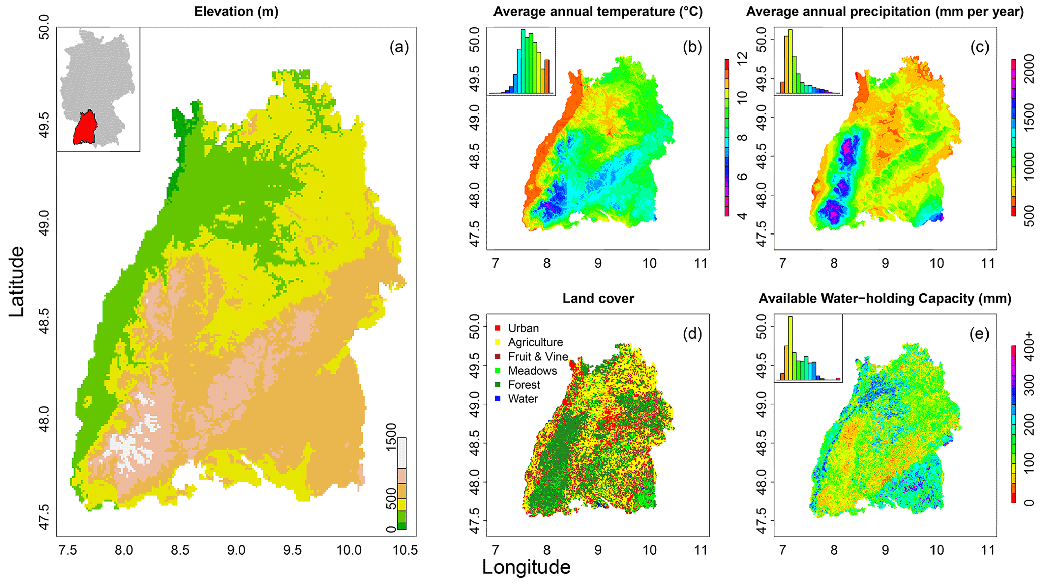
Figure 1 Study region and its (a) elevation, (b) average annual temperature, (c) average annual precipitation sum, (d) land cover, and (e) available water-holding capacity of the root zone soil. Gridded data used to derive this figure are described in Sect. 2.2.

2.2 Data and interpolation

The data used in this study stem from various sources. Gridded elevation data (1 km resolution) were obtained from the Federal Agency for Cartography and Geodesy (BKG, 2019). Vectorized land cover data come from the Corine 2006 data set and were retrieved from the German Environment Agency (UBA, 2019). Vectorized soil property data (field capacity, wilting point, air capacity, and depth of the root zone soil based on soil properties of different layers) were derived from the BK-50 (scale of 1:50 000) data set provided by the Federal State Office for Geology Resources and Mining (LGRB, 2019). River flow data come from the Environment Agency of Baden-Württemberg (LUBW). Daily meteorological data for the period between 1989 and 2018 used in this study stem from both gridded data and station-based observations. Gridded precipitation (P millimeters) comes from the REGNIE (Regionalisierte Niederschlagshöhen) data set (Rauthe et al., 2013) and was sourced from the climate data center of the German Weather Service (DWD, 2019). Gridded satellite-based global radiation data (W m⁻²) stem from the SARAH data set and were derived from the Satellite Application Facility on Climate Monitoring (CM SAF; Pfeifroth et al., 2019a, b). Station-based meteorological observations of temperature (T; degrees Celsius), relative humidity (percent), and sunshine duration (hours) as well as subdaily observations of wind speed (Bft) and wind direction (degrees) originate from the climate data center of the German Weather Service (DWD, 2019). The subdaily values of wind speed and wind direction were aggregated to daily values (for wind speed – arithmetic average; for wind direction – average of Cartesian coordinates).

All data were interpolated to 1 km resolution grids covering Baden-Württemberg. Land cover and soil property data were interpolated based on the majority class within each grid cell. Gridded meteorological data were reprojected to match the extent and resolution of the soil and land cover grids. Station-based meteorological observations were interpolated to grids using the INTERMET software (Dobler et al., 2004; software ran in default settings). The software first converts (the units of) some of the meteorological observations, i.e., wind speed (Bft) to wind speed (meters per second) and sunshine duration to global radiation. The software then interpolates these (and all other) meteorological observations to daily grids, using different kriging-based interpolation techniques. These interpolation techniques consider distance to the station and, depending on the variable, the possible relationship between the variable of interest and other external factors, such as elevation, wind direction, or relief. The grids of global radiation interpolated with INTERMET were only used for days for which the SARAH data set did not provide any data (< 0.25 % of days).

2.3 Soil moisture modeling

We applied the physically based hydrological model TRAIN (TRAnspiration and INterception; indicating the major processes considered during the initial phase of model development; Fig. 2). The model was used to simulate different fluxes, such as the different components of evapotranspiration (E_total) and percolation (Q_percolation), and stores, such as soil moisture (SM), at a daily resolution over Baden-Württemberg. The TRAIN model follows some basic principles, of which the most important are the applicability of the model on both the plot and the areal scale (e.g., Stork and Menzel, 2016; Törnros and Menzel, 2014) and the ability to run the model with as few input data as possible, which benefits its general applicability on larger scales. TRAIN includes information from comprehensive field studies of the water and energy balance for different surface types, including natural vegetation and cropland (Menzel, 1997; Stork and Menzel, 2016). Special focus in the model is on the water and energy fluxes at the soil–vegetation–atmosphere interface.

Figure 2 Conceptual flow chart of the fluxes and stores considered in TRAIN.

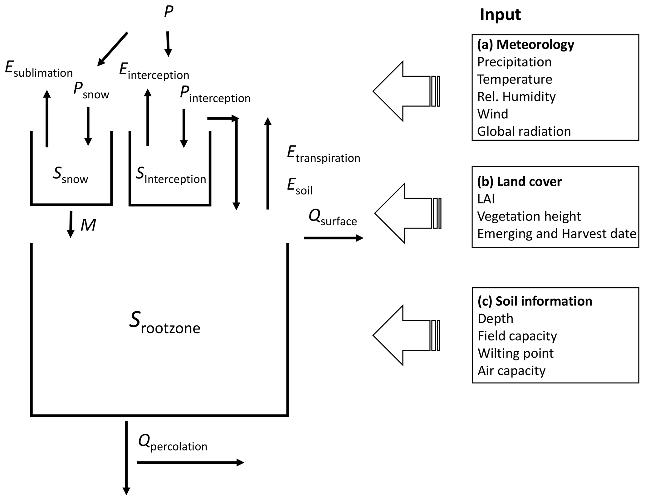
In brief, the model works as follows. First, precipitation is divided into either rain (P_rain) or snow (P_snow), depending on whether the daily average T exceeds the threshold temperature (T_threshold= 0 ^∘C) or not. P_snow is temporarily accumulated in a snow storage reservoir (S_snow), which grows via the accumulation of P_snow or shrinks via melt (M; occurring when T > T_threshold and derived using the degree day method; Kustas et al., 1994) or sublimation (E_sublimation; derived following the Penman–Monteith equation, with canopy resistances set to zero; Wimmer et al., 2009). P_rain is either stored as interception (S_interception), where the size of S_interception depends on the leaf area index (LAI) or bypasses the interception reservoir if it is (partly) filled or nonexistent. Water is removed from the interception reservoir via evaporation (E_interception), which is modeled to occur at different intensities as a function of the S_interceptionand the present meteorological conditions (Menzel, 1997). P_rain and M either infiltrate in the root zone storage reservoir (S_rootzone) or generate surface runoff (Q_surface). The total water storage capacity of S_rootzone is divided into different parts, i.e., immobile water (the volume of water below wilting point) plant-available water (the volume of water between permanent wilting point and field capacity; also referred to as AWC), and excess water (volume of water above field capacity; constrained by the total porosity of the root zone soil). Q_surface is only generated when S_rootzone is saturated and P exceeds an intensity threshold of 20 mm per day. The simulation of transpiration (E_{transpiration}) is based on the Penman–Monteith equation. It depends on the calculation of canopy resistances, which are modified by the state of growth of the vegetation, the status of S_rootzone, and the meteorological conditions (Menzel, 1996; Fig. 2a). The calculation of percolation (Q_percolation) follows the conceptual approach from the HBV model (Bergström, 1995) and occurs at a rate that is a function of the amount of excess water in the root zone.

Vegetation development, i.e., the temporal dynamics of LAI and vegetation height and emerging and harvest date, in the case of agriculture, are related to land cover properties (Fig. 2b). These land cover properties were derived from the Corine data set (Sect. 2.2), which encompasses general land use classes, such as broadleaved forest or agriculture. Each of these land use classes were assigned associated temporally varying vegetation properties that are typical for the study region. For the agricultural grid cells on which we focus in this study, we considered a mixed parameterization of typical agricultural crops of the region. It should be noted that, in reality, there are crop-specific differences that further vary in space and time due to, for example, spatiotemporal differences in climate or temporal changes in climate or genotypes (e.g., Bohm et al., 2020; Ingwersen et al., 2018; Rezaei et al., 2018). However, given the absence of detailed spatiotemporal information over the region about these differences, we used the generalization as described above.

S_rootzone was derived from soil properties from the BK-50 data set (Sect. 2.2; Fig. 2c). This data set is based on extensive field investigations on soil profiles distributed over the whole of Germany, which led to a detailed soil map, including information about soil types, grain size distribution, sequence, and depth of soil horizons as well as parameters describing the water-holding capacity (field capacity, wilting point, and air potential). In addition, it includes information about the potential depth of the root zone, broadly ranging between a few decimeters up to 2 m and constraint by, for example, the occurrence of a root restrictive layer. In addition to soil properties, other factors, such as plant type, climate, and meteorological conditions during certain growth stages, influence how deep plant roots grow and, thereby, the AWC of the root zone (e.g., Fan et al., 2016; de Boer-Euser et al., 2016). However, we used the above-described soil-based parameterization of S_rootzone (more commonly used in regional modeling studies), as detailed spatiotemporal information about these other factors are unknown, and the used soil-based parameterization provides a reasonable boundary condition.

The initial conditions of S_rootzone were set to field capacity at the start of the model run on 1 January 1988. The first year (1988) was used as the warm-up year, whereas the following 30 years (1989–2018) were used for the analyses. A longer warm-up was not needed for the purpose of this study, given that only the amount of snow that accumulated in the winter of 1988–1989 affected the considered fluxes and stores over the studied period. Snapshots of the soil moisture status during different stages of the drought year 2018 are shown in Fig. 3; complete daily animations of soil moisture status during different drought years are provided in the associated online repository (Tijdeman and Menzel, 2021).

Figure 3 Simulated soil moisture (expressed as the percent of available water-holding capacity, AWC, left in the root zone) during different stages of the drought of 2018.

In this study, we specifically analyzed simulated soil moisture (SM; expressed as the percent of AWC left in the root zone) and total evapotranspiration (E_total, mm d⁻¹). For the SM stress analyses, we focus on grid cells classified as agricultural, as the focus of this study is on agricultural drought. Simulations of grid cells of other land uses were only considered for the model evaluation.

2.4 Model evaluation

On the plot scale, the performance of TRAIN was evaluated against observed SM and E in various previous studies (e.g., Sect. 2.3). However, such observations are scarcely available on the regional scale. Therefore, evaluation of the simulated fluxes and states vs. observed streamflow is helpful for obtaining insight with respect to whether these are reasonable or not. Given that TRAIN is not a rainfall–runoff model, a direct comparison between daily streamflow simulations and observations (Q_observed) is not possible (Fig. 2). Instead, we evaluated, for 60 catchments with near-natural flow located across the study region (Fig. S1 in the Supplement), whether the following conditions are met:

1. The average annual water balance is comparable ($Q_{\mathrm{percolation}}+Q_{\mathrm{runoff}}+\mathrm{\Delta }S\approx Q_{\mathrm{observed}}$), where ΔS is the change in catchment storage over the period of record.

2. The annual water balance is comparable and correlated.

3. The monthly sums of Q_observed are correlated with the sum of Q_percolation and Q_runoff accumulated over a catchment-specific time window of n months.

4. The gradual drying of simulated SM during meteorological drought is also visible for part of the Q_observed time series, i.e., those without a large groundwater flow contribution that can sustain low flows.

5. The event or quick flow mainly occurs when simulated SM exceeds field capacity for most grid cells within the catchment.

Several storage components encompassed in ΔS, e.g., S_snow or S_rootzone, are simulated in the TRAIN model; however, groundwater is not (Fig. 2). For the first criterion, the impact of not considering groundwater in ΔS is relatively small as the sums of P, E_total, and Q_observed over the considered period are much larger. For the second and fourth criteria, not considering groundwater in ΔS can have a larger influence, especially for catchments with extensive groundwater stores that can buffer low flows even though S_rootzone is depleted. For the third criterion, we considered differences in catchment response using the following approach (inspired from Barker et al., 2016). We first accumulated the sum of Q_percolation and Q_runoff over n-month periods (1–12 months), i.e., for each month the sum of Q_percolation and Q_runoff in the current month, the current and previous month, etc. (similar to the calculation of the SPEI-n). Thereafter, we correlated monthly Q_observed with the sum of Q_percolation and Q_runoff accumulated over the different n-month periods for each catchment and calendar month. In the end, we selected, for each catchment and calendar month, the accumulation period with the maximum correlation with Q_observed.

2.5 Soil moisture stress characteristics

We identified SM stress events, i.e., events where SM was continuously at or below a threshold (τ) from all daily simulated SM time series of agricultural grid cells. In this study, τ was set to 30 % of the AWC (i.e., 30 % of available water left in the root zone), which is in line with the threshold used by the German Weather Service to define possible low-water stress (DWD, 2018). Various characteristics were calculated for the identified SM stress events. We first created a binary time series of annual SM stress occurrence (S_occ) for each agricultural grid cell (i= 1, 2 … 15 359) and calendar year (y= 1989, 1990 … 2018), which indicates, for each grid cell and each year, whether SM stress was reached ($S_{\mathrm{occ},i,y}=$ 1) or not ($S_{\mathrm{occ},i,y}=$ 0). Then, if $S_{\mathrm{occ},i,y}=$ 1, i.e., grid cell i reached SM stress in year y, various other SM stress characteristics were derived for that grid cell and year, as follows:

• $S_{\mathrm{start},i,y}$ – the first day of SM stress (doy – day of year);

• $S_{\mathrm{devtime},i,y}$ – the development time of SM stress (in days), i.e., the time it took to drop from field capacity (last day) to SM stress (first day);

• $S_{\mathrm{total},i,y}$ – the total time in SM stress (in days), i.e., the number of days SM_i,y < τ; and

• $S_{\mathrm{maxdur},i,y}$ – the maximum duration of SM stress (in days), i.e., the maximum number of consecutive days with SM_i,y<τ.

These different SM stress characteristics are exemplified in Fig. 4. In this study, SM stress episodes were defined based on the percentage of water left in the soil. Thus, SM stress differs from SM drought, which is expressed as an anomaly.

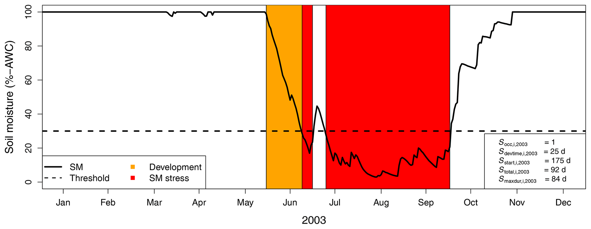
Figure 4 Simulated soil moisture (SM) time series of an exemplary agricultural grid cell, showing the development and persistence of SM stress in 2003. The considered SM stress characteristics are presented in the lower-right legend, i.e., whether SM stress developed or not ($S_{\mathrm{occ},i,\mathrm{2003}}$), the development time ($S_{\mathrm{devtime},i,\mathrm{2003}}$), first day ($S_{\mathrm{start},i,\mathrm{2003}}$), total number of days ($S_{\mathrm{total},i,\mathrm{2003}}$), and maximum duration ($S_{\mathrm{maxdur},i,\mathrm{2003}}$). In this plot, the SM time series is capped at 100 % AWC.

2.6 Controls on simulated SM stress characteristics

We related the derived SM stress characteristics in different years (y) to the soil properties (AWC; Fig. 1e) and climatological setting (T_annual and P_annual; Fig. 1b, c). A total of two different techniques were used, as follows:

1. Logistic regression for the binary data of S_occ,y;

2. Spearman's rank correlation for the integer time series of S_start,y, S_devtime,y, S_total,y and S_maxdur,y.

Both the logistic regression and correlation analyses were carried out for each year, separately, to investigate whether the results were consistent over the years or exhibited a year-to-year variability.

2.7 Meteorological anomalies during (the development of) SM stress

We further characterized the meteorological anomalies during (the development of) SM stress. For all grid cells and years (and when S_occ= 1), we calculated anomalies of P, T, and E_total (percentiles; respectively $P_{\mathrm{perc},i,y}$, $T_{\mathrm{perc},i,y}$, and $E_{\mathrm{perc},i,y}$) during both the development (dev) and annual maximum duration (maxdur) of SM stress. Weibull plotting positions were used to calculate these percentiles, i.e., rank(x)$/$(n+1), where x is the meteorological variable of interest, and n is the sample size (in this study, n equals 30 years). The time window for which these percentiles were derived matches the time window of development and annual maximum duration. For the example in Fig. 4, SM stress developed between 31 May and 24 June and had its maximum duration between 10 July and 1 October 2003. For this event, $P_{\mathrm{perc},\mathrm{dev},i,\mathrm{2003}}$, $T_{\mathrm{perc},\mathrm{dev},i,\mathrm{2003}}$, and $E_{\mathrm{perc},\mathrm{dev},i,\mathrm{2003}}$ ($P_{\mathrm{perc},\mathrm{maxdur},i,\mathrm{2003}}$, $T_{\mathrm{perc},\mathrm{maxdur},i,\mathrm{2003}}$, and $E_{\mathrm{perc},\mathrm{maxdur},i,\mathrm{2003}}$) express the meteorological anomalies of the period between 31 May and 24 June (10 July and 1 October) in 2003, relative to the same time window in all other years.

For ease of notation, we omit the grid cell identifiers (i) and, where applicable, year identifiers (y) from the variable subscripts in the remainder of this paper.

2.8 Sensitivity to the parameterization of S_rootzone and used identification method

The AWC of S_rootzone was derived from properties of the root zone soil (Sect. 2.3; from now on referred to as soil-based S_rootzone). To investigate the sensitivity of the derived (controls on) simulated SM stress characteristics to the parameterization of the S_rootzone, we carried out the same analyses but with simulations derived using different root zone parameterizations. For one parameterization, the AWC of the root zone was again based on soil properties, but the depth of the root zone soil was constraint at 1 m, placing a fixed lower boundary on rooting depth. For two other parameterizations, we fixed the size of the AWC of S_rootzone to 100 and 200 mm, respectively, aiming to differentiate between (more shallow rooting) crops with a lower water availability and (deeper rooting) crops with a higher water availability.

SM stress episodes were defined based on the percentage of plant-available water left in the root zone soil. However, given that percentage of water left in the soil differs from SM anomalies commonly used for drought studies, we carry out a sensitivity analyses to investigate how (controls on) SM stress characteristics differ from (controls on) SM anomaly characteristics, hereafter referred to as SM drought. For this comparison, daily SM values were first transferred to anomaly space using Weibull plotting positions (Sect. 2.7), thus ranking daily SM values of a certain calendar day and year compared to SM values of the same calendar day in other years. The 20th percentile threshold commonly used for drought studies was used to extract drought episodes from the SM anomaly time series. Then, (controls on) the characteristics of these drought episodes were derived in the same way as was done for SM stress episodes (Sect. 2.5–2.6).

3 Results

3.1 Model evaluation

Overall, annual average Q_observed reveals a good agreement with the sum of annual average simulated Q_percolation and Q_runoff (Fig. 5a). Differences are mostly within the 100 mm range, with few exceptional catchments showing slightly larger differences, especially in the wetter domains of the study region encompassing mostly forested catchments. Systematic biases related to the catchment average AWC of the root zone were not observed. Figure 5b reveals the distribution of Spearman's rank correlation coefficients between annual Q_observed and the simulated annual sum of Q_percolation and Q_runoff (averages over the hydrological year) for all catchments. The generally high correlation coefficients indicate that TRAIN simulates the interannual variability more or less correctly, especially when considering that TRAIN does not have a baseflow reservoir and, therefore, is not able to simulate (annual) variability in groundwater storage. On the monthly scale, the correlation between Q_observed and the sum of Q_percolation and Q_runoff accumulated over the n-month period, with the highest correlation with Q_observed, indicated a good agreement (Fig. S2). Furthermore, their percentile time series were comparable during prominent drought years 2003 and 2018 (Fig. S3a–d). In addition, episodes with anomalously low SM generally coincide with episodes of anomalously low river flow, as is exemplified for drought years 2003 and 2018 in Fig. S3. Finally, Figs. S4 and S5 reveal that a relatively large proportion of precipitation contributes to event flow whenever S_rootzone of all grid cells within the catchment are filled to a level at or above field capacity. This relative contribution of precipitation to event flow strongly declines whenever a large proportion of grid cells within the catchment drops to a level below field capacity.

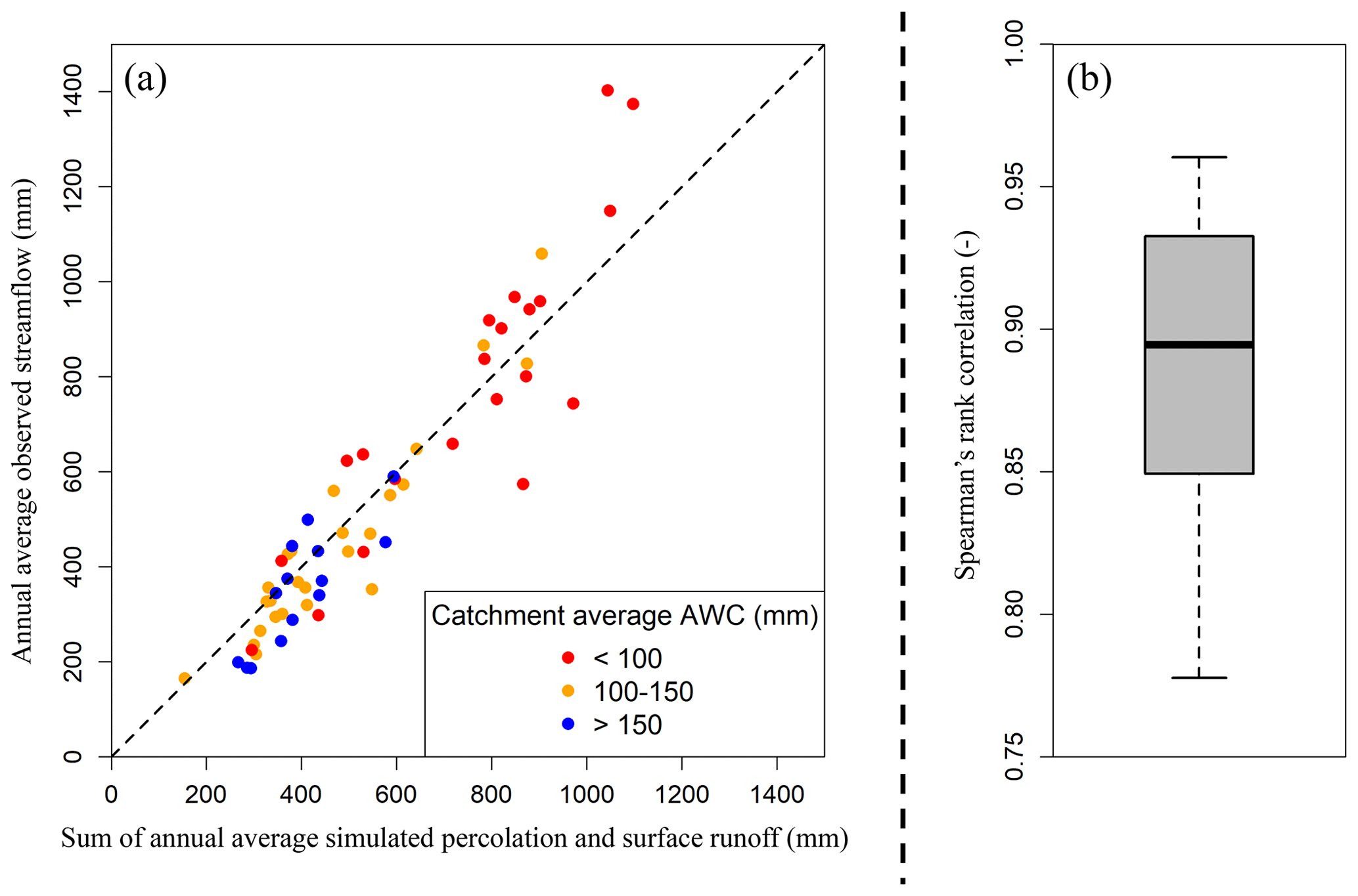
Figure 5 (a) Annual average Q_observed vs. the annual average sum of simulated Q_percolation and Q_runoff (each dot reflects one catchment; colors of the dots indicate catchment average AWC; dashed red line is the 1:1 line), and (b) the distribution of Spearman's rank correlation between annual Q_observed and the sum of simulated annual Q_percolation and Q_runoff, considering hydrological years (October–September) for all considered catchments. The box shows the 25th, 50th, and 75th percentile, and the end of the whiskers shows the 5th and 95th percentile.

3.2 (Controls on) past SM stress characteristics

Figure 6 presents the percentage of grid cells that reached SM stress at least once in different calendar years (S_occ= 1). In general, results reveal a large temporal variability in the fraction of cells that reached SM stress. SM stress was reached in all years for at least a small proportion of the cells. However, the most prominent drought years (i.e., the years in which most cells reached SM stress) were 2003 and 2018, followed by 2015 and 1991. During these years, up to 89 % of the grid cells reached SM stress.

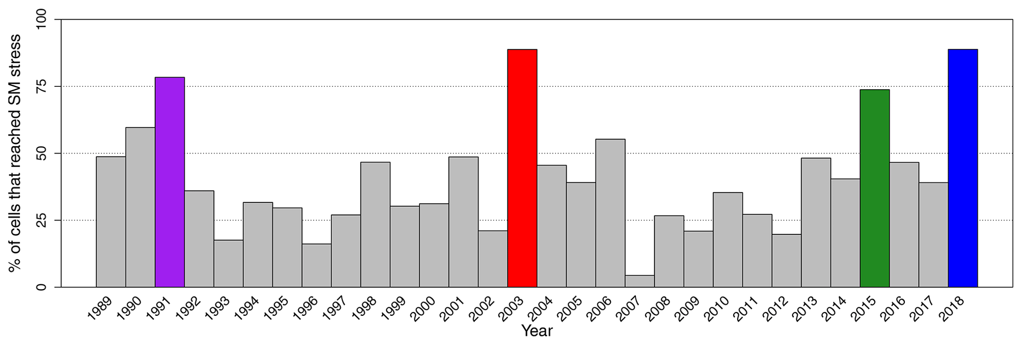
Figure 6 Percentage of cells that reached soil moisture stress for at least 1 d (S_occ= 1) in different calendar years. The most prominent years (1991, 2003, 2015, and 2018) are highlighted in color.

Figure 7 shows the relationship between the probability of reaching SM stress (S_occ) and different controls (AWC; P_annual; T_annual). In general, probability functions derived with the AWC show a steeper and annually consistent increase than probability functions derived with P_annual and T_annual. The latter suggests a stronger influence of root zone soil characteristics, compared to the influence of the climatological setting, on whether or not SM stress developed. SM stress was, furthermore, found to be more likely to develop in soils that have a lower AWC (Fig. 7a), as the probability of S_occ increases with decreasing AWC. The direction of increasing probability was consistent for every year, i.e., grid cells with a lower AWC always had a higher probability of reaching SM stress than grid cells with a higher AWC. However, during the most prominent drought years, the probability functions are shifted to the right, revealing a higher probability of reaching SM stress for grid cells with a higher AWC during these dry years. SM stress was further found to be more likely to develop in drier regions with a lower P_annual (Fig. 7b). The probability of SM stress as a function of T_annual shows more variation in the direction of increasing probability (Fig. 7c). In some years, including the prominent drought years, SM stress was more likely to develop in the warmer regions, whereas in some other years, no strong relationship with temperature was observed.

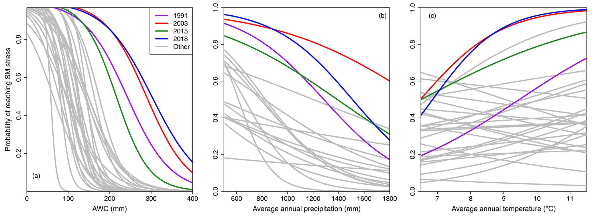
Figure 7 Probability of reaching SM stress at least once in a year (S_occ= 1) as a function of (a)  the AWC, (b)  P_annual, and (c) T_annual. Each curve reflects a different year, and the curves of prominent drought years are highlighted in color.

Figure 8 shows the variation in SM stress characteristics. In general, there was a lot of within-year variability in these characteristics, whereas differences between prominent drought years were often less pronounced. S_start varies from the end of April to the end of September (Fig. 8a). The distributions of S_start are comparable between 2003, 2015, and 2018, whereas the distribution of S_start of 1991 indicates a generally later onset of SM stress. S_devtime shows a large variability, from as little as 10 d to over 4 months (Fig. 8b). Despite the large within-year variability of S_devtime, there were no evident differences in the development time distributions among the prominent years. S_total shows both a large within-year variability and distinct differences among the prominent drought years (Fig. 8c). The distributions of S_total reveal that 2003 and especially 2018 were characterized by the longest total time in SM stress (median $S_{\mathrm{total},\mathrm{2018}}=$ 91 d; 95th quantile $S_{\mathrm{total},\mathrm{2018}}=$ 151 d). Similar within-year variability and between-year differences were found for S_maxdur (Fig. 8d). Especially 2018 was characterized by persistent SM stress events (median S_maxdur,2018 of 79 d; 95th percentile of 147 d).

Table 1 reveals Spearman's rank correlation coefficient between various SM stress characteristics and the AWC of the root zone and the climatological setting (P_annual, T_annual) during prominent drought years. Both S_start and S_devtime were most strongly correlated with the AWC, whereas the correlation with P_annual or T_annual was weaker or absent. These correlations imply that the start of soil moisture stress tends to be later, and the development time tends to be longer, for soils with a higher AWC. The correlations between the persistence of SM stress (S_total and S_maxdur) and the considered soil and climate controls suggest that the time in soil moisture stress tends to be longer for soils with a lower AWC that are located in drier and warmer domains of the study region. However, the correlations were often weak or nonexistent, and the sign of the correlation coefficient was not always consistent.

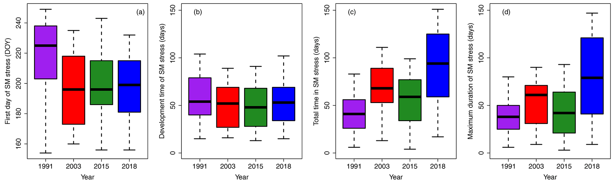
Figure 8 Variability in different SM stress characteristics shown for the prominent drought years. Shown are the (a) first day (S_start), (b) development time (S_devtime) (c) total number of days (S_total), and (d) maximum duration (S_maxdur) of SM stress. The box shows the 25th, 50th, and 75th percentile, and the end of the whiskers shows the 5th and 95th percentile.

Table 1 Spearman's rank correlation coefficient between SM stress characteristics and soil and climate controls for 4 prominent drought years. Considered SM stress characteristics are first day (S_start), development time (S_devtime), total time (S_total), and maximum duration (S_maxdur). Considered controls are available water-holding capacity of the root zone (AWC), annual average precipitation (P_annual), and annual average temperature (T_annual).

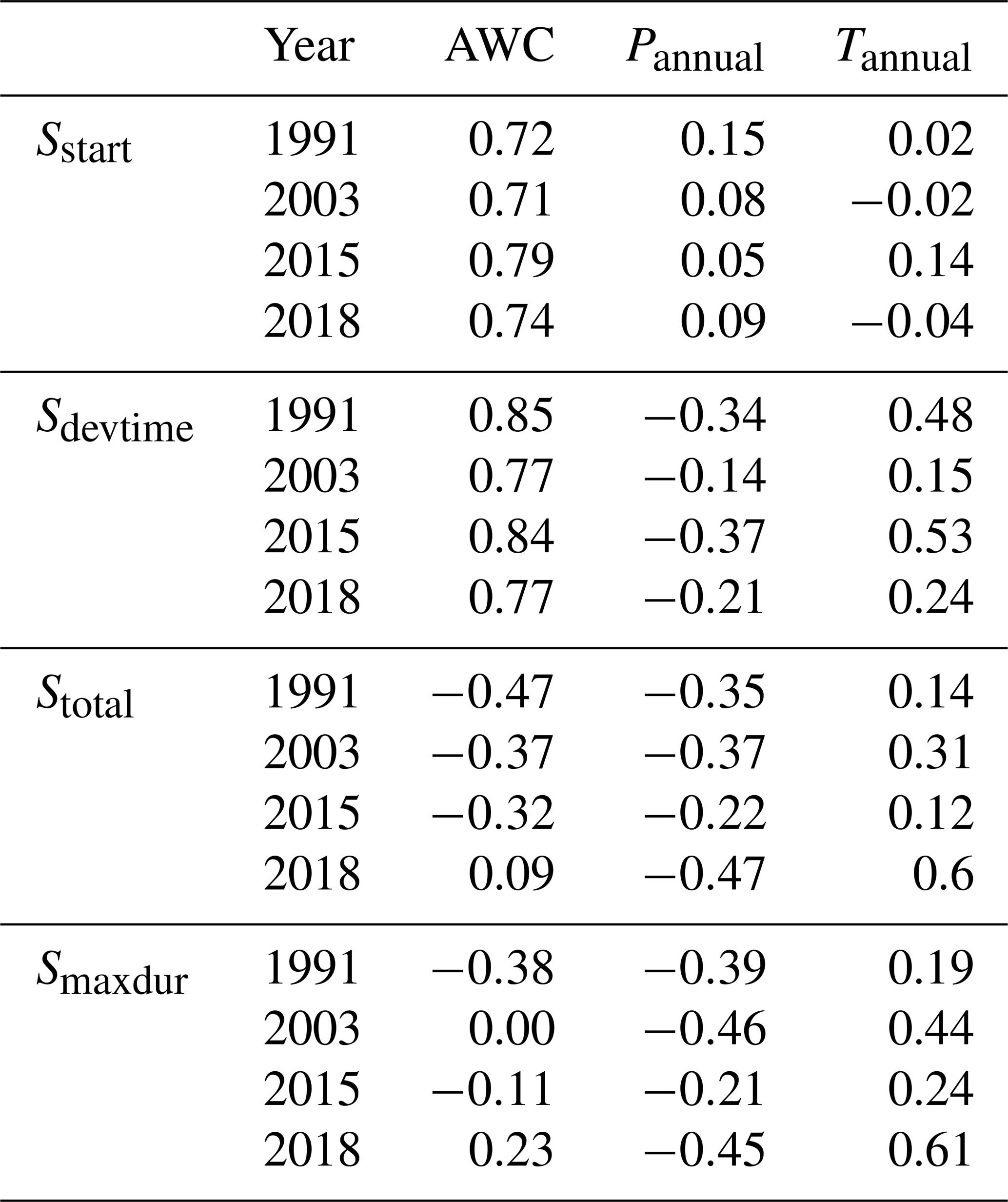
Figure 9 shows the meteorological anomalies during the development and annual maximum duration of SM stress (all events of all years combined, but separated based on the length of the development time and duration, i.e., shorter or longer than 30 d). During the development of SM stress, P_perc,dev was almost always anomalously low, whereas T_perc,dev and especially E_perc,dev were often anomalously high, especially for the more quickly developing events (Fig. 9a). The distributions of E_perc,dev and especially T_perc,dev show a larger spread than the distribution of P_perc,dev. The latter implies that especially P needed to be anomalously low for SM stress to develop, whereas E and T could be more variable during the development. During the annual maximum duration SM stress event, P_perc,maxdur was again generally anomalously low (Fig. 9b). However, P_perc,maxdur shows a larger variation and spread and was generally higher than P_perc,dev, particularly for the shorter events. T_perc,maxdur and E_perc,maxdur show contrasting anomalies, where T was often above normal and E often below normal during the annual maximum duration SM stress event, especially for the events with a longer duration.

3.3 Sensitivity to the parametrization of S_rootzone and used identification method

The sensitivity analyses reveal that the parameterization of S_rootzone affected the total number of agricultural grid cells that reach SM stress (Fig. S6). However, this parameterization had little effect on the relative ordering among drought years, i.e., independent of the chosen S_rootzone parameterization, the most severe drought years, in terms of the number of grid cells that reached SM stress, were 2018 and 2003, followed by 2015 and 1991. Furthermore, differences in the number of grid cells that reached SM stress was small between results derived from simulations with a soil-based S_rootzone and a soil-based S_rootzone constrained at 1 m depth. Larger differences were found among results derived from simulations with a S_rootzone that had a fixed AWC. More distinct were differences between SM stress and SM drought. Most grid cells reached an anomalously low state at least once in a calendar year, independent of the parameterization of the root zone, whereas SM stress shows more variation between individual years.

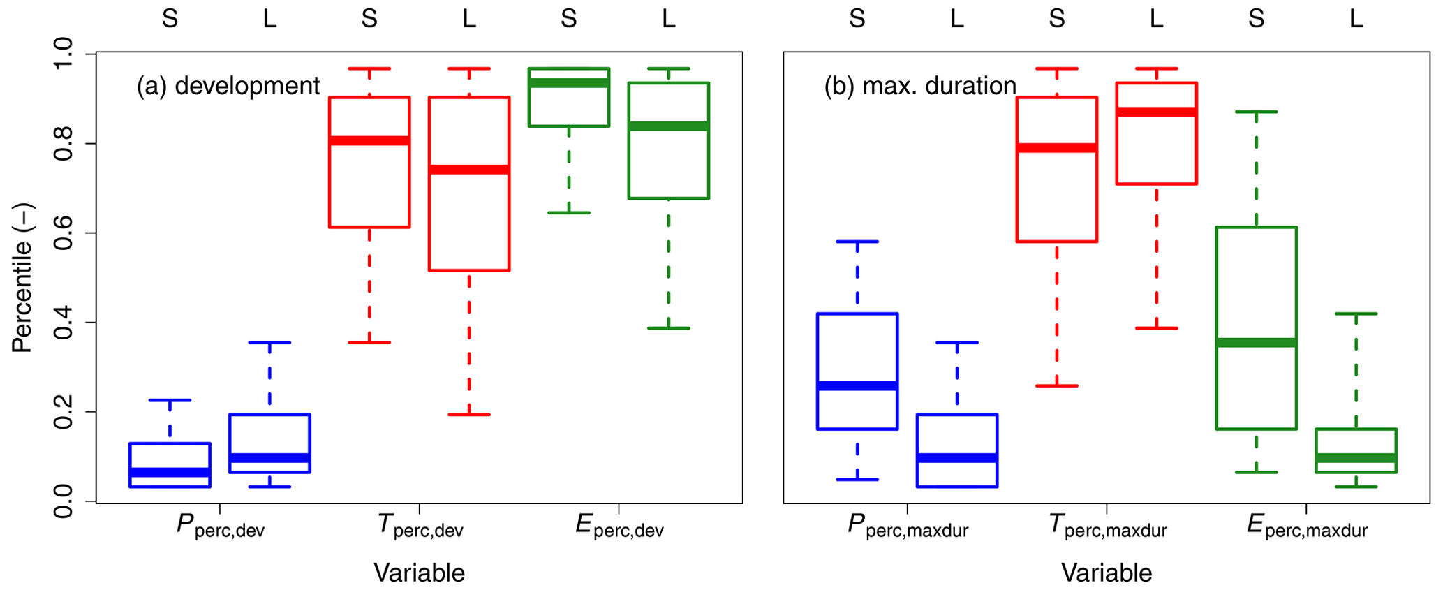
Figure 9 Meteorological anomalies (percentiles) of precipitation (P_perc), temperature (T_perc), and actual evapotranspiration (E_perc) during (a) the development (dev) and (b) the annual maximum duration (maxdur) of SM stress. Results are split into SM stress episodes with a relatively short (S; < 30 d) and relatively long (L; ≥ 30 d) development times (ratio S $/$ L is $\mathrm{40}/\mathrm{60}$ %) and maximum duration (ratio S $/$ L is $\mathrm{67}/\mathrm{33}$ %). The box shows the 25th, 50th, and 75th percentile, and the end of the whiskers shows the 5th and 95th percentile.

The probability of reaching SM stress was affected by the AWC of the root zone for results derived from soil-based S_rootzone parameterizations (Fig. S7). In case the AWC was fixed, its control was obviously removed, and the climatological setting (P_annual and T_annual) had a larger influence. Especially results derived from a fixed AWC of 200 mm show a clear distinction, where SM stress had a higher probability to develop in relatively dry and warm regions, with a shift in probability functions towards wetter and colder regions during prominent drought years. For SM drought, there was little to no relationship between the probability of reaching SM drought for at least 1 d in a certain year and the considered controls, given that most grid cells reach SM drought for at least 1 d in most years.

The parameterization of S_rootzone also affected other SM stress characteristics (S_start, S_devtime, S_total, and S_maxdur) in their overall magnitude (Fig. S8). However, the relative ordering in the severity of prominent drought years, according to those characteristics, was often preserved. The distributions of S_start were comparable between soil-based S_rootzone parameterizations, whereas S_start is generally earlier for root zones with a fixed AWC of 100 mm and later for root zones with a fixed AWC of 200 mm (as expected). More pronounced was the difference between S_start of SM stress and SM drought, as daily SM anomalies reached a below-normal state for the first time much earlier in the year. S_devtime also varied, depending on the S_rootzone parameterization. As expected, SM stress developed faster for root zones with the AWC fixed at 100 mm, slower for root zones with the AWC fixed at 200 mm, and somewhere in between these ranges for soil-based parameterizations of the root zone (with again little difference between the two soil-based parameterizations). The ordering of the box plots among prominent drought years was comparable among S_rootzone parameterizations, despite 2003 developing relatively fast with the AWC fixed at 100 mm and 2015 developing relatively slowly with the AWC fixed to 200 mm. The distributions of the S_total and S_maxdur in different drought years were comparable among S_rootzone parameterizations. More notable is the difference with SM drought, i.e., SM was much longer (continuously) in an anomalously low state compared to the time in SM stress. The ordering of most severe drought years, according to duration of the drought, remained the same and is comparable to the ordering of SM stress, with one notable difference for the drought of 2003 derived from a fixed S_rootzone parametrization with an AWC of 200 mm, which lasted relatively long compared to other drought years.

S_start of SM stress derived from the simulations with a soil-based root zone parameterization was most strongly related to the AWC and less to the climatological setting (Fig. S9). When the AWC of S_rootzone was fixed, S_start positively correlated with P_annual and negatively with T_annual, i.e., SM stress started later in wetter and colder regions. This is different for SM drought (anomaly) for which the first day is positively correlated with P_annual and negatively correlated with T_annual. S_devtime of SM stress is most strongly correlated to the AWC and less strongly correlated to the climatological setting for soil-based root zone parameterizations. For root zone parameterizations with a fixed AWC, no correlations with P_annual and a negative correlation with T_annual (some years) were found. S_total and S_maxdur of SM stress were only weakly correlated to the AWC of the root zone, whereas the total and maximum duration of SM drought showed a strong positive correlation with the AWC. In other words, SM droughts lasted much longer in thicker root zones with a higher AWC, whereas these root zones were not necessarily in a longer state of SM stress. S_maxdur and S_total of SM stress were further correlated to P_annual and T_annual, especially for (shallow) root zones with a fixed AWC, whereas S_maxdur and S_total of SM drought generally showed lower correlations with P_annual and T_annual.

4 Discussion

Our first objective was to characterize the occurrence, development time, and persistence of simulated past soil moisture (SM) stress events. Results revealed a large temporal variability in the number of grid cells that reach SM stress in a certain year (Fig. 6). The most severe SM stress years were 2003 and 2018, during which up to 89 % of the agricultural grid cells reached SM stress. These percentages of grid cells were found to be (slightly) different, depending on the parameterization of S_rootzone (Fig. S6), implying differences between, for example, shallow rooting crops with limited access to water and deeper rooting crops with a larger water availability. Nevertheless, the ordering of most severe drought years was not affected by the parameterization of the root zone, i.e., 2003 and 2018 were always characterized as most severe in terms of the number of grid cells that reached SM stress. Previous studies already showed that 2003 was an extreme drought year within and around the study region (e.g., Ionita et al., 2017). Results of this study imply that the recent 2018 event was comparable to 2003 in terms of the number of grid cells that reach SM stress. However, even during these most severe drought years, SM stress did not develop for some of the agricultural grid cells (unless a root zone with a fixed AWC of 100 mm was used), either because of (1) local variations in meteorological conditions (e.g., local rains storms) or (2) root zone soils having a large enough storage capacity that acted as a buffer during dry conditions. This illustrates that, even during the most extreme drought years, regional differences can occur. The factors that control these differences, i.e., the occurrence of local rainstorms and differences in soil characteristics, can be spatially heterogeneous. The latter implies that regional agricultural drought assessments and monitoring should occur at a relatively high spatial resolution to be able to capture these differences.

A large variability in the development time of simulated SM stress was found (Fig. 8b). SM stress could develop in less than 10 d, e.g., in shallow root zones with a low available water-holding capacity (AWC). This is faster than the minimum development time of 30 d used to identify rapid-onset (flash) droughts in, e.g., Christian et al. (2019). On the other hand, it could also take a lot longer (over 4 months) for SM stress to develop. This slower development matches better with the traditional description of drought being a slowly developing (creeping) phenomena (Wilhite and Glantz, 1985). The above-stated ranges in the development time were reduced when the starting point of SM stress development was set to a level lower than field capacity (Fig. S10), implying that it is important to keep track of partially depleted soil moisture stores that can be a precursor to more rapid development. The sensitivity analyses revealed that fixing S_rootzone reduces the variability in development time; however, also showing the distinct differences between root zones with a relatively low and high storage capacity, which is indicative for differences between shallow and deep rooting crop species. Furthermore, the relative ordering of drought years in terms of their S_devtime was often the same, besides few exceptions, which relates to specific differences in the configuration of meteorological dry spells and whether they caused SM stress under different S_rootzone parameterizations. Overall, the large differences in development time suggest that different types of forecasting systems could be suitable for predicting the development of SM stress, medium-range weather forecasts for quickly developing events, and more long-term meteorological forecasts for slower developing episodes.

The persistence of SM stress (total days and maximum duration) varied strongly between years and grid cells (Fig. 8c, d). The results of this study showed that the total days and maximum duration of SM stress was generally highest in 2018, making this event more severe than earlier (recent) benchmark events, such as 2003. The long nature of the drought of 2018 was also found in a recent study for Switzerland, the country directly south of our study region, in Brunner et al. (2019). The ordering of most extreme drought years according to duration was often found to be independent of the parameterization of S_rootzone or whether SM stress or drought was analyzed (Fig. S9). On the other hand, distinct differences in duration were found, especially between SM stress and drought, i.e., SM was generally much longer in an anomalously low state compared to the time when it was in a state of SM stress. This can be partially explained by the fact that SM can be anomalously low without being severely depleted, especially towards the end of the year, after a severe drought year, when SM stores are not completely filled to field capacity again (as would normally be the case). We also found that the annual maximum duration and total time of SM stress never exceeded 6 months, and most of the root zones reached field capacity again each year before the start of the new growing season. Thus, SM stress was never a multi-year phenomenon for the considered agricultural grid cells. SM droughts, on the other hand, can last longer and could more easily persist into the next year.

Our second objective was to investigate the dominant controls on the probability, development time, and persistence of SM stress. Both probability and development time were most strongly related to the AWC of the root zone and less to the climatological setting (Fig. 7; Table 1). SM stress was generally more likely to develop, and it evolved faster and earlier in the year in shallow root zones with a lower AWC. These findings are in line with results for the 2012 flash drought in the US presented by Otkin et al. (2016), where anomalous soil moisture conditions generally first appeared in the topsoil layer (lower AWC) and only later in the entire soil layer (higher AWC). Results also confirm that AWC of the root zone is an important factor for determining the vulnerability to agricultural drought, as was also stated in, e.g., Wilhelmi and Wilhite (2002). Here, it is important to state that AWC is not only a soil parameter but also encompasses differences between, for example, a shallow or deep rooting crop, as was exemplified by the differences between the two root zone parameterizations with a fixed AWC found in the sensitivity analyses (Figs. S6, S8). Finally, these results imply that agricultural drought assessments purely based on meteorological proxy indicators should be interpreted with care as most meteorological proxy indicators do not consider differences in root zone soil characteristics.

The persistence of SM stress was only weakly correlated with the AWC of the root zone and more strongly with the climatological setting (Table 1), especially when considering a parameterization of S_rootzone with a fixed AWC (Fig. S9). The reason for the overall weaker correlations with the AWC might be related to the different mechanisms that govern the persistence of SM stress in different types of root zones. In root zones with a low AWC, SM stress can develop rather quickly. However, the total deficit that can build up is limited, and only a small rainfall event is enough to alleviate SM stress conditions. In root zones with a high AWC, larger SM deficits can potentially develop. However, this development takes longer, and the SM stress threshold is only exceeded towards the end of the growing season, after which further development is limited because of lacking evapotranspiration. The most persistent SM stress events might, therefore, occur for root zones with an intermediate AWC. In these root zones, SM stress can develop reasonably fast but can also build up a large enough deficit that can endure some smaller rainfall events. This is different for the duration of SM drought (anomaly), which is positively correlated with the AWC of the root zone, i.e., SM droughts tend to last longer for root zones with a higher storage (Fig. S9). A reason for this is that SM (anomaly) time series derived from root zones with a larger AWC often exhibit a much more gradual behavior, whereas SM (anomaly) time series derived from root zones with a smaller AWC are often flashier. Another reason for this is that it can take much longer for root zones with a larger AWC to reach a level of field capacity towards the end of the year (normal conditions) after a prolonged meteorological dry spell.

The third objective of this study was to portray the meteorological anomalies during (the development of) simulated SM stress. During the development, especially the precipitation needed to be anomalously low, particularly during the more rapidly developing events (Fig. 9a), suggesting that lacking precipitation was the most important prerequisite for SM stress to develop. However, air temperature and evapotranspiration were also often higher than normal during the development of SM stress, implying an enhancing (compound) effect of these variables (see also Manning et al., 2018), especially during rapid onset events. During the annual maximum duration SM stress events, precipitation was often below normal as well, especially for the longer events (Fig. 9b). However, precipitation anomalies during the maximum duration events were not as extreme as during the development, possibly because SM only needed to remain in a steady state condition of SM stress, rather than having to decline from field capacity to a level of SM stress. Temperature and simulated evapotranspiration show contrasting anomalies during the annual maximum duration SM stress events, with temperature generally being above normal and simulated evapotranspiration generally being below normal, particularly during the longer events. The reason for these contrasting anomalies might be related to a different energy partitioning of heat fluxes during SM stress (described in, e.g., Seneviratne et al., 2010). During SM stress, simulated evapotranspiration was anomalously low because of the water stress for vegetation that causes plants to limit their evapotranspiration assumed in the model. The incoming solar radiation that is normally consumed by evapotranspiration (latent heat flux) is now used to warm up the soil and lower atmosphere (sensible heat flux), possibly explaining the above-normal temperatures during SM stress (Miralles et al., 2014). This energy partitioning during SM stress, and the resulting contrasting temperature and evapotranspiration anomalies, highlights that agricultural drought assessments derived from meteorological proxy indicators based on potential evapotranspiration should be interpreted with care.

Our regional assessment of SM stress is subject to inaccuracies, challenges, and assumptions, which is common for these kinds of analyses. A source of the inaccuracies relates to the modeling of SM. Previous studies showed that the physically based TRAIN model was able to provide a good temporal representation of soil moisture over agricultural fields (e.g., Stork and Menzel, 2016). However, it is important to bear in mind that the studied results are regional model simulations for specific soil and land use parameterizations that can be different from the heterogeneous real world. An evaluation of the simulated hydrological fluxes with observed streamflow suggests that TRAIN provides a reasonable estimation of the water balance and its variability (Figs. 5 and S2–S5). However, there are other models, model structures, and model parameterizations to simulate soil moisture, implying a dependency between the used model (parameterization) and the results (shown in, e.g., Samaniego et al., 2018; Zink et al., 2017). The latter studies use ensembles of different models or different model parameterizations to consider model- or parameter-related uncertainties, which is beyond the scope of the current study.

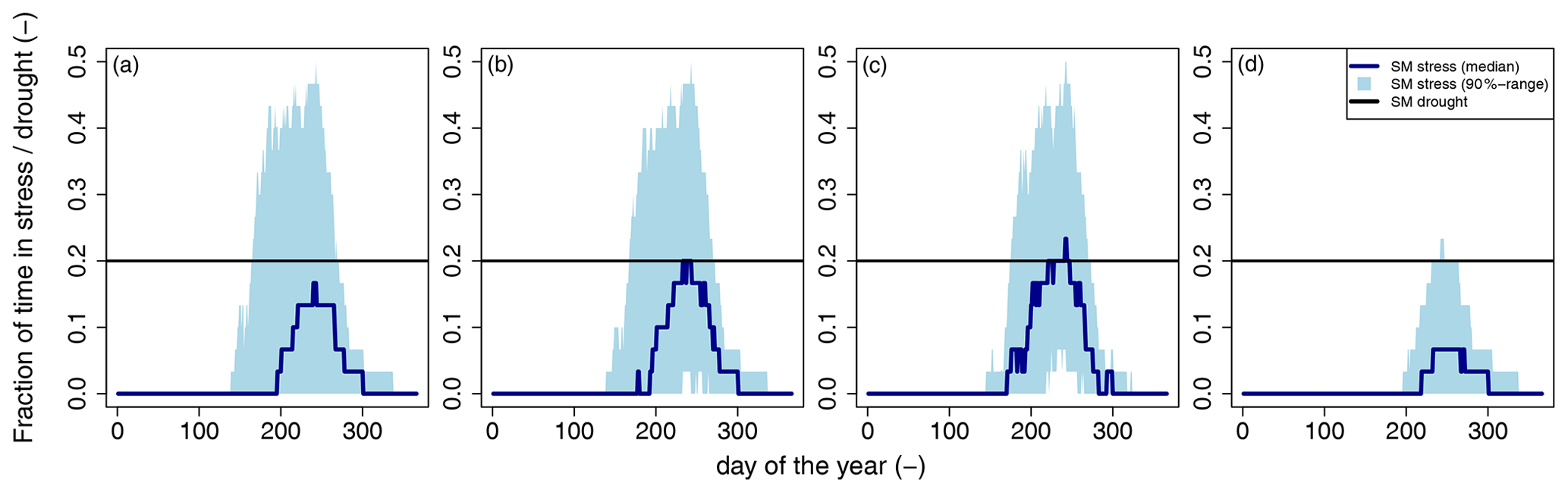
Figure 10 Temporal variation in SM stress and drought occurrence frequency derived for each day of the year from results of different parameterizations of the root zone, namely (a) soil based, (b) soil based constrained at 1 m depth, (c) S_rootzone with a fixed AWC of 100 mm, and (d) S_rootzone with a fixed AWC of 200 mm.

Another source of inaccuracies stems from the data used to set up and force the model. A challenge was the interpolation of several different meteorological variables over a rather complex terrain which is prone to biases, especially for variables such as wind speed. Another challenge was the spatially accurate representation of the root zone soil, both in terms of the interpolation of heterogeneous soil and land use characteristics and in the parameterization of the rooting depth. The interpolation of soil and land use characteristics was based on the majority class within a 1 km grid cell. However, each grid cell can still exhibit a large variability in soil and land use characteristics, implying that the simulated SM dynamics might not be representative for the entire grid cell. The parameterization of the rooting depth of each grid cell was further based on soil characteristics, which is a procedure that is often used to parameterize regional models. However, roots do not necessarily utilize the water in the entire soil column, and rooting depth depends on other factors, such as the type of crop. For example, a soil might have a maximum rooting depth of 1 m; however, if a shallow rooting crop species is grown in this soil, roots may not have access to all water. A sensitivity analyses revealed that derived results change depending on the used parameterization. Differences in (controls on) simulated SM stress characteristics are small between a soil-based root zone and a soil-based root zone constrained to 1 m depth, implying that the latter depth constraint does not have a great impact on simulated SM stress characteristics. The differences were larger when the volume of the AWC of the root zone was constrained to a fixed value, i.e., mimicking shallow and deeper rooting crop species with lower and higher water availabilities, respectively. An option not considered was a climate-based parameterization of the root zone, which works with the hypothesis that the (catchment average) size of the AWC of S_rootzone (dynamically) develops to deal with meteorological droughts of certain return periods (e.g., 10 years). Various studies show improved model performances for a selection of catchments when defining the root zones in such a way as opposed to a soil-based definition (e.g., de Boer-Euser, et al., 2016). The reason why we did not apply this parameterization in our study is that (1) we focus on annual agricultural crops that are harvested every year and, thus, do not have the opportunity to gradually adapt their root zones over time, and (2) such analyses require a study with a different scope. In the end, an accurate spatiotemporal representation of the root zone, considering the influence of soil-, climate- and crop-specific characteristics (as well as their interactions), remains an important challenge. With the sensitivity analyses, we cover four possible scenarios, but different assumptions might apply, depending on the scope of the study.

The soil-based parametrization of the root zone, the variability in soil, and land use characteristics within a single grid cell and possible biases in interpolated meteorological variables mean that results might not always be accurate for a specific grid cell or for a single agricultural field located within this grid cell. However, by analyzing a large sample of grid cells and by including a sensitivity analyses to the parameterization of the root zone, we cover a large number of combinations of root zone characteristics and climatological settings that occur within the study region (Fig. 1). Lessons learned from these large samples, for example, about the relationship between SM stress characteristics and soil or climate properties (e.g., Fig. 7; Table 1), provide insights that might be relevant for smaller (local) scales within the study region; however, this is only the case when the modeling assumptions, for example, behind the parameterizations of S_rootzone, apply. Here, the most suitable assumption can vary, depending on the studied crop, for example, whether the crop being studied makes full use of all plant-available water in the root zone soil or whether the crop being studied is a shallow rooting crop that only uses of part of it.

An assumption that was made in this study relates to the definition of SM stress. We characterized periods of SM stress (absolute) rather than SM drought (anomaly). We used one fixed threshold of 30 % of the AWC to define SM stress. This threshold is in line with the indicative threshold for potential SM stress used by the German Weather Service (DWD, 2018). However, it should be noted that this threshold, and the relationship between the degree of SM stress and the amount of available water left in the root zone, varies depending on, for example, crop species, climatological conditions, and soil type (Allen et al., 1998). Notwithstanding these assumptions, we believe that, from an agricultural drought impact perspective, the used definition of SM stress is more closely related to actual water stress experienced by plants than an anomaly-based definition. This is especially so because SM anomalies can be significantly different from SM stress, and below-normal anomalies often correspond to situations with sufficient soil moisture (Fig. 10). SM stress often still relates to an anomalously low state that develops and persists during periods with below-normal precipitation (Fig. 9). However, SM stress also incorporates temporal variability, with an increased occurrence during the growing season and a limited occurrence during the non-growing season, whereas SM drought occurs equally distributed over the year (Fig. 10). Furthermore, the rareness of SM stress is affected by the plant-available water-holding capacity of the root zone soil and the climatological setting as revealed by, for example, the ranges in Fig. 10 or the difference between Fig. 10c and d, whereas this is not the case for SM drought. On the other hand, it should be noted that derived SM stress characteristics are more sensitive to modeling assumptions and uncertainties. SM stress characteristics derived from simulations using different parameterizations of the root zone reveal more variation (Fig. 10) but, therefore, also a higher degree of disagreement on whether SM stress was reached (Fig. S11a). Soil moisture anomalies show a higher degree of agreement, i.e., results are more robust and much less sensitive to the (uncertainties in) parameterization of the root zone (Fig. S11b). Overall, the definition of SM stress used in this study might be applicable in other regions or for other research purposes, for example, those that aim to investigate changes in agricultural drought vulnerability under climate change.

5 Conclusion

Meteorological droughts cause soil moisture levels to decline. Diminished root zone soil moisture can largely affect agricultural productivity, as crops might experience soil moisture stress. In this study, we investigated the characteristics of simulated past soil moisture stress events across the agricultural regions of southwestern Germany and their relationship with soil and climate variables. The total agricultural area that reached soil moisture stress conditions was found to vary strongly among the years and was highest in 2003 and 2018. In terms of the development time, 2003 was not much different from 2018. In both years, development time varied from as little as 10 d to over 4 months. What made 2018 distinctively different from 2003 was the generally longer total time and maximum duration of simulated soil moisture stress, highlighting the extraordinary severity of the most recent event studied.

Both the occurrence and development time of soil moisture stress were found to be strongly related to the available water-holding capacity of the root zone and not so much to the climatological setting. That is, when we assume roots can make use of all available water in the root zone column by being either constrained or not constrained at a depth of 1 m. When we assume root zones of fixed sizes, the influence of the climatological setting increases, yet the difference between a shallower rooting crop (lower AWC) and a deeper rooting crop (higher AWC) remains. Thus, the above findings stress the importance of considering differences in root zone storage characteristics for agricultural drought assessments and monitoring and early warning, independent of whether these differences in storage are related to the difference in soil or crop species. Nonetheless, a major challenge remains with respect to the accurate spatiotemporal characterization of the root zone soil that considers (the interactions between) soil, climatological, meteorological, and crop-specific factors.

Results of this study further imply that below-normal precipitation was the most important reason for soil moisture stress to develop. However, the often above-normal anomalies of temperature and, especially, simulated evapotranspiration during development suggest an augmenting effect of these variables. During soil moisture stress, temperature anomalies were found to often be above normal, which contradicted with the often below-normal simulated evapotranspiration anomalies. These contrasting anomalies of temperature and evapotranspiration imply that agricultural drought assessments derived from meteorological proxies based on potential evapotranspiration should be interpreted with care. The same is the case for agricultural assessments based on soil moisture anomalies, as below normal anomalies were found to not necessarily correspond to a situation of soil moisture stress, especially for periods outside the growing season. In addition, the sensitivity analyses revealed that SM drought characteristics, and controls on these characteristics, can differ significantly from (controls on) SM stress characteristics. Overall, the approach presented in this study of directly characterizing simulated soil moisture stress events for agricultural drought assessments might, in some cases, be a suitable alternative to approaches based on meteorological proxies or soil moisture anomalies.