A multi-sourced assessment of the spatiotemporal dynamics of soil moisture in the MARINE flash flood model

The MARINE (Model of Anticipation of Runoff and INundations for Extreme events) hydrological model is a distributed model dedicated to flash flood simulation. Recent developments of the MARINE model are explored in this work. On one hand, transfers of water through the subsurface, formerly relying on water height, now take place in a homogeneous soil column based on the soil saturation degree (SSF model). On the other hand, the soil column is divided into two layers, which represent, respectively, the upper soil layer and the deep weathered rocks (SSF–DWF model). The aim of the present work is to assess the accuracy of these new representations for the simulation of soil moisture during flash flood events. An exploration of the various products available in the literature for soil moisture estimation is performed. The efficiency of the models for soil saturation degree simulation is estimated with respect to several products either at the local scale or spatially distributed: (i) the gridded soil moisture product provided by the operational modeling chain SAFRAN-ISBA-MODCOU; (ii) the gridded soil moisture product provided by the LDAS-Monde assimilation chain, which is based on the ISBA-A-gs land surface model and assimilating satellite derived data; (iii) the upper soil water content hourly measurements taken from the SMOSMANIA observation network; and (iv) the Soil Water Index provided by the Copernicus Global Land Service (CGLS), which is derived from Sentinel-1 C-SAR and ASCAT satellite data. The case study is performed over two French Mediterranean catchments impacted by flash flood events over the 2017–2019 period. The local comparison of the MARINE outputs with the SMOSMANIA measurements, as well as the comparison at the basin scale of the MARINE outputs with the gridded LDAS-Monde and CGLS data, lead to the following conclusion: both the dynamics and the amplitudes of the soil saturation degree simulated with the SSF and SSF–DWF models are better correlated with both the SMOSMANIA measurements and the LDAS-Monde data than the outputs of the base model. Finally, the soil saturation degree simulated by the two-layers model for the deep layer is compared to the soil saturation degree provided by the LDAS-Monde product at corresponding depths. In conclusion, the developments presented for the representation of subsurface flow in the MARINE model enhance the soil saturation degree simulation during flash floods with respect to both gridded data and local soil moisture measurements.

1 Introduction

The risk associated with flash flood events is of growing importance, in particular in the Mediterranean area (Payrastre et al., 2011; Ruin et al., 2014; Suárez-Almiñana et al., 2020). Extreme precipitation events are expected to increase both in frequency and amplitude in the context of a changing climate (IPCC, 2014). In particular, modeling systems for short-term predictions represent valuable tools for decision-making and the organization of emergency systems. The accuracy of modeling tools available for operational purposes therefore have increasing stake. The main variable of interest for flood simulations at the catchment scale is usually the discharge variable, which integrates all the processes taking place at the subsurface and the surface of the catchment. However, surface runoff, itself controlled by soil infiltration rates, is shown to exacerbate both human and material risks during extreme events (Vincendon et al., 2010). The representation of soil processes in the models is thus a key factor for flash flood simulation (Berthet et al., 2009).

Several mechanisms generate the partition between infiltration and surface runoff. Surface runoff can happen when rainfall intensity exceeds the maximum infiltration rate of the soil (infiltration excess) or when the precipitation volumes exceed the storage capacity of the soil (saturation excess). Then, the generation of surface runoff directly relies on the water content of the subsurface. Within the subsurface, both vertical infiltration flows and lateral transfers take place. These flows are controlled by the physical characteristics of the porous media, such as its hydraulic conductivity or its capacity at saturation. In addition, preferential flows happen through macropores or fractured aquifers.

Among the variety of models developed for flash flood simulation, the physical processes taking place in the subsurface are represented based on various formalisms. While some models do not consider the infiltration flow at the scale of the flood event (Berthet, 2010), other models represent the soil column as one or several reservoirs with different degrees of refinement for the representation of the physics of the processes. Vertical infiltration flow can be parameterized through simple calibrated relations, in particular through linear relations (Perrin et al., 2003) or exponential relations. Other approaches apply a more physically oriented representation of vertical infiltration in the subsurface based on the Richard's equation. The lateral transfers in the subsurface are generally represented in flood models through kinetic wave equations. In this case, the parameters controlling the infiltration rates are either calibrated (Roux et al., 2011) or extracted from pedological and geological descriptions (Bouilloud et al., 2010; Vincendon et al., 2010; Vannier et al., 2014).

Various works quantify the sensitivity of different models to the subsurface parametrization (Tramblay et al., 2010; Garambois et al., 2015b; Douinot et al., 2017; Edouard et al., 2018; Lovat et al., 2019). They show that uncertainties in the representation of infiltration processes strongly impact both discharge and surface runoff simulations during flood events. In addition, both the lack of soil description and the uncertainties associated with soil moisture (SM) estimations lead to a hazardous validation of the model outputs (Manus et al., 2009). In this work, an exploration of the various products available in the literature for soil moisture estimation is performed. Three main types of data can be used to estimate the efficiency of hydrological models regarding the soil moisture. (i) Local ground measurements provide locally accurate estimations of soil moisture at shallow depths. Several studies have demonstrated that local soil moisture measurements are representative of relatively large areas and hence they can be compared to spatially distributed simulation outputs around the point of measurement (Brocca et al., 2009; Tramblay et al., 2010). In particular, the SMOSMANIA network consists of 21 ground point measurements in southern France (Calvet et al., 2007; Albergel et al., 2009; Parrens et al., 2012). (ii) Land surface and distributed hydrological models provide gridded information over a large area and they can provide information for different depths and different variables. For example, the SAFRAN-ISBA-MODCOU modeling chain (Habets et al., 2008) as well as the LDAS-Monde products (Albergel et al., 2017) are both based on the ISBA surface scheme (Noilhan and Planton, 1989; Noilhan and Mahfouf, 1996) implemented in the SURFEX platform (Masson et al., 2013). (iii) Satellite imagery provides valuable spatially distributed data. Different remote sensing techniques have been developed for obtaining soil moisture from satellite measurements. Microwave remote sensing provides a means to quantitatively describe the water content of a shallow near-surface soil layer. However, the variable of interest for applications in short- and medium-range meteorological modeling and hydrological studies over vegetated areas is the root-zone soil moisture, which controls plant transpiration but is not directly observable from space. Since the near-surface soil moisture is related to soil moisture through diffusion processes, assimilation algorithms may allow its retrieval. Estimation of the root-zone soil moisture from intermittent remotely sensed surface data has focused on the assimilation of such data into land surface models. Many studies now also suggest that constraining those land surface models using various types of earth observations, including vegetation-related earth observations, may lead to a better representation of the root-zone soil moisture (Bolten et al., 2009; Pezij et al., 2019; Wagner et al., 2012). In addition, simplified approaches (e.g., Soil Water Index) have also been developed for obtaining root-zone soil moisture.

The MARINE model (Model of Anticipation of Runoff and INundations for Extreme events) is a distributed, physically based hydrological model (Roux et al., 2011). MARINE is used by operational French flood forecasting services for flood risk assessment. The recent developments of the MARINE model proposed by Douinot et al. (2018) lead to an improved representation of the subsurface flows. On one hand, transfers of water through the subsurface, which formerly relied on water height, now take place in a homogeneous soil column based on the soil saturation degree (SSF model). On the other hand, the soil column is divided into two layers, which represent, respectively, the upper soil layer and the deep weathered rocks (SSF–DWF model). These developments enhance the degree of refinement of the soil physics described in the model. The impacts of this representation of the subsurface on the water discharge have been extensively studied by Douinot et al. (2018). However, their influence on the spatial dynamics of soil saturation degree has not yet been explored.

Thus, this work aims to assess the impacts of the developments proposed by Douinot et al. (2018) to include a physically oriented soil representation in MARINE with respect to the soil saturation degree (SSD) dynamics during flash flood events. The efficiency of the models for SSD simulation is estimated with respect to several soil moisture products: (i) the gridded soil moisture product provided by the operational modeling chain SAFRAN-ISBA-MODCOU, available at the 8 km × 8 km spatial resolution (Habets et al., 2008); (ii) the gridded soil moisture product provided by the LDAS-Monde assimilation chain, based on the ISBA-A-gs land surface model and assimilating high-resolution spatial remote sensing data (Albergel et al., 2017; Calvet et al., 1998) (this work uses the version of LDAS-Monde at the 2.5 km × 2.5 km spatial resolution); (iii) the hourly soil water content measurements taken from the SMOSMANIA observation network (Calvet et al., 2007); and (iv) the Soil Water Index provided by the Copernicus Global Land Service (CGLS), available at the 1 km × 1 km resolution and derived from Sentinel-1 C-band SAR and ASCAT satellite data (Bauer-Marschallinger et al., 2018a). The comparison between the MARINE output for SSD dynamics and these three sources of data is performed both at the local point measurement scale and at the catchment scale. These products represent valuable indicators of the spatiotemporal dynamics of soil moisture at various scales.

In Sect. 2, the MARINE model, its new developments for the soil model, and also the study cases considered for this work are described. The soil moisture data used in this work are also presented in this section. In Sect. 3, the methods applied for the model setup and calibration and the comparison protocol are presented. The last section presents the results and discussion.

2 Model and data

2.1 The MARINE flash flood model

This section presents the base version of the MARINE model as proposed by Roux et al. (2011), together with the two advanced versions of the model implemented by Douinot et al. (2018) for soil process descriptions. Figure 1 summarizes the main state variables and flux regarding soil processes for the three versions of MARINE.

Figure 1 Summary of the main state variables and flux regarding soil processes for the three studied versions of MARINE: the base model (BM), the subsurface flow model (SSF), and the coupling of the SSF and deep water flow models (SSF–DWF). The two fluxes introduced in the SSF–DWF are colored in red. Each column represents the soil column for one grid cell of the model. h stands for water height in the soil layer and θ stands for the SSD of the layer. For the SSF–DWF model, the surf and deep subscripts are used to describe the upper soil layer and the deep soil layer, respectively.

2.1.1 Base model (BM)

The MARINE model is a distributed, physically based hydrological model (Roux et al., 2011). MARINE consists of three main modules. First, precipitation is separated between surface runoff and infiltration using the Green and Ampt model. Then, the subsurface flows are represented using an approximation of Darcy's law. Finally, the overland and river fluxes are simulated using the Saint-Venant equations simplified with kinematic wave approximation. The connections between the model components are extensively described in Roux et al. (2011). Based on sensitivity analyses of the model, five parameters are calibrated in MARINE for the representation of the soil and the surface: the multiplier coefficient for soil depth maps (C_z), the multiplier coefficient for the spatialized saturated hydraulic conductivity used in lateral flow modeling (C_kss), the multiplier coefficient for the spatialized hydraulic conductivity at saturation that is used in infiltration modeling (C_kga), and two friction coefficients for low- and high-water channels (Garambois, 2012).

2.1.2 The subsurface flow model (SSF)

This work uses the recent developments for the representation of the infiltration into the subsurface and the new two-layer soil model proposed by Douinot et al. (2018). These new models are integrated into PLATHYNES, the modeling platform of the French Service for Flood Forecasting (SCHAPI). In the MARINE base model, the transfers through the subsurface are a function of the water height (h). However, Douinot et al. (2018) show that expressing the subsurface flows as a function of the soil saturation degree (θ) of the cell instead of its water height appears to be a more appropriate choice to represent the activation of preferential paths. Thus, Douinot et al. (2018) define a new subsurface flow model (SSF) where the lateral flows are expressed as a function of the saturation degree of the cell.

2.1.3 The two soil layers model (SSF–DWF)

In the soil model initially implemented in MARINE (base model; see Sect. 2.1.1), the soil is represented by a single layer. Douinot et al. (2018) propose a version of the soil model for which two soil layers are defined, the so-called deep water flow model (DWF). With the DWF soil model, the soil column is subdivided by two layers that represent the “upper soil” part and the “weathered rock” part of the soil. This subdivision involves the definition of two new flows in addition to the lateral flow in the upper soil to represent (1) the flows between the cells and the flows towards the drainage network in the weathered rock, q_deep(h_deep), and (2) the vertical infiltration flow from the upper soil layer to the weathered rock layer, q_exch(θ_surf,θ_deep). In this DWF model, the depth of the upper layer is equal to the soil depth provided by the soil database and the deep layer has an uniform depth over the catchment. The deep layer depth is calibrated for each catchment.

The two developments made for the SSF and DWF models can be merged to create the SSF–DWF model for the subsurface flow representation in MARINE. In the SSF–DWF model, the soil column is separated into two layers. Vertical and lateral transfers in the upper soil layer are described as a function of the soil saturation degree. In the SSF–DWF model, the flows in the deep layer is defined as a function of the water height in the deep layer. The integration of the SSF–DWF model in MARINE necessarily implies the calibration of two additional parameters: (1) the ratio between of the hydraulic conductivity at saturation for the upper soil layer and the deep layer and (2) the uniform depth of the deep layer. Extensive descriptions of the DWF, SSF, and SSF–DWF model physics and parametrization are presented in Douinot et al. (2018). The above-named acronyms are consistent with the ones used by Douinot et al. (2018).

2.2 Studied cases

2.2.1 The Ardeche catchment in Vogue and the Orbieu catchment in Lagrasse

In this work, the study case is performed over two catchments located in southern France particularly prone to flash flood events: the Ardeche river in Vogue and the Orbieu river in Lagrasse. These two catchments were selected for this study because (i) numerous flash flood events have been inventoried over the last decade in these catchments (Gaume et al., 2009) and (ii) SMOSMANIA stations have been installed since 2006 in these catchments for real-time superficial soil water content measurements (see Sect. 2.3.4) (Calvet et al., 2007).

Figure 2 presents the geographic situation of these two catchments. The digital elevation model (DEM) from the French Geographic Institute (IGN-BD Topo©, http://geoservices.ign.fr, last access: 15 March 2021) at 25 m resolution is considered in this work. The pedological information is taken from the French National Institute for Agronomic Research (INRA) soil database for the Ardeche and Languedoc-Roussillon regions (Robbez-Masson et al., 2000). The land cover information is taken from the Corine Land Cover 2006 database (Aune-Lundberg and Strand, 2010).

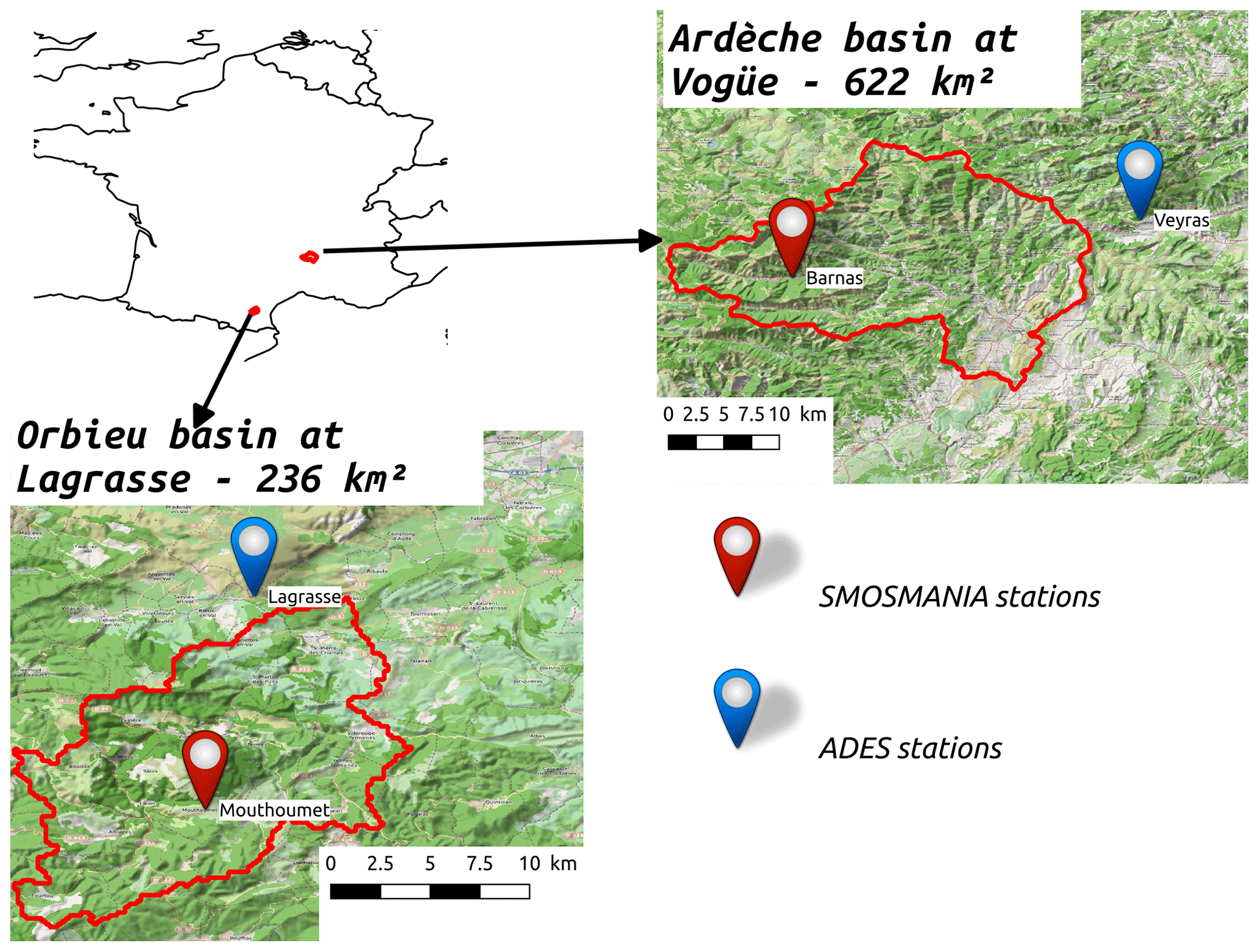
Figure 2 The two studied catchments located in southern France: the Ardeche river in Vogue and the Orbieu river in Lagrasse. Monitoring networks: soil water content (SMOSMANIA network stations) and the national groundwater ADES network stations (https://ades.eaufrance.fr/, last access: 15 March 2021).

The Ardeche catchment (622 km²; 193 to 1347 m a.s.l.) is located in the Cevennes region and exposed to intense precipitation events due to the convection of humid sea air masses over the Cevennes mountain slopes. The Orbieu catchment (236 km²; 135 to 807 m a.s.l.) is also exposed to Mediterranean extreme events, for example, the dramatic flood event of October 2018. The Ardeche catchment presents a mixed geology, with metamorphic rocks and schists on the upper part of the catchment and sedimentary plains downstream (source: http://infoterre.brgm.fr, last access: 15 March 2021). The land cover for the Ardeche catchment is mainly mixed forest, natural grasslands, and shrubs. The Orbieu catchment consists of a sedimentary area, mainly covered by arable land. Both catchments are minimally anthropized. The soil is 27 cm deep, on average, for the Ardeche catchment (between 5 and 50 cm) and 37 cm deep, on average, for the Orbieu catchment (between shallow and 73 cm). The soil texture is mainly sandy-loam for the Ardeche catchment, with silt deposits downstream, and mainly silt and silty-loam for the Orbieu catchment. Extensive geomorphological descriptions of these two catchments can be found in Adamovic et al. (2016); Douinot et al. (2018) and Garambois et al. (2015b).

2.2.2 The studied events

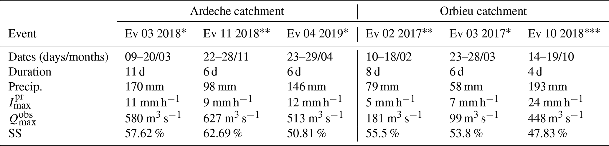
In this work, the ANTILOPE quantitative precipitation estimates (QPEs) are used for precipitation estimation (Champeaux et al., 2009). The ANTILOPE QPEs are based on a fusion between the radar data provided by the operational radar network ARAMIS (Tabary, 2007) and the measurements at rain gauges, spatialized by the kriging method. ANTILOPE QPEs are available at hourly time step and 1 km × 1 km resolution. The criticized observed discharges at the outlet of the two catchments are taken from the hydrometric French database (http://www.hydro.eaufrance.fr, last access: 15 March 2021). Table 1 presents the characteristics of the studied events.

Three flash flood events are considered for each catchment over the 2017–2019 period. This period is chosen because it corresponds to the period of availability of the LDAS-Monde at fine scale (2.5 km × 2.5 km resolution and 3 h time step) (Bonan et al., 2020). The heterogeneity of the studied events has to be noted; for the Orbieu catchment, the extreme event of October 2018 represents the historical maximum for this region, with well-known dramatic damage to infrastructure and populations. This flood has the characteristic of being extremely fast, with about 2 h between the precipitation peak and the discharge peak at the Lagrasse station. A very specific pattern of precipitation occurred during this event. The precipitation field was oriented along the main axis of the river, resulting in intense and devastating surface runoff (Caumont et al., 2020). This response time appears to be faster than the response time regularly considered for this station (about 5 h). In contrast, the two other events considered for the Orbieu catchment, in February and March 2017, represent relatively small floods, with return periods of 5 years and 2 years, respectively. For the Ardeche catchment, autumn 2018 presented a series of intermediate flood events. For this period, the damages were mainly induced by the duration of the flooding period. During the event defined from 22 November 2018 to 28 November 2018, the precipitation amounts do not represent extreme values. However, flood damages were noticed during this period. Consequently, this event is considered an important flood event. In addition, different hydrological responses can by distinguished for the spring or autumn seasons due to different soil and vegetation conditions or possible snow contribution. This variety in the structures of the six events considered for this study represents both a robustness guaranty and a challenge for the modeling exercise.

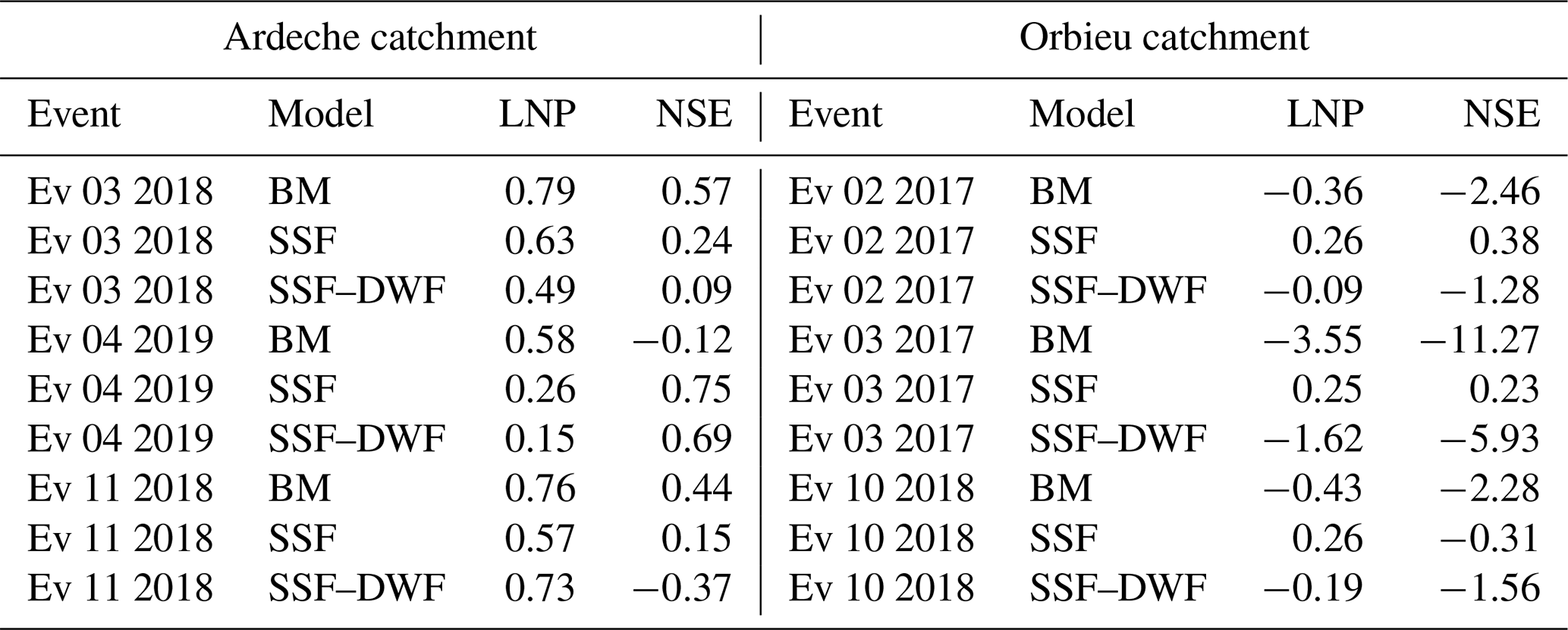
Table 1 The six events considered in this work for the Ardeche catchment in Vogue and the Orbieu catchment in Lagrasse with cumulated volume (Precip.), maximal intensity ($I_{\max }^{\mathrm{pr}}$) of ANTILOPE QPE, and maximal hourly observed discharge ($Q_{\max }^{\mathrm{obs}}$). The stars indicate the return period of the flood: ^* for a 2 year, ${}^{**}$ for a 5 year, and ${}^{***}$ for a 100 year return period. The given dates and duration are those considered for the hydrological simulations. SS is the initial SSD provided by the SAFRAN-ISBA-MODCOU chain for the first day of the simulations, on average, over the catchment.

2.3 Available soil moisture data

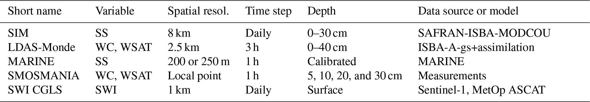
Table 2 summarizes the five products compared in this work for soil moisture estimation: the SAFRAN-ISBA-MODCOU (SIM) root-zone saturation degree, the LDAS-Monde root-zone soil water content, the CGLS Soil Water Index (SWI), and the soil water content measurements provided by the SMOSMANIA network. For the LDAS-Monde and SMOSMANIA data, the SSD is retrieved by dividing the soil water content values by its saturation value in the respective product.

Table 2 Summary of the five products compared in this work for soil moisture estimation. Shown are the SSD (SS), soil water content (WC), soil water content at saturation (WSAT) or Soil Wetness Index (SWI), the spatial and temporal resolution of the product, and the data source or the model used to obtain the product.

2.3.1 The SAFRAN-ISBA-MODCOU products

The SAFRAN-ISBA-MODCOU (SIM) operational modeling chain uses the ISBA surface scheme coupled with the MODCOU hydrological model for underground flows and forced by the SAFRAN atmospheric reanalysis (Habets et al., 2008). SIM outputs have been available since 1958 on an hourly basis, on a regular mesh, and at 8 km resolution. In particular, SIM provides volumetric soil water content for the root layer of the soil. This work uses the outputs of two available versions of SIM: SIM1, which uses the force-restore version of ISBA, ISBA-3L (Noilhan and Planton, 1989; Noilhan and Mahfouf, 1996), and SIM2, which uses the diffusive version of ISBA, ISBA-DIF, with a vertical soil column discretization into a maximum of 14 layers (Decharme et al., 2011). In ISBA-3L, the root zone corresponds to the second soil layer. In ISBA-DIF, the water content of the root zone is considered the sum of the water content of the ISBA-DIF layers between 10 and 30 cm deep for this specific study. The daily soil water content of SIM corresponds to the value at 06:00 UTC each day. The SIM1 and SIM2 chains provide both the volumetric soil water content and soil water content at saturation for the root zone. The SSD of the root zone (i.e., the volumetric soil water content divided by its value at saturation) is directly provided by the SCHAPI for this work. The root-zone SSD provided by the SIM1 product is used for the initialization of the SSD in MARINE, as it is the product used by Douinot et al. (2018) and Garambois (2012) to calibrate the MARINE model. The SIM2 SSD is compared to the SSD simulated with MARINE.

2.3.2 The LDAS-Monde product

LDAS-Monde is a data-assimilation framework that assimilates satellite derived data into the ISBA land surface model (Albergel et al., 2017). It uses the ISBA-A-gs model, which is the CO₂-responsive version of ISBA (Calvet et al., 1998). ISBA-A-gs allows us to simulate photosynthesis and fluxes of CO₂. The diffusive version of ISBA (ISBA-DIF) is used. In addition, LDAS-Monde assimilates LAI (Leaf Area Index) data provided by the European service Copernicus Global Land (CGLS), with a sequential assimilation algorithm (Simplified Extended Kalman Filter). The contribution of the assimilation of satellite data for the simulation of surface fluxes has been tested for various application cases, in particular over Europe and France by Fairbairn et al. (2017), Leroux et al. (2018), Dewaele et al. (2017), and Barbu et al. (2011). In this work, the version of LDAS-Monde that uses the AROME atmospheric model outputs for the atmospheric forcing of the model is used (Albergel et al., 2018; Bonan et al., 2020). These AROME-forced outputs have been available since July 2017 at 2.5 km resolution and at 3 h time steps.

For the two considered catchments, the soil column is discretized into 11 layers with fixed depths. The depth of the total soil column considered for LDAS-Monde is 300 cm for the two catchments. LDAS-Monde provides both the soil water content and maps of soil water content at saturation for each of the 11 layers. For each layer, the SSD is retrieved by dividing its soil water content by the soil water content at saturation. The choice is made in this work to synthesize the 11 LDAS-Monde layers as three average layers: the surface layer (average of layers 1 to 5), deep layer (average of layers 6 to 11), and total layer (average of all 11 layers). Thus, the surface layer represents depths from 0 to 40 cm and the deep layer represents depths from 40 cm to 300 cm. The SSD of the surface layer is noted HU_surf and it is computed as the average of the SSD of layers 1 to 5. The SSD of the deep layer is noted HU_deep and it is computed as the average of the SSD of layers 6 to 11.

2.3.3 The CGLS Soil Water Index product

The Copernicus Global Land Service (CGLS) provides Soil Water Index (SWI) values at 1 km spatial resolution and at the daily time step (Bauer-Marschallinger et al., 2018a). The SWI product combines the Sentinel-1 C-SAR band data and MetOp ASCAT data, in accordance with the algorithm presented by Bauer-Marschallinger et al. (2018b). In this work, the SWI values provided for the top 5 cm of soil are considered. The CGLS SWI product presents good data availability, despite some events being less covered than others (e.g., March 2018 or November 2018 over the Orbieu catchment). In this product, the number of informative pixels per catchment for the studied cases is greater than 14 % of the catchment area. Despite the SWI variable not being directly commensurable with the SSD variable, the CGLS SWI product is taken into account to perform the comparison with the dynamics of the SSD simulated in MARINE. Other products were considered for comparison but they were ultimately not retained as detailed in Appendix A.

2.3.4 The SMOSMANIA network

The SMOSMANIA project (Soil Moisture Observing System Meteorological Automatic Network Integrated Application; Calvet et al., 2007; Parrens et al., 2012) provides soil water content measurements for 21 stations of the automatic ground station network of Météo-France (the RADOME network) along a 400 km Mediterranean–Atlantic transect in southwestern France. Each SMOSMANIA station is equipped with four ThetaProbe ML2X instruments forming a soil profile at depths of 5, 10, 20, and 30 cm. Volumetric soil water content is recorded at each depth and data have been transmitted every 15 minutes from all the stations since 2006. Two stations are considered for this work: the Mouthoumet station in the Orbieu catchment in Lagrasse and the Barnas station in the Ardeche catchment in Vogue. For these two stations, soil moisture profiles are available over the whole 2017–2019 period. The sensor calibrations are regularly checked and the vertical variability of the soil properties is taken into account for these calibrations. For each sensor, the SSD is retrieved by dividing the measured soil water content by its value at saturation estimated at the location of the point of measurement.

3 Methods

3.1 Comparison protocol

The SMOSMANIA observation network provides valuable information for the upper soil water content. However, scale differences exist between the point measurements and the gridded simulated soil water content. Various strategies might be used to resolve this issue, among which is averaging at a large timescale (Tramblay et al., 2010; Fuamba et al., 2019). In this study, considering the fast-evolving processes involved, we choose to maintain the hourly time step for soil moisture analysis. The important spatial variability of the soil moisture is then taken into account by spatial averaging of the gridded simulated values around the measurement point. In order to consider equivalent surfaces for the grids simulated in MARINE and provided by the LDAS-Monde and CGLS data, the MARINE SSD maps are averaged on a 1 km² area around the measurement point. In addition, among the MARINE grid cells, some are part of the river drainage network. As the physics of the SSD in the drainage network are not the same as over hillslope cells, the cells corresponding to the MARINE drainage network are excluded from the 1 km² area around the measurement point. For the Ardeche catchment, four drainage cells are excluded from the 16 cells around the measurement point. For the Orbieu catchment, no drainage cells are located within 1 km² around the measurement point, so no cells are excluded.

Concerning the comparison between the MARINE simulation and LDAS-Monde, for the base and SSF models, which use a one-layer soil discretization, the MARINE SSD is compared to the HU_surf values. For the SSF–DWF model, which uses a two-layer soil discretization, the saturation degree of the MARINE upper layer is compared to LDAS-Monde HU_surf values, and the saturation degree of the MARINE deep layer is compared to the LDAS-Monde HU_deep values. The total average LDAS-Monde layer is used for overall comparison. The behaviors of each of the 11 soil layers in LDAS-Monde are presented in Appendix B.

3.2 Indices

The performance of the simulated discharges is estimated at the hourly time step through the usual Nash and Sutcliffe (1970) criteria (NSE) and also through the LNP index, defined by Roux et al. (2011) as in equation 1, where Q^obs ($Q_{\max }^{\mathrm{obs}}$) and Q^sim ($Q_{\max }^{\mathrm{sim}}$) represent the (maximal) observed and simulated discharged, respectively. Discharges are expressed in m³ s⁻¹. $T_{\max }^{\mathrm{obs}}$ (respectively, $T_{\max }^{\mathrm{sim}}$) is the time (in seconds) when the observed (respectively, simulated) discharge reaches it maximum value. T_{concentration} (in seconds) is the concentration time of the catchment. The advantage of the LNP index is to give equal weight to the NSE values (first term), to the peak value estimation (second term), and to the timing of the peak simulation (third term). LNP appears to be an integrative criteria well suited for flash flood modeling (Lovat et al., 2019).

$$\begin{array}{}\text{(1)}& \begin{array}{rl}\mathrm{LNP}& ={\displaystyle \frac{\mathrm{1}}{\mathrm{3}}}\cdot (\mathrm{1}-{\displaystyle \frac{{\sum }_i(Q_i^{\mathrm{sim}}-Q_i^{\mathrm{obs}}{)}^{\mathrm{2}}}{{\sum }_i(Q_i^{\mathrm{obs}}-\stackrel{\mathrm{‾}}{Q_i^{\mathrm{obs}}}{)}^{\mathrm{2}}}})\\ & +{\displaystyle \frac{\mathrm{1}}{\mathrm{3}}}\cdot (\mathrm{1}-{\displaystyle \frac{\mid Q_{\max }^{\mathrm{sim}}-Q_{\max }^{\mathrm{obs}}\mid }{Q_{\max }^{\mathrm{obs}}}})\\ & +{\displaystyle \frac{\mathrm{1}}{\mathrm{3}}}\cdot (\mathrm{1}-{\displaystyle \frac{\mid T_{\max }^{\mathrm{sim}}-T_{\max }^{\mathrm{obs}}\mid }{T_{\mathrm{concentration}}^{\mathrm{obs}}}})\end{array}\end{array}$$

The comparison of the SSD simulated in MARINE and provided by LDAS-Monde is performed at the catchment scale using the relative bias and Kendall correlation over values averaged at the catchment scale. In addition, the spatial dynamics of the simulated SSD are quantified using the spatial moments δ₁ and δ₂ defined by Zoccatelli et al. (2011). The δ₁ and δ₂ moments take into account the distance of each grid cell to the drainage network and they allow us to represent both the overall location of the SSD field with respect to the outlet and the number of modes (i.e., concentration points in this case) of the field. The exact formulation of the δ₁ and δ₂ spatial moments as functions of the spatially distributed field and of the distance to the river network can be found in Eqs. (2) and (3) in Zoccatelli et al. (2011). The closer the δ₁ values are to 1, the more centered around the centroid of the catchment is the field. Values of δ₁ lower than 1 mean that the field gets closer to the outlet. Values of δ₁ higher than 1 characterize a field globally located on the upstream part of the catchment. The closer the δ₂ values are to 1, the more uniform is the distribution of the field. Values of δ₂ lower than 1 represent a unimodal distribution of the field. Values of δ₂ higher than 1 represent a multimodal distribution. Despite being initially defined by Zoccatelli et al. (2011) to characterize rainfall fields, the δ₁ and δ₂ moments also appear to be particularly relevant when applied to the SSD fields.

3.3 Model setup

3.3.1 Parametrization and precipitation forcing

The MARINE model requires the definition of (i) the digital elevation model (DEM), (ii) soil survey data to compute the hydraulic and storage properties of the soil, and (iii) land-use data to configure the surface roughness parameters. The IGN-25 m DEM is used in this work. The soil depths and soil texture maps are taken from the INRA soil database for the Ardeche and Languedoc-Roussillon regions (Robbez-Masson et al., 2000). The parameters of the pedotransfer function are computed based on the USDA soil classification (Spaargaren and Batjes, 1995). Land cover is provided by the Corine Land Cover 2006 database (Aune-Lundberg and Strand, 2010). This study uses the calibration of MARINE provided by Garambois et al. (2015b) for the Orbieu catchment and by Douinot et al. (2018) for the Ardeche catchment. The base model has been thoroughly tested over the last 10 years or so, including in the catchments studied in this work (Roux et al., 2011; Garambois, 2012; Garambois et al., 2015a; Douinot et al., 2018), whereas the SSF–DWF model has just been developed. The model is set up over a regular mesh. The spatial resolutions applied by Garambois et al. (2015b) and Douinot et al. (2018) for the calibration are kept. For the Orbieu catchment, the spatial resolution is 200 and 250 m for the Ardeche catchment.The ANTILOPE QPE data are used as hourly precipitation input for the MARINE model, available at the kilometric resolution. Despite the precipitation information being given at an hourly time step, the sub-hourly processes are simulated using a 5 min computation time step and results are aggregated at an hourly time step. Figure 3 presents the IGN-25 m DEM and the soil depth maps used for the two studied catchments. Table 3 presents the calibrated parameter values obtained for each catchment by Douinot et al. (2018) and Garambois et al. (2015b) and used in this work.

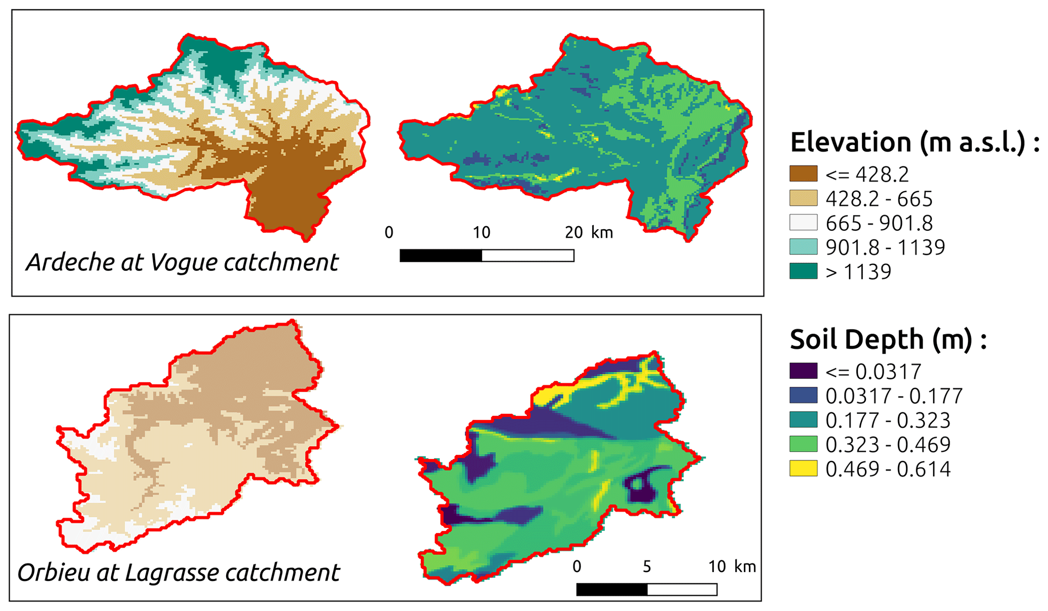
Figure 3 The IGN-25 m DEM and soil depth maps from the INRA soil database used for MARINE parametrization for the two studied catchments.

Douinot et al. (2018)Garambois et al. (2015b)

Table 3 Calibrations obtained by Douinot et al. (2018) and Garambois et al. (2015b) for the Orbieu catchment in Lagrasse and the Ardeche catchment in Vogue. Shown are the multiplier coefficient for soil depth maps (C_z), the multiplier coefficient for the spatialized saturated hydraulic conductivity used in lateral flow modeling (C_kss), the multiplier coefficient for the spatialized hydraulic conductivity at saturation that is used in infiltration modeling (C_kga), two friction coefficients for low- and high-water channels (C_D1 and C_D2), and the deep layer depth for the SSF–DWF model ($C_z^{\mathrm{deep}}$).

3.3.2 Discharge simulation

Figure 4 presents the discharges at the outlets simulated with MARINE using the base, SSF, or SSF–DWF models together with the observed discharges during the flood events. Table 4 presents the associated LNP and Nash–Sutcliffe efficiency (NSE) performance criteria of the simulated discharges, referring to hourly observed discharges. The main effect of computing the transfers through the subsurface as a function of the volumetric soil water content instead of the water height (SSF model) is to flatten the overestimation of the simulated discharge during the flow rise at the beginning of the events. This behavior will be explained in the Results section; there is no gradient of initial soil water content over the 8 km × 8 km SIM mesh. Therefore, the contribution of the subsurface to the discharge at the beginning of the events is smaller in the SSF and SSF–DWF than in the base model. However, in the SSF–DWF model, these dynamics are influenced by the contribution of the deep layer, which is controlled by the parametrization of the thickness of this deep layer. Nevertheless, the calibrations of the three models clearly require improvement in order to better simulate the discharges at the outlets, in particular for the Orbieu catchment and for the SSF–DWF model. However, since this paper focuses on comparing the SSD dynamics simulation according to the soil physics considered in the model and considering that the variety in the structures of the considered events (see Sect. 2.2.2) limits model accuracy, the calibrations proposed by Douinot et al. (2018) and Garambois et al. (2015b) are directly applied to this work. As the SSF model does not involve additional parameters, the same calibration is used for the SSF and base models, as given by Douinot et al. (2018) for the Ardeche catchment and Garambois et al. (2015b) for the Orbieu catchment. The SSF–DWF model also involves calibrating the depth of the deep layer. Therefore, the calibrations of the SSF–DWF model performed by Douinot et al. (2018) for both the Orbieu and the Ardeche catchments are used.

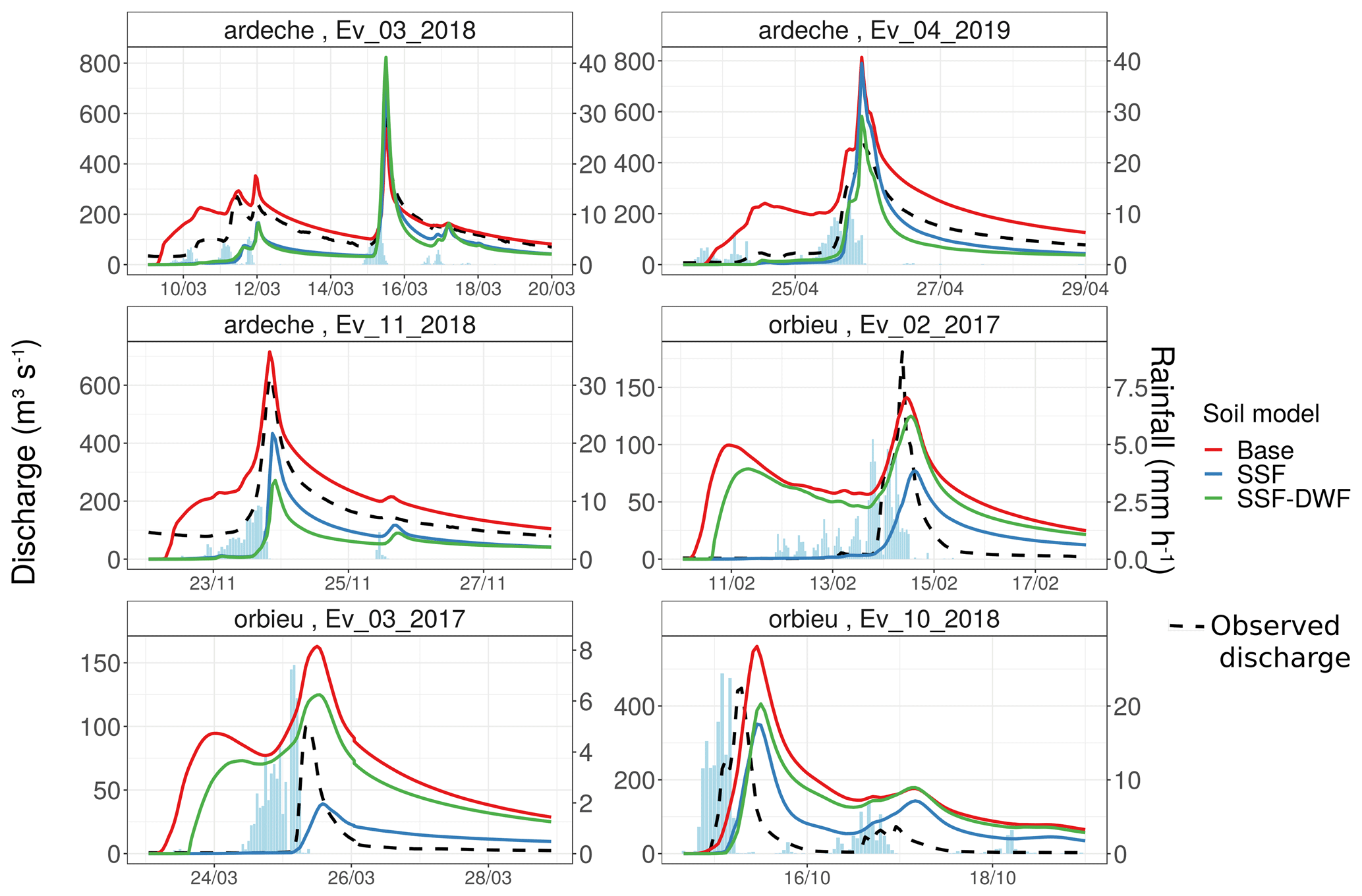
Figure 4 Discharges at the outlets of the Ardeche and Orbieu catchments for the six studied events simulated with MARINE using the base, SSF, and SSF–DWF models, and the observed discharges.

Table 4 LNP and Nash–Sutcliffe efficiency (NSE) performance criteria for discharge simulation at the outlet for the six studied events over the two catchments for the base model (BM), the subsurface flow model (SSF), and the subsurface flow model coupled with the deep water model (SSF–DWF), referring to hourly observed discharges.

4 Results and discussions

4.1 Comparison at the point measurement scale

Figure 5 combines (i) the SSD measurements at the four sensor depths for the Barnas (for the Ardeche catchment) and the Mouthoumet (for the Orbieu catchment) SMOSMANIA stations; (ii) the SSD simulated with MARINE, on average, over a 1 km² area over the station location (see Sect. 3.1; for the simulations using the SSF–DWF soil model, the moisture of the surface layer is considered here); (iii) the LDAS-Monde surface SSD HU_surf for the 2.5 km × 2.5 km grid cell that contains the SMOSMANIA station; and (iv) the CGLS SWI when available for the 1 km × 1 km grid cell that contains the SMOSMANIA station for the Orbieu catchment. No CGLS SWI data are available for the grid cell that contains the station for the Ardeche catchment. Table 5 provides the Kendall correlations associated with the hourly time series presented in Fig. 5. The values in bold are the best correlation values between the SMOSMANIA measurements and the MARINE outputs or the LDAS-MONDE HU_surf for each event.

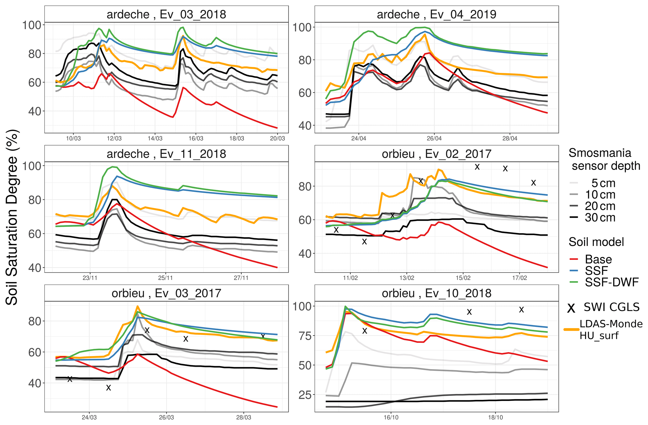
Figure 5 SMOSMANIA SSD measurements at the four sensor depths for the Barnas (Ardeche catchment) and the Mouthoumet (Orbieu catchment) stations, together with the SSD simulated with MARINE, the LDAS-Monde HU_surf, and the CGLS SWI when available at the measurement point location. For the MARINE simulations using the SSF–DWF soil model, the moisture of the surface layer is considered here.

The dynamics of soil saturation degree simulated with the base model differ significantly from the simulations using the SSF and SSF–DWF models. The soil layer empties faster with the base model, leading to a simulated SSD significantly lower than the SSF and SSF–DWF models. For the simulated events overall, the simulated SSD and the SMOSMANIA measurements appear to be better correlated when using the SSF–DWF model than the base model or SSF model. The soil physics used in the SSF–DWF model, i.e., the use of the volumetric soil water content rate and the vertical discretization into two layers, allows us to enhance the SSD simulation for the surface layer with respect to in situ measurements. This point will be developed by considering the catchment average of simulated SSD in the next section.

In addition, the SSD output of the SSF–DWF model are generally larger than the output of the base and SSF models. This behavior can be explained by the fact that for the SSF–DWF model, the depths of the upper layer are taken from the INRA soil database, whereas for the base and SSF models, a multiplicative, calibrated coefficient greater than 1 is applied. Consequently, the depths considered for the surface layer are thinner in the SSF–DWF than in the base and SSF models. The saturation of the surface layer is then reached faster.

In addition, the LDAS-Monde HU_surf appears to be globally satisfyingly correlated with the SMOSMANIA measurements, with slightly different correlations for the four sensor depths. This shows that the dynamics of the LDAS-Monde HU_surf variable is locally significant with in situ surface SSD measurements. The reliability of the LDAS-Monde HU_surf dynamics for the surface SSD description can thus be considered satisfying. On the contrary, the correlation between the daily CGLS SWI values and both the MARINE outputs and the SMOSMANIA measurements appear to be low. However, a more extensive study of the validity of this product at the local scale would be needed to draw further conclusions.

Table 5 Kendall correlations between SMOSMANIA measurements at each depth and the MARINE SSD simulated with each soil model or the LDAS-Monde HU_surf . The values in bold are the best correlations between the SMOSMANIA measurements and the MARINE outputs or the LDAS-MONDE HU_surf for each event.

4.2 Comparison at the catchment scale

4.2.1 Catchment average behavior

Figure 6 presents the soil saturation degree time series, on average per catchment, simulated with MARINE using the base, SSF, or SSF–DWF models, together with the catchment average of the LDAS-Monde HU_surf, the daily CGLS SWI values, and the daily SIM2 HU values (see Sect. 2.3.1). When the SSF–DWF model is applied, the surface layer is considered here. Table 6 presents the Kendall correlations associated with the hourly times series. The same observations as for the comparison at the local scale can be drawn: both the dynamics and amplitudes of the SSD simulated with the base model significantly differ from the outputs of the two other models. When no precipitation happens, the soil drainage in the base model is faster than for the SSF and SSF–DWF models. In addition, the SSD simulated with the SSF–DWF model is globally higher than the one simulated with the SSF model, on average per catchment. The SSD simulated with the SSF–DWF model appears to be better correlated with the LDAS-Monde HU_surf time series for four of the six studied events. Considering that the dynamics of the LDAS-Monde HU_surf are of satisfying accuracy (see Sect. 4.1), the SSF–DWF model appears to improve the simulation of the dynamics of the surface layer moisture compared to both the SSF and base models. This result appears to be particularly reliable, since it is observed both at the point measurement scale and at the catchment scale. It can be physically explained by the fact that in the SSF and SSF–DWF models, the lateral transfers are computed as a function of the volumetric soil water gradients, whereas in the base model, they are computed as a function of the water height gradient. Indeed, since the water height gradient between two cells depends on the slope between the cells and the cell textures, water height gradients are larger than volumetric soil water gradients when no precipitation happens. Consequently, lateral flows based on the water height gradients are larger than lateral flows based on the volumetric soil water gradients.

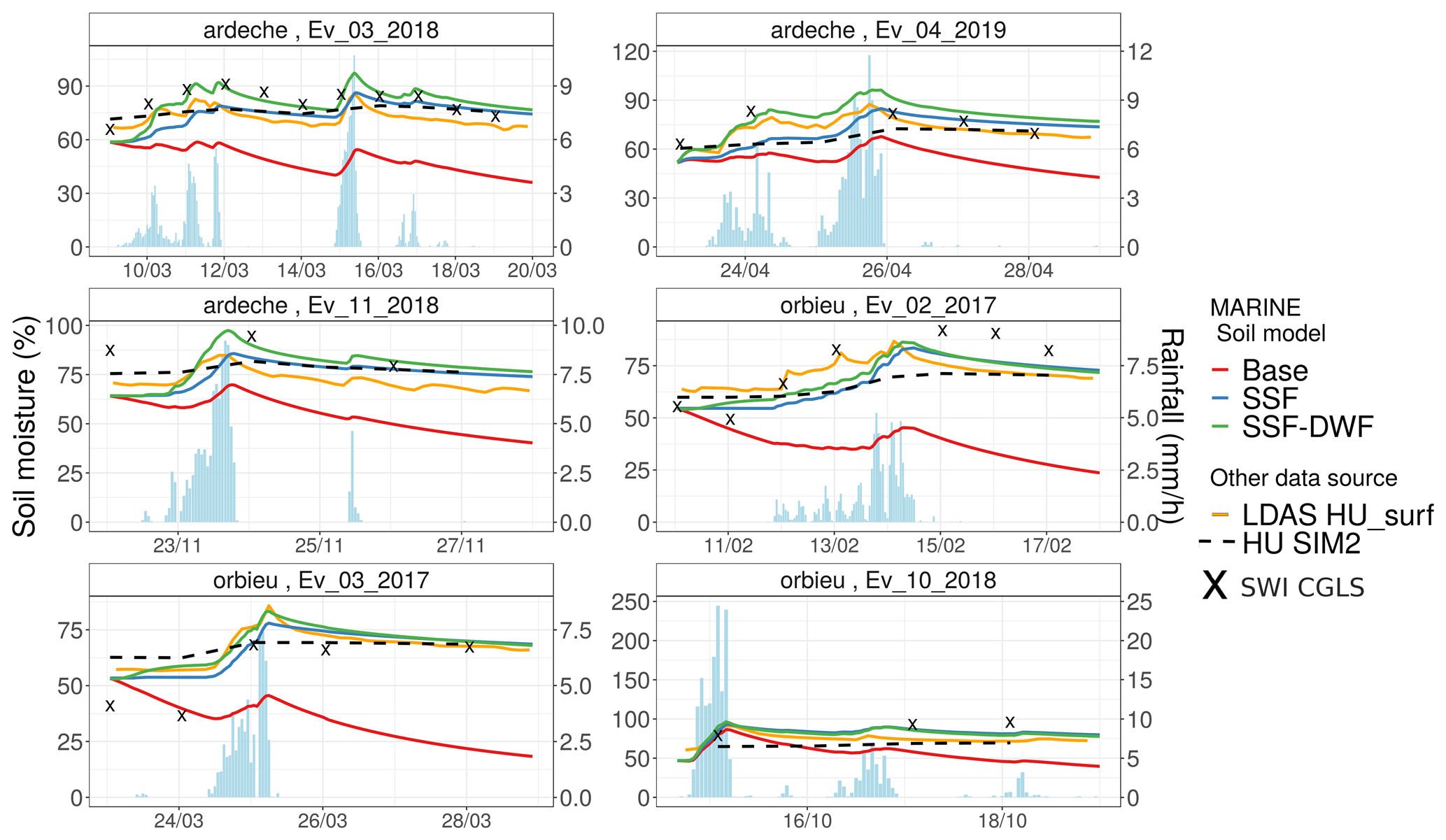
Figure 6 Catchment average of the SSD time series simulated with MARINE using the base, SSF, or SSF–DWF models, together with the catchment averages of the LDAS-Monde HU_surf and SWI CGLS values for the two studied catchments and the six studied events.

Overall, the temporal dynamics of the CGLS SWI, on average per catchment, are more consistent with the SSF and SSF–DWF model outputs than with the base model output. In particular, for the events of February and March 2017 in the Orbieu catchment, the sharp decrease of the SSD simulated in the base model is not observed in the CGLS SWI values. In addition, for the March 2018 event in the Ardeche catchment, which is the longest of the studied events, the dynamics of the CGLS SWI are consistent with the SSD simulated with the SSF and SSF–DWF models. Likewise, catchment averages of the SIM2 HU values are also better correlated with the SSF and SSF–DWF model outputs than with the base model output, despite the range of variation of the daily SIM2 HU values being narrower than the range for the CGLS SWI values.

4.2.2 Spatial variability

Figure 7 presents maps of the SSD simulated with the base, SSF, and SSF–DWF models, and the maps of LDAS-Monde HU_surf for the example of the November 2018 event in the Ardeche catchment. The daily products are not presented here because the daily time step does not allow us to represent the fast-evolving flood processes. Four time steps of the simulation are considered: the first time step of the run, one time step during the flow rise, the peak flow hour, and one time step during the flow decrease. This example illustrates the results previously described: the saturation of the surface layer is reached faster for the SSF–DWF model than in the others. In addition, the spatial pattern of the SSD simulated with MARINE appears to be consistent with LDAS-Monde HU_surf maps. These results are also observed for the other events, which are not presented here.

Figures 8 and 9 present the δ₁ and δ₂ spatial moments computed for the MARINE SSD outputs, the LDAS-Monde HU_surf, and the CGLS SWI at the daily time step. Since no lateral transfers are represented in the LDAS-Monde and the CGLS SWI products, the MARINE drainage network is used to compute the spatial moments for both of them. The distinction between the base model outputs and the SSF and SSF–DWF model outputs can still be made. The general behavior of the δ₁ spatial moment when computed on the SSD is that the δ₁ increases when precipitation happens and then decreases at a variable rate. Indeed, as precipitation necessarily flows towards the outlet, δ₁ values are bound to increase (i.e., the SSD fields get closer to the outlet after a precipitation event.) The δ₁ time series obtained with both the SSF and SSF–DWF models are significantly closer to 1 than the δ₁ values obtained with the base model. This means that the SSD fields simulated with the base model are globally closer from the outlet than with the SSF and SSF–DWF models, that is to say that the propagation of the water through the drainage network in the upper soil layer is faster for the base model than for the SSF and SSF–DWF models. The analysis of the δ₁ time series allows us to quantify the impact of the calibration of lateral transfers on the SSD distribution.

The general behavior of the δ₂ spatial moment is that the δ₂ decreases with precipitation, with SSD fields more centered around the area of maximum rainfall, and then increases with the spread of the SSD fields along the drainage network. The δ₂ values for the SSF and SSF–DWF models are globally closer to 1 than for the base model; that is to say that the SSD fields simulated with the SSF and SSF–DWF models are globally more uniform than with the base model. This can be explained by the fact that the SSD is globally higher for the SSF and SSF–DWF models than for the base model (see Fig. 6), the difference between the SSD and saturation in the drainage network (i.e., 100 %) is stronger for the base model than for the other two models. This leads to SSD fields being more uniform for the SSF and SSF–DWF models than for the base model. This result is particularly observed for the Orbieu catchment. The analysis of the δ₂ time series allows us to quantify the differences between the base model on the one side and the SSF and SSF–DWF models on the other side.

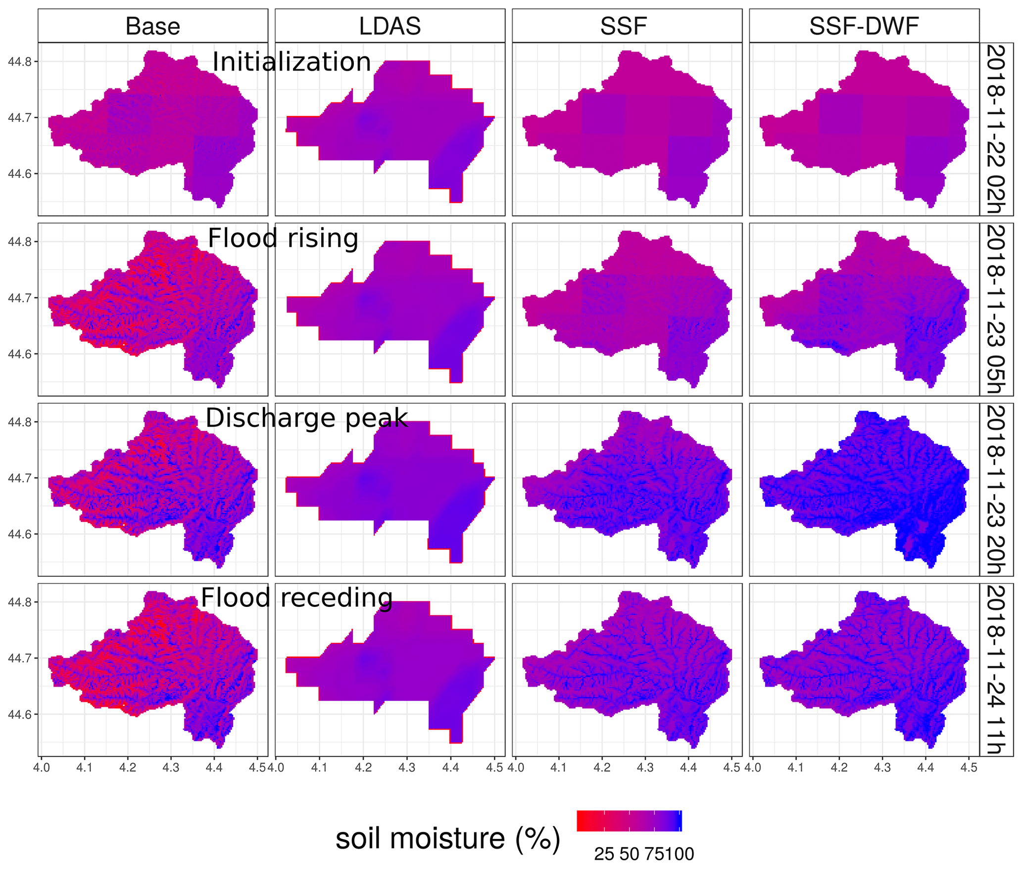
Figure 7 Maps of simulated SSD for the example of the November 2018 event in the Ardeche catchment. MARINE simulation output with the base, SSF, and SSF–DWF models are presented as well as the LDAS-Monde HU_surf maps. Four time steps of the simulation are considered: the first time step of the run, one time step during the flow rise, the peak flow hour, and one time step during the flow decrease.

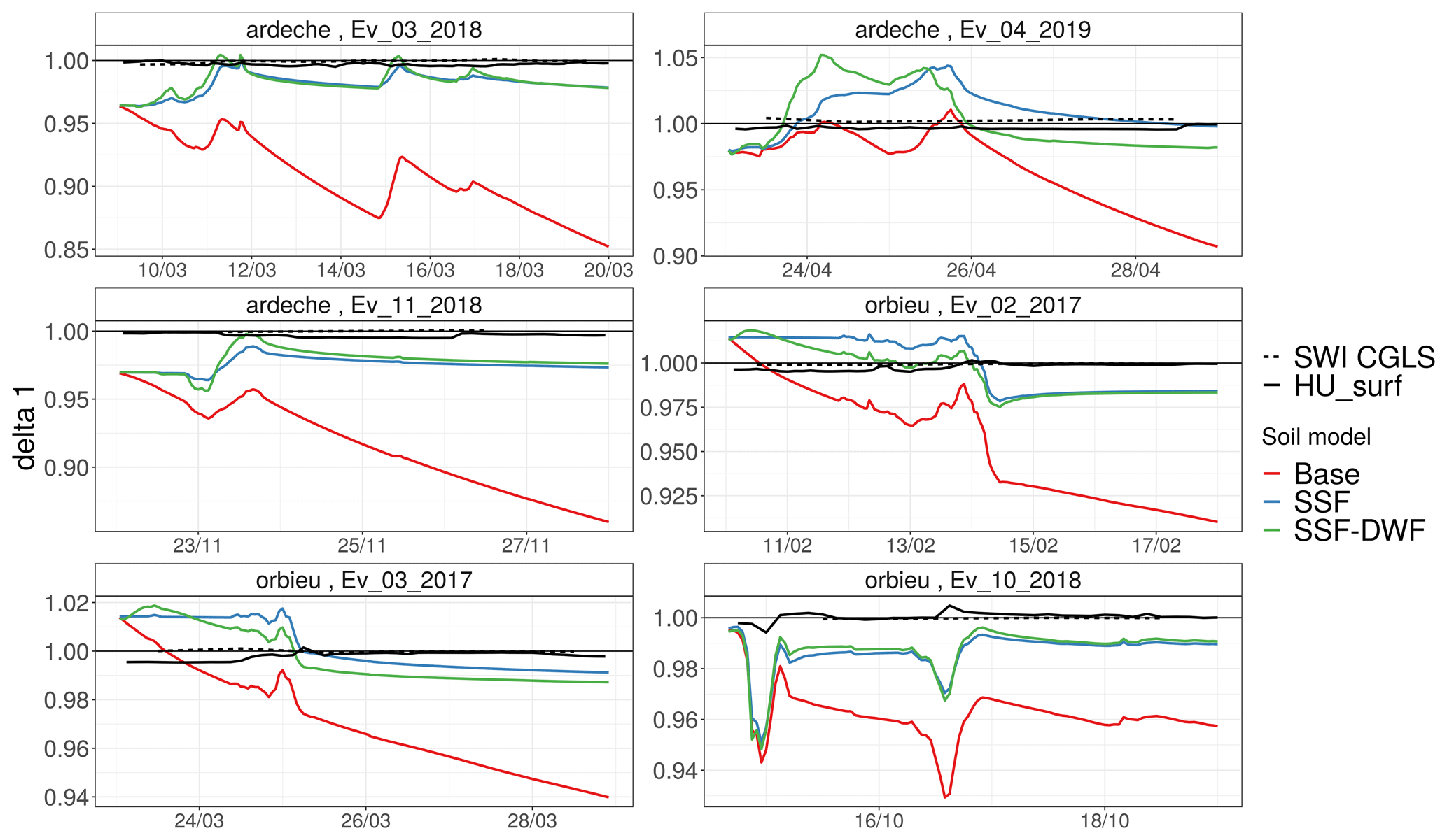
Figure 8 Time series of index δ₁ defined by Zoccatelli et al. (2011) for the six events, computed for the SSD outputs for the BM, SSF, and SSF–DWF models, and also for the LDAS-Monde HU_surf variable and the CGLS SWI.

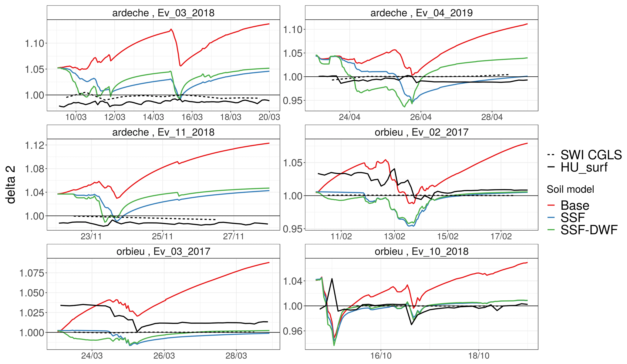
Figure 9 Time series of index δ₂ defined by Zoccatelli et al. (2011) for the six events, computed for the SSD outputs for the BM, SSF, and SSF–DWF models, and also for the LDAS-Monde HU_surf variable and the CGLS SWI.

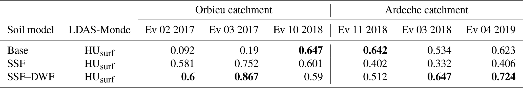
Table 6 Kendall correlations between LDAS-Monde HU_surf and MARINE SSD, on average per catchment, for each soil model. The values in bold are the best correlations between the MARINE outputs and the LDAS-MONDE HU_surf for each event.

Both the δ₁ and δ₂ spatial moments computed for the LDAS-Monde HU_surf are globally closer to 1 than when computed for the MARINE outputs. Indeed, since the spatial resolution of the LDAS-Monde HU_surf product is 2.5 × 2.5 km², whereas it is 200 × 200 or 250 × 250 m for the MARINE simulations, the spatial variability of the LDAS-Monde HU_surf is lower than for the MARINE outputs. The δ₁ and δ₂ spatial moments computed for the CGLS SWI are very close to 1, with tiny variations. This can be explained by the facts that (i) the spatial resolution of the CGLS SWI grids is coarser than the MARINE resolution and (ii) the number of missing pixels is important in the CGLS SWI product, in particular for the Ardeche catchment.

The analysis of the δ₁ and δ₂ spatial moments provides an innovative way to assess the spatial variability of the SSD fields. The reaction of the SSD fields to precipitation are quantified. The difference between the spatial repartition of the outputs of the base model on the one side and the SSF and SSF–DWF models on the other side is highlighted.

Table 7 Kendall correlations between the LDAS-Monde HU_deep and deep layer moisture simulated with MARINE using the SSF–DWF model.

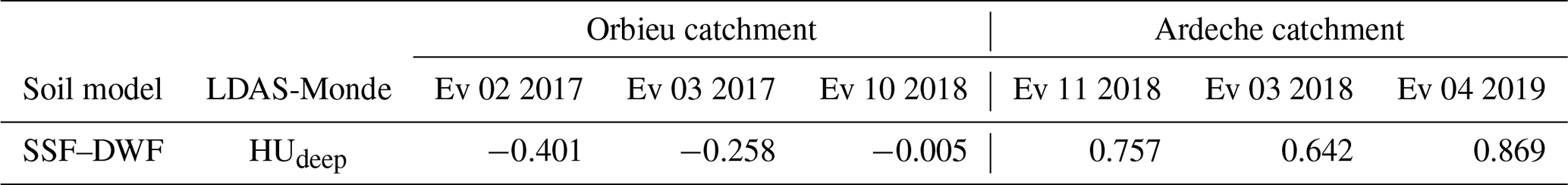
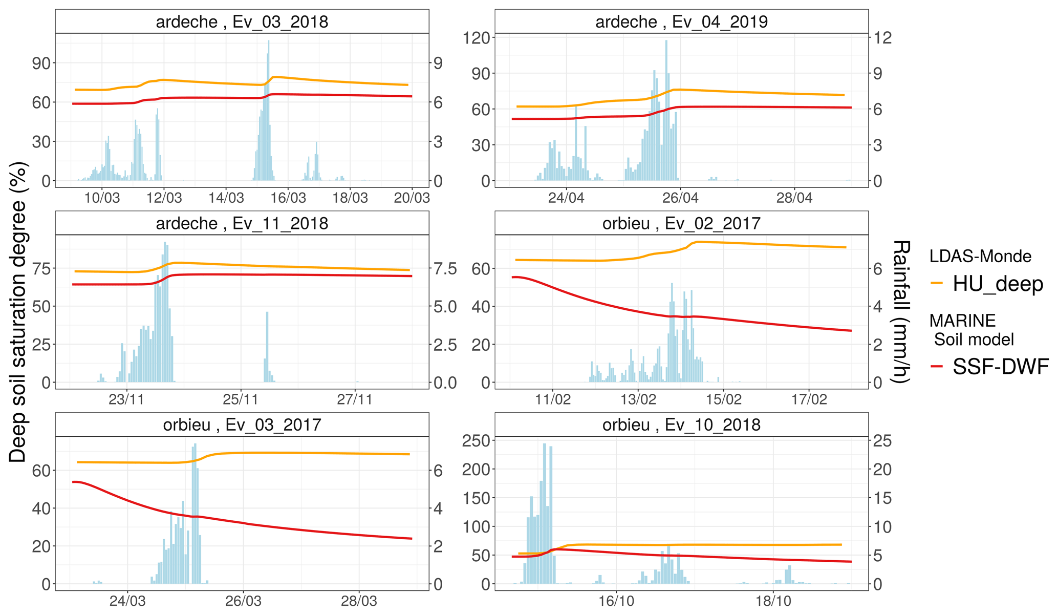
Figure 10 The SSD simulated for the deep layer with the SSF–DWF model, together with the LDAS-Monde HU_deep time series, on average per catchment.

4.2.3 Water content of the deep layer

Figure 10 presents the SSD simulated for the deep layer with the SSF–DWF model, together with the LDAS-Monde HU_deep time series, on average per catchment. Table 7 presents the Kendall correlations between the SSF–DWF deep layer moisture and the LDAS-Monde HU_deep.

For the Ardeche catchment, the simulated deep layer moisture is well correlated with the LDAS-Monde HU_deep, with Kendall correlations between 6.4 % and 8.7 %. This result enhances the reliability of the deep layer calibration in the SSF–DWF model for the Ardeche catchment. For the Orbieu catchment, the simulated deep layer moisture appears not to be consistent with the LDAS-Monde HU_deep, in particular for the two events of February and March 2017. For the strong October 2018 event in the Orbieu catchment, the sharp increase of the deep SSD at the end of the rainfall event is observed in both the SSF–DWF model and in the LDAS-Monde HU_deep. For the Ardeche catchment, the good correlations between the LDAS-Monde HU_deep and the deep layer moisture simulated with the SSF–DWF model highlights the consistency of this model for this catchment and it corroborates the results of Douinot et al. (2018), which tend to show that this model is particularly suitable for discharge simulation in shale watershed. Conversely, for the Orbieu catchment, the weak correlations between the LDAS-Monde HU_deep and the SSF–DWF model output corroborates the fact that this model seems less suited for sedimentary catchments. These results illustrate the difficulty in representing the hydrological dynamics of the deep soil layers, the limitation being the lack of knowledge concerning the physical description of the subsurface water storage (Martin et al., 2004; Maréchal et al., 2013; Vannier et al., 2016).

The calibration of the deep layer in the SSF–DWF model for the Orbieu catchment leads to an emptying of the deep SSD faster than for the LDAS-Monde HU_deep variable. The simulation of the deep layer water content strongly depends on the calibration of the deep layer thickness, the deep layer porosity, and the vertical and lateral hydraulic conductivities in the deep layer. In this work, the vertical and lateral hydraulic conductivities of the deep layer are considered to be equal. Additional research regarding the deep layer calibration is needed. In particular, the Height Above Nearest Drainage (HAND) method would offer the opportunity to take into account the terrain physical characteristics in the deep layer parametrization (Nobre et al., 2011).

5 Conclusions

The local comparison of the MARINE outputs for surface soil saturation with the SMOSMANIA measurements, as well as the comparison at the basin scale with the gridded LDAS-Monde and CGLS data, leads to the same conclusion: the SSD simulated with the base model significantly differs from the simulations using the SSF and SSF–DWF models. When no precipitation happens, the soil layer empties faster with the base model, leading to a simulated SSD significantly lower with the base model than with the two other models. This behavior can be physically explained by the fact that in the SSF and SSF–DWF models, the lateral transfers are computed as a function of the volumetric soil water gradients, whereas in the base model they are computed as a function of the water height gradient. Indeed, since the water height gradient between two cells depends on the slope between the cells and the cell textures, water height gradients are larger than volumetric soil water gradients when no precipitation happens. Consequently, lateral flows based on the water height gradients are larger than lateral flows based on the volumetric soil water gradients. In addition, the dynamics as well as the amplitudes of the SSD simulated in the SSF model and for the upper layer in the SSF–DWF model are better correlated with both the SMOSMANIA measurements and the LDAS-Monde data than the outputs of the base model. Considering that the dynamics of the LDAS-Monde HU_surf are of satisfying accuracy, this assessment leads to the conclusion that the SSF–DWF model improves the simulation of the dynamics of the surface layer moisture, compared to both the SSF and base models. This result appears to be particularly reliable, since it is observed both at the point measurement scale and at the catchment scale.

In the SSF–DWF model, the simulation of the moisture in the deep layer is also compared to LDAS-Monde moisture data provided for deeper layers. However, the simulation of the deep layer water content strongly depends on the calibration of the deep layer thickness, the deep layer porosity, and the vertical and lateral hydraulic conductivities in the deep layer. These results illustrate the difficulty in representing the hydrological dynamics of the deep soil layers, the limitation being the lack of knowledge concerning the physical description of the subsurface water storage. Further conclusions concerning the simulation of the deep SSD would then require extensive work to enhance the parametrization of the deep layer in the SSF–DWF model. In addition, the model performance in terms of flash flood prediction remains weak for the studied events. Additional work on model calibration would thus be needed to enhance the model performance for flash flood prediction.

In conclusion, this work exposes that computing the infiltration flow as a function of the soil saturation degree instead of the water height in the MARINE model enhances the soil moisture simulation during flash floods with respect to both local measurements and spatially distributed products.

Appendix A: Literature review of available satellite derived products

Various products derived from remote imagery are available for soil moisture estimation at various spatial and temporal scales. In particular, the relevance of five products is investigated for this study. Table A1 summarizes the investigated products and their main characteristics.

1. The Copernicus Global Land Service (CGLS) provides both Surface Soil Moisture (SSM) and Soil Water Index (SWI) values at the 1 km spatial resolution and at the daily time step (Bauer-Marschallinger et al., 2018a). The SWI product combines the Sentinel-1 C-SAR band data and the MetOp ASCAT data in accordance with the algorithm presented by Bauer-Marschallinger et al. (2018b), whereas the SSM product is derived from only the Sentinel-1 C-SAR band data. In this work, the SWI values provided for the top 5 cm of soil are considered. The uncertainties for the CGLS SSM are computed by adding the different sources of uncertainty occurring in the product preparation and they represent about 8 % of the SSM values. No uncertainties estimation is provided for the SWI product.

2. The soil moistures with the very high spatial resolution product (VHSR), provided by the THEIA-Land pole (https://www.theia-land.fr, last access: 15 March 2021), offer soil moisture maps with a 6 d frequency and at the sub-parcel scale on several sites in France, in Europe, and around the Mediterranean basin (El Hajj et al., 2017). The THEIA-Land VHSR soil moisture product exploits the Sentinel-1 radar and Sentinel-2 optical Copernicus image series, following a neural network signal inversion algorithm. The extent of the two studied basins is covered by this product. However, since the footprints of the images are variable depending on the dates, the entire catchments are not covered for all dates. The number of gaps in this product is significant; only 12 images are available over the studied events. In particular, no data are available over the Ardeche catchment for the studied dates.

3. The SMOS-IC product provides daily SSM at 25 km resolution (Fernandez-Moran et al., 2017). The SMOS-IC soil moistures are derived from the SMOS satellite data, based on the algorithm presented by Wigneron et al. (2007). This method uses the new calibrated values of the soil roughness and effective scattering albedo parameters presented by Li et al. (2020). The uncertainties associated with the SMOS-IC product are estimated through the TB-RMSE index, presented by Al-Yaari et al. (2019) and represent about 5 % of the SMOS-IC SSM values.

4. The ESA CCI (European Spatial Agency, Climate Change Initiative) product provides surface soil moisture datasets at daily temporal time step and 25 km spatial resolution. In this product, the AMI-WS and MetOp ASCAT C-band data are merged with several radiometer soil moisture products along the algorithm presented by Wagner et al. (2012). The uncertainties associated with the ESA CCI SSM product are considered the variance of the dataset, estimated through triple collocation analysis. Uncertainties represent about 3% of the ESA CCI SSM values.

Figure A1 jointly displays the catchment average for these products over the studied events. The impact of the spatial resolution on the spatially averaged values can be clearly noticed. The coarse resolution (e.g., 25 and 30 km resolution) SMOS-IC and ESA CCI soil moisture products appear to be overly low compared to the products at the kilometric resolution (CGLS and THEIA-Land VHSR). In addition, the ESA CCI product is known to provide globally wetter SSM than the SMOS-IC product, as mentioned by Dong et al. (2020). However, it is to be noted that this product comparison is mainly informative regarding the temporal dynamics of the products, but their respective biases cannot be directly compared, mainly for two reasons: (i) the compared variables are not necessarily commensurable (i.e., SSM and SWI) and (ii) the soil depth considered in each product for the SSM estimation might differ.

Important discrepancies are observed in the temporal dynamics for the different products. Since the study area is rather small, no validation of these products at the catchment scale is available and the relatively low uncertainty estimates provided by the reference publications do not allow us to explain these differences. As no particular temporal behavior can be distinguished among the five products, the choice has been made for this work to particularly focus on the product presenting the best data availability and the finest spatial resolution. For the SMOS-IC and the THEIA-Land VHSR products, and also for the CGLS SSM products, too many values are missing for these data sources to be reliably used. On the contrary, the CGLS SWI product presents good data availability, despite some events being less covered than others (e.g., March 2018 or November 2018 over the Orbieu catchment). In this product, the number of informative pixels per catchment for the studied cases is greater than 14 % of the catchment area. Consequently, in this work, the CGLS SWI product is taken into account to perform the comparison with the soil moisture simulated in MARINE. Nevertheless, this literature exploration of the data available for soil moisture description illustrates the difficulty estimating surface soil moisture based on satellite data at small catchment scales (∼100 km²).

Bauer-Marschallinger et al. (2018b)Bauer-Marschallinger et al. (2018a)El Hajj et al. (2017)Fernandez-Moran et al. (2017)Dorigo et al. (2015, 2017)

Table A1 Investigated satellite derived soil moisture products and their main characteristics. Shown are the data producer, Soil Water Index (SWI) or superficial soil moisture (SSM), spatial resolution, and the satellite imagery used.

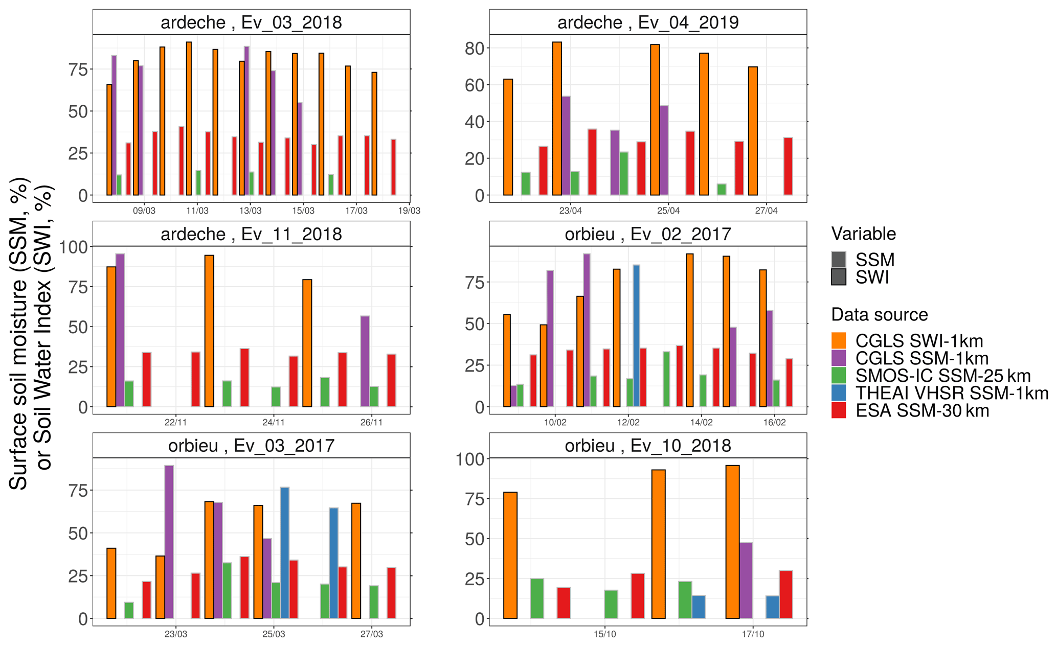
Figure A1 Daily values of Surface Soil Moisture (SSM) or Soil Water Index (SWI) provided by the CGLS, SMOS-IC, THEIA-Land VHSR, and ESA CCI products, on average, over the two studied catchments during the six simulated events.

Appendix B: Choice of layers for the LDAS-Monde soil moisture

Figure B1 presents the spatial average of the soil moisture for each catchment and for each of the 11 soil layers described in the LDAS-Monde product. Two behaviors can be distinguished for the different layers: for the five superficial layers, the response of the soil moisture to precipitation is fast, with important amplitudes; for the deeper layer, the response to precipitation is slower and the amplitude ranges are narrower. Moreover, the diurnal cycle of solar radiation significantly influences up to the fifth layer, i.e., up to 40 cm deep. In addition, over the two studied catchments, the spatial patterns of soil moisture are similar for the 11 layers. Indeed, the spatial distribution of soil moisture is mainly controlled by the soil texture, which is considered as vertically uniform in the ISBA-A-gs model.

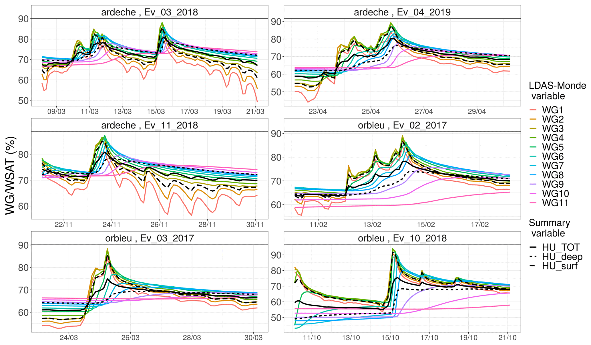
Figure B1 Soil saturation degree (%) for the 11 soil layers described in LDAS-Monde and summary variables HU_surf (average of layers 1 to 5), HU_deep (average of layers 6 to 11), and HU_tot (average of layers 1 to 11), on average per catchment, for the six studied events.