the Creative Commons Attribution 4.0 License.
the Creative Commons Attribution 4.0 License.
 | 05 Mar 2021
Snow water equivalents exclusively from snow depths and their temporal changes: the Δsnow model
Michael Winkler
Harald Schellander
Stefanie Gruber
Reliable historical manual measurements of snow depths are available for many years, sometimes decades, across the globe, and increasingly snow depth data are also available from automatic stations and remote sensing platforms. In contrast, records of snow water equivalent (SWE) are sparse, which is significant as SWE is commonly the most important snowpack feature for hydrology, climatology, agriculture, natural hazards, and other fields.
Existing methods of modeling SWE either rely on detailed meteorological forcing being available or are not intended to simulate individual SWE values, such as seasonal “peak SWE”. Here we present a new semiempirical multilayer model, Δsnow, for simulating SWE and bulk snow density solely from a regular time series of snow depths. The model, which is freely available as an R package, treats snow compaction following the rules of Newtonian viscosity, considers errors in measured snow depth, and treats overburden loads due to new snow as additional unsteady compaction; if snow is melted, the water mass is stepwise distributed from top to bottom in the snowpack. Seven model parameters are subject to calibration.
Snow observations of 67 winters from 14 stations, well-distributed over different altitudes and climatic regions of the Alps, are used to find an optimal parameter setting. Data from another 71 independent winters from 15 stations are used for validation. Results are very promising: median bias and root mean square error for SWE are only −3.0 and 30.8 kg m−2, and +0.3 and 36.3 kg m−2 for peak SWE, respectively. This is a major advance compared to snow models relying on empirical regressions, and even sophisticated thermodynamic snow models do not necessarily perform better. As such, the new model offers a means to derive robust SWE estimates from historical snow depth data and, with some modification, to generate distributed SWE from remotely sensed estimates of spatial snow depth distribution.
- Article
(3672 KB) - Full-text XML
- BibTeX
- EndNote


Depth (HS) and bulk density (ρb) are fundamental characteristics of a seasonal snowpack (e.g., Goodison et al., 1981; Fierz et al., 2009). Their product yields the areal density [kg m−2] of the snowpack, which is often referred to as snow water equivalent (SWE). Water resource management, agricultural applications, hydrological modeling, climate analyses, natural hazard assessments, and many other fields depend on good estimates of SWE. The mass of water stored in the snowpacks is often more relevant than snow depth. Particularly seasonal SWE maxima, i.e., peak SWE (SWEpk), is required for, for example, discharge or flood forecasting as well as analyses of climate and extremes. The latter, in turn, rely on long-term or “historical” data. While measurements of HS are relatively widely available, the more useful value of SWE is more difficult to determine and is consequently relatively poorly known, hampering efforts to understand SWE variance and related vast management practices. To address this limitation, this paper focuses on developing a robust method to derive SWE from more readily available and historical records of HS.
1.1 Measurements of HS and SWE
Measuring HS is relatively easy (e.g., Sturm and Holmgren, 1998): manual measurements at a certain point only require a rod or ruler (e.g., Kinar and Pomeroy, 2015), and decades-long series of daily HS measurements exist in many regions – both lowlands and alpine areas (e.g., Haberkorn, 2019). More recently, automatic measurements of HS (mostly sonic or laser distance ranging) have become available, typically with sub-hourly resolution (McCreight and Small, 2014), and remotely sensed HS vastly expands on the areal coverage of manual measurements, although in most cases at the cost of accuracy, temporal resolution, and regularity. (Dietz et al. (2012) give a general review of remotely sensed HS measurements, and Painter et al. (2016) provide a thorough overview. Deems et al. (2013) review lidar measurements of HS, while Garvelmann et al. (2013) and Parajka et al. (2012) illustrate the potential of time-lapse photography.)
In contrast, measurements of SWE (or ρb) are more difficult (e.g., Sturm et al., 2010): manual measurements are time consuming and require some skill and basic equipment like snow tubes or snow sampling cylinders. For most snowpacks, a pit has to be dug to consider the layered structure of the snowpack (e.g., Kinar and Pomeroy, 2015). As a consequence, SWE measurements are much more sparse than HS measurements (e.g., Mizukami and Perica, 2008; Sturm et al., 2010), their accuracy is lower, and time series are shorter. Only in very rare cases are consecutive, decades-long measurement series available (e.g., in Switzerland; cf. Jonas et al., 2009). Even for regularly measured “snow courses”, data are sporadic in time and rarely more than biweekly. Also automatic measurements of SWE are not at all comparable in quality and quantity with automated HS measurements. They are quite expensive, often inaccurate, still at a developmental stage, and/or suffer from significant problems if not intensively maintained throughout the snowy season. Methods involve weighing techniques (snow scales; e.g., Smith et al., 2017; Johnson et al., 2015), pressure measurements (snow pillows; e.g., Goodison et al., 1981), upward-looking ground penetrating radar (e.g., Heilig et al., 2009), passive gamma radiation (e.g., Smith et al., 2017), cosmic ray neutron sensing (e.g., Schattan et al., 2019), and L-band Global Navigation Satellite System signals (e.g., Koch et al., 2019); the biggest and best serviced network of automated SWE measurements most likely is SNOTEL with about 800 sites in western North America (Avanzi et al., 2015).
Remotely sensed SWE data are not operationally available for the local and point scale, and deriving this snow property from satellite products at sub-kilometer resolution is still not possible (Smyth et al., 2019). Furthermore, the available automated measurements and rough estimates of SWE remote sensing instruments are only available for some 20 years at best (e.g., SNOTEL, operated since the late 1990s), which is short compared to decades-long daily HS data (e.g., Kinar and Pomeroy, 2015).
1.2 Modeling SWE
1.2.1 Thermodynamic snow models
Modern snow models such as Crocus (e.g., Vionnet et al., 2012), SNOWPACK (e.g., Lehning et al., 2002), SNTHERM (Jordan, 1991), or the dual-layer model SNOBAL (Marks et al., 1998) resolve mass and energy exchanges within the ground–snow–atmosphere regime in a detailed way by depicting the layered structure of seasonal snowpacks. Echoing Langlois et al. (2009), these models, which comprise all energy balance and temperature index models, will be termed “thermodynamic snow models” hereafter. They all need atmospheric variables as input, primarily precipitation, temperature, humidity, wind speed, and radiative fluxes, and even simplified variants require temperature and/or precipitation (e.g., De Michele et al., 2013) or climatological means thereof (Hill et al., 2019). Avanzi et al. (2015) provide a good review. Unfortunately, many valuable long-term HS series do not have accompanying data required to force a thermodynamic snow model for calculating the associated SWE, and parametrizing or downscaling forcing data from other sources in turn is susceptible to errors. Thermodynamic snow models are typically able to simulate snowpack features beyond SWE and bulk snow density (e.g., grain types, energy fluxes, stabilities), but they are not applicable to derive SWE exclusively from HS.
1.2.2 Empirical regression models
Statistical models of SWE derived from HS and a combination of date, altitude, and regional parameters (like Guyennon et al., 2019; Pistocchi, 2016; Gruber, 2014; Mizukami and Perica, 2008; Jonas et al., 2009) are hereafter termed “empirical regression models” (ERMs), and a listing of existing approaches is given in Avanzi et al. (2015). ERMs rely on the strong, near-linear dependence between HS and SWE (cf., e.g., Jonas et al., 2009). According to Gruber (2014) and Valt et al. (2018), HS describes 81 % and 85 % of SWE variance, respectively. This behavior is based on the narrow range within which the majority of bulk snow densities lie and leads to the well-known characteristic of HS–SWE–ρb datasets: log-normally distributed HS and SWE and normally distributed ρb (e.g., Sturm et al., 2010).
In most ERMs, absolute, single-day HS observations are the only snow characteristics used. Depending on calibration focus, they can usually only adequately model single SWE features (e.g., mean SWE or SWEpk, midwinter or spring). For example, those calibrated for good estimates of mean SWE fail to model SWEpk sufficiently well; those designed for SWEpk often give poor SWE results during phases with shallow snowpacks. Typically, they simulate unrealistic mass losses during phases with compaction only by metamorphism and deformation. The timing of SWEpk as well as the duration of high snow loads cannot be modeled well. As stated by Jonas et al. (2009), those models cannot be used to “convert time series of HS into SWE at daily resolution or higher”, because they may “feature an incorrect fine structure in the temporal course of SWE”. Therefore, ERMs are not suitable to calculate SWE for individual days.
McCreight and Small (2014) not only use single-day HS values for their regression model but also the “evolution” of daily HS. They make use of the negative correlation of HS and ρb at short timescales and their positive (negative) correlation at longer timescales during accumulation (ablation) phases. This development is limited by the fact that the model parameters can only be estimated through regressions relying on “at least three” training datasets of HS and ρb from nearby stations. This disqualifies the model of McCreight and Small (2014) for assigning SWE to long-term and historical HS series as consecutive SWE measurements are not available.
1.2.3 Semiempirical models
An alternative approach that links HS and SWE throughout a snowy season without the need of further meteorological input is provided by Martinec (1977) and revisited by Martinec and Rango (1991): they use a method already developed by Martinec (1956) “to compute the water equivalent from daily total depths of the seasonal snow cover”. Snow compaction is expressed as a time-dependent power function. Each layer's snow density ρn after n days is given by , where ρ0 is the initial density of the snow layer. Martinec and Rango (1991) set ρ0 to 100 kg m−3; Martinec (1977) varied it from 80 to 120 kg m−3. This computation is meant to give good results for the seasonal maximum snow water equivalent (SWEpk). It is shown that the older the snow, the less important is the correct choice of the crucial parameter ρ0 (Martinec, 1977; Martinec and Rango, 1991). Their model interprets “each increase of total snow depth […] as snowfall” and if “the total snow depth remains higher than the settling by [the power function], this is also interpreted as new snow. If the snow depth drops lower than the value of the superimposed settling curve of the respective snow layers, it is interpreted as snowmelt, and a corresponding water equivalent is subtracted. In this way the water equivalent of the snow cover can be continuously simulated” (Martinec and Rango, 1991). Rohrer and Braun (1994) improved this model particularly for the ablation season by further increasing density whenever melt conditions are modeled and by introducing a maximum possible snow density of 450 kg m−3.
Semiempirical snow models simulate individual snowpack layers and make use of simple densification concepts. (Hence they are not “fully” empirical.) They cannot model snow properties aside from SWE and density, but their only required input is a HS record: no forcing by atmospheric conditions is needed. In some respects these models bridge the gap between thermodynamic models and ERMs.
1.3 Motivation for a new approach
Table 1 summarizes the classification of SWE models with respect to their essential input. Given the strong need for robust SWE data for numerous applications and the combined simplicity and effectiveness of semiempirical models, it is notable that this type of model has received little attention in recent years. Here we focus on developing a robust semiempirical model that can be used to capitalize on more widespread modern-day HS data, as well as to derive SWE from historical HS records.
Table 1Different types of SWE models, categorized by their essential input. TD, SE, and ERMs are abbreviations for thermodynamic, semiempirical, and empirical regression models, respectively.
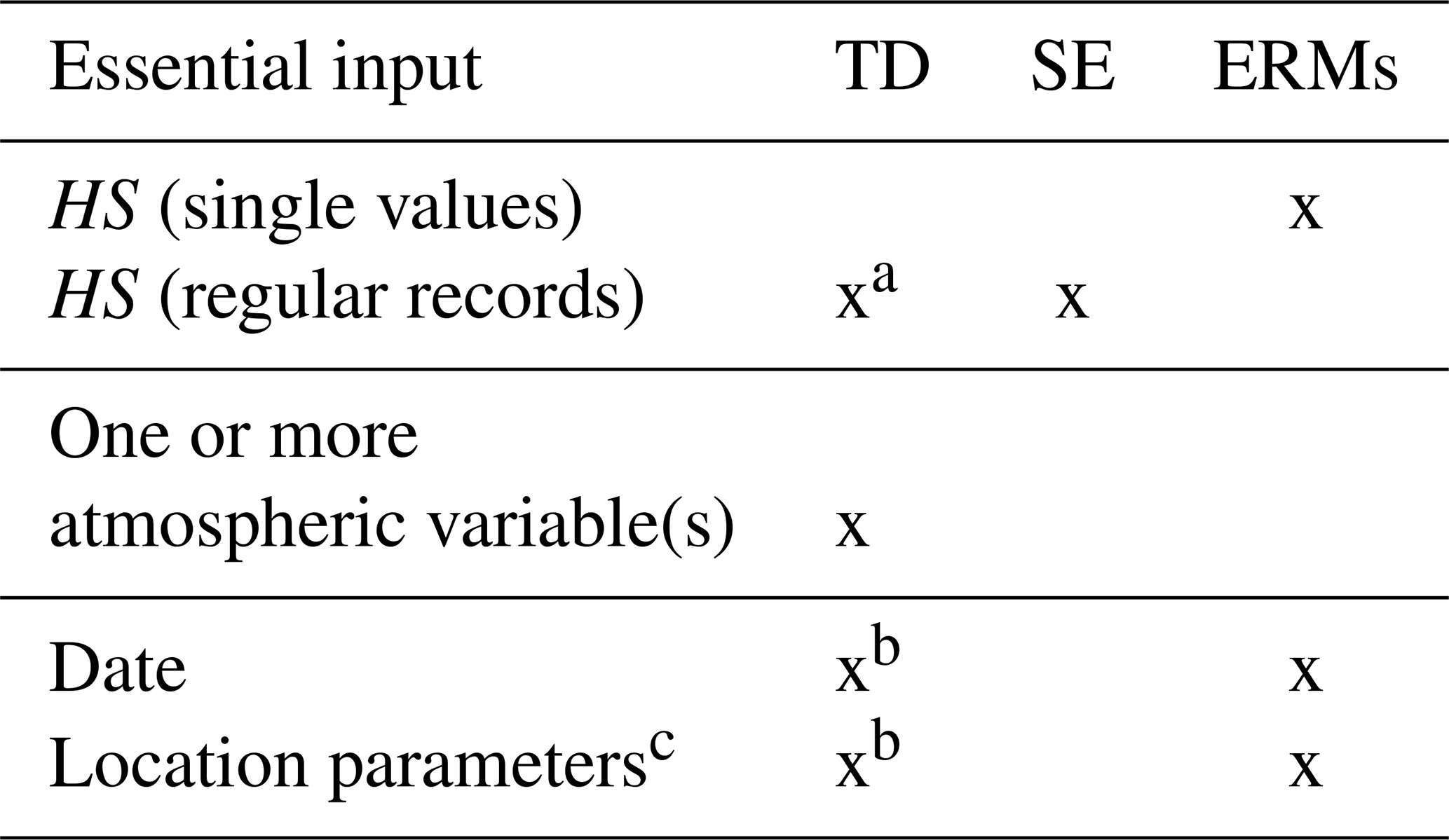
a or another precipitation input; b only essential in some cases, e.g., for parameterizations; c altitude, regional climate, etc.
The semiempirical method of determining SWE presented here maintains the key feature of previous semiempirical models considering only the change of snow depth as a proxy for the various processes altering bulk snow density and snow water equivalent, but it further
-
bases its (dry) snow densification function on Newtonian viscosity;
-
provides a way to deal with small discrepancies between model and observation (on the order of HS measurement errors);
-
takes into account unsteady compaction of underlying, older snow layers due to overburden snow loads; and
-
densifies snow layers from top to bottom during melting phases without automatically modeling mass loss due to runoff.
The ideas for the last three advancements are taken from Gruber (2014), who described them but did not suitably include them as a model. The new modeling approach is named Δsnow. Its code is available as niXmass package in R (R Core Team, 2019), which also includes other models that use snow depth and its temporal change (nix… Latin for snow) to simulate SWE (i.e., snow mass).
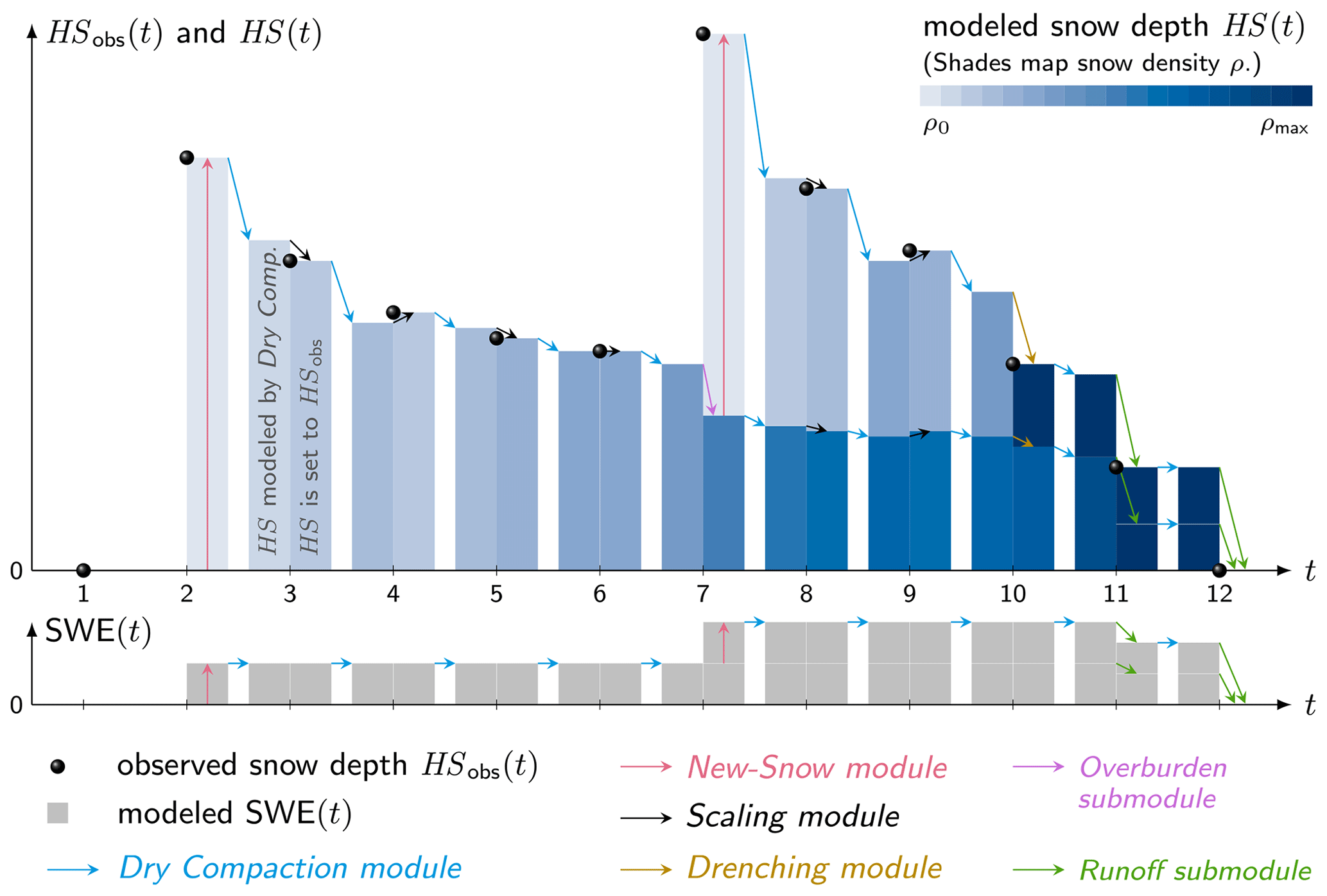
Table 2Summary of compaction processes and processes forcing mass changes that are integrated in Δsnow, as well as processes that are ignored.
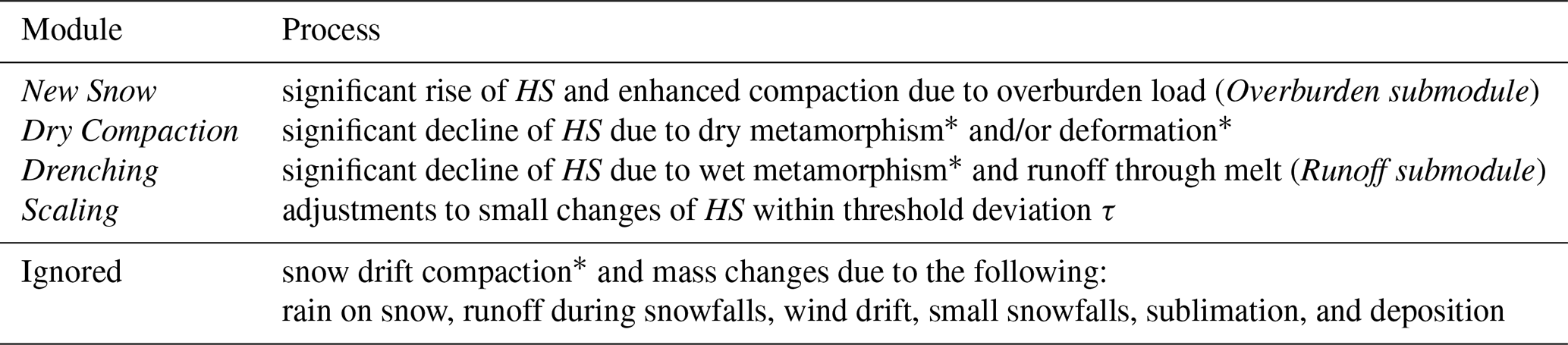
* Terminology follows Jordan et al. (2010).
Snow compacts over time due to various processes. Jordan et al. (2010) categorize them in snow drift, dry and wet metamorphism, and deformation. The Δsnow model cannot deal with snow drift; however, it differentiates between the other processes. Table 2 shows the processes modeled and their corresponding Δsnow modules and outlines the processes that are ignored. The specific modules are described in Sect. 2.2 and 2.3, and a schematic of the model is shown in Fig. 1.
2.1 Preliminary: the first snow layer
For nonzero snow depth observations (HSobs>0) after a snow-free period, the following features are assigned to the Δsnow model snowpack. There is one snow layer (ly=1). Thickness of this model layer (hs) and total model snow depth (HS) are equal and set to observed snow depth: . Analogously, the layer's snow water equivalent equals total snow water equivalent: , with new-snow density ρ0 being an important parameter of the Δsnow model (cf. Sect. 3). The treatment of the first snow event is illustrated at t=2 in Fig. 1.
2.2 Dry Compaction module
Martinec and Rango (1991) used a power function to describe densification of aging snow, because this way errors in initial density ρ0 become less relevant over time. As Δsnow also aims to robustly model SWE of ephemeral snowpacks (e.g., at low-elevation sites) and as overburden load is considered in a particular way (Sect. 2.3.1), it is not expedient to have a direct dependence between density and age of a layer. Instead of a power law, Δsnow (like most modern snow models) simulates snow compaction by way of Newtonian viscosity with associated exponential densification over time (e.g., Jordan et al., 2010). In the Dry Compaction module, the densifying effects of dry metamorphism and deformation are combined, by adopting the relations of Sturm and Holmgren (1998) and De Michele et al. (2013):
t and t−1 are the points in time of the actual and the preceding snow depth observation, respectively. The time span between these measurements is Δt, which is in general arbitrary, but usually it is taken to be 1 d. hs(i,t) is the actual modeled thickness of the ith snow layer. The actual depth of the total snowpack is .
The individual snow water equivalents of the layers are given by swe(i,t), and their sum represents total mass of the snowpack . The vertical stress at the bottom of layer i is given by (De Michele et al., 2013). It is induced by the sum of loads overlying layer i, with ly(t) being the total number of snow layers.
The Newtonian viscosity of snow η is made density-dependent in the framework of the Δsnow model (following Kojima, 1967), but dependencies on temperature or grain characteristics are consciously ignored – due to the lack of information on it when dealing with pure snow depth data. The actual density of layer i is ρ(i,t); it equals ; k and η0 are tuning parameters of the Dry Compaction module (see Sect. 3).
To avoid excessive compaction, a crucial parameter is introduced in Δsnow, as was done by Rohrer and Braun (1994): ρmax. It defines the maximal possible density of a snow layer and, consequently, also the maximum bulk snow density. Finding its optimal value for Δsnow is subject to calibration (Sect. 2.4).
According to Eq. (1), the rate of densification of a certain snow layer is linearly dependent on the overlying snow load and exponentially dependent on the layer's density ρ(i,t). Sturm and Holmgren (1998) conclude that this difference is one reason why “snow load plays a more limited role in determining the compaction behavior than grain and bond characteristics and temperature”. Equation (1) links the densification rate to the layer age (but indirectly by the use of density) and not directly as it was the case with the power-law approach by Martinec and Rango (1991). Consequently, Δsnow's compaction is not directly dependent on layer age, which is a prerequisite for the functioning of the Overburden submodule (Sect. 2.3.1).
The Dry Compaction module is illustrated by the light blue arrows in Fig. 1. This module is applied at every point in time (except if there is no snow; see t=1 in Fig. 1). It is the core module as its output determines the subsequent process decisions and which module will be applied.
2.3 Process decisions
At every point in time, after the Dry Compaction module is run, observed HSobs(t) and modeled HS(t) are compared. The Δsnow's process decision algorithm confronts the difference with τ [m]. τ is another tuning parameter of Δsnow (see Sect. 2.4). Technically, τ is a threshold deviation and defines a limit of ΔHS(t) whose overshooting, adherence, and undershooting heads for one of the modules described in the following Sect. 2.3.1 to 2.3.3. Table 2 links them to snow physics.
2.3.1 New-Snow module
In the case of , meaning observed snow depth is significantly higher than modeled snow depth, a new-snow event is assumed to have occurred, and a new top snow layer is modeled (see at t=2 and t=7 in Fig. 1). Other models have implemented this mechanism (e.g., Martinec and Rango, 1991; Sturm et al., 2010). However, Δsnow goes further and explicitly models the effect of overburden load on underlying layers, defined as their enhanced densification due to stress, which is applied by the weight of new snow. Grain bonds get broken; grains slide, partially melt, and warp (Jordan et al., 2010); and the layers densify comparatively rapidly and strongly. Δsnow interprets overburden load as an “unsteady and discontinuous” stress on the snowpack, under which snow presumably does not react as a viscous Newtonian fluid. As long as the time between two consecutive observations, Δt, is on the order of at least some hours, discontinuity is an intrinsic feature of the process.
The New Snow module realizes the effect of overburden load through the Overburden submodule by reducing each layer's thickness, hs(i,t), using the dimensionless “overburden strain”, ϵ(i,t), defined as
cov [Pa−1] is another tuning parameter of the model (see Sect. 2.4) and controls the importance of the unsteady compaction due to overburden load. According to Sturm and Holmgren (1998) (and in consistency with Eq. 1) snow load has a linear effect on the bulk density. Therefore, ϵ(i,t) is a linear function depending on the load, applied by the overlying new snow on the underlying layers. This load is well approximated by σ0 [Pa]; the larger the overburden load, the stronger the compaction. (The overburden load does not fully equal σ0, since ΔHS(t) is not the depth of the new snow, but it is the difference between modeled depth “before” knowing about the new-snow event and observed depth “after” the new-snow event. An iterative calculation would be more precise; however, Eq. (2) proved to be an adequate compromise between simplicity and accuracy.) In order to avoid , cov is restricted at least to the range of values between 0 and the minimum value of the data record for . As σ0 hardly ever exceeds 1000 Pa, normally is larger than Pa−1. This value marks an upper bound for cov (Sect. 2.4). Dimensionless kov controls the role of a certain snow layer's density on ϵ(i,t) and has to be specified by calibration (see Sect. 2.4). The density dependence of ϵ(i,t) was chosen to be exponential and is constrained by ρmax.
The “overburden strain” ϵ(i,t) theoretically lies between 0 and 1 and compresses all snow layers of the model in the case of a new-snow event. Practically, ϵ(i,t) is often close to zero (in this study 90 % of all computed ϵ values are smaller than 0.09) and extremely rarely higher than 0.3 (in this study only 9 out of 10 000).
The intermediate snow layer thicknesses are and . The compressed layer's masses, swe(i,t), remain unaffected during this process. A new-snow event, identified by the condition , of course not only impacts the older snow and compacts it more strongly but also adds a new-snow layer and mass to the snowpack (pink arrow at t=2 and t=7 in Fig. 1). The following attributes are given to the new layer: and , and the total snow water equivalent arises: . The model snowpack with its new properties is subsequently compacted according to Eq. (1), and the process decision starts again as described in Sect. 2.3. The Overburden submodule is illustrated with a purple arrow at t=7 in Fig. 1.
2.3.2 Scaling module
Equations (1) and (2) are highly simplified representations of the complex viscoelastic behavior of snow, and available HS observations typically only show an accuracy of a few centimeters. The Δsnow model accepts these inherent inaccuracies by not applying too strict criteria in the process decisions described in Sect. 2.3. The threshold deviation τ acts as a buffer to avoid too frequent gain or loss of mass: in the case of , the snowpack does not lose mass nor gain mass, but mass is kept constant. In order to benefit from having a new measurement at every point in time, HS(t) is intentionally set to HSobs(t) by the Scaling module.
The Scaling module forces a partial revaluation of the previous compaction, which was modeled by the Dry Compaction module between t−1 and t. The best-fitted parameter setting for η0 is temporarily rejected and substituted by . It would be straightforward to use one adjusted for all layers. However, this leads to multiple solutions for , making it necessary to calculate different for each layer i. See Appendix B for details on that.
is then used instead of η0 in Eq. (1) to recalculate the compaction of individual layers. HS(t) now equals HSobs(t). In most cases all layers get slightly more or slightly less compacted by the Scaling module than by the Dry Compaction module. Only at rare occasions the scaling does not lead to a compaction but to a small stretching of the snowpack. This only happens if there was a small increase in observed snow depth and very little modeled dry metamorphic compaction; the condition has to be fulfilled. Of course, such stretching does not occur in reality, but also in the model it occurs only rarely and at small scale: in any case the stretching is smaller than τ. The issue is accepted as a model artifact, not least because the stretching enables the very valuable adjustment to HSobs at every point in time without forcing mass gains for insignificant HS raises within the measurement accuracy.
In the case when the density of an individual layer exceeds ρmax by the scaling process, the excess mass is distributed layerwise from top to bottom. SWE remains constant during scaling, unless it would be necessary to compact all layers beyond ρmax. In this case, the appropriate excess mass is taken from the model snowpack and interpreted as runoff, SWE is reduced and all layer thicknesses are cut accordingly (see Runoff submodule in Sect. 2.3.3 for details). As τ turns out to be reasonably chosen on the order of a few centimeters by calibration (Sect. 3), the resulting reduction of SWE within the Scaling module is always quite small: for example, with τ=2 cm and maximum density chosen as 450 kg m−3 (like Rohrer and Braun, 1994), the mass loss due to runoff is only 9 kg m−2.
The Scaling module is illustrated as black arrows in Fig. 1. Note that the scaling is nothing physical but also nothing substantial in terms of SWE, yet it is a way to utilize the advantage of having a measured snow depth at every point in time.
2.3.3 Drenching module
The Drenching module simulates compaction due to liquid water percolating from top to bottom through the snowpack, loosening grain bonds and leading to densification (wet snow metamorphism). In the case when observed snow depth at a certain point in time is significantly lower than modeled snow depth (), the Drenching module is activated.
Δsnow ignores rain on snow since it concentrates on modeling SWE for pure snow depth records without having any further information on, for example, precipitation, temperature, and snowfall level. Possibilities of how rain could be addressed in future developments are outlined in Sect. 4.6.
Table 3The seven parameters of Δsnow. The last column depicts model sensitivity to changes in the density parameters. The respective gradients [kg m−2 per kg m−3] are means over the whole calibration ranges.
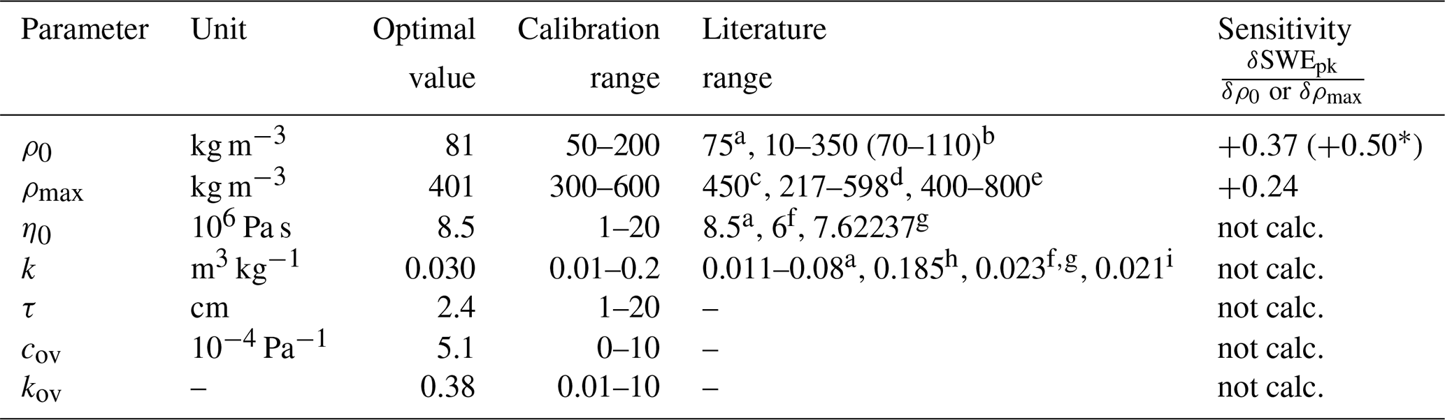
a Sturm and Holmgren (1998), b Helfricht et al. (2018) with range for means in brackets, c Rohrer and Braun (1994), d Sturm et al. (2010), e Cuffey and Paterson (2010), f Jordan et al. (2010), g Vionnet et al. (2012), h Keeler (1969), i Jordan (1991). See Sect. 2.4 for more details. * The value in brackets is the gradient taken from the smaller window between 70 and 90 kg m−3 (cf. Sect. 4.1).
To cope with the model–observation discrepancy , the Drenching module densifies the model layers until ρmax is reached, starting from the uppermost one. Figuratively spoken, a certain layer gets drenched until saturation and meltwater is further distributed to the underlying layer. This process is repeated until transient HS* equals HSobs(t). One or more layers might reach ρmax. In the case when ΔHS(t) is so negative that all model snow layers are compacted and densified to ρmax but still , the Runoff submodule is activated, and runoff R(t) is defined as .
All layer thicknesses are cut by a respective portion: . This mechanism does not reduce the total number of layers, but layers potentially get very thin. During the melt season, where most of the runoff is produced, the Runoff submodule is more or less continuously active until HSobs(t)=0 and all the snow has been converted to runoff. For a distinct snowpack from the first snowfall (t1) until getting snow-free again (t2), one has .
In Fig. 1 the Drenching module is shown by the brown arrows and its Runoff submodule by the green arrows.
2.4 Calibration
Δsnow has seven parameters that have to be calibrated: ρ0, ρmax, η0, k, τ, cov, and kov (cf. Table 3). For the first four parameters, one finds suggestions and ranges in the literature:
Sturm and Holmgren (1998) do not address the criticality for the choice of new-snow density; however, they use constant ρ0=75 kg m−3. It is a well-known characteristic of new snow to show large variations in densities. Helfricht et al. (2018) reviewed many studies and give a general range of 10–350 kg m−3, narrowing it down to “mean values” between 70–110 kg m−3. Note that this is daily densities. Subdaily means of new-snow densities are lower. Helfricht et al. (2018), for example, come up with an average of 68 kg m−3 for hourly time intervals. During the calibration process for the Δsnow model, ρ0 was varied from 50 to 200 kg m−3.
The second density-related calibration parameter is ρmax, which is the maximum possible density within the model framework. Rohrer and Braun (1994) set such a maximum at 450 kg m−3. Sturm et al. (2010) defined it for five different climate classes, ranging from 217 to 598 kg m−3. Glaciologists consider the density at which snow transitions to firn to span 400 to 800 kg m−3 (e.g., Cuffey and Paterson, 2010). Still, manual density measurements of seasonal snow used in previous studies hardly ever exceed 500 kg m−3 (e.g., Jonas et al., 2009; Guyennon et al., 2019). Armstrong and Brun (2010) limit it to approximately 400 to 500 kg m−3 too. In order to find the best value for ρmax used in Δsnow, it was varied from 300 to 600 kg m−3.
Equation (1) needs η0, the “viscosity at [which] ρ equals zero” (Sturm and Holmgren, 1998). It is found to be on the order of 8.5×10⁶ Pa s (Sturm and Holmgren, 1998), 6×10⁶ Pa s (Jordan et al., 2010), and 7.62237×10⁶ Pa s (Vionnet et al., 2012). During the calibration process for the Δsnow model, η0 was varied from 1 to 20×106 Pa s. Parameter k, the second necessary parameter in Eq. (1), was varied from 0.011 to 0.08 m3 kg−1 by Sturm and Holmgren (1998) depending on climate region and respective different types of snow. However, they cite Keeler (1969) in their Table 2 with values for k for “Alpine-new” snow of up to 0.185 m3 kg−1. In more complex snow models k is set to 0.023 m3 kg−1 (see Crocus: bη in Eq. (7) by Vionnet et al. (2012); and also in Eq. (2.11) of Jordan et al., 2010) or 0.021 m3 kg−1 (see SNTHERM: Eq. (29) in Jordan, 1991). Its range for the Δsnow model calibration was set from 0.01 to 0.2 m3 kg−1.
There are no references for the latter three parameters. Threshold deviation τ, as mentioned, might be interpreted as a measure of observation error, is regarded to be on the order of a few centimeters, and was modified from 1 to 20 cm for calibration. The last two parameters, cov and kov, determine the role of overburden strain and are newly introduced in the Δsnow model. At least the limits of cov could be defined (Sect. 2.3.1) as ; kov is only known to be a dimensionless, real, positive number. For calibrating Δsnow, cov and kov were restrained by [0, 10−3 Pa−1] and [0.01, 10], respectively.
The calibration performed in this study is based on Δt=1 d, but longer as well as shorter Δt values are conceivable and could be handled by the Δsnow model too. Note, however, that at least some calibration parameters will change significantly when changing Δt. This gets obvious when considering new-snow density ρ0, which of course is different if defined for 1 h or for a 3 d time step. The usage of this publication's calibration parameters can, therefore, only be suggested for daily snow depth records.
2.4.1 Calibration data and method
The calibration process needs SWE data, which are quite rare per se (see Sect. 1), and regular snow depth records from the same places. There are surprisingly few places where both parameters have been consequently observed side by side for many years, e.g., daily HS measurements accompanied by weekly, biweekly, or monthly SWE measurements.
Gruber (2014) collected 14 years of weekly SWE data from six stations in the Eastern Alps, measured by the observers of the Hydrographic Service of Tyrol (Austria) between winters 1998/99 and 2011/12. The measurements of snow depth and water equivalent were made manually in snow pits with rulers and snow sampling cylinders (500 cm3), respectively. The sites range from 590 to 1650 m altitude and are situated in relatively dry, inner-alpine regions as well as in the Northern Alps and Southern Alps, which are more humid due to orographic enhancement of precipitation (see Gruber, 2014, for details). The sites in the Southern Alps even show a moderate maritime influence due to their vicinity to the Mediterranean Sea, which is the most important source of moisture for this region (e.g., Seibert et al., 2007). These winter seasons cover 1166 measured HS–SWE pairs. Besides these SWE measurements, manual HS measurements are available for every day at the respective stations. Figure A1 and Table A1 provide a map and a list, respectively.
The second source for SWE measurements used for calibration is Marty (2017). The Swiss SLF (Institute for Snow and Avalanche Research) freely provides biweekly SWE and daily HS data from 11 stations in Switzerland. The HS measurements, accompanying the biweekly SWE measurements, were compared with the contemporary value of the daily HS records. Only those sites and years where and when the respective values of the daily HS record match the values of the biweekly measurements were used for calibration. If this condition is fulfilled, it is supposed that SWE and HS measurements fit together sufficiently well, although they unfortunately cannot always be taken exactly at the same place, which introduces uncertainty (e.g., López-Moreno et al., 2020). Consequently, nine stations were used, most of them in the Northern Alps, some inner-alpine, spanning an altitude range from 1200 to 1780 m, with all in all 56 winters and 363 pairs of HS and SWE measurements. Details are given in Fig. A1 and Table A1. Other stations and years suffer from discrepancies caused by too far spatial distances between the measurements and so on.
In order to ensure an unperturbed validation, the observation datasets from Austria and Switzerland (1529 SWE–HS pairs) were split into two almost equally big halves: one for model calibration (SWEcal) and one for validation (SWEval). The two data sources (Gruber, 2014; Marty, 2017) do not address the accuracy of the manual SWE observations. Mostly, SWE measurements made with snow sampling cylinders are used as references in comparison studies, without addressing their accuracy (e.g., Sturm et al., 2010; Dixon and Boon, 2012; Kinar and Pomeroy, 2015; Leppänen et al., 2018). López-Moreno et al. (2020) provide a reported range of 3 %–13 % and condense the results of their own experiments to an error range of 10 %–15 % for bulk snow density. The majority of SWEcal and SWEval comes from the Hydrographic Service of Tyrol, Austria, where snow sampling cylinders (500 cm3) are used (Sect. 2.4.1). The repeatability of this kind of measurement is estimated at ±4 % for glacier mass balance studies (Rainer Prinz, University of Innsbruck, Austria, personal communication, 2020). Roughly interpreting these density measurement “variabilities” as relative observation errors for SWE, the results for absolute accuracy would typically spread across the wide range of about 2 to 50 kg m−2.
Model calibration was performed with the statistical software R (R Core Team, 2019) and the R package optimx (Nash, 2014). Results were obtained with optimization methods L-BFGS-B (Byrd et al., 1995) followed by bobyqa (Powell, 2009), which both are able to handle lower and upper bound constraints. The function to be minimized was the root mean square error (RMSE) of SWEs from the Δsnow model and observed SWEs, using the calibration dataset SWEcal.
This section evaluates the ability of Δsnow to calculate snow water equivalents exclusively from snow depths, as well as its practicability. Table 3 gives an overview of all parameters and summarizes the optimal setting for Δsnow. A discussion of the best-fitted values and of the model sensitivity to parameter changes can be found in Sect. 4.
The minimal RMSE between all SWE observations used for calibration (SWEcal) and the respective modeled values were reached for new-snow density ρ0=81 kg m−3, maximum density ρmax=401 kg m−3, viscosity parameters Pa s and k=0.030 m3 kg−1, threshold deviation τ=2.4 cm, and overburden parameters Pa−1 and kov=0.38.
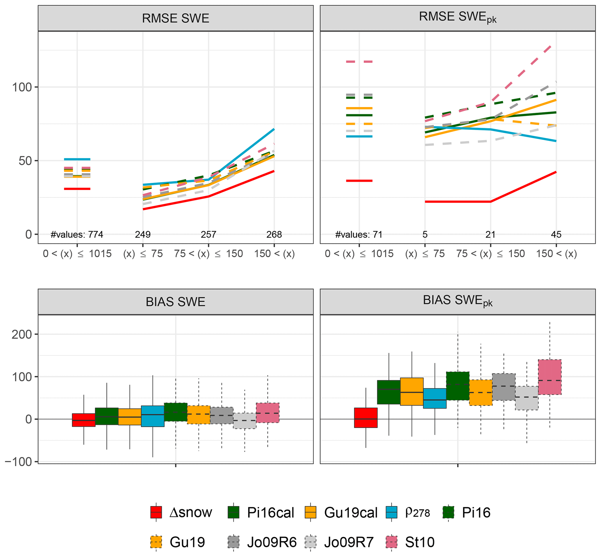
Figure 2Root mean square errors (RMSE) and biases (BIAS) between the Δsnow model and different empirical regression models from the SWEval observations. The Δsnow model, models by Pistocchi (2016) and Guyennon et al. (2019), and the “constant density approach” were calibrated with SWEcal data (Δsnow, Pi16cal, Gu19cal, ρ278; upper panels, solid lines). Dashed lines indicate the Pistocchi (2016), the Guyennon et al. (2019), the Jonas et al. (2009), and the Sturm et al. (2010) models with their standard parameters (Pi16, Gu19, Jo09R6, Jo09R7, and St10). Jo09R6 and Jo09R7 together illustrate the maximum possible spread of the Jonas et al. (2009) model since Region 6 (R6) and Region 7 (R7) are characterized by the highest and lowest “region-specific offset”, respectively. The upper left panel shows RMSEs for all SWEval values (short horizontal lines) as well as for three SWE classes: SWE≤75, SWE>150, and intermediate. Analogously for SWEpk (upper right panel), RMSEs are shown. The boxes for the biases (lower panels) encompass 774 values (left panel, SWE) and 71 values (right panel, SWEpk) and spread from the 25 % to the 75 % quantiles; the whiskers indicate 1.5 times the interquartile range. Units are kg m−2.
3.1 Validation and comparison to other models
In this study no quantitative comparison with thermodynamic snow models was performed, since they need further meteorological data and the focus was on data records constrained to snow depths. However, the Δsnow model was thoroughly evaluated against ERMs. Figure 2 and Table 4 show the results. Even though ERMs do not need meteorological data, it is not straightforward to calibrate them for new sites and applications. From the vast number of ERMs (cf. Avanzi et al., 2015), the ones of Pistocchi (2016) and Guyennon et al. (2019) were chosen to be fitted to SWEcal. These models are quite new and easy to calibrate. Additionally, an approach simply using a constant bulk snow density at every point in time was calibrated to fit this study's data. Thus, 278 kg m−3 turned out to be the optimal value minimizing root mean square errors of all SWEcal values. Moreover, Jonas et al. (2009) and Sturm et al. (2010) were used for comparison. Unfortunately, calibration of these powerful models would have needed much more data than the 780 SWE–HS pairs of the SWEcal dataset. Therefore, Jonas et al. (2009) and Sturm et al. (2010) were used with their standard parameters, but for Jonas et al. (2009) it was distinguished between regions (see the caption of Fig. 2). Other contemporary approaches had to be ignored, mostly because of the problematic transferability of regional parameters (e.g., McCreight and Small, 2014, or Mizukami and Perica, 2008).
Guyennon et al. (2019)Jonas et al. (2009)Sturm et al. (2010)Vionnet et al. (2012)Langlois et al. (2009)Egli et al. (2009)Wever et al. (2015)Sandells et al. (2012)Essery et al. (2013)Table 4Overview on SWE accuracies of different models and studies. The numbers in brackets represent the results for the example portrayed in Figs. 3 and 4 from station Kössen in 2008/09. Units are kg m−2, TD is short for thermodynamic snow models. For model abbreviations, see caption of Fig. 2.

a This is not RMSE of SWEpk but RMSE “from establishment of snowpack to SWEpk”. b See Table 10 in Essery et al. (2013): RMSE for up to 1700 uncalibrated and calibrated simulations.
The bias of modeled SWE (lower left panel in Fig. 2) is quite low and tends to be positive, meaning SWE is often slightly overestimated by the ERMs. Δsnow slightly underestimates SWE on average, with a median bias of −3.0 kg m−2. The overall good results for the ERMs is not surprising, since they are dedicated to perform well on average. The specially calibrated versions of Pistocchi (2016) and Guyennon et al. (2019) show a significantly smaller bias than their originals. The model of Jonas et al. (2009) has the smallest bias for their “Region 7”, encompassing the dry, inner-alpine Engadin as well as parts of the Southern Alps and the very east of Switzerland (Samnaun), which is partly influenced by orographic precipitation from northwesterly flows. In terms of heterogeneity in precipitation climate, “Region 7” is comparable to the region where the SWE data of this study come from.
The other three indicators illustrated in Fig. 2 and summarized in Table 4 show the improved performance of Δsnow compared to ERMs: the latter are intrinsically tied to snow depth (see Sect. 1.2) and are systematically forced to overestimate SWEpk. Note that the maximal SWE of a winter season does not necessarily equal the highest measured SWE, because measurements are only taken weekly or biweekly. In the vast majority of the SWE records used for this study, the highest seasonal observation is followed by at least one lower SWE reading. Sometimes real SWE might be higher after the highest measurement of a winter season was taken, but a thorough data check revealed that this is of minor importance here. It is sufficiently precise to assume that measured seasonal maximum SWE equals SWEpk; Δsnow's bias of SWEpk is very minor, only +0.3 kg m−2. Moreover, the Δsnow model works better for the timing of SWEpk (not shown in Fig. 2 and Table 4). ERMs tend to model SWEpk some days too early, because the date of modeled SWEpk is shifted towards the date of highest HS (cf. Fig. 4).
Another satisfactory validation result for Δsnow is shown in the upper panels of Fig. 2. RMSEs for all SWE values are constantly lower than if modeled with ERMs: an RMSE of 30.8 kg m−2 (Δsnow) contrasts RMSEs between 39.1 and 50.9 kg m−2 (ERMs). Calibrating the models of Pistocchi (2016) and Guyennon et al. (2019) results in some improvement; at least they perform much better than the “constant density approach” after the calibration. The model of Jonas et al. (2009) does a decent job even without recalibration. The method by Sturm et al. (2010) is calibrated with data from the Rocky Mountains. For this comparison, the “alpine” parameters of Sturm et al. (2010) were taken; however, conditions might differ too much from the European Alps. Absolute errors in SWE increase with increasing SWE. For snowpacks lighter than 75 kg m−2, Δsnow's RMSE is 17 kg m−2, between 75 and 150 kg m−2 it is 26 kg m−2, and for snowpacks heavier than 150 kg m−2 it increases to 43 kg m−2.
The Δsnow model also has a small RMSE of 36.3 kg m−2 when modeling SWEpk (Fig. 2, upper right; Table 4, last two columns). Also the SWEpk RMSEs for the different SWE classes are very close to those for SWE, which emphasizes Δsnow's ability to model all individual SWEs comparably well. The evaluated ERMs have much higher, mostly at least doubled, errors in simulated SWEpk. Remarkably, the simple ρ278 approach performs relatively well. In the case when the Jonas et al. (2009) model is suitably adjusted to regional specialties, it performs better than the other ERMs but still significantly worse than Δsnow.
These results demonstrate that Δsnow outperforms ERMs. This can be argued on the basis of Fig. 2 but even more when looking at the ERM studies themselves: Jonas et al. (2009) provide RMSEs between 50.9 and 53.2 kg m−2 for their standard model, which are quite high values compared to the findings of the study in hand (39.4 kg m−2 for their Region 7; see Table 4). One explanation could be that Jonas et al. (2009) as well as other ERM studies rely on a huge amount of (but still diverse measurements in terms of record length) observations per season. The Δsnow model study only consists of data from selected stations with long and regular SWE readings, where also ERMs seem to work better. Guyennon et al. (2019) summarize their and other studies' validation results using MAE, the mean absolute error. Sturm et al. (2010) assess the bias for their “alpine” model at +29 kg m−2 with a standard deviation of 57 kg m−2, and they outline that “in a test against extensive Canadian data, 90 % of the computed SWE values fell within ±80 kg m−2 of measured values”. Table 4 provides an overview and shows that ERMs generally perform better with this study's data than with their original data.
3.2 Illustration
Figure 1 schematically shows the functioning of the Δsnow model. A practical example is provided in Fig. 3, based on the optimal calibration parameters found during this study. Kössen, the station shown, is situated in the Northern Alps at 590 m (cf. Fig. A1). Although it is a low-lying place, it is known to be snowy, which is, firstly, due to intense orographic enhancement of precipitation associated with northwesterly to northeasterly flows in the respective region (Wastl, 2008) and, secondly, comparably frequent inflow of cold continental air masses from northeast. Showing the example of Kössen should emphasize the versatile usability of Δsnow: it is not only designed for high areas with deep, long-lasting snowpacks but also for valleys with shallow, ephemeral snowpacks. Winter 2008/09 was chosen because Δsnow shows a rather typical performance in terms of RMSE and BIAS in Kössen (see Table 4, values in brackets), and because some important, model-intrinsic features can be addressed and discussed:
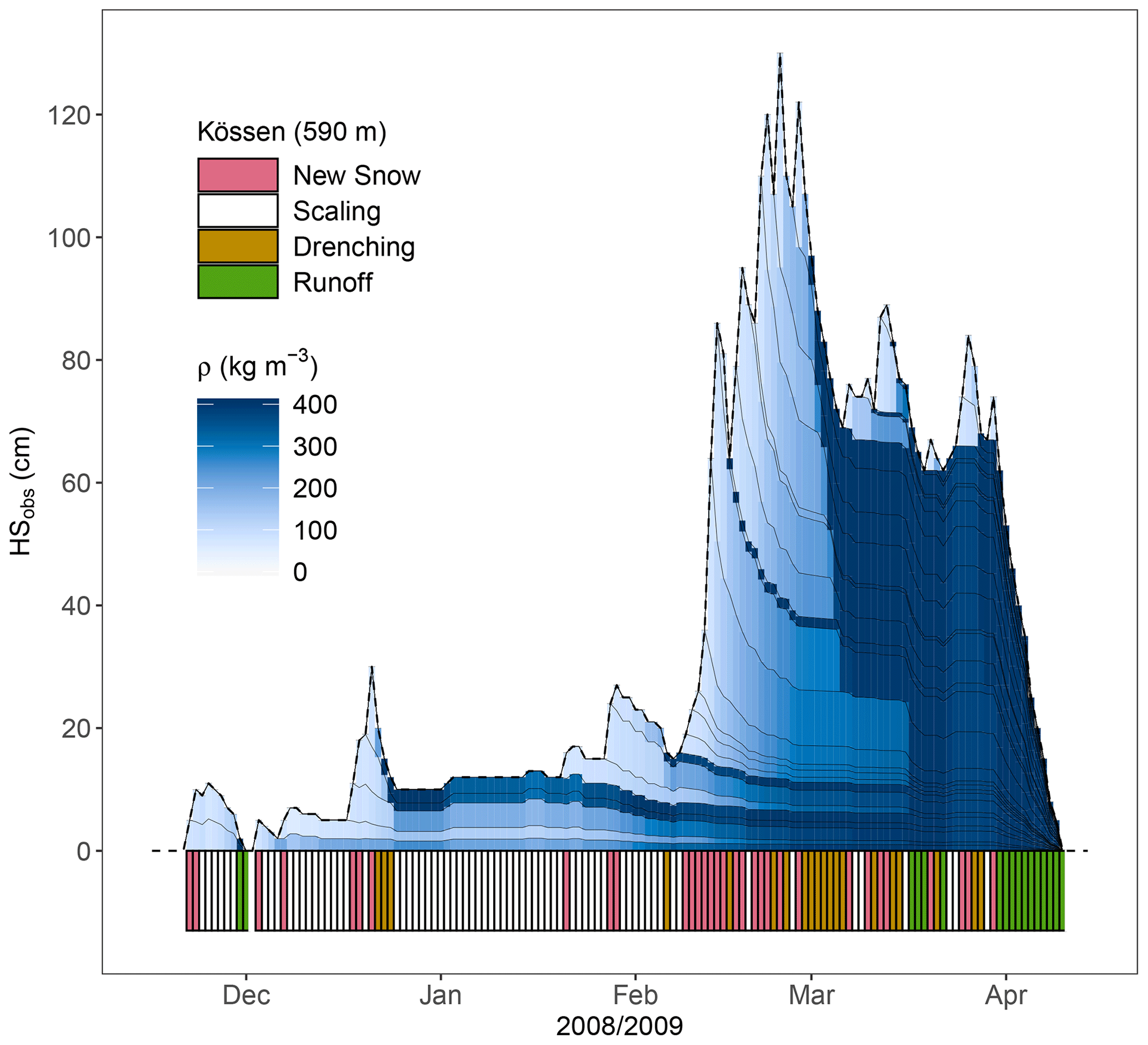
Figure 3Winter of 2008/09 in Kössen (Northern Alps, Austria) portrays density evolution as simulated by the Δsnow model. Respective (sub)modules are depicted in colors at the bottom, whenever activated. Note that Δsnow is not intended to simulate individual layers but to calculate daily SWE, SWEpk, and daily bulk density. Descriptions and discussions of some features are given in the text.
Late November 2008 brought the first, however transient, snowpack of the season (Fig. 3). The Δsnow model identifies 2 d with snowfall (purple markings) and models two respective snow layers, which can be distinguished by the thin black line in Fig. 3. After about a week, the snowpack starts to melt, the snow layers reach ρmax very fast (the blue shading gets dark), and finally all the snow was converted to runoff (green markings). In the second half of December, there were 3 d with new snow, followed by a strong decline in snow depth. In the frame of the Δsnow model, this HS decrease is only possible if the layers “get wet” and the Drenching module is activated (marked in brown). The layers get denser, starting at the top. However, the decrease was “manageable” only by increasing the two uppermost layer densities to ρmax and making the third layer just a bit denser. Not all layers got to ρmax, and no runoff was modeled. The Δsnow model conserves the two dense layers until the end of the winter, which can clearly be seen in Fig. 3. One could interpret the layers as consisting of melt forms or a refrozen crust. However, such interpretations require caution, because modeling detailed layer features is not the intention of Δsnow. During January Fig. 3 shows a phase where modeled values and observations agree to a high extent, and only the Scaling module is activated for small adjustments (white markings). Small “stretching events” can be recognized, e.g., on 2 and 3 January, where model snow layers are set less dense in order to avoid too frequent mass gains. During continuous snowfalls in February the successive darkening of the blue layer shadings illustrates a phase of consequent compaction, which actually lasts until March, when strong decreases in HSobs start to activate the Drenching module. Still, runoff is not yet produced. Only in the second half of March does the whole model snowpack reach ρmax (“saturation”). The ablation phase is clearly distinguishable and lets the snowpack vanish rapidly towards 10 April 2009.
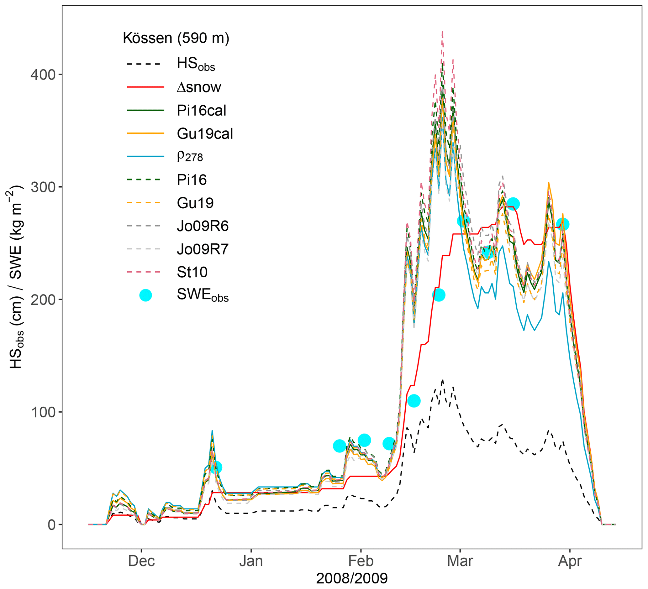
The snow depth record of Kössen from 2008/09 was also used to compare different ERMs and Δsnow to SWE observations (Fig. 4). These measurements (light blue circles) are part of the SWEval sample and were manually made with snow sampling cylinders; one after the December 2008 snowfall and another nine on a nearly weekly basis between late January and late March 2009. Figure 4 also provides various model results, and some respective key values are given in Table 4. Not surprisingly and thus evidently, the ERM SWE curves follow the snow depth curve (black dashed line). The first four measurements are not well simulated by the Δsnow model (red line); the ERMs perform better in this illustrative case. But after the stronger snowfalls of February the picture changes indisputably in favor of the Δsnow model. This is a typical pattern, because ERMs are too strongly tied to snow depth and therefore mostly (1) overestimate SWEpk, (2) model its occurrence too early, and (3) – most importantly – force modeled SWE to reduce during pure compaction phases after snowfalls. Evidently, the ability of Δsnow to conserve mass during the phases with dry metamorphism is its strongest point, not only in Kössen 2008/09 but also on average (cf. Fig. 2 and Table 4).
Model results clearly depend on the parameters. Their optimal values are subject to calibration. The choice of the best-fitted values is rated and discussed in the following Sect. 4.1 to 4.5. Section 4.6 to 4.8 cover possible future developments, accuracy issues, and Δsnow's applicability in remote sensing.
4.1 New-snow density ρ0
Being aware of both the potentially large variations of new-snow density and the possible cruciality of this parameter for SWE simulation by the Δsnow model, ρ0 was chosen to be a constant in the framework of the model. ρ0=81 kg m−3 turned out to be the best choice after calibration with SWEcal. This value clearly lies within the broader frame of possible new-snow densities (Table 3) and quite closely to 75 kg m−3 by Sturm and Holmgren (1998), but it is found in the lower part for typical new-snow densities (e.g., Helfricht et al., 2018). A possible explanation is that the SWE measurement records used for the calibration tend to underrepresent late winter and spring conditions. Regular (weekly, biweekly) observations capture the short melt seasons worse than the longer accumulation phases. Therefore, SWE records might be biased towards early and midwinter new-snow densities, which are lower (e.g., Jonas et al., 2009). Still, there are also some indications that using, for example, 100 kg m−3 as constant for new-snow density when modeling SWE results in an overestimation of precipitation (up to 30 % according to Mair et al., 2016). The calibrated value for ρ0 can be regarded as a reasonable result, even more when only considering it as a model parameter but not as a physical constant.
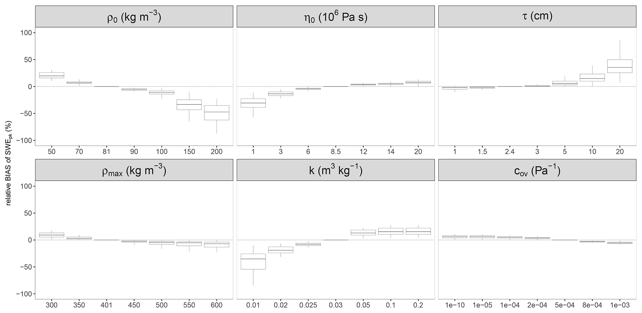
Figure 5Sensitivity of SWEpk to changes in model parameters. The “relative bias of SWEpk” is defined as the difference between SWEpk with best-fitted values and SWEpk with changed parameters (while all others are kept unchanged) divided by the best-fitted SWEpk. The boxes comprise SWEpk of all stations and all years of the validation dataset SWEval (71 values) and display medians as well as 25 % and 75 % percentiles; the whiskers indicate 1.5 times the interquartile range. For details and analysis, see the text.
The sensitivity analysis illustrated in Fig. 5 confirms the importance of a good choice of ρ0. Increasing ρ0 leads to a decrease of the relative bias of seasonal SWE maxima (SWEpk). Note the definition of the relative bias in the caption of Fig. 5. In absolute values, too small ρ0 values cause too small SWEpk values, while using higher values leads to an overestimation of SWEpk. This behavior supports the above-mentioned tendency to overestimate precipitation when choosing constant 100 kg m−3 as new-snow density. As expected, the new-snow density is the most crucial parameter of the Δsnow model (cf. Table 3). The median relative bias of SWEpk changes by −0.46 % per +1 kg m−3 if the whole calibration range of ρ0 is considered to calculate the sensitivity (50–200 kg m−3). This means a median change in SWEpk of +0.37 kg m−2 when ρ0 is risen by +1 kg m−3. If the limits are restricted more tightly around the optimal value, the gradient is even steeper: −0.62 % and +0.50 kg m−2 per +1 kg m−3, respectively, when the gradient is approximated for the range 70–90 kg m−3. The widely used ρ0 value of 100 kg m−3, consequently, causes a median overestimation of SWEpk of about 12 % in the Δsnow model. Daily SWE shows the same behavior (not shown), and users should be aware of this. The suggestion is to either use the best-fitted parameters of this study or recalibrate all parameters with appropriate SWE data but not to adjust only single parameters. The value of ρ0=81 kg m−3 seems to be a good compromise, at least in alpine areas. However, for maritime, very dry, polar, or tundra regions, the optimized ρ0 should be used with caution.
4.2 Maximum density ρmax
The maximum bulk snow density of a snowpack changes from year to year and site to site. For Δsnow, simplicity and independence from meteorological variables outweigh precision. Even more so when there are good arguments for the existence of a typical maximum bulk density ρmax. Put simply, seasonal and also ephemeral snowpacks melt away when they get water saturated. Before that, there is limited time for dry densification; dry winter snow's bulk density is widely described as staying below about 350 kg m−3 (e.g., Cuffey and Paterson, 2010; Sandells et al., 2012). Accounting for the fact that volumetric liquid water content of about 10 % marks the funicular mode of liquid distribution in old, coarse-grained snow (Denoth, 1982; Mitterer et al., 2011), this leads to the rough estimate of a typical maximum bulk density of about kg m−3. Convincingly, the optimal value for ρmax in the Δsnow model turns out to be 401 kg m−3, which is close to that value and well within the range given in the literature (Table 3). Moreover, this is virtually the same as the median maximum seasonal density of the SWEval data records (400 kg m−3; see box plot in Fig. 6), which is another indication why ρmax could be regarded as a typical seasonal maximum of ρb.
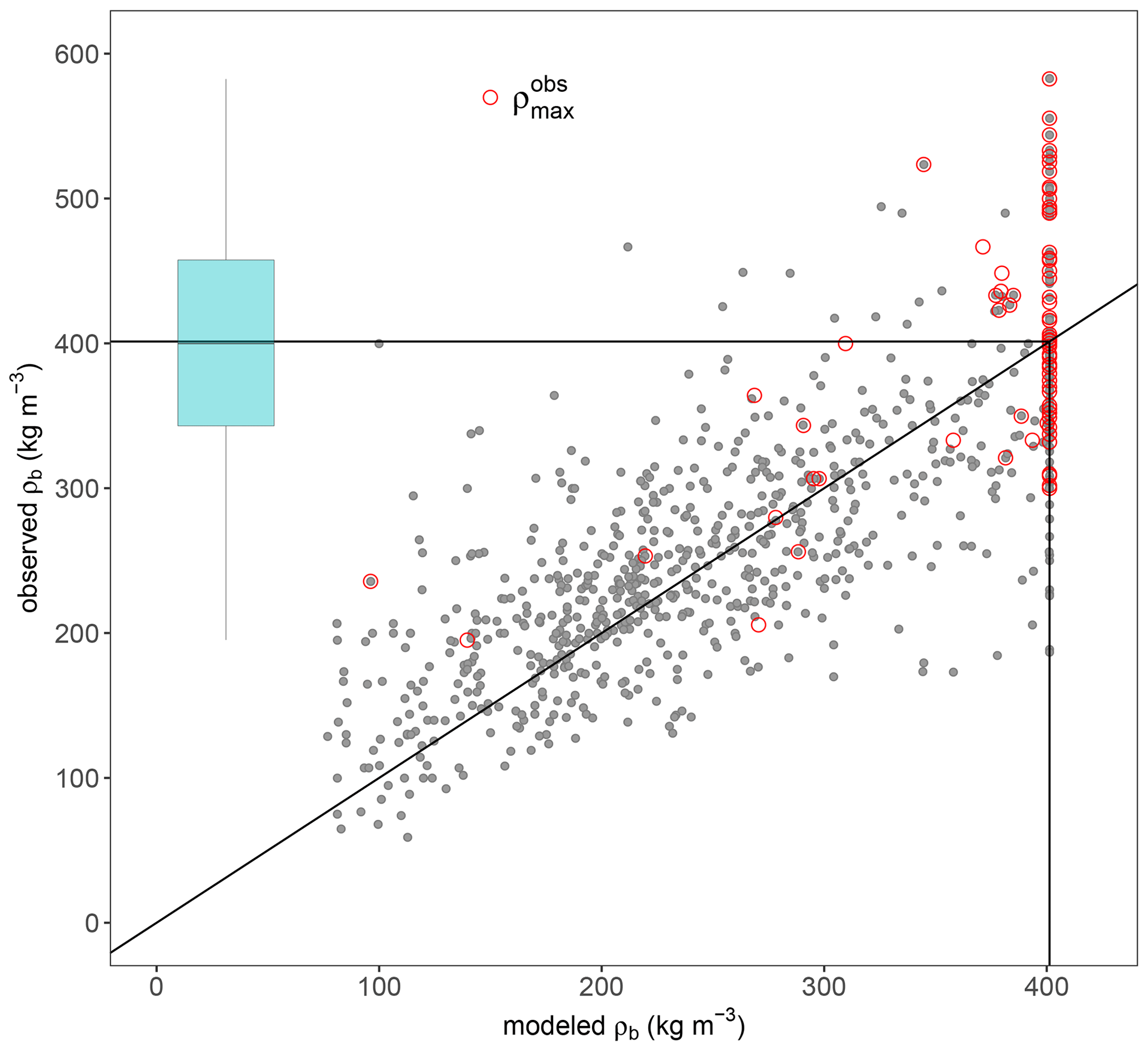
Figure 6Scatter plot of all modeled bulk snow densities ρb versus all observed ρb from the validation dataset. (SWEval, 767 data pairs. Seven observations, which are higher than 600 kg m−3, were ignored.) Red circles reflect the 71 observed yearly maxima (), most of them occur when also modeled snowpack is at ρmax=401 kg m−3. The box plot shows the distribution of with median, 25 % and 75 % percentiles, and whiskers at 1.5 times the interquartile range.
Figure 5 illustrates the similarity between ρ0 and ρmax regarding their influence on SWE simulations. Keeping the other six Δsnow parameters constant but increasing ρmax leads to increased SWEpk and vice versa – just like ρ0. The Δsnow model is not as sensitive to changes in ρmax as it is to changes in ρ0: raising ρmax by +1 kg m−3 leads to a mean decrease of the relative bias of SWEpk of −0.06 %, which corresponds to an increase in absolute SWEpk of +0.24 kg m−2 per +1 kg m−3. We consider the ρmax value of 401 kg m−3 to be representative for Alpine areas as our calibration dataset encompasses the full range of environmental conditions. Be aware that solely changing parameter ρmax for an application of the Δsnow model elsewhere, without proper recalibration of the other parameters, might lead to significant changes in the results for SWE.
4.3 Viscosity parameters η0 and k
Equation (1) represents the settlement and densification function of Δsnow. Two parameters η0 and k act as adjustment screws and have to be calibrated. In this study, best-fitted η0 is 8.5×10⁶ Pa s, and the optimized value for k is 0.030 m3 kg−1. Both values are close to other studies' results and suggestions (Table 3).
As far as Δsnow's sensitivity to changes in the viscosity parameters η0 and k is concerned, Fig. 5 shows that an isolated rise of the model snow viscosity – either by enhancing η0 or k – increases the relative bias of SWEpk, which means a decrease in absolute values of SWEpk. This behavior is consistent, since higher viscosity reduces the densification rate, and the model snowpack tendentiously stays deeper. Consequently, increases in observed snow depth tend to bring less new snow while the New Snow module is run (Sect. 2.3.1). Finally, simulated SWEpk is reduced when η0 or k values are increased and vice versa.
4.4 Threshold deviation τ
Δsnow's parameter to cope with uncertainties in snow depth is τ, and it is considered to be not more than a few centimeters. In particular, it should avoid excessive production of snow mass in the model through too frequent simulation of new-snow events (see Sect. 2.3). τ is kind of a peculiarity of the Δsnow model, and therefore no bounds can be found in literature. It was generously accepted to range between 1 and 20 cm for calibration and turned out to be optimal at τ=2.4 cm (Table 3). Given the wide range of possible values, this is very close to what would be expected as a measure for HSobs accuracy.
Model sensitivity to changes in τ turns out to be quite low for values on the order of a few centimeters, but the influence on simulated SWEpk is strongly increasing if τ is chosen greater than about 5 cm (Fig. 5). This result makes a lot of sense if τ is seen as a measure of observation accuracy, because this is very likely to be better than 5 cm. Like changes in η0 and k, changes in τ are indirectly proportional to changes in SWEpk, for a closely related reason: the bigger τ, the more often small new events are not counted as such, because the Scaling module (Sect. 2.3.2) is more frequently activated at the cost of the New Snow module (Sect. 2.3.1).
4.5 Overburden parameters cov and kov
Aside from τ, there are two more parameters that are peculiar to the Δsnow model. They are needed to simulate unsteady compaction by overburden load of new snow. Because of their presumed uniqueness in the snow model spectrum, there is no information available on how to choose them (see Sect. 2.4). The calibration produces Pa−1 and kov=0.38 as best-fitted values (Table 3).
The sensitivity of modeled SWEpk to changes in either cov or kov are quite minor. (See Fig. 5 for cov; kov is not shown, because it is comparable but of opposite sign.) The reason for this relative insensitivity of the model to changes in cov and kov could be the contradicting effects of these two overburden parameters: higher cov leads to higher SWE and SWEpk, and higher values of kov cause lower SWE.
4.6 Incorporating rain on snow and other possible improvements
In principle, Δsnow could deal with rain-on-snow events. Unsteady compaction due to overburden load, for example, is not restricted to new snow. It could also be triggered by the mass of rain water, both in nature and in the framework of the Δsnow model. Still, the respective feature is not implemented at the moment, because identifying criteria for rain-on-snow events based on pure snow depth records is very problematic and beyond the scope of this paper.
Another eventual future development is the refinement of the density parameters ρ0 and ρmax since, firstly, Δsnow reacts quite sensitively to their changes and, secondly, some relations are well known, e.g., ρ0's dependence on the climatic aridity or ρmax's tendency to increase for aging snow. Setting ρmax to a fixed value of 401 kg m−3 actually disqualifies the Δsnow model for snow older than an estimated 200 d. Additional calibrations could be performed for maritime, very dry, polar, or tundra regions as well as for very long-lasting snowpacks. Note, however, that all of these adaptions introduce more parameters to the Δsnow model and reduce its generality. Benefits should be evaluated critically, and probably this evaluation should start with the overburden load treatment of Δsnow. It is possible that refining the density parameters is more valuable than the special treatment of unsteady compaction due to overburden loads.
4.7 SWE accuracy
Table 4 provides an overview of uncertainties for SWE, also for thermodynamic models: Vionnet et al. (2012) find an RMSE and bias of 39.7 and −17.3 kg m−2, respectively, comparing 1722 manual samplings at Col de Porte (Chartreuse Mountains, France) and Crocus. Wever et al. (2015) and Sandells et al. (2012) come up with RMSEs of about 39.5 kg m−2 (SNOWPACK) and 30–49 kg m−2 (SNOBAL), respectively. Langlois et al. (2009) find more optimistic values, however, based on much fewer data. On the contrary, Egli et al. (2009) give reason to expect higher RMSEs, but their study is exclusively based on data from the snowy, high-altitude station Weissfluhjoch (Switzerland), which intrinsically promotes higher absolute errors. The comprehensive simulation experiment by Essery et al. (2013) results in an RMSE range of 23–77 kg m−2.
As a synopsis of the study in hand, absolute SWE accuracies could be estimated as follows: (1) 2 to 50 kg m−2 for manual measurements, which are widely used as reference, (2) 30 to 40 kg m−2 for thermodynamic models, and (3) 40 to 50 kg m−2 for empirical regression models. In this respect, it is striking to find Δsnow's RMSE at 30.8 kg m−2.
4.8 Application to remote sensing data
Looking at current developments in deriving SWE from snow depths monitored with lidar and photogrammetry, Δsnow might be considered one of the “potential […] other snow density models” (Smyth et al., 2019) that could be included in respective future research. Lidar and photogrammetry have errors on the order of 10 cm (Smyth et al., 2019), typically corresponding to SWE errors of 20 to 40 kg m−2. This is on the order of the Δsnow model errors. Remote-sensing-derived snow depth data are discontinuous through time, but Δsnow could be adapted for that in order to upgrade from a point model to a computationally fast distributed model. A possible combination of Δsnow with modern, large-scale snow depth products like those presented by Lievens et al. (2019) motivates future developments in this direction.
A new method to simulate snow water equivalents (SWEs) is presented. It exclusively needs snow depths and their temporal changes as input, which, given the nature of available data, is its major advantage compared to many other snow models. It is shown that basic snow physics, implemented in a layer model, suffice to better calculate SWE than snow models relying on empirical regressions.
Regular snow depth records are used to stepwise model the evolution of seasonal snowpacks, focusing on their mass (i.e., SWE) and respective load. Snow compaction is assumed to follow Newtonian viscosity, unsteady stress for underlying snow layers by the overburden load of new snow is regarded separately, melted mass is distributed from upper to lower layers, and – eponymous for the model – the measured change in snow depth between two observations is used as a precious corrective by accounting for measurement uncertainties.
The Δsnow model mainly draws on Martinec and Rango (1991) and Sturm and Holmgren (1998) and transforms them to an open-source R code, which is available through https://cran.r-project.org/package=nixmass (last access: 2 March 2021). Δsnow requires only HS as input and does not need meteorological or geographical forcing, although calibration of seven parameters is needed. To provide an optimal setting and utmost applicability, data from 14 climatologically different places in the Swiss and Austrian Alps are utilized. This is challenging, since calibration needs multiyear SWE observations as well as consecutive (e.g., daily) snow depth readings from the same places. Δsnow is calibrated with 67 winters. The validation dataset consists of another 71 independent winters. Whereas calibration is quite complex, the application of the Δsnow model is cheap in terms of computational effort: deriving a 1-year SWE record from 365 snow depth values, for example, only takes a few seconds with today's standard desktop CPUs and can certainly be sped up significantly.
In this study it is argued that Δsnow is situated between sophisticated “thermodynamic snow models”, necessitating meteorological and other inputs, and modest “empirical regression models” (ERMs), relying on simple statistical relations between SWE and snow depth, date, altitude, and region. The key qualities of the Δsnow model are the following.
-
Low complexity: Δsnow is a semiempirical multilayer model with seven parameters. In some respect it is even less demanding than ERMs, because no information on date, altitude, or region is required.
-
High universality: Δsnow simulates individual SWE values – like the important seasonal maximum SWEpk – comparably well as SWE averages.
-
High accuracy: Δsnow's performance in modeling SWE and SWEpk is comparable to thermodynamic models and superior to ERMs. Root mean square errors for SWEpk are 36.3 kg m−2 for Δsnow and about 70 to >100 kg m−2 for ERMs.
As the development of the Δsnow model is application-driven, it provides no new findings in snow physics. Still, Δsnow takes well-known basic snow principles and arranges them in a physically consistent way, while retaining the simplicity of using the single forcing parameter of snow depth. After calibration, the Δsnow model is widely usable and particularly of value for attributing snow water equivalents to all long-term and historic snow depth records, which are so valuable for climatological studies and extreme value analysis for risk assessment of natural hazards.
A map with the stations used for calibration and validation of the Δsnow model is shown in Fig. A1. Table A1 provides details on the stations and the data.
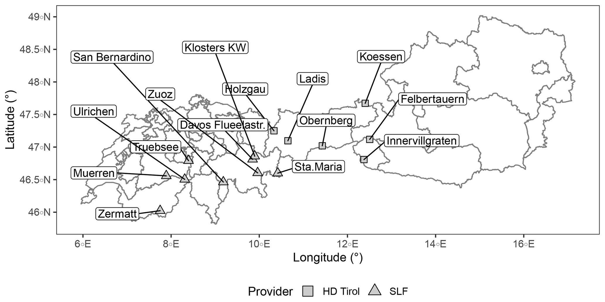
Figure A1Locations of the stations used for calibration and validation. Austrian stations are operated by the Hydrographic Service of Tyrol (HD Tirol), and the Swiss stations by the Swiss Federal Institute for Forest, Snow and Landscape Research (WSL) Institute for Snow and Avalanche Research SLF. See Table A1 and text for more details.
Table A1Overview of stations with daily snow depth records and about weekly or biweekly (Austria or Switzerland) manual SWE observations which were used for calibration and validation. and give the numbers of respective manual SWE observations. Stations nos. 1 to 6 are located in the Austrian province of Tyrol and nos. 5 and 6 are in the subprovince of East Tyrol, which are all operated by the Hydrographic Service of Tyrol. Swiss station nos. 7 to 15 are operated by the WSL Institute for Snow and Avalanche Research SLF. (Compare Fig. A1.) The data sources are Gruber (2014) and Marty (2017).

a Indicated years mark the start of respective winter seasons. b 2006 is missing.
The Scaling module (Sect. 2.3.2) recalculates the viscosity parameter η0. This temporary does not only depend on the point in time t whenever the Scaling module is activated but is also different for each layer i. The reason is described in the following.
The Scaling module aims for the condition that the actual model snow depth HS(t) equals the actual observed snow depth HSobs(t).
It follows from Eq. (1) and substituting that
which is a rational function f of the form
Because f(η) has poles at −x1, …, −xN, the equation f(η)=HSobs has multiple solutions. Consequently, this approach – with being independent from layer i – shows a clear nonphysical behavior making it necessary to calculate different for each layer i based on Eq. (B1):
The solution to this issue in the Scaling module of the Δsnow model is based on the assumption that observed compaction between t−1 and t can be approximated linearly for each layer:
The layer-individual viscosities can be calculated as
Substituting those values for in Eq. (B1) fulfills its precondition, and the modeled equals the observed snow depth. The newly calculated values are different for each layer – in contrast to the fixed η0 defined in Sect. 2.2, which is valid for the whole snowpack (outside the Scaling module). Note that these new viscosities are only used temporarily in the Scaling module. They have no analog in reality and can also have negative values, but they are mathematically sound.
In this section an example is given of how the Δsnow model can be used to attain a map of snow loads in Austria. European Standards (e.g., European Committee for Standardization, 2015) define the “characteristic snow load” sk as the weight of snow on the ground (which is the product of SWE and the gravitational acceleration) with an annual probability of exceedance of 0.02, i.e., a snow load that – on average – is exceeded only once within 50 years. Unfortunately, SWE is not measured on a regular basis at a reasonable number of sites in Austria (and most other countries). The Δsnow model, however, can provide long-term Austrian SWE series from widely available HS series, which can in turn be used for a spatial extreme value model. No other snow model is capable of this in a comparable manner, since either SWEpk is poorly modeled (ERMs) or more meteorological input would be needed (thermodynamic models). Among several possibilities to spatially model snow depth extremes like max-stable processes (see e.g., Blanchet and Davison, 2011), the smooth modeling approach of Blanchet and Lehning (2010) can be used when marginals instead of spatial extremal dependence are in focus.
C1 Smooth modeling
Extremes following a generalized extreme value distribution (GEV; Coles, 2001) with parameters μ, σ, and ξ can be modeled in space by considering linear relations for the three parameters of the form
at location x, where η denotes one of the GEV parameters, y1, …, ym are the considered covariates as smooth functions of the location, and α0, …, αm∈ℝ are the coefficients. Assuming spatially independent stations, the log-likelihood function then reads as
where l only depends on the coefficients of the linear models for the GEV parameters. This approach was termed smooth modeling by Blanchet and Lehning (2010). A smooth spatial model for extreme snow depths in Austria was already presented in Schellander and Hell (2018), using longitude, latitude, altitude, and mean snow depth at 421 stations. Considering the strong correlation between snow depth and snow water equivalent, it would be natural to spatially model SWE extremes in the same manner.
C2 Fitting a spatial extreme value model
For this application, 214 stations with regular snow depth observations in and tightly around Austria of the national weather service (ZAMG, Zentralanstalt für Meteorologie und Geodynamik) and the hydrological services are used. The dataset has undergone quality control by the maintaining institutions and covers altitudes between 118 and 2290 m. The records have lengths of 43 years and cover winters from 1970/71 to 2011/2012.
In a first step the Δsnow model was applied to these snow depth series to achieve 214 data series of SWE across Austria. Then the linear models for the three GEV parameters according to Sect. C1 were defined via a model selection procedure. For that purpose, a generalized linear regression was performed between the parameters and the covariates longitude, latitude, altitude, and mean snow depth, which were added in a stepwise manner. Using the Akaike information criterion (AIC; Akaike, 1974), the best linear model between a given full model (μ∼all covariates) and a null model (μ∼1) with the smallest AIC was selected. Using these models and the covariates of the 214 stations, a smooth spatial model for the yearly maxima of the SWE values was fitted.
C3 Return level map of 50-year snow load in Austria
The spatial extreme value model developed in the previous section was applied to a grid provided by the SNOWGRID climate analysis (Olefs et al., 2013). It offers the necessary covariates longitude, latitude, altitude, and yearly mean snow depths from 1961 to 2016. The grid features a horizontal resolution of 1×1 km. Some minor SNOWGRID pixels have unrealistically large mean snow depth values, arising from a poor implementation of lateral snow redistribution at high altitudes (18 px, i.e., 0.02 % with values between 5 and 65 m). They are masked for the calculation of SWE return level maps. The return level map for a return period of 50 years can be seen in Fig. C1.
As expected, due to the strong correlation of the SWE maxima with mean snow depth, the largest snow loads are located in the mountainous areas of Austria. Although the unrealistic mean snow depth values of SNOWGRID are masked, the model produces a number of 59 (0.06 %) unrealistic snow load values larger than 25 kN m−2 in an altitude range between 1500 and 3700 m. For a model that would be seriously used, for example, in general risk assessment or structural design, this problem could possibly be tackled with a nonlinear relation between SWE maxima and mean snow depth or altitude. This is, however, beyond the scope of this study. Note that in the actual Austrian standard (Austrian Standards Institute, 2018) there are no normative snow load values defined above 1500 m altitude.
All but two locations of the Austrian SWE measurement series that were used for calibration and validation of the Δsnow model (see Sect. 2.4.1) are included in the dataset used to fit the spatial model in Sect. C2. Those two stations, Holzgau and Felbertauern with 14 years of SWE observations each, are used to qualitatively compare (1) the spatial model fitted in Sect. C2, (2) SWE extremes modeled from daily snow depths with the Δsnow model, and (3) extremes computed “directly” from (ca. weekly) observed SWE values. Figure C2 gives an idea of the model performance at stations Holzgau and Felbertauern (see Figs. A1 and C1 for their locations). For the lower-lying station Holzgau (1100 m), all three variants overlap very well. The 50-year return level is 4.65 kN m−2 for the smooth spatial model, 4.72 kN m−2 for Δsnow, and 4.8 kN m−2 for the observations. Note that the last value stems from weekly observations and therefore does not necessarily reflect the true yearly maxima, which naturally must be equal or slightly higher. By the way, the corresponding value of sk from the Austrian snow load standard for Holzgau is 6.3 kN m−2 (Austrian Standards Institute, 2018; accessible online at eHORA, 2006).
For the higher station Felbertauern (1650 m), the agreement between SWE from the Δsnow model and observed values is again very good. However, their GEV fits differ significantly. While the fit to the observations shows a negative shape parameter of , the fit to the values modeled with the Δsnow model gives a positive shape parameter of ξ=0.1, leading to much larger return levels for higher recurrence times. It should be pointed out that the GEV fits based on Δsnow simulations and observations are unreliable, given the short data sample of only 14 yearly maxima. Indeed, by using a sample size of 43 years and borrowing strength from neighboring stations, the spatial model provides the best fit to observations as well as modeled SWE values. The 50-year snow load return values are 6.4 kN m−2 for the spatial model, 6.8 kN m−2 for Δsnow, and 5.7 kN m−2 for the fit to the observations. No normative value is defined for Felbertauern, because it is situated higher than 1500 m (Austrian Standards Institute, 2018).
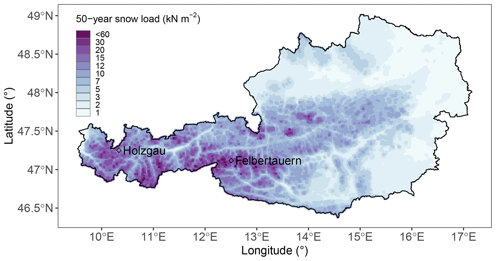
Figure C150-year return levels of snow load in Austria. Two stations with SWE observations are outlined for a qualitative validation. This map is based on 214 snow depth records, Δsnow-derived SWE, and smooth spatial modeling of their extremes.
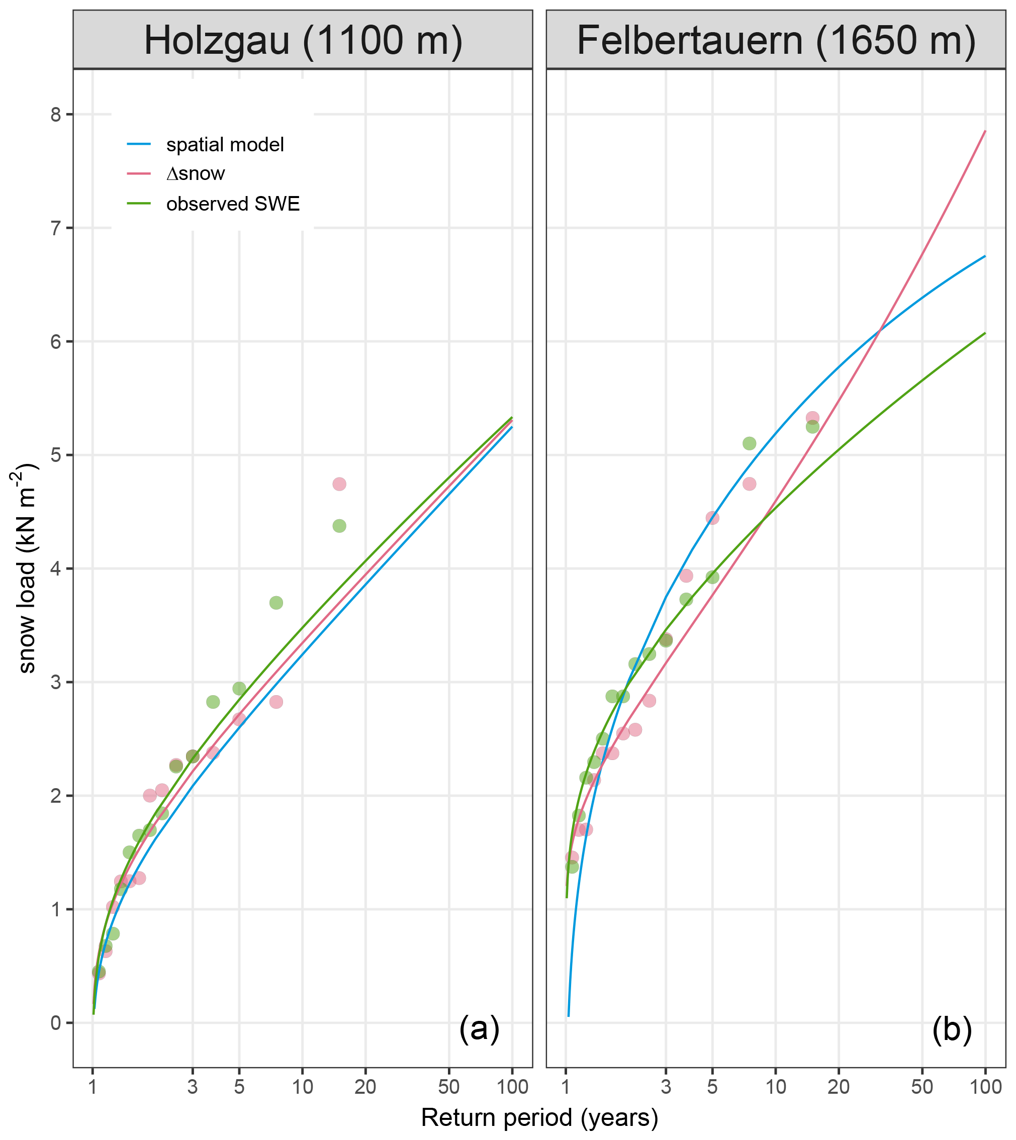
Figure C2Return levels of snow load at stations Holzgau (left) and Felbertauern (right). Return periods in years are shown on the logarithmic x axis. The blue line shows return levels obtained with the spatial extreme value model, pink bullets and lines depict yearly maxima and the GEV fit of SWE values modeled from daily snow depths with the Δsnow model, and green colors represent yearly SWE maxima and the corresponding GEV fit from (ca. weekly) observations.
R code of Δsnow and some empirical regression models: https://cran.r-project.org/package=nixmass (last access: 2 March 2021) (Schellander, 2020). Phyton code of Δsnow, ported by Manuel Theurl (Graz University of Technology, Austria): https://bitbucket.org/atraxoo/snow_to_swe (last access: 2 March 2021) (Theurl, 2020).
MW started and led the project and structured and managed it. He was a key figure in developing and designing the snow model, and he did most of the writing. HS developed, coded, and calibrated the model. He wrote the R package and helped with writing the paper, particularly the application example in the Appendix. SG developed early versions of the model and its code.
The authors declare that they have no conflict of interest.
The authors want to acknowledge Tobias Hell (Department of Mathematics, University of Innsbruck, Austria), who substantially helped with the Scaling module (Sect. 2.3.2 and Appendix B). Thanks also go to the Hydrographic Service of Tyrol (Austria), which provided part of the data. Alexander Radlherr and Jutta Staudacher (ZAMG, Austria) are thanked for vivid discussions and early proofreading; special thanks are given to Lindsey Nicholson (University of Innsbruck, Austria) for final proofreading. Not least, we want to acknowledge Manuel Theurl (Graz University of Technology, Austria) and Jakob Abermann (University of Graz, Austria) for porting Δsnow's R code to Phyton. The authors highly appreciate the comments and suggestions of the editor and the three anonymous referees. They significantly improved the article.
This work was embedded in the project “Schneelast.Reform”, funded by the Austrian Research Promotion Agency (FFG) and the Austrian Economic Chamber (WKO), in particular by their Association of the Austrian Wood Industries (FV Holzindustrie).
This paper was edited by Markus Weiler and reviewed by three anonymous referees.
Akaike, H.: A new look at the statistical model identification, IEEE T. Automat. Control, 19, 716–723, https://doi.org/10.1109/TAC.1974.1100705, 1974. a
Armstrong, R. L. and Brun, E.: Snow and climate: physical processes, surface energy exchange and modeling, Cambridge University Press, Cambridge, 2010. a
Austrian Standards Institute: ÖNORM B 1991-1-3:2018-12-01, Vienna, Austria, 2018. a, b, c
Avanzi, F., De Michele, C., and Ghezzi, A.: On the performances of empirical regressions for the estimation of bulk snow density, Geografia Fisica e Dinamica Quaternaria, 38, 105–112, https://doi.org/10.4461/GFDQ.2015.38.10, 2015. a, b, c, d
Blanchet, J. and Davison, A.: Spatial modeling of extreme snow depth, Ann. Appl. Stat., 5, 1699–1725, https://doi.org/10.1214/11-AOAS464SUPP, 2011. a
Blanchet, J. and Lehning, M.: Mapping snow depth return levels: smooth spatial modeling versus station interpolation, Hydrol. Earth Syst. Sci., 14, 2527–2544, https://doi.org/10.5194/hess-14-2527-2010, 2010. a, b
Byrd, R. H., Lu, P., Nocedal, J., and Zhu, C.: A Limited Memory Algorithm for Bound Constrained Optimization, SIAM J. Scient. Comput., 16 1190–1208, https://doi.org/10.1137/0916069, 1995. a
Coles, S.: An introduction to statistical modeling of extreme values, in: Springer Series in Statistics, Springer-Verlag, London, 2001. a
Cuffey, K. and Paterson, W. S. B.: The physics of glaciers, 4th Edn., oCLC: ocn488732494, Butterworth-Heinemann/Elsevier, Burlington, MA, 2010. a, b, c
Deems, J. S., Painter, T. H., and Finnegan, D. C.: Lidar measurement of snow depth: a review, J. Glaciol., 59, 467–479, https://doi.org/10.3189/2013JoG12J154, 2013. a
De Michele, C., Avanzi, F., Ghezzi, A., and Jommi, C.: Investigating the dynamics of bulk snow density in dry and wet conditions using a one-dimensional model, The Cryosphere, 7, 433–444, https://doi.org/10.5194/tc-7-433-2013, 2013. a, b, c
Denoth, A.: The Pendular-Funicular Liquid Transition and Snow Metamorphism, J. Glaciol., 28, 357–364, https://doi.org/10.3189/S0022143000011692, 1982. a
Dietz, A., Kuenzer, C., Gessner, U., and Dech, S.: Remote Sensing of Snow – a Review of available methods, Int. J. Remote Sens., 33, 4094–4134, https://doi.org/10.1080/01431161.2011.640964, 2012. a
Dixon, D. and Boon, S.: Comparison of the SnowHydro snow sampler with existing snow tube designs, Hydrol. Process., 26, 2555–2562, https://doi.org/10.1002/hyp.9317, 2012. a
Egli, L., Jonas, T., and Meister, R.: Comparison of different automatic methods for estimating snow water equivalent, Cold Reg. Sci. Technol., 57, 107–115, https://doi.org/10.1016/j.coldregions.2009.02.008, 2009. a, b
eHORA: Natural Hazard Overview & Risk Assessment Austria, available at: https://hora.gv.at/ (last access: 6 January 2021), 2006. a
Essery, R., Morin, S., Lejeune, Y., and Ménard, C. B.: A comparison of 1701 snow models using observations from an alpine site, Adv. Water Resour., 55, 131–148, https://doi.org/10.1016/j.advwatres.2012.07.013, 2013. a, b, c
European Committee for Standardization: EN 1991-1-3:2003/A1:2015, Brussels, Belgium, 2015. a
Fierz, C., Armstrong, R., Durand, Y., Etchevers, P., Greene, E., McClung, D., Nishimura, K., Satyawali, P., and Sokratov, S.: The International Classification for Seasonal Snow on the Ground, IHP-VII Technical Documents in Hydrology, 83 pp., available at: http://unesdoc.unesco.org/images/0018/001864/186462e.pdf (last access: 2 March 2021), 2009. a
Garvelmann, J., Pohl, S., and Weiler, M.: From observation to the quantification of snow processes with a time-lapse camera network, Hydrol. Earth Syst. Sci., 17, 1415–1429, https://doi.org/10.5194/hess-17-1415-2013, 2013. a
Goodison, B. E., Ferguson, H. L., and McKay, G. A.: Measurement and data analysis, in: Handbook of Snow: Principles, Processes, Management and Use, edited by Gray, D. M. and Male, D. H., Pergamon Press, Toronto, Canada, 191–274, 1981. a, b
Gruber, S.: Modelling snow water equivalent based on daily snow depths, MS thesis, University of Innsbruck, Innsruck, 2014. a, b, c, d, e, f, g
Guyennon, N., Valt, M., Salerno, F., Petrangeli, A. B., and Romano, E.: Estimating the snow water equivalent from snow depth measurements in the Italian Alps, Cold Reg. Sci. Technol., 167, 102859, https://doi.org/10.1016/j.coldregions.2019.102859, 2019. a, b, c, d, e, f, g, h, i
Haberkorn, A.: European Snow Booklet – an Inventory of Snow Measurements in Europe, EnviDat, https://doi.org/10.16904/envidat.59, 2019. a
Heilig, A., Schneebeli, M., and Eisen, O.: Upward-looking ground-penetrating radar for monitoring snowpack stratigraphy, Cold Reg. Sci. Technol., 59, 152–162, https://doi.org/10.1016/j.coldregions.2009.07.008, 2009. a
Helfricht, K., Hartl, L., Koch, R., Marty, C., and Olefs, M.: Obtaining sub-daily new snow density from automated measurements in high mountain regions, Hydrol. Earth Syst. Sci., 22, 2655–2668, https://doi.org/10.5194/hess-22-2655-2018, 2018. a, b, c, d
Hill, D. F., Burakowski, E. A., Crumley, R. L., Keon, J., Hu, J. M., Arendt, A. A., Wikstrom Jones, K., and Wolken, G. J.: Converting snow depth to snow water equivalent using climatological variables, The Cryosphere, 13, 1767–1784, https://doi.org/10.5194/tc-13-1767-2019, 2019. a
Johnson, J. B., Gelvin, A. B., Duvoy, P., Schaefer, G. L., Poole, G., and Horton, G. D.: Performance characteristics of a new electronic snow water equivalent sensor in different climates, Hydrol. Process., 29, 1418–1433, https://doi.org/10.1002/hyp.10211, 2015. a
Jonas, T., Marty, C., and Magnusson, J.: Estimating the snow water equivalent from snow depth measurements in the Swiss Alps, J. Hydrol., 378, 161–167, https://doi.org/10.1016/j.jhydrol.2009.09.021, 2009. a, b, c, d, e, f, g, h, i, j, k, l, m, n, o, p, q
Jordan, R.: A One-Dimensional Temperature Model for a Snow Cover: Technical documentation for SNTHERM.89, Tech. rep., Corps of Engineers, US Army Cold Regions Research & Engineering Laboratory, Hanover, New Hampshire, USA, 1991. a, b, c
Jordan, R., Albert, M., and Brun, E.: Physical Processes within the snow cover and their parametrization, in: Snow and Climate: Physical Processes, Surface Energy Exchange and Modeling, Cambridge University Press, Cambridge, 12–69, 2010. a, b, c, d, e, f, g
Keeler, C.: Some Physical Properties of Alpine Snow, Tech. rep., Corps of Engineers, US Army Cold Regions Research & Engineering Laboratory, Hanover, New Hampshire, USA, 1969. a, b
Kinar, N. J. and Pomeroy, J. W.: Measurement of the physical properties of the snowpack, Rev. Geophys., 53, 481–544, https://doi.org/10.1002/2015RG000481, 2015. a, b, c, d
Koch, F., Henkel, P., Appel, F., Schmid, L., Bach, H., Lamm, M., Prasch, M., Schweizer, J., and Mauser, W.: Retrieval of Snow Water Equivalent, Liquid Water Content, and Snow Height of Dry and Wet Snow by Combining GPS Signal Attenuation and Time Delay, Water Resour. Res., 55, 4465–4487, https://doi.org/10.1029/2018WR024431, 2019. a
Kojima, K.: Densification of Seasonal Snow Cover, in: Physics of Snow and Ice: proceedings, vol. 1 of 2, Sapporo, Japan, 929–952, available at: http://hdl.handle.net/2115/20351 (last access: 2 March 2021), 1967. a
Langlois, A., Kohn, J., Royer, A., Cliche, P., Brucker, L., Picard, G., Fily, M., Derksen, C., and Willemet, J. M.: Simulation of Snow Water Equivalent (SWE) Using Thermodynamic Snow Models in Québec, Canada, J. Hydrometeorol, 10, 1447–1463, https://doi.org/10.1175/2009JHM1154.1, 2009. a, b, c
Lehning, M., Bartelt, P., Brown, R., Fierz, C., and Satyawali, P.: A physical SNOWPACK model for the Swiss Avalanche Warning Services. Part II: Snow Microstructure, Cold Reg. Sci. Technol., 35, 147–167, 2002. a
Leppänen, L., Kontu, A., and Pulliainen, J.: Automated Measurements of Snow on the Ground in Sodankylä, Geophysica, 53, 45–64, 2018. a
Lievens, H., Demuzere, M., Marshall, H.-P., Reichle, R. H., Brucker, L., Brangers, I., de Rosnay, P., Dumont, M., Girotto, M., Immerzeel, W. W., Jonas, T., Kim, E. J., Koch, I., Marty, C., Saloranta, T., Schöber, J., and De Lannoy, G. J. M.: Snow depth variability in the Northern Hemisphere mountains observed from space, Nat. Commun., 10, 4629, https://doi.org/10.1038/s41467-019-12566-y, 2019. a
López-Moreno, J. I., Leppänen, L., Luks, B., Holko, L., Picard, G., Sanmiguel-Vallelado, A., Alonso-González, E., Finger, D. C., Arslan, A. N., Gillemot, K., Sensoy, A., Sorman, A., Ertaş, M. C., Fassnacht, S. R., Fierz, C., and Marty, C.: Intercomparison of measurements of bulk snow density and water equivalent of snow cover with snow core samplers: Instrumental bias and variability induced by observers, Hydrol. Process., 34, 3120–3133, https://doi.org/10.1002/hyp.13785, 2020. a, b
Mair, E., Leitinger, G., Della Chiesa, S., Niedrist, G., Tappeiner, U., and Bertoldi, G.: A simple method to combine snow height and meteorological observations to estimate winter precipitation at sub-daily resolution, Hydrolog. Sci. J., 61, 2050–2060, https://doi.org/10.1080/02626667.2015.1081203, 2016. a
Marks, D. G., Kimball, J. S., Tingey, D., and Link, T. E.: The Sensitivity of Snowmelt Processes to Climate Conditions and Forest Cover during Rain-on-Snow: A Case Study of the 1996 Pacific Northwest Flood, Hydrol. Process., 12, 1569–1587, 1998. a
Martinec, J.: Zimni prognosy s pouzitim radioisotopu (Winter forecasts with the use of radioisotopes), Vltavska kaskada (The Vltava reservoir system), VUV Praha-Podbab, Praha, Czech Republic, 45–60, 1956. a
Martinec, J.: Expected snow loads on structures from incomplete hydrological data, J. Glaciol., 19, 185–195, https://doi.org/10.3189/S0022143000029270, 1977. a, b, c
Martinec, J. and Rango, A.: Indirect evaluation of snow reserves in mountain basins, in: Proceedings of the Vienna Symposium, August 1991, Vienna, IAHS – International Association of Hydrological Sciences, 111–120, available at: http://hydrologie.org/redbooks/a205/iahs_205_0111.pd (last access: 2 March 2021) 1991. a, b, c, d, e, f, g, h
Marty, C.: GCOS SWE data from 11 stations in Switzerland, type: dataset, https://doi.org/10.16904/15, 2017. a, b, c
McCreight, J. L. and Small, E. E.: Modeling bulk density and snow water equivalent using daily snow depth observations, The Cryosphere, 8, 521–536, https://doi.org/10.5194/tc-8-521-2014, 2014. a, b, c, d
Mitterer, C., Hirashima, H., and Schweizer, J.: Wet-snow instabilities: comparison of measured and modelled liquid water content and snow stratigraphy, Ann. Glaciol., 52, 201–208, https://doi.org/10.3189/172756411797252077, 2011. a
Mizukami, N. and Perica, S.: Spatiotemporal Characteristics of Snowpack Density in the Mountainous Regions of the Western United States, J. Hydrometeorol., 9, 1416–1426, https://doi.org/10.1175/2008JHM981.1, 2008. a, b, c
Nash, J. C.: On Best Practice Optimization Methods in R, J. Stat. Softw., 60, 1–14, 2014. a
Olefs, M., Schöner, W., Suklitsch, M., Wittmann, C., Niedermoser, B., Neururer, A., and Wurzer, A.: SNOWGRID – A New Operational Snow Cover Model in Austria, in: International Snow Science Workshop, 7–11 October 2013, Grenoble, Chamonix Mont-Blanc, 38–45, available at: https://arc.lib.montana.edu/snow-science/item/1785 (last access: 2 March 2021), 2013. a
Painter, T. H., Berisford, D. F., Boardman, J. W., Bormann, K. J., Deems, J. S., Gehrke, F., Hedrick, A., Joyce, M., Laidlaw, R., Marks, D., Mattmann, C., McGurk, B., Ramirez, P., Richardson, M., Skiles, S. M., Seidel, F. C., and Winstral, A.: The Airborne Snow Observatory: Fusion of scanning lidar, imaging spectrometer, and physically-based modeling for mapping snow water equivalent and snow albedo, Remote Sens. Environ., 184, 139–152, https://doi.org/10.1016/j.rse.2016.06.018, 2016. a
Parajka, J., Haas, P., Kirnbauer, R., Jansa, J., and Blöschl, G.: Potential of time-lapse photography of snow for hydrological purposes at the small catchment scale, Hydrol. Process., 26, 3327–3337, https://doi.org/10.1002/hyp.8389, 2012. a
Pistocchi, A.: Simple estimation of snow density in an Alpine region, J. Hydrol.: Reg. Stud., 6, 82–89, https://doi.org/10.1016/j.ejrh.2016.03.004, 2016. a, b, c, d, e, f
Powell, M.: The BOBYQA algorithm for bound constrained optimization without derivatives, Report DAMTP 2009/NA06, University of Cambridge, Cambridge, availalbe at: https://www.damtp.cam.ac.uk/user/na/NA_papers/NA2009_06.pdf (last access: 2 March 2021), 2009. a
R Core Team: R: A Language and Environment for Statistical Computing, R Foundation for Statistical Computing, Vienna, Austria, available at: https://www.R-project.org/ (last access: 2 March 2021), 2019. a, b
Rohrer, M. and Braun, L.: Long-Term Records of Snow Cover Water Equivalent in the Swiss Alps, Nord. Hydrol., 25, 65–78, https://doi.org/10.2166/nh.1994.0020, 1994. a, b, c, d, e
Sandells, M., Flerchinger, G. N., Gurney, R., and Marks, D. G.: Simulation of snow and soil water content as a basis for satellite retrievals, Hydrol. Res., 43, 720–735, https://doi.org/10.2166/nh.2012.028, 2012. a, b, c
Schattan, P., Köhli, M., Schrön, M., Baroni, G., and Oswald, S. E.: Sensing Area-Average Snow Water Equivalent with Cosmic-Ray Neutrons: The Influence of Fractional Snow Cover, Water Resour. Res., 55, 10796–10812, https://doi.org/10.1029/2019WR025647, 2019. a
Schellander, H.: nixmass: Snow Water Equivalent Modeling with the `Delta.snow' Model and Empirical Regression Models, R package version 1.0-1, available at: https://CRAN.R-project.org/package=nixmass (last access: 2 March 2021), 2020. a
Schellander, H. and Hell, T.: Modeling snow depth extremes in Austria, Nat. Hazards, 94, 1367–1389, https://doi.org/10.1007/s11069-018-3481-y, 2018. a
Seibert, P., Frank, A., and Formayer, H.: Synoptic and regional patterns of heavy precipitation in Austria, Theor. Appl. Climatol., 87, 139–153, https://doi.org/10.1007/s00704-006-0198-8, 2007. a
Smith, C. D., Kontu, A., Laffin, R., and Pomeroy, J. W.: An assessment of two automated snow water equivalent instruments during the WMO Solid Precipitation Intercomparison Experiment, The Cryosphere, 11, 101–116, https://doi.org/10.5194/tc-11-101-2017, 2017. a, b
Smyth, E. J., Raleigh, M. S., and Small, E. E.: Particle Filter Data Assimilation of Monthly Snow Depth Observations Improves Estimation of Snow Density and SWE, Water Resour. Res., 55, 1296–1311, https://doi.org/10.1029/2018WR023400, 2019. a, b, c
Sturm, M. and Holmgren, J.: Differences in compaction behavior of three climate classes of snow, Ann. Glaciol., 26, 125–130, 1998. a, b, c, d, e, f, g, h, i, j, k
Sturm, M., Taras, B., Liston, G. E., Derksen, C., Jonas, T., and Lea, J.: Estimating Snow Water Equivalent Using Snow Depth Data and Climate Classes, J. Hydrometeorol., 11, 1380–1394, https://doi.org/10.1175/2010JHM1202.1, 2010. a, b, c, d, e, f, g, h, i, j, k, l, m, n
Theurl, M.: snow_to_swe, available at: https://bitbucket.org/atraxoo/snow_to_swe (last access: 2 March 2021), 2020. a
Valt, M., Romano, E., and Guyennon, N.: Snowcover density and snow water equivalent in the Italian Alps, in: Proceedings ISSW 2018, International Snow Science Workshop, Innsbruck, Austria, 2018. a
Vionnet, V., Brun, E., Morin, S., Boone, A., Faroux, S., Le Moigne, P., Martin, E., and Willemet, J. M.: The detailed snowpack scheme Crocus and its implementation in SURFEX v7.2, Geosci. Model Dev., 5, 773–791, https://doi.org/10.5194/gmd-5-773-2012, 2012. a, b, c, d, e, f
Wastl, C.: Klimatologische Analyse von orographisch beeinflussten Niederschlagsstrukturen im Alpenraum, PhD thesis, Ludwig-Maximilians-Universität München, München, https://doi.org/10.5282/edoc.9545, 2008. a
Wever, N., Schmid, L., Heilig, A., Eisen, O., Fierz, C., and Lehning, M.: Verification of the multi-layer SNOWPACK model with different water transport schemes, The Cryosphere, 9, 2271–2293, https://doi.org/10.5194/tc-9-2271-2015, 2015. a, b
ΔSNOW model, its code is freely available, and it can be applied in various climates. The method is especially interesting for studies on extremes (e.g., snow loads or flooding) and climate (e.g., precipitation trends).