the Creative Commons Attribution 4.0 License.
the Creative Commons Attribution 4.0 License.
 | 05 Mar 2021
Partial energy balance closure of eddy covariance evaporation measurements using concurrent lysimeter observations over grassland
Peter Widmoser
Dominik Michel
With respect to ongoing discussions about the causes of energy imbalance and approaches to force energy balance closure, a method has been proposed that allows partial latent heat flux closure (Widmoser and Wohlfahrt, 2018). In the present paper, this method is applied to four measurement stations over grassland under humid and semiarid climates, where lysimeter (LY) and eddy covariance (EC) measurements were taken simultaneously.
The results differ significantly from the ones reported in the literature. We distinguish between the resulting EC values being weakly and strongly correlated to LY observations as well as systematic and random deviations between the LY and EC values. Overall, an excellent match could be achieved between the LY and EC measurements after applying evaporation-linked weights. But there remain large differences between the standard deviations of the LY and adjusted EC values. For further studies we recommend data collected at time intervals even below 0.5 h.
No correlation could be found between evaporation weights and weather indices. Only for some datasets, a positive correlation between evaporation and the evaporation weight could be found. This effect appears pronounced for cases with high radiation and plant water stress.
Without further knowledge of the causes of energy imbalance one might perform full closure using equally distributed weights. Full closure, however, is not dealt with in this paper.
- Article
(2651 KB) - Full-text XML
- BibTeX
- EndNote


Non-closure of the surface energy balance, i.e., the sum of latent (LE) and sensible (H) heat exchange falling short of available energy (A), is a common issue in eddy covariance flux (EC) measurements. Available energy equals net radiation (RN) minus the soil heat flux (G) and any other energy storage (Wohlfahrt and Widmoser, 2013). At the majority of eddy covariance flux sites, it is the rule rather than the exception to find that the sum of the turbulent fluxes LE+H underestimates A by 20 %–30 % (Leuning et al., 2012; Wilson et al., 2002). This apparently systematic bias has been extensively discussed in the literature (see reviews by Foken, 2008; Foken et al., 2011; Leuning et al., 2012; Mauder et al., 2020). In the most recent review, the following classification of reasons for the energy gap problem is listed: (1) instrument error, (2) data processing error, (3) additional sources of energy and (4) secondary circulation of energy. Our own hourly observations show that the bulk of LE+H underestimates is detected around noon, whereas during sunrise and sunset overestimates are also observed.
There are two practical approaches to deal with the energy imbalance problem: (1) comparing EC measurements with concurrent lysimeter measurements and (2) using models.
Lysimeters (LY) have a long tradition in hydrology and micrometeorology, and their limitations and sources of uncertainty are well known. There usually is a very strong correlation between concurrent LY- and EC-based evaporation data, with the LY values generally being higher. An overview of efforts to compare EC evaporation to lysimeter measurements can be found in Gebler et al. (2015). A few of the studies related to this article are described below.
Chavez and Howell (2009) hint at various error sources for the LY and EC measurements. EC observations on cotton fields in Texas with quarter-hourly measurements resulted in an energy balance gap of 22.0 % to 26.8 %. Those gaps were closed assuming Bowen ratio preservation and correct measurements of the available energy. After forced closure of the energy balance, the difference between daytime LY and EC data on two fields could be reduced from −28.8 % to 6.2 % and from −26.0 % to −12.3 %, respectively, with an accuracy of 0.03±0.5 mm d−1 () and mm d−1 (), respectively. Negative values indicate that the lysimeter values were higher on average than the EC values.
Evett et al. (2012), using data from the same site as Chavez and Howell (2009), report errors of daytime EC measurements for latent heat flux of 1.9 to 2.7 mm d−1 (≈55 to 78 W m−2) and for sensible heat flux of 1.4 to 1.9 mm d−1 (≈40 to 55 W m−2). They reported substantially larger LY evaporation rates compared to the EC measurements due to differences in plant growth in the LY and the EC footprint. After forced closure of the energy gap, as done by Chavez and Howell (2009), mean differences from −17.4 % to −18.7 % were found between the two measurement methods after correcting for plant growth.
In the same way, Ding et al. (2010) closed the energy gaps using half-hourly daytime data on irrigated maize in an arid area in northwest China. Differences in daily measurements were also reduced there by forced Bowen ratio closure of the EC gap. Differences could be reduced from −22.4 % to −6.2 %, with the lysimeter measurements again being higher on average.
The following authors dealt with comparing measurements on grassland. Gebler et al. (2015) assumed that the energy balance deficit is only caused by an underestimation of the turbulent fluxes, which are corrected according to the evaporative fraction averaged over 7 d. After correction, they find an agreement between the LY and EC values with a total difference of 3.8 % (19 mm) over a year. The best agreements on the basis of monthly values during summer were obtained with less than 8 % relative errors. The remaining differences are suspected to be due to different plant height within the EC fetch and the lysimeter. Mauder et al. (2018) evaluated two adjustment methods to close the energy balance: (1) the Bowen ratio preservation adjustment, following the approach of Mauder et al. (2013) and (2) the method by Charuchittipan et al. (2014), which attributes a larger portion of the residual to the sensible heat flux. They also compare the EC values with the results of the hydrological model GEOtop 2.0 (Endrizzi et al., 2014). They found that a daily adjustment factor leads to less scatter than a complete partitioning of the residual for every 0.5 h time interval.
In the compilation of the literature above, the LY–EC comparisons relied on the assumptions that the available energy observations are correct and that the Bowen ratio can be preserved. In contrast to the closure method used by the abovementioned authors, Widmoser and Wohlfahrt (2018) achieved a partial latent heat closure of the energy balance by combining both the model and lysimeter approach, which is afterwards fully closed under the assumption of preservation of the Bowen ratio.
The objective of this article is to extend the abovementioned method, which was applied to only one station, to more stations in order to test its applicability and compare its results.
2.1 Measurement stations and data sets
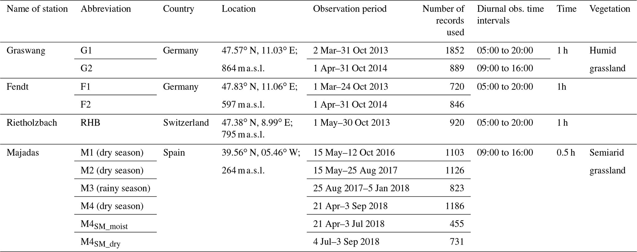
Table 1 specifies the stations from which data were used.
Table 1Specifications of data used; SM denotes soil moisture.
Data were obtained from the following institutions: (1) Graswang (G) and Fendt (F) from M. Mauder, Institute of Technology (KIT-Karlsruhe), Garmisch-Partenkirchen, Germany; and R. Kiese, Institute for Technology, Institute of Meteorology and Climate, Karlsruhe, Germany; (2) Majadas (M) from M. Migliavacca and O. Perez-Priego, Max Planck Institute for Biogeochemistry, Jena, Germany; and (3) Rietholzbach (RHB) from S. I. Seneviratne and M. Hirschi, Institute for Atmospheric and Climate Science, ETH Zurich, Switzerland.
2.1.1 Graswang and Fendt
The Graswang and Fendt stations are both located in grassland ecosystems mostly used for fodder and hay production in the Ammer catchment area in the south of Germany. These sites belong to the Bavarian Alps/pre-Alps observatory of the TERrestrial Environmental Observatories (TERENO) network (Zacharias et al., 2011) and are part of the Integrated Carbon Observation System (ICOS, https://icos-infrastruktur.de, last access: 22 February 2021). The soil in Fendt is classified as cambic Stagnosol and the mean annual precipitation and temperature in 2013 and 2014 were 922 mm and 8.7 ∘C, respectively. The soil in Graswang is classified as fluvic calcaric Cambisol and the mean annual precipitation and temperature in 2013 and 2014 were 1238 mm and 6.7 ∘C, respectively. In both cases the site management at the EC tower and on the lysimeters followed the farmers' practices. The practice in Fendt was extensive (two cuts and two manure applications), while it was intensive in Graswang (five cuts and four manure applications; Mauder et al., 2018).
The equipment used in this study is identical for both stations. EC instrumentation comprises a CSAT-3 sonic anemometer (Campbell Scientific Inc. USA) and an LI-7500 infrared gas analyzer (LI-COR Biosciences, USA) at 2 . Available energy (W m−2) was observed using a CNR4 net radiometer (Kipp & Zonen, The Netherlands) at 2 and the average of three HFP01-SC heat flux plates (Hukseflux, The Netherlands) at a depth of 0.08 m. Spatially averaged soil moisture data (m3 m−3) were obtained with three CS616 soil moisture sensors (Campbell Scientific Inc. USA) at a depth of 0.06 m. Lysimeter evaporation (W m−2) was obtained with a lower boundary-controlled TERENO-SOILCan large weighing lysimeter (METER Group AG, Germany; described by Gebler et al., 2015 and Mauder et al., 2018) with a surface area of 1.0 m2 and a depth of 1.5 m. The temporal resolution of all data from these stations is 1 h.
2.1.2 Rietholzbach
The Rietholzbach hydrometeorological research station is located in northeastern Switzerland in a hilly, pre-alpine catchment draining an area of 3.31 km2. The region is characterized by a temperate humid climate with a mean annual precipitation and air temperature of 1438 mm and 7.1 ∘C, respectively, based on the 1976–2015 long-term mean. The soil type and depth exhibit a high spatial variability. Overall, shallow Regosols dominate on steep slopes, deeper Cambisols are found in flatter areas and gley soils are located in the vicinity of small creeks. On the slopes and along creeks, in about 25 % of the area, forest dominates. The remaining catchment area is mostly grassland and partially used as pasture (Hirschi et al., 2017).
EC fluxes were measured with a CSAT3 sonic anemometer (Campbell Scientific Inc. USA) and an LI-7500 infrared gas analyzer (LI-COR Biosciences, USA) at 2 . Net radiation was measured using two CM21 pyranometers (Kipp & Zonen, The Netherlands) for the net shortwave radiation and two CG4 net radiometers (Kipp & Zonen, The Netherlands) for the net longwave radiation, both at 2 . The soil heat flux was calculated as the average of three HFP01 and one HFP01-SC heat flux plates (Hukseflux, The Netherlands) at a depth of 0.05 m. The Rietholzbach large weighing lysimeter has a surface area of 3.1 m2 and a depth of 2.5 m including a gravel filter layer at the bottom and gravitational discharge. The temporal resolution of all data from this station is 1 h. For more information on this station refer to Seneviratne et al. (2012) and Hirschi et al. (2017).
2.1.3 Majadas
The Majadas del Tiétar North station is located in a Mediterranean tree-grass savannah in western Spain. It is part of the FLUXNET network (fluxnet.ornl.gov). The vegetation cover is composed of trees (mostly Quercus ilex (L.), approx. 22 trees ha−1) and an herbaceous stratum composed of native annual species of the three main functional plant forms (grasses, forbs and legumes). The soil is classified as an Abruptic Luvisol and the mean annual precipitation and temperature are 650 mm and 16 ∘C, respectively (Perez-Priego et al., 2017).
EC fluxes are obtained with a Gill R3-50 sonic anemometer (Gill Instruments Ltd., UK) and an LI-7200 infrared gas analyzer (LI-COR Biosciences, USA) at 15.5 . Available energy was observed using a CNR4 net radiometer (Kipp & Zonen, The Netherlands) and the average of four HFP01-SC heat flux plates (Hukseflux, The Netherlands) at a depth of 0.03 m. Spatially averaged soil moisture data were obtained with two Enviroscan soil moisture sensors (Sentek, Australia) at a depth of 0.40 m. Lysimeter evaporation data are the spatial average of four lower boundary-controlled large weighing lysimeters (Umwelt-Geräte-Technik GmbH, Germany) with a surface area of 1.0 m2 and a depth of 1.2 m. The used temporal resolution of all data from this station is 0.5 h. For more information on the station refer to Migliavacca et al. (2017) and Perez-Priego et al. (2017).
Figure 1 and Table 1 give an overview of the locations of the stations and time periods used. Note that for G1, F1, F2 and RHB, measurements between 05:00 and 20:00 were used. The times of day used for G2 and Majadas were reduced to 09:00 to 16:00 for the reasons given below (Sect. 2.4). Figure 2 shows the mean daytime course of A, H, LY- and EC-based LE as well as the resulting energy gap, ε, at all four stations.
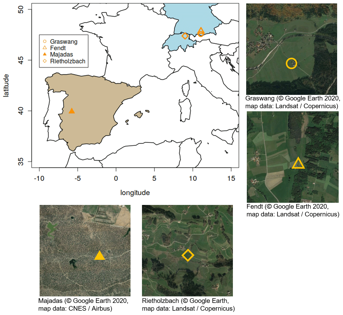
Figure 1Location and satellite view of the stations used and their surrounding area. The symbols denote the locations of the lysimeters.
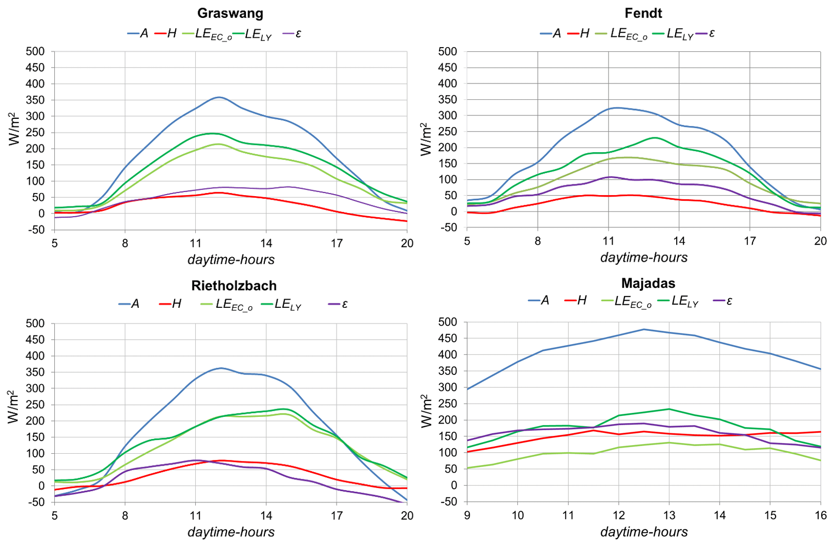
Figure 2Average daytime course of available energy (A), sensible heat flux (H), EC-based (LEEC_o) and lysimeter-based (LELY) latent heat flux and the energy gap (ε) at the four stations. Note that for Majadas the diurnal cycle represents the dry season (M4).
2.2 Possible errors of lysimeter observations
The lysimeters used in this study can achieve measurement accuracies equivalent to between ±7 and , depending on their construction. Furthermore, hydraulic conditions (cylinder walls, soil conditions and ground water table) of the lysimeter do not correspond with the undisturbed surrounding. In addition to these systematic errors, random errors may occur due to instabilities caused by wind gusts. One may also note that lysimeter observations generally do not include negative values (condensation). The influence of wind and dew on lysimeter observations is described in Meissner et al. (2007) and Ruth et al. (2018). The theoretical accuracy of lysimeter measurements can be calculated from the surface area and weighing accuracy. For the RHB lysimeter (operational since 1976), a systematic accuracy of about 0.03 mm (equivalent to approx. within an hourly interval) is reported by Hirschi et al. (2017). All other lysimeters of this study (in F, G and M) have a calculated systematic accuracy of 0.01 mm (equivalent to approx. within an hourly interval).
2.3 Possible errors of the EC observations
Systematic measuring errors of the latent heat flux (LE) may be around of sensible heat flux (H) around ±13 W m−2 and of available radiation around (Alfieri et al., 2012).
Errors caused by non-closure of the energy balance are not included in the estimates given above. The ε errors result as the sum of A, LE and H errors and may be around .
2.4 Data selection
High quality data were available from all the observation stations. Still we had to dismiss 2 % to 5 % of the EC measurements, mostly for morning and evening hours with high instability of turbulent fluxes. We sorted them out on the basis of the out-of-bound concept introduced by Wohlfahrt and Widmoser (2013), which excludes physically unrealistic measurements. According to this concept, the ratio , where ra and rc denote aerodynamic and canopy resistance, must numerically be within the range of 1 to infinity (see Fig. 1 in Wohlfahrt and Widmoser, 2013). Case 2 represents r1<0 and case 3 represents . Data corresponding to case 2 and 3 are thus omitted. Furthermore, data showing big differences between the LY and EC measurements (i.e., ) along with strong wind gusts (), as well as early morning values with high air humidity and high dew formation were also excluded, thus reducing the original data sets by another 5 % on average.
The overall data selection led to a reduced number of early morning and late evening data as compared to the number of records available for the rest of the day. This means that results around sunrise and sunset are generally less reliable. In the case of G2, the morning and evening data had to be reduced to such an extent that we decided to only evaluate data from 09:00 to 16:00. For Majadas, all morning data were omitted for this reason. The numbers of records used given in Table 1 correspond to the data analyzed below.
In order to extend the daily time window of analyzed Majadas data (i.e., from 05:00 to 20:00) in the M4 dataset (dry season), the morning and evening values were corrected for dew effects. In this way, we obtained wLE estimates (wLE_long is ca. 0.4, see Fig. 8b), which compare well with the results of the other stations.
2.5 Evaluation of weights wLE by regression (partial closure)
Wohlfahrt and Widmoser (2013) introduced a simple framework for studying the energy imbalance (ε), i.e.,
They proposed three dimensionless weights (wA, wH and wLE) for the terms on the RHS of Eq. (1), which obey the following two constraints: (i) each weight is bound between zero and unity and (ii) the three weights sum up to unity.
Provided these weights are known, the terms on the RHS of Eq. (1) can be corrected for the lack of energy balance closure as
In this paper, we are concerned only with the evaluation of wLE (Eq. 2c) by regressing the difference between the LY and EC latent heat fluxes as a function of the energy imbalance:
where LELY and LEEC denote the latent heat flux from the LY and EC measurements, respectively, wLE represents the slope of the best-fit linear relationship and the y-intercept (d) might be interpreted as a systematic difference between the LY and EC latent heat flux measurements. The random difference follows from
For regression, data were binned according to the magnitude of LE in such a way that for each bin the same number of data pairs (LY–EC) vs. ε, see Eq. (3), was available. The number of records, i.e., 5 to 14, depended on the number of data per dataset available. At least 90 data pairs entered each regression.
2.6 Used parameters
The results of the partial energy closure will be represented by the following parameters:
-
as the difference between the observed LY and observed LEEC_o values
-
as the difference between the observed LY and corrected LEEC_c values:
-
as the difference between the observed LY and adjusted LEEC_a values: .
Furthermore we list the
-
systematic deviations, d, see the intercept in Eq. (3)
-
as a measure for the relative ε remaining after adjustment; εred=ε (1−wLE)
-
weight wLE.
One may note that the Da values correspond to the remaining differences after LEEC adjustment to the LY data and as such may be interpreted as random deviations drand or noise.
3.1 Basic evaporation characteristics
Table 2a and b gives means and standard deviations (SDs) of the observed LEEC_o, the corrected LEEC_c, the adjusted LEEC_a and LY evaporations for the analyzed periods and stations along with energy balance deficit ε, and correlation coefficients between the LY and EC data. They highlight the substantial difference between the humid and dry stations in terms of the mean magnitude of evaporation. Under moist soil conditions (M4), in contrast, the dry station Majadas ranges around the same magnitude as the humid stations.
Table 2(a) Basic evaporation characteristics for the humid stations (ρ= correlation coefficient). (b) Basic evaporation characteristics for the Majadas stations (ρ= correlation coefficient).

One may note that F1 has the lowest evaporation rate among the humid stations. This will influence the following results throughout.
3.2 Differences between means and standard deviations of the LY and EC measurements
Table 3a and b shows the absolute differences and their standard deviation between the EC data presented in Table 2a and b and the LY measurements. They indicate how the differences between the LY and EC measurements mostly (except for F1) get smaller from observed (Do) to adjusted values of LELY (Da).
Table 3(a) Parameter differences (LY−EC) for humid stations. (b) Parameter differences (LY−EC) for Majadas station; semiarid.
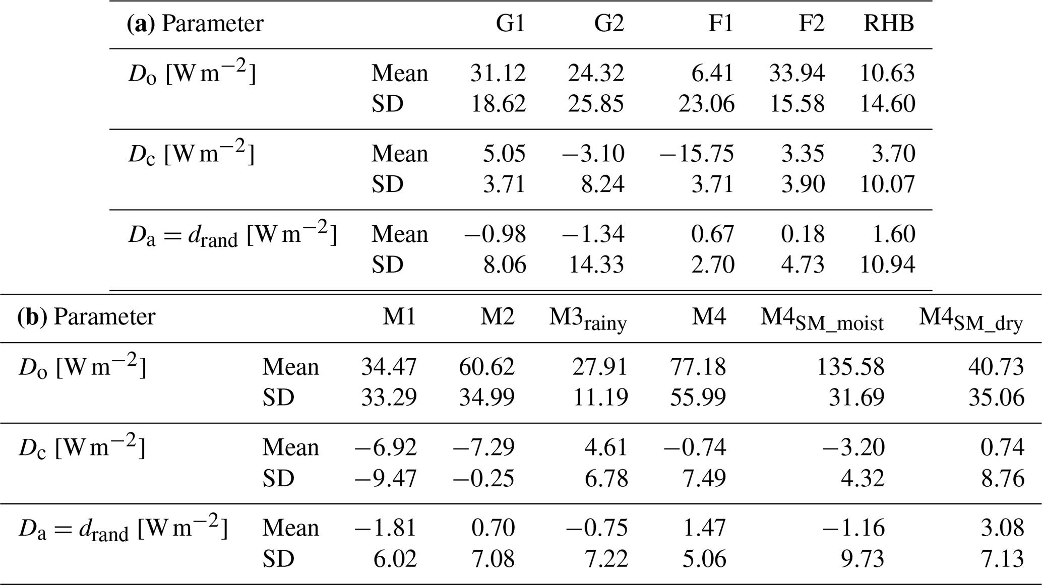
For all stations, the Do averages are positive, i.e., the LY observations are higher on average than the EC observations. For the humid stations F1 and RHB, the Do deviations are below the measurement accuracy. The Dc and Da values are all below the measurement accuracy (except for F1 in Dc) for the humid as well as the semiarid stations.
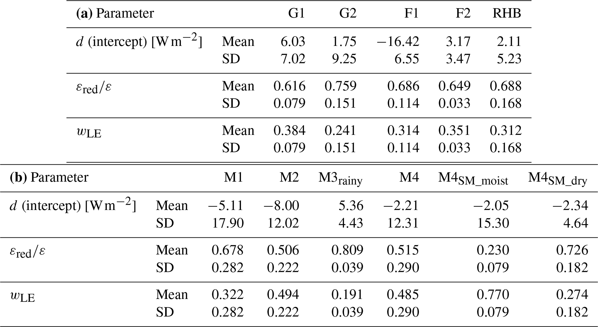
3.3 Parameters obtained by the LY−EC comparison
Table 4a and b presents the parameters d (intercept = systematic deviation), and wLE as obtained by applying Eq. (3). The systematic deviations mean d between LY and EC are all within the measurement accuracy of LY with around and , respectively, except for F1 and (marginally) M2.
Table 4(a) Parameters for humid stations. (b) Parameters for Majadas station; semiarid.
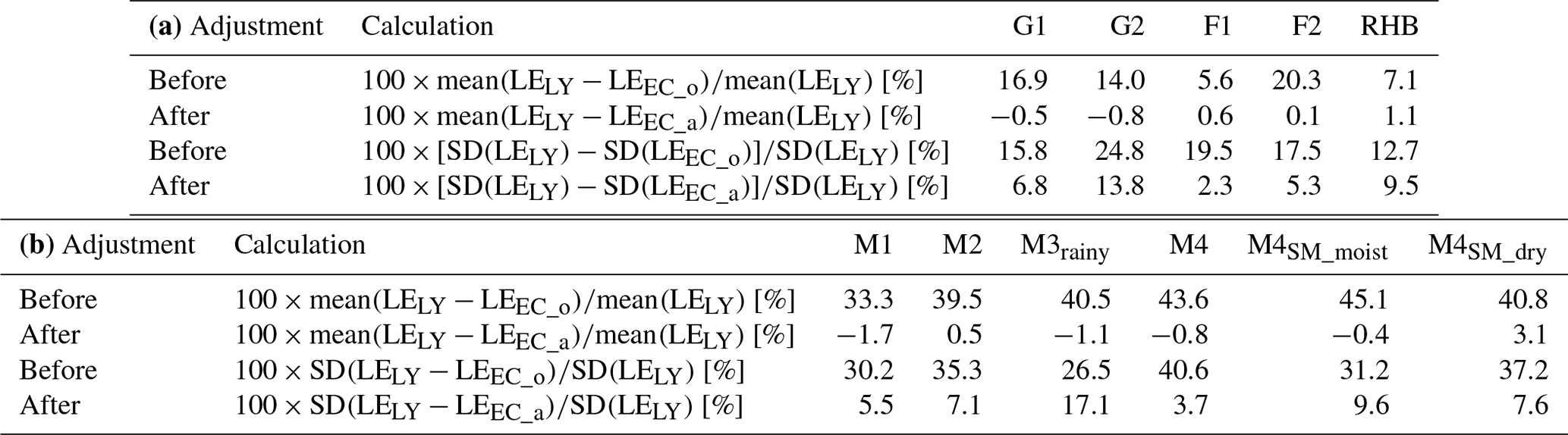
3.4 Reduction of the LY−EC differences by adjustment expressed in percentages
Table 5a and b gives the average and standard deviation differences between the LY and EC values as expressed in percentages of LY. The improvements are made visible by comparing the differences before and after adjustments. As such, they may also be compared to the findings of Chavez and Howell (2009), Ding et al. (2010) and Evett et al. (2012).
Table 5(a) Comparison of the LY−EC differences (means: upper two lines; SDs: lower two lines) before and after adjustment of the EC values, humid. (b) Comparison of the LY−EC differences (means: upper two lines; SDs: lower two lines) before and after adjustment of the EC values, Majadas.
3.5 Differences between the LY and observed, corrected and adjusted EC measurements averaged for daytime hours
Figure 3a and b shows the mean daytime cycle of observed hourly differences LELY−LEEC_o (denoted as Do in Table 3a and b) at the individual stations. The averaged Do differences appear low for the humid data sets and decline towards the afternoon. The Majadas observations are higher and show a tendency to peak around noon for the dry season.

Figure 3Differences : (a) as a function of daytime hours, humid; and (b) as a function of daytime hours, Majadas; red: dry; blue: rainy season.
Figure 4a and b gives the corresponding differences between the LY and the corrected EC measurements, i.e., .
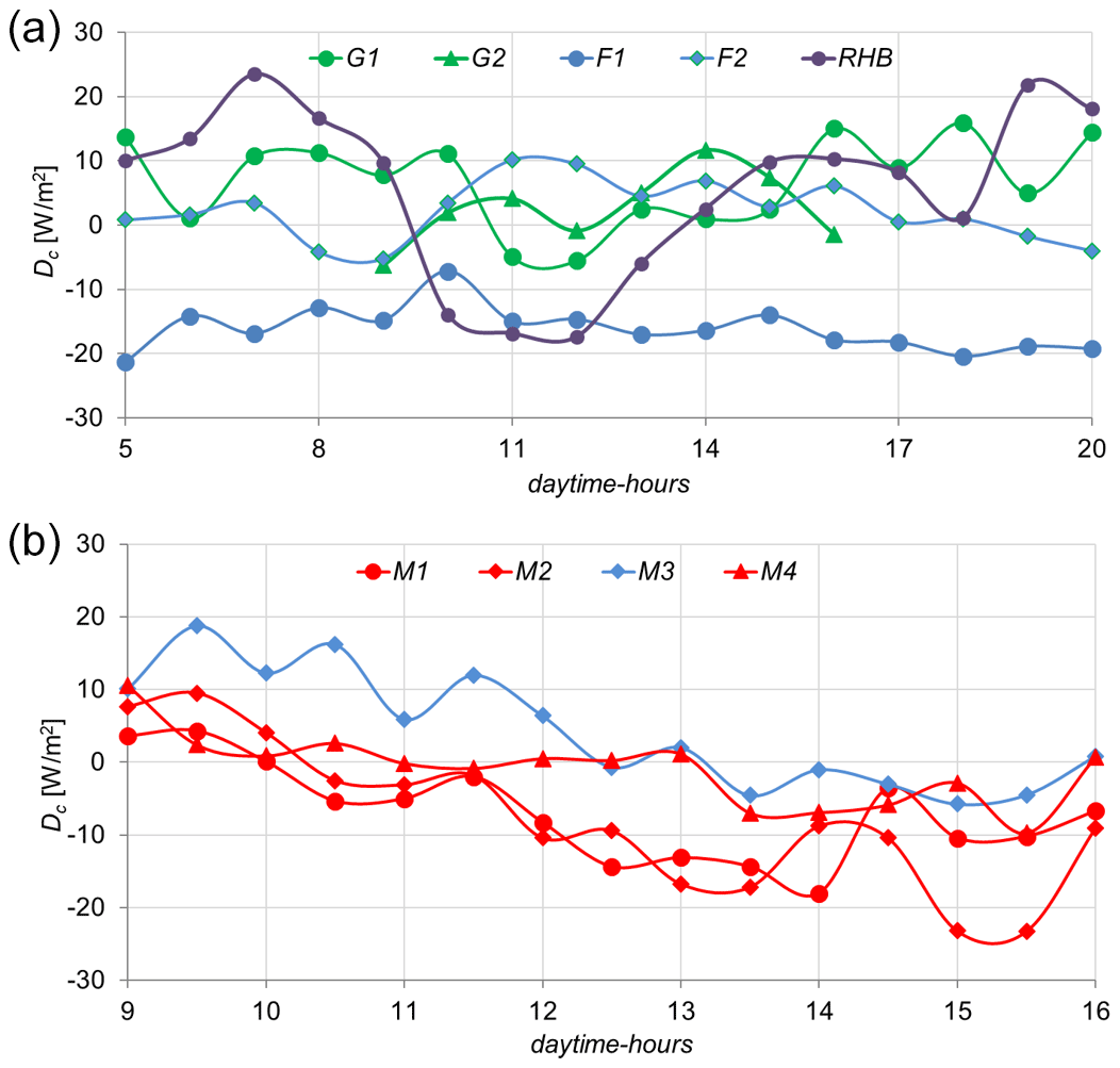
Figure 4Differences : (a) as a function of daytime hours, humid; and (b) as a function of daytime hours, Majadas; red: dry; blue: rainy season.
Figure 5a and b demonstrates the Da values as differences between the LY and adjusted EC measurements (LEEC_a), respectively, and the random deviations drand. The Da differences for all stations are mostly within the LY measurement accuracy of and , respectively, and may be neglected.

Figure 5Differences : (a) as a function of daytime hours, humid; and (b) as a function of daytime hours, Majadas; red: dry; blue: rainy season.
3.6 Systematic deviations averaged for daytime hours
Figure 6a and b presents the systematic deviations d between LELY and LEEC_o. The systematic deviations for the humid stations are mostly within the LY measurement accuracy of and , respectively, and can thus be neglected for F2, G2, RHB, M3 and M4. For F1, the deviations exceed the measurement accuracy quite substantially throughout the daytime period, while the deviations at G1 are larger only in the morning and afternoon and at M1 and M2 from noon until the evening.
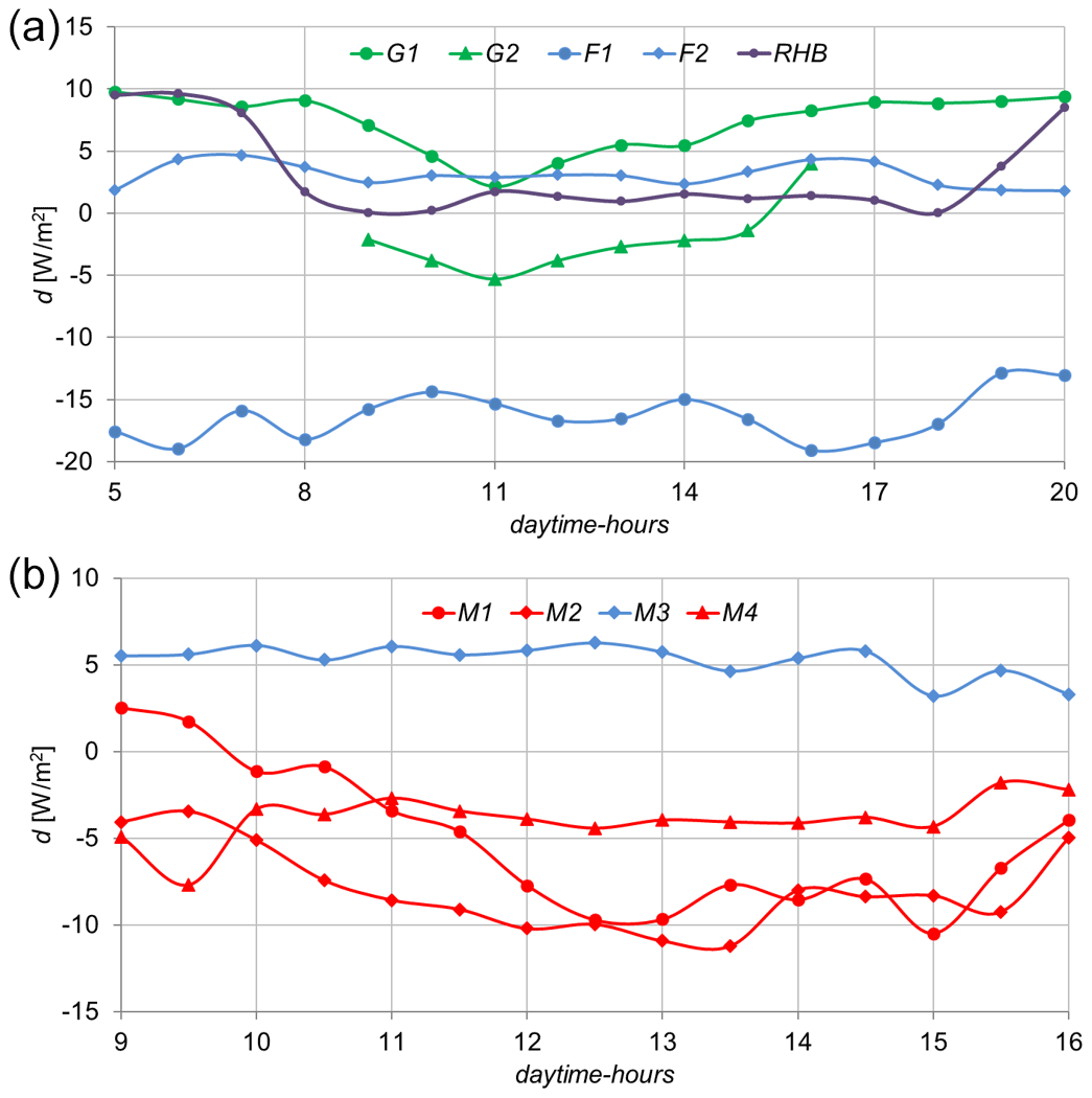
Figure 6Systematic differences d between LELY and adjusted LEEC_a: (a) as a function of daytime hours, humid; and (b) as a function of daytime hours, Majadas red: dry season; blue: rainy season.
3.7 Averaged hourly daytime values for wLE
Figure 7a and b shows the mean course of wLE during daytime hours using the average of all wLE values at a specific hour. The number of bins used in Fig. 7a per station varies from 6 (F1), 8 (F2, G2, RHB) to 14 (G1). The number of bins used for Majadas in Fig. 7b varies from 5 to 12 depending on the used period. We distinguish between the drying periods (about March to August) in red and yellow as well as the one “rainy” period M3 (end of August 2017 to beginning of January 2018) in blue. Figure 7b also splits M4 into a period with “high soil moisture” (20 April to 23 June, yellow line with blue triangles) and a “low soil moisture” (1 July to 4 September, yellow line with yellow triangles). Both periods are under high temperatures and very sparse rainfall. For soil moisture, see Fig. 8b.

Figure 7Averaged daytime hours values for LE-weights wLE: (a) as a function of daytime hours, humid; and (b) as a function of daytime hours, Majadas red: dry; blue: rainy season. M4 is split into the period “high soil moisture” (20 April to 23 June, yellow line, blue triangles) and “low soil moisture” (1 July and 4 September, yellow line, yellow triangles).
All humid averaged values of daytime hours of wLE are roughly within the range of around 0.2 and 0.4. Their standard deviation is highest in the hours around noon (not shown), which relates to the fact that the absolute differences between LELY and LEEC observations are comparably small during stable to weakly unstable conditions in the morning and evening. For Majadas, variations in the various datasets are higher, especially for the drying period (i.e., no rainfall, but still high soil moisture) of M4 (topmost line in Fig. 7b).
3.8 Temporal patterns
3.8.1 wLE in time
Figure 8a and b shows two different situations for the development of wLE in time under varying soil moisture. While Fig. 8a presents a limited dry period under humid conditions (G1), Fig. 8b demonstrates a gradually drying situation over 212 days (20 April to 4 September 2018) for M4.
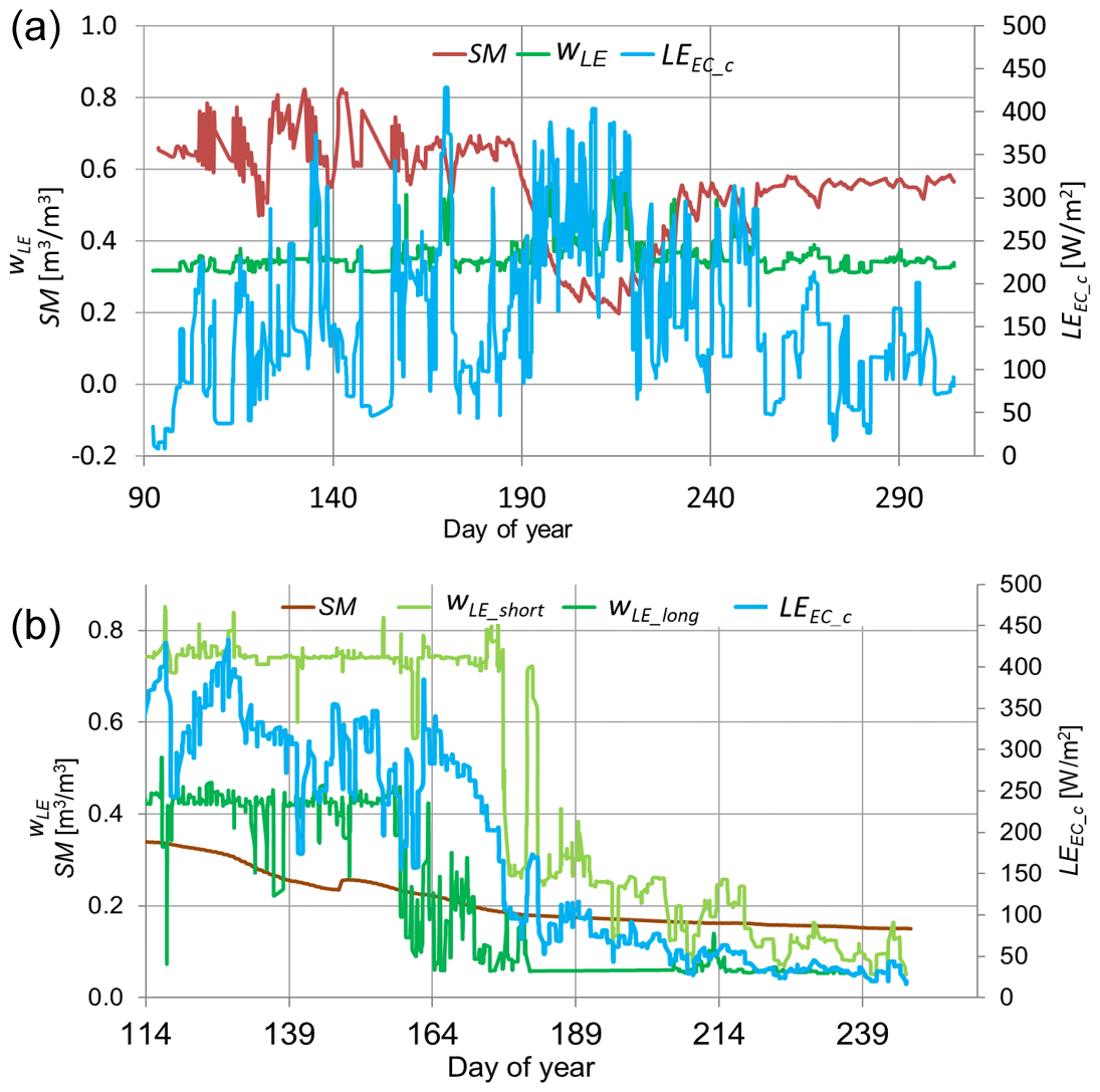
Figure 8(a) Development of wLE (smoothed, dark green), LEEC_c (smoothed, blue) and soil moisture (brown) including a dry spell in 2013 for G1, humid. All data shown are measured from 05:00 to 20:00. A moving median filter with a window length of 11 h was used for smoothing the wLE and LE data. (b) Development of wLE (smoothed, light green) results from values measured between 09:00 and 16:00, the lower wLE (smoothed, dark green) results from estimates from 05:00–09:00 and 16:00–20:00 and measurements between 09:00–16:00 (see Sect. 2.4), and corrected LEEC_c (smoothed, blue) along with soil moisture (SM, brown) from 21 April to 4 September 2018 for M4, semiarid. A moving median filter with a window length of 11 h was used for smoothing the wLE and LE data.
3.8.2 LY–EC deviations in time
Figure 9a and b illustrates the EC deviations from the LY values before (light green) and after (blue) EC adjustments along the analyzed time period for F2 (7a) and M4 (7b). They again demonstrate the remaining high variation.
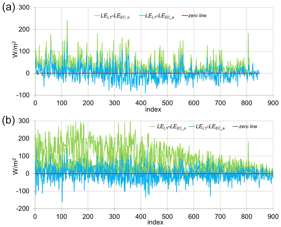
Figure 9(a) EC deviations from LY observations before (green) and after (blue) EC adjustments along observation period for station F2. (b) EC deviations from the LY observations before (green) and after (blue) EC adjustments along observation period for station M4.
The method applied offers two results: (1) corrected LEEC_c values as given by and (2) adjusted LEEC_a values as given by . One may consider LEEC_c as weakly linked to the LY measurements via the wL regression and LEEC_a as strongly linked to LELY via both wLE as well as d. Differences between the two mostly range within the measurement accuracies (Table 3a and b).
In general, LY measured data are higher than data based on the EC method. This is in accordance with the literature (e.g., Chavez and Howell, 2009). They differ substantially less in humid climate with around 10 to 30 W m−2 (0.35 to 1.0 mm d−1) than at the Majadas station with around 30 to 60 W m−2 (1.0 to 2.1 mm d−1).
The adjustment of the EC to the LY data expressed by the differences Da hint at a nearly perfect match for the means (Table 3a and b). They are all in the range of the measurement accuracies. All SDs given by the difference SD(LELY)−SD(LEEC_a), respectively SD(LEEC_c), increase with adjustments, but remain less than SD(LELY) (see the SDs for Do and Da values in Table 3a and b). The difference between SD(LELY) and SD(LEEC_o) gets bigger, since SD(LEEC_o) gets smaller after correction, whereas SD(LELY) remains the same.
The effectiveness of our method is demonstrated by comparing our results given in Table 5a and b with the following previously published results:
-
Chavez and Howell (2009) with reductions of LY–EC differences from −28.8 % to 6.2 % and from −26.0 % to −12.3 %, respectively, with an accuracy of and , respectively
-
Evett et al. (2012), mentioning LEEC measurement errors within ≈55 to 78 W m−2, which were reduced after forced closure of the energy gap to LELY and LEEC differences between −17.4 % and −18.7 %
-
Ding et al. (2010), stating that differences between the LY and EC measurements could be reduced from −22.4 % to −6.2 %.
It is surprising that the systematic deviations d between the LY and EC measurements (Table 4a and b) are on average within the measurement accuracy with the exception of F1 and (marginally) M2. For the humid regions d is positive (four cases) as well as negative (one case). For Majadas d is positive only for M3, measured during the rainy season. For M4 the d values are distinctly below measurement accuracy (Table 4b; Fig. 6b). One could expect a more pronounced difference of d for the two different measurement devices (RHB and lower boundary-controlled lysimeters).
The energy gaps are in the range of 25 to 100 W m−2 for the humid stations. They are much higher for Majadas with around 120 to 180 W m−2. The gaps reduce to about 50 % to 80 % after partial energy closure. They appear rather constant (around 70 %) for the humid regions and vary more for Majadas, for which the most striking variations, i.e., 23 % and 72.6 % occur with M4 during high and low soil moisture, respectively (Table 4a and b, lines εred).
The calculated wLE values appear nearly independent of daytime hours (Fig. 7a and b). Data from the humid climate gave hourly averaged wLE values within a surprisingly narrow range of 0.2 to 0.4. The corresponding values for Majadas show wider variations. During the non-rainy season, they differ more substantially for M4 with high soil moisture (wLE around 0.78) and low soil moisture (wLE around 0.25). This discrepancy of wLE is mitigated by extending the daily time window of the Majadas data (Sect. 2.4).
The SDs of wLE for daytime hour averages change little, with a tendency of smaller values in the morning and evening. This relates to small absolute values of evaporation during stable or weakly unstable conditions.
The value of wLE seems partly positively correlated to the magnitude of evaporation. This correlation is indicated in Fig. 8b, where a drop in wLE follows LEEC_c.
We could not find any explanation for the unexpected drop of d values for G2 (Fig. 6a).
The applied partial closure gives, according to our knowledge, the first fully rational method to partially close the energy gap and a more detailed description of the correlations between the LY and EC observations. The method gives two results for improved LEEC estimates, one weakly linked and one strongly linked to the LELY readings. Their differences appear negligible in view of the inaccuracies of the input data. The method also allows a distinction between systematic and random deviations, probably for the first time. The wLE weight averages are rather stable during daytime. The systematic deviations and random deviations (Table 4a and b) are mostly below or very close to measurement accuracies.
In the future, one should try to increase the temporal resolution of the LY-EC comparison. As a first step we recommend performing the comparison of the LY and EC measurements based on 5 to 10 min lysimeter intervals and center the averaging window accordingly on the EC high-frequency data. We thereby expect an improvement of the accuracy of wLE, d and drand estimates. The benefit of using more highly resolved lysimeter data is described in Ruth et al. (2018).
In the long term, one may think of improving measurement accuracies of relevant input data. Lysimeter measurements should include negative values (condensation) and consider the influence of wind. The former can be realized by including rain observations on a high temporal scale to identify a mass increase in the absence of rain, i.e., dew formation (Ruth et al., 2018). If a high-precision lysimeter capable of resolving evaporation as well as condensation is available complementary to an EC setup, LE can directly be obtained from the lysimeter. As long as no improvements are realized, as a pragmatic solution for full energy balance closure we recommend closing by attributing one third of the gap ε to each of the three weights. This is common practice in land surveying. This recommendation is supported by the fact that we found generally rather constant wLE values between 0.2 and 0.4 during the daytime.
We also recommend testing high-quality flag 0 datasets (Mauder et al., 2013) for plausibility by the out-of-bound method, which may be derived from Wohlfahrt and Widmoser (2013).
The method proposed here may also be applied if reliable sap flow measurements are available instead of lysimeter observations. We guess that an adoption of our method may apply to partial energy closure by heat fluxes if surface temperatures estimates are known from telemetry.
The data basis for the presented analyses is available at https://doi.org/10.5281/zenodo.3957208 (Mauder et al., 2020), https://doi.org/10.3929/ethz-b-000420733 (Michel et al., 2020) and https://doi.org/10.5281/zenodo.3964082 (Widmoser et al., 2020). The datasets consist of the half-hourly or hourly time series of lysimeter and eddy covariance evaporation, respectively, as well as ancillary data described in the text.
PW initiated the study, conducted the analyses and wrote a first version of the manuscript. DM revised the manuscript and put it into shape for publication.
The authors declare that they have no conflict of interest.
We are grateful to Matthias Mauder and Ralf Kiese, Institute of Technology, KIT, Germany; Oscar Perez-Priego, Max Planck Institute for Biogeochemistry, Germany; and Sonia I. Seneviratne and Martin Hirschi, Institute for Atmospheric and Climate Science, ETH Zurich, Switzerland for the data as well as Georg Wohlfahrt, Institute for Ecology, University of Innsbruck, Austria, for support. The Graswang and Fendt sites are part of the TERENO observatory, which is funded by the Helmholtz Association and the Federal Ministry of Education and Research. Majadas lysimeter data were supported by the Alexander von Humboldt Foundation that supported the research with the Max Planck Prize to Markus Reichstein. For the data collection we thank Arnaud Carrara (CEAM, Valencia), Oscar Perez-Priego, Tarek El-Madany, Olaf Kolle and Mirco Migliavacca (Max Planck Institute for Biogeochemistry).
This paper was edited by Miriam Coenders-Gerrits and reviewed by two anonymous referees.
Alfieri, J., Kustas, W., Prueger, J., Hipps, L., Evett, J., Basara, B., Neale, Ch., French, A., Colaizzi, P., Agam, N., Cosh, M., Chavez, J., and Howell, T.: On the discrepancy between eddy covariance and lysimetry-based surface flux measurements under strongly advective conditions, Adv. Water Resour., 50, 62–78, 2012.
Charuchittipan, D., Babel, W., Mauder, M., Leps, J.-P., and Foken, T.: Extension of the Averaging Time in Eddy-Covariance Measurements and Its Effect on the Energy Balance Closure, Bound.-Layer Meteorol., 152, 303–327, https://doi.org/10.1007/s10546-014-9922-6, 2014.
Chavez, J. and Howell, T.: Evaluating eddy covariance cotton ET measurements in an advective environment with large weighing lysimeters, Irrig. Sci., 28, 35–50, 2009.
Ding, R., Kang, S., Li, F., Zhang, Y., Tong, L., and Sun, Q.: Evaluating eddy covariance method by large-scale weighing lysimeter in a maize field of northwest China, Agric. Water Manage., 98, 87–95, 2010.
Endrizzi, S., Gruber, S., Dall'Amico, M., and Rigon, R.: GEOtop 2.0: simulating the combined energy and water balance at and below the land surface accounting for soil freezing, snow cover and terrain effects, Geosci. Model Dev., 7, 2831–2857, https://doi.org/10.5194/gmd-7-2831-2014, 2014.
Evett, S., Schwartz, R., Howell, T., Baumhardt, L., and Copeland, K.: Can weighing lysimeter ET represent surrounding field ET enough to test flux station measurements of daily and sub-daily ET?, Adv. Water Resour., 50, 79–90, 2012.
Foken, T.: The energy balance closure problem: an overview, Ecol. Appl., 18, 1351–1367, https://doi.org/10.1890/06-0922.1, 2008.
Foken, T., Aubinet, M., Finnigan, J. J., Leclerc, M. Y., Mauder, M., and Paw, K. T.: Results of a panel discussion about the energy balance closure correction for trace gases, B. Am. Meteorol. Soc., 92, ES13–ES18, https://doi.org/10.1175/2011BAMS3130.1, 2011.
Gebler, S., Hendricks Franssen, H.-J., Pütz, T., Post, H., Schmidt, M., and Vereecken, H.: Actual evapotranspiration and precipitation measured by lysimeters: a comparison with eddy covariance and tipping bucket, Hydrol. Earth Syst. Sci., 19, 2145–2161, https://doi.org/10.5194/hess-19-2145-2015, 2015.
Hirschi, M., Michel, D., Lehner, I., and Seneviratne, S. I.: A site-level comparison of lysimeter and eddy covariance flux measurements of evapotranspiration, Hydrol. Earth Syst. Sci., 21, 1809–1825, https://doi.org/10.5194/hess-21-1809-2017, 2017.
Leuning, R., Van Gorsel, E., Massman, W. J., and Isaac, P. R.: Reflections on the surface energy imbalance problem, Agr. Forest Meteorol., 156, 65–74, https://doi.org/10.1016/j.agrformet.2011.12.002, 2012.
Mauder, M., Kiese, R., and Widmoser, P.: Evapotranspiration data of the TERENO sites Graswang and Fendt for 2013 and 2014 measured by eddy-covariance and lysimeters, Zenodo, https://doi.org/10.5281/zenodo.3957208, 2020.
Widmoser, P., Perez-Priego, O., El-Madany, T. S., Carrara, A., Kolle, O., Hertel, M., López-Jimenez, R., Reichstein, M., and Migliavacca, M.: Lysimeters data from Windmoser and Michel 2020, Zenodo, https://doi.org/10.5281/zenodo.3964082, 2020.
Mauder, M., Cuntz, M., Drüe, C., Graf, A., Rebmann, C., Schmid, H. P., Schmidt, M., and Steinbrecher, R.: A strategy for quality and uncertainty assessment of long-term eddy-covariance measurements, Agr. Forest Meteorol. 169, 122–135, https://doi.org/10.1016/j.agrformet.2012.09.006, 2013.
Mauder, M., Genzel, S., Fu, J., Kiese, R, Soltani, M, Steinbrecher, R., Zeeman, M, Banerjee, T., De Roo, F., and Kunstmann, H.: Evaluation of two energy balance closure adjustment methods by independent evapotranspiration estimates from lysimeters and hydrological simulations, Hydrol. Process., 32, 39–50, 2018.
Mauder, M., Foken, T., and Cuxart, J.: Surface-Energy-Balance Closure over Land: A Review, Bound.-Layer Meteorol., 177, 395–426, 2020.
Meissner, R., Seeger, J., Rupp, H., Seyfarth, M., and Borg, H.: Measurement of dew, fog, and rime with a high-precision gravitation lysimeter, J. Plant Nutr. Soil Sci., 170, 335–344, 2007.
Michel, D., Seneviratne, S. I., and Widmoser, P.: Eddy-covariance and lysimeter data of evapotranspiration at Rietholzbach (Widmoser & Michel 2020, HESS), ETH research collection, https://doi.org/10.3929/ethz-b-000420733, 2020.
Migliavacca, M., Perez-Priego, O., Rossini M., El-Madany, T. S., Moreno, G., van der Tol, Ch., Rascher, U., Berninger, A., Bessenbacher, V., Burkart, A., Carrara, A., Fava, F., Guan, J.-H., Hammer, T. W., Henkel, K., Juarez-Alcalde, E., Julitta, T., Kolle, O., Martin, M. P., Musavi, T., Pacheco-Labrador, J., Pierez-Burgueño, A., Wutzler, Th., Zaehle, S., and Reichstein, M.: Plant functional traits and canopy structure control the relationship between photosynthetic CO2 uptake and far-red sun-induced fluorescence in a Mediterranean grassland under different nutrient availability, New Phytol., 214, 1078–1091, https://doi.org/10.1111/nph.14437, 2017.
Perez-Priego, O., El-Madany, T. S., Migliavacca, M., Kowalski, A. S., Jung, M., Carrara, A., Kolle, O., Martín, M. P., Pacheco-Labrador, J., Moreno, G., and Reichstein, M.: Evaluation of eddy covariance latent heat fluxes with independent lysimeter and sapflow estimates in a Mediterranean savannah ecosystem, Agr. Forest Meteorol., 236, 87–99, https://doi.org/10.1016/j.agrformet.2017.01.009, 2017.
Ruth, C. E., Michel, D., Hirschi, M., and Seneviratne, S. I.: Comparative Study of a Long-Established Large Weighing Lysimeter and a State-of-the-Art Mini-lysimeter, Vadose Zone J., 17, 1–10, https://doi.org/10.2136/vzj2017.01.0026, 2018.
Seneviratne, S. I., Lehner, I., Gurtz, J., Teuling, A. J., Lang, H., Moser, U., Grebner, D., Menzel, L., Schroff, K., Vitvar, T., and Zappa, M.: Swiss prealpine Rietholzbach research catchment and lysimeter: 32 year time series and 2003 drought event, Water Resour. Res., 48, W06526, https://doi.org/10.1029/2011WR011749, 2012.
Widmoser, P. and Wohlfahrt, G.: Attributing the energy imbalance by concurrent lysimeter and eddy covariance evapotranspiration measurements, Agr. Forest Meteorol., 263, 287–291, 2018.
Wilson, K., Goldstein, A., Falge, E., Aubinet, M., Baldocchi, D., Berbigier, P., Bernhofer, C., Ceulemans, R., Dolman, H., Field, C., Grelle, A., Ibrom, A., Law, B. E., Kowalski, A., Meyers, T., Moncrieff, J., Monson, R., Oechel, W., Tenhunen, J., Valentini, R., and Verma, S.: Energy balance closure at FLUXNET sites, Agr. Forest Meteorol., 113, 223–243, https://doi.org/10.1016/S0168-1923(02)00109-0, 2002.
Wohlfahrt, G. and Widmoser P.: Can an energy balance model provide additional constraints on how to close the energy imbalance?, Agr. Forest Meteorol., 169, 85–91, 2013.
Zacharias, S., Bogena, H., Samaniego, L., Mauder, M., Fuß, R., Pütz, T., Frenzel, M., Schwank, M., Baessler, C., Butterbach-Bahl, K., Bens, O., Borg, E., Brauer, A., Dietrich, P., Hajnsek, I., Helle, G., Kiese, R., Kunstmann, H., Klotz, S., Munch, J. C., Papen, H., Priesack, E., Schmid, H. P., Steinbrecher, R., Rosenbaum, U., Teutsch, G., and Vereecken, H.: A Network of Terrestrial Environmental Observatories in Germany, Vadose Zone J., 10, 955–973, https://doi.org/10.2136/vzj2010.0139, 2011.