the Creative Commons Attribution 4.0 License.
the Creative Commons Attribution 4.0 License.
 | 02 Mar 2021
Behind the scenes of streamflow model performance
Laurène J. E. Bouaziz
Fabrizio Fenicia
Guillaume Thirel
Tanja de Boer-Euser
Joost Buitink
Claudia C. Brauer
Jan De Niel
Benjamin J. Dewals
Gilles Drogue
Benjamin Grelier
Lieke A. Melsen
Sotirios Moustakas
Jiri Nossent
Fernando Pereira
Eric Sprokkereef
Jasper Stam
Albrecht H. Weerts
Patrick Willems
Hubert H. G. Savenije
Markus Hrachowitz
Streamflow is often the only variable used to evaluate hydrological models. In a previous international comparison study, eight research groups followed an identical protocol to calibrate 12 hydrological models using observed streamflow of catchments within the Meuse basin. In the current study, we quantify the differences in five states and fluxes of these 12 process-based models with similar streamflow performance, in a systematic and comprehensive way. Next, we assess model behavior plausibility by ranking the models for a set of criteria using streamflow and remote-sensing data of evaporation, snow cover, soil moisture and total storage anomalies. We found substantial dissimilarities between models for annual interception and seasonal evaporation rates, the annual number of days with water stored as snow, the mean annual maximum snow storage and the size of the root-zone storage capacity. These differences in internal process representation imply that these models cannot all simultaneously be close to reality. Modeled annual evaporation rates are consistent with Global Land Evaporation Amsterdam Model (GLEAM) estimates. However, there is a large uncertainty in modeled and remote-sensing annual interception. Substantial differences are also found between Moderate Resolution Imaging Spectroradiometer (MODIS) and modeled number of days with snow storage. Models with relatively small root-zone storage capacities and without root water uptake reduction under dry conditions tend to have an empty root-zone storage for several days each summer, while this is not suggested by remote-sensing data of evaporation, soil moisture and vegetation indices. On the other hand, models with relatively large root-zone storage capacities tend to overestimate very dry total storage anomalies of the Gravity Recovery and Climate Experiment (GRACE). None of the models is systematically consistent with the information available from all different (remote-sensing) data sources. Yet we did not reject models given the uncertainties in these data sources and their changing relevance for the system under investigation.
- Article
(4445 KB) - Full-text XML
-
Supplement
(500 KB) - BibTeX
- EndNote


Hydrological models are valuable tools for short-term forecasting of river flows and long-term predictions for strategic water management planning, but also to develop a better understanding of the complex interactions of water storage and release processes at the catchment scale. In spite of the wide variety of existing hydrological models, they mostly include similar functionalities of storage, transmission and release of water to represent the dominant hydrological processes of a particular river basin (Fenicia et al., 2011), differing mostly only in the detail of their parameterizations (Gupta et al., 2012; Gupta and Nearing, 2014; Hrachowitz and Clark, 2017).
In all of these models, each individual model component constitutes a separate hypothesis of how water moves through that specific part of the system. Frequently, the individual hypotheses remain untested. Instead, only the model output, i.e., the aggregated response of these multiple hypotheses, is confronted with data of the aggregated response of a catchment to atmospheric forcing. Countless applications of different hydrological models in many different regions across the world over the last decades have shown that these models often provide relatively robust estimates of streamflow dynamics, for both calibration and evaluation periods. However, various combinations of different untested individual hypotheses can and do lead to similar aggregated outputs, i.e., model equifinality (Beven, 2006; Clark et al., 2016).
To be useful for any of the above applications, it is thus of critical importance that not only the aggregated but also the individual behaviors of the respective hypotheses are consistent with their real-world equivalents. Given the complexity and heterogeneity of natural systems together with the general lack of suitable observations, this remains a major challenge in hydrology (e.g., Jakeman and Hornberger, 1993; Beven, 2000; Gupta et al., 2008; Andréassian et al., 2012).
Studies have addressed the issue by constraining the parameters of specific models through the use of additional data sources besides streamflow. Beven and Kirkby (1979), Güntner et al. (1999) and Blazkova et al. (2002) mapped saturated contributing areas during field surveys to constrain model parameters, while patterns of water tables in piezometers were used by Seibert et al. (1997), Lamb et al. (1998) and Blazkova et al. (2002). Other sources include satellite-based total water storage anomalies (e.g., Winsemius et al., 2006; Werth and Güntner, 2010; Yassin et al., 2017), evaporation (e.g., Livneh and Lettenmaier, 2012; Rakovec et al., 2016a; Bouaziz et al., 2018; Demirel et al., 2018; Hulsman et al., 2020), near-surface soil moisture (e.g., Franks et al., 1998; Brocca et al., 2010; Sutanudjaja et al., 2014; Adnan et al., 2016; Kunnath-Poovakka et al., 2016; López López et al., 2017; Bouaziz et al., 2020), snow cover information (e.g., Gao et al., 2017; Bennett et al., 2019; Riboust et al., 2019), or a combination of these variables (e.g., Nijzink et al., 2018; Dembélé et al., 2020). Reflecting the results of many studies, Rakovec et al. (2016b) showed that streamflow is necessary but not sufficient to constrain model components to warrant partitioning of incoming precipitation to storage, evaporation and drainage.
Hydrological simulations are, however, not only affected by model parameter uncertainty, but also by the selection of a model structure and its parameterization (i.e., the choice of equations). Modeling efforts over the last 4 decades have led to a wide variety of hydrological models providing flexibility to test competing modeling philosophies, from spatially lumped model representations of the system to high-resolution small-scale processes numerically integrated to the catchment scale (Hrachowitz and Clark, 2017). Haddeland et al. (2011) and Schewe et al. (2014) compared global hydrological models and found that differences between models are a major source of uncertainty. Nonetheless, model selection is often driven by personal preference and experience of individual modelers rather than detailed model test procedures (Holländer et al., 2009; Clark et al., 2015; Addor and Melsen, 2019).
A suite of comparison experiments tested and explored differences between alternative modeling structures and parameterizations (Perrin et al., 2001; Reed et al., 2004; Duan et al., 2006; Holländer et al., 2009; Knoben et al., 2020). However, these studies mostly restricted themselves to analyses of the models' skills in reproducing streamflow (“aggregated hypothesis”), with little consideration for the model-internal processes (“individual hypotheses”). The Framework for Understanding Structural Errors (FUSE) was one of the first initiatives towards a more comprehensive assessment of model structural errors, with special consideration given to individual hypotheses (Clark et al., 2008).
Subsequent efforts towards more rigorous testing of competing model hypotheses, partially based on internal processes, include Smith et al. (2012a, b), who tested multiple models for their ability to reproduce in situ soil moisture observations as part of the Distributed Model Intercomparison Project 2 (DMIP2). They found that only 2 out of 16 models provided reasonable estimates of soil moisture. In a similar effort, Koch et al. (2016) and Orth et al. (2015) also compared modeled soil moisture to in situ observations of soil moisture for a range of hydrological models in different environments. In contrast, Fenicia et al. (2008) and Hrachowitz et al. (2014) used groundwater observations to test individual components of their models. There are actually relatively few studies that comprehensively quantified differences in internal process representation by simultaneously analyzing multiple models and multiple state and flux variables.
Here, in this model comparison study, we instead use globally available remote-sensing data to evaluate five different model state and flux variables of 12 process-based models with similar overall streamflow performance, which are calibrated by several research groups following an identical protocol. The calibration on streamflow was conducted in our previous study (de Boer-Euser et al., 2017), in which we compared models using hourly streamflow observations, leaving the modeled response of internal processes unused.
In a direct follow-up to the above study, we here hypothesize that process-based models with similar overall streamflow performance rely on similar representations of their internal states and fluxes. We test our hypothesis by simultaneously quantifying the differences in the magnitudes and dynamics of five internal state and flux variables of 12 models, in a comprehensive and systematic way. Our primary aim is to test whether models calibrated to streamflow with similar high-performance levels in reproducing streamflow follow similar pathways to do so, i.e., represent the system in a similar way. A secondary objective is to evaluate the plausibility of model behavior by introducing a set of “soft” measures based on expert knowledge in combination with remote-sensing data of evaporation, snow cover, soil moisture and total water storage anomalies.
We test our hypothesis using data from three catchments in the Belgian Ardennes; all of them are part of the Meuse River basin in northwestern Europe: the Ourthe upstream of Tabreux (ID1), the nested Ourthe Orientale upstream of Mabompré (ID2) and the Semois upstream of Membre-Pont (ID3), as shown in Fig. 1. The Ardennes Massif and Plateau are underlain by relatively impermeable metamorphic Cambrian rock and Early Devonian sandstone. The pronounced streamflow seasonality of these catchments is driven by high summer and low winter evaporation (defined here as the sum of all evaporation components including transpiration, soil evaporation, interception, sublimation and open water evaporation when applicable), as precipitation is relatively constant throughout the year. Snow is not a major component of the water balance but occurs almost every year with mean annual number of days with precipitation as snow estimated between 35 and 40 d yr−1 (Royal Meteorological Institute Belgium, 2015). Even if mean annual snow storage is relatively small, snow can be important for specific events, for example, in 2011, when rain on snow caused widespread flooding in these catchments.
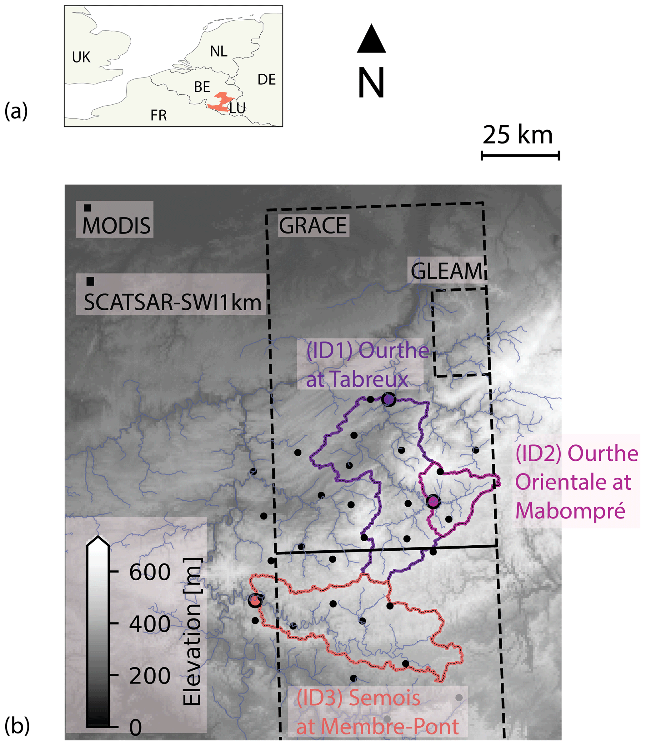
Figure 1(a) Location of the study catchments in Belgium, northwestern Europe. (b) Digital elevation model and catchments of the Ourthe upstream of Tabreux (ID1), Ourthe Orientale upstream of Mabompré (ID2) and Semois upstream of Membre-Pont (ID3). Pixel size of GRACE, GLEAM, MODIS and SCATSAR-SWI1km. Colored dots are the streamflow gauging locations, and black dots are the precipitation stations.
The rain-fed Ourthe River at Tabreux (ID1) is fast-responding due to shallow soils and steep slopes in the catchment. Agriculture is the main land cover (27 % crops and 21 % pasture), followed by 46 % forestry and 6 % urban cover in an area of 1607 km2 and an elevation ranging between 107 and 663 m (European Environment Agency, 2000; de Boer-Euser et al., 2017). Mean annual precipitation, potential evaporation and streamflow are 979, 730 and 433 mm yr−1, respectively, for the period 2001–2017.
Nested within the Ourthe catchment (ID1), the Ourthe Orientale upstream of Mabompré (ID2) is characterized by a narrow elevation range from 294 to 662 m, with 65 % of the catchment falling within a 100 m elevation band, making this catchment suitable for analyzing snow processes modeled by lumped models. The Ourthe Orientale upstream of Mabompré has an area of 317 km2, which corresponds to 20 % of the Ourthe area upstream of Tabreux and has similar land cover fractions. Mean annual precipitation, potential evaporation and streamflow for the period 2001–2017 are also relatively similar, at 1052, 720 and 462 mm yr−1, respectively.
Forest is the main land cover in the Semois upstream of Membre-Pont (ID3), at 56 %, followed by agriculture (18 % pasture and 21 % crop) and 5 % urban cover. The Semois upstream of Membre-Pont is 24 % smaller than the Ourthe upstream of Tabreux, at 1226 km2, and elevation ranges between 176 and 569 m. Mean annual precipitation, potential evaporation and streamflow are, respectively, 38 %, 4 % and 46 % higher in the Semois at Membre-Pont, at 1352, 759 and 634 mm yr−1.
3.1 Hydrological and meteorological data
Hourly precipitation gauge data are provided by the Service Public de Wallonie (Service Public de Wallonie, 2018) and are spatially interpolated using Thiessen polygons. Daily minimum and maximum temperatures are retrieved from the 0.25∘ resolution gridded E-OBS dataset (Haylock et al., 2008) and disaggregated to hourly values by linear interpolation using the timing of daily minimum and maximum radiation at Maastricht (Royal Netherlands Meteorological Institute, 2018). Daily potential evaporation is calculated from daily minimum and maximum temperatures using the Hargreaves formula (Hargreaves and Samani, 1985) and is disaggregated to hourly values using a sine function during the day and no evaporation at night. We use the same forcing for 2000–2010 as in the previous comparison study (de Boer-Euser et al., 2017) and follow the same approach to extend the meteorological dataset for the period 2011–2017. Uncertainty in meteorological data is not explicitly considered, but our primary aim is to compare the models forced with identical data. Observed hourly streamflow data for the Ourthe at Tabreux, Ourthe Orientale at Mabompré and Semois at Membre-Pont are provided by the Service Public de Wallonie for the period 2000–2017.
3.2 Remote-sensing data
3.2.1 GLEAM evaporation
The Global Land Evaporation Amsterdam Model (GLEAM, Miralles et al., 2011; Martens et al., 2017) provides daily estimates of land evaporation by maximizing the information recovery on evaporation contained in climate and environmental satellite observations. The Priestley and Taylor (1972) equation is used to calculate potential evaporation for bare soil, short canopy and tall canopy land fractions. Actual evaporation is the sum of interception and potential evaporation reduced by a stress factor. This evaporative stress factor is based on microwave observations of vegetation optical depth and estimates of root-zone soil moisture in a multi-layer water-balance model. Interception evaporation is estimated separately using a Gash analytical model and only depends on precipitation and vegetation characteristics. GLEAM v3.3a relies on reanalysis net radiation and air temperature from the European Centre for Medium-Range Weather Forecasts (ECMWF) ERA5 data, satellite and gauge-based precipitation, satellite-based vegetation optical depth, soil moisture and snow water equivalent. The data are available at 0.25∘ resolution (Fig. 1b) and account for subgrid heterogeneity by considering three land cover types. We spatially average GLEAM interception and total actual evaporation estimates over the Ourthe catchment upstream of Tabreux for the period 2001–2017.
3.2.2 MODIS snow cover
The Moderate Resolution Imaging Spectroradiometer (MODIS) AQUA (MYD10A1, version 6) and TERRA (MOD10A1, version 6) satellites provide daily maps of the areal fraction of snow cover per 500 m × 500 m cell (Fig. 1b) based on the Normalized Difference Snow Index (Hall and Riggs, 2016a, b). For each day, AQUA and TERRA observations are merged into a single observation by taking the mean fraction of snow cover per day. The percentage of cells with a fractional snow cover larger than zero and fraction of cells without missing data (i.e., due to cloud cover) for the catchment of the Ourthe Orientale upstream of Mabompré is calculated for each day. For this study, we disregard observations during the summer months (JJA, when temperatures did not drop below 4 ∘C) and only use daily observations in which at least 40 % of the catchment area has snow cover retrievals not affected by clouds, implying that we have 1463 valid daily observations of mean fractional snow cover. This corresponds to 32 % of all observations of the Ourthe Orientale catchment upstream of Mabompré between 2001 and 2017.
3.2.3 SCATSAR-SWI1km Soil Water Index
SCATSAR-SWI1km is a daily product of soil water content relative to saturation at a 1 km × 1 km resolution (Fig. 1b) obtained by fusing spatio-temporally complementary radar sensors (Bauer-Marschallinger et al., 2018). Estimates of the moisture content relative to saturation at various depths in the soil, referred to as the Soil Water Index (SWI), are obtained through temporal filtering of the 25 km METOP ASCAT near-surface soil moisture (Wagner et al., 2013) and 1 km Sentinel-1 near-surface soil moisture (Bauer-Marschallinger et al., 2018). The Soil Water Index features as a single parameter the characteristic time length T (Wagner et al., 1999; Albergel et al., 2008). The T value is required to convert near-surface soil moisture observations to estimates of root-zone soil moisture. The T value increases with increasing root-zone storage capacities (Bouaziz et al., 2020), resulting in more smoothing and delaying of the near-surface soil moisture signal. The Copernicus Global Land Service (2019) provides the Soil Water Index for T values of 2, 5, 10, 15, 20, 40, 60 and 100 d. Since Sentinel-1 was launched in 2014, the Soil Water Index is available for the period 2015–2017. We calculate the mean soil moisture over all SCATSAR-SWI1km pixels within the Ourthe upstream of Tabreux for the available period.
3.2.4 GRACE total water storage anomalies
The Gravity Recovery and Climate Experiment (GRACE, Swenson and Wahr, 2006; Swenson, 2012) twin satellites, launched in March 2002, measure the Earth's gravity field changes by calculating the changes in the distance between the two satellites as they move one behind the other in the same orbital plane. Monthly total water storage anomalies (in millimeters) relative to the 2004–2009 time-mean baseline are provided at a spatial sampling of 1∘ (approximately 78 km × 110 km at the latitude of the study region, Fig. 1b) by three centers: U. Texas/Center for Space Research (CSR), GeoForschungsZentrum Potsdam (GFZ) and Jet Propulsion Laboratory (JPL). These centers apply different processing strategies which lead to variations in the gravity fields. These gravity fields require smoothing of the noise induced by attenuated short wavelength. The spatial smoothing decreases the already coarse GRACE resolution even further through signal “leakage” of one location to surrounding areas (Bonin and Chambers, 2013), which increases the uncertainty especially at the relatively small scale of our study catchments. We apply the scaling coefficients provided by NASA to restore some of the signal loss due to processing of GRACE observations (Landerer and Swenson, 2012). The data of the three processing centers are each spatially averaged over the catchments of the Ourthe upstream of Tabreux and the Semois upstream of Membre-Pont for the period April 2002 to February 2017.
3.3 Data uncertainty
The hydrological evaluation data are all subject to uncertainties (Beven, 2019). Streamflow is not measured directly but depends on water level measurements and a rating curve. Westerberg et al. (2016) quantify median streamflow uncertainties of ±12 %, ±24 % and ±34 % for average, high and low streamflow conditions, respectively, using a Monte Carlo sampling approach of multiple feasible rating curves for 43 UK catchments. We sample from these uncertainty ranges to transform the streamflow observations (100 realizations). We then quantify signature uncertainty originating from streamflow data uncertainty using the 100 sampled time series for a selection of streamflow signatures (Sect. 4.2). The 5th–95th uncertainty bounds of median annual streamflow, baseflow and flashiness indices result in ±11 %, ±9 % and ±12 %, respectively. These magnitudes are similar to those reported by Westerberg et al. (2016).
GLEAM evaporation estimates are inferred from models and forcing data which are all affected by uncertainty. Yet uncertainty estimates of GLEAM evaporation are not available. However, GLEAM evaporation was evaluated against FLUXNET data by Miralles et al. (2011). For the nearby station of Lonzee in Belgium, they report similar annual rates and a high correlation coefficient of 0.91 between the daily time series. GLEAM mean annual evaporation was compared to the ensemble mean of five evaporation datasets in Miralles et al. (2016) and shows higher than average values in Europe (of approximately 60 mm yr−1 or 10 % of mean annual rates for our study area). The partitioning of evaporation into different components (transpiration, interception and soil evaporation) differs substantially between different evaporation datasets, as shown by Miralles et al. (2016). GLEAM interception currently only considers tall vegetation and underestimates in situ data (Zhong et al., 2020) and is ∼ 50 % lower than estimates from other datasets (Miralles et al., 2016). These uncertainties underline that GLEAM (and other remote-sensing data) cannot be considered a reliable representation of real-world quantities. However, the comparison of daily dynamics and absolute values of this independent data source with modeled results is still valuable for detecting potential outliers and understanding their behavior. In addition, the different methods used to estimate potential evaporation of GLEAM and our model forcing should not impede us from testing the consistency between the resulting actual evaporation (Oudin et al., 2005).
The most frequent errors within the MODIS snow cover products are due to cloud–snow discrimination problems. Daily MODIS snow maps have an accuracy of approximately 93 % at the pixel scale, with lower accuracy in forested areas and complex terrain and when snow is thin and ephemeral and higher accuracy in agricultural areas (Hall and Riggs, 2007). However, here, MODIS data are used to estimate the number of days with snow at the catchment scale. We expect lower classification errors at the catchment scale as it would require many pixels to be misclassified at the same time. For each day and each pixel of valid MODIS observations, we sample from a binomial distribution with a probability of 93 % that MODIS is correct when the pixel is classified as snow and assume a higher probability of 99 % that MODIS is correct when the pixel is classified as no-snow to prevent overestimation of snow for days without snow (Ault et al., 2006; Parajka and Blöschl, 2006). We repeat the experiment 1000 times in a Monte Carlo procedure. This results in less than ±2 % uncertainty in the number of days when MODIS observes snow at the catchment scale.
The soil water content relative to saturation of SCATSAR-SWI1km is estimated from observed radar backscatter through a change detection approach, which interprets changes in backscatter as changes in soil moisture, while other surface properties are assumed static (Wagner et al., 1999). The degree of saturation of the near surface is given in relative units from 0 % (dry reference) to 100 % (wet reference) and is converted to deeper layers through an exponential filter called the Soil Water Index. The smoothing and delaying effect of the Soil Water Index narrows the range of the near-surface degree of saturation. Therefore, data matching techniques are often used to rescale satellite data to match the variability of modeled or observed data (Brocca et al., 2010), which suggests the difficulty in meaningfully comparing the range of modeled and remote-sensing estimates of root-zone soil moisture content relative to saturation. However, the dynamics of SCATSAR-SWI1km data have been evaluated against in situ stations of the International Soil Moisture Network, despite commensurability issues of comparing in situ point measurements and areal satellite data. Spearman rank correlation coefficients of 0.56 are reported for T values up to 15 d and 0.43 for a T value of 100 d (Bauer-Marschallinger, 2020).
GRACE estimates of total water storage anomalies suffer from signal degradation due to measurement errors and noise. Filtering approaches are applied to reduce these errors but induce leakage of signals from surrounding areas. The uncertainty decreases as the size of the region under consideration increases. However, time series of a single pixel may still be used to compare dynamics and amplitudes of total water storage anomalies despite possible large uncertainty (Landerer and Swenson, 2012). We estimate an uncertainty in total water storage anomalies of ∼ 18 mm in the pixels of our catchments by combining measurement and leakage errors in quadrature, which are both provided for each grid location (Landerer and Swenson, 2012).
4.1 Models and protocol
Eight research groups (Wageningen University, Université de Lorraine, Leuven University, Delft University of Technology, Deltares, Irstea (now INRAE), Eawag and Flanders Hydraulics Research) participated in the comparison experiment and applied one or several hydrological models (Fig. 2). The models include WALRUS (Wageningen Lowland Runoff Simulator, Brauer et al., 2014a, b), PRESAGES (PREvision et Simulation pour l'Annonce et la Gestion des Etiages Sévères, Lang et al., 2006), VHM (Veralgemeend conceptueel Hydrologisch Model, Willems, 2014), FLEX-Topo, which was still under development when it was calibrated for our previous study (Savenije, 2010; de Boer-Euser et al., 2017; de Boer-Euser, 2017), a distributed version of the HBV model (Hydrologiska Byråns Vattenbalansavdelning, Lindström et al., 1997), the SUPERFLEX M2 to M5 models (Fenicia et al., 2011, 2014), dS2 (distributed simple dynamical systems, Buitink et al., 2020), GR4H (Génie Rural à 4 paramètres Horaire, Mathevet, 2005; Coron et al., 2017, 2019) combined with the CemaNeige snow module (Valéry et al., 2014) and NAM (NedborAfstrommings Model, Nielsen and Hansen, 1973). The main differences and similarities between the models in terms of snow processes, root-zone storage, total storage and evaporation processes are summarized in Tables 1–3.
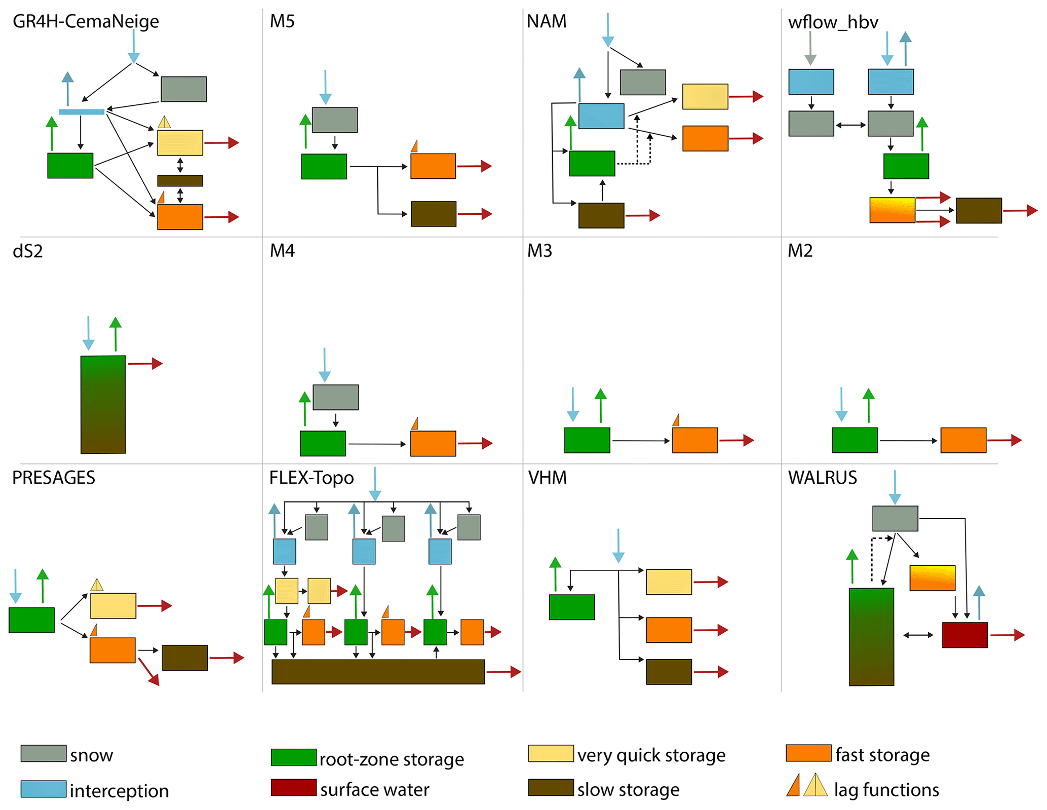
Figure 2Simplified schematic overview of 12 model structures (adapted from de Boer-Euser et al., 2017) with the aim of highlighting similarities and differences between the models. Solid arrows indicate fluxes between stores, while dashed arrows indicate the influence of a state on a flux. Colored arrows indicate incoming or outgoing fluxes, whereas black arrows indicate internal fluxes. The narrow blue rectangle in GR4H indicates the presence of an interception module without interception storage capacity (Table 3). Storages with a color gradient indicate the combination of several components in one reservoir. FLEX-Topo consists of three hydrological response units connected through a shared slow reservoir, and wflow_hbv is a distributed model.
In our previous study (de Boer-Euser et al., 2017), we defined a modeling protocol to limit the degrees of freedom in the modeling decisions of the individual participants (Ceola et al., 2015), allowing us to meaningfully compare the model results. The protocol involved forcing the models with the same input data and calibrating them for the same time period, using the same objective functions. However, participants were free to choose a parameter search method, as we considered it to be part of the modelers' experience with the model, even if this would make comparison less straightforward. The models were previously calibrated using streamflow of the Ourthe at Tabreux (ID1) for the period 2004 to 2007, using 2003 as a warm-up year (de Boer-Euser et al., 2017). The Nash–Sutcliffe efficiencies of the streamflow and the logarithms of the streamflow were simultaneously used as objective functions to select an ensemble of 20 feasible parameter sets to account for parameter uncertainty and ensure a balance between the models' ability to reproduce both high and low flows. The temporal and spatial transferability of the models was tested by evaluating the models in a pre- and post-calibration period and by applying the calibrated model parameter sets to nested and neighboring catchments, including catchment ID2 and ID3 (Klemeš, 1986). Results thereof are presented in de Boer-Euser et al. (2017).
In the current study, we run the calibrated models for an additional period from 2011 to 2017 for the Ourthe at Tabreux (ID1), the Ourthe Orientale at Mabompré (ID2) and the Semois at Membre-Pont (ID3). Note that the calibration (2004–2007) and post-calibration (2008–2017) periods have relatively similar hydro-climatic characteristics in terms of streamflow and overall water balance (Figs. S1 and S2 of the Supplement). The modeling groups have provided simulation results for each catchment in terms of streamflow, groundwater losses/gains, interception evaporation, root-zone evaporation (transpiration and soil evaporation), total actual evaporation, snow storage, root-zone storage and total storage as a sum of all model storage volumes (Table 2) at an hourly time step for the total period 2001–2017. We compare these modeled states and fluxes and evaluate them against their remote-sensing equivalents as further explained in Sects. 4.2 and 4.3. Our results are mainly shown for the Ourthe at Tabreux (ID1), as this catchment was used for calibration of the models. However, the snow analysis is performed for catchment ID2 due to the narrower elevation range. Catchments ID1 and ID3 are used to analyze the spatial variability of total storage anomalies.
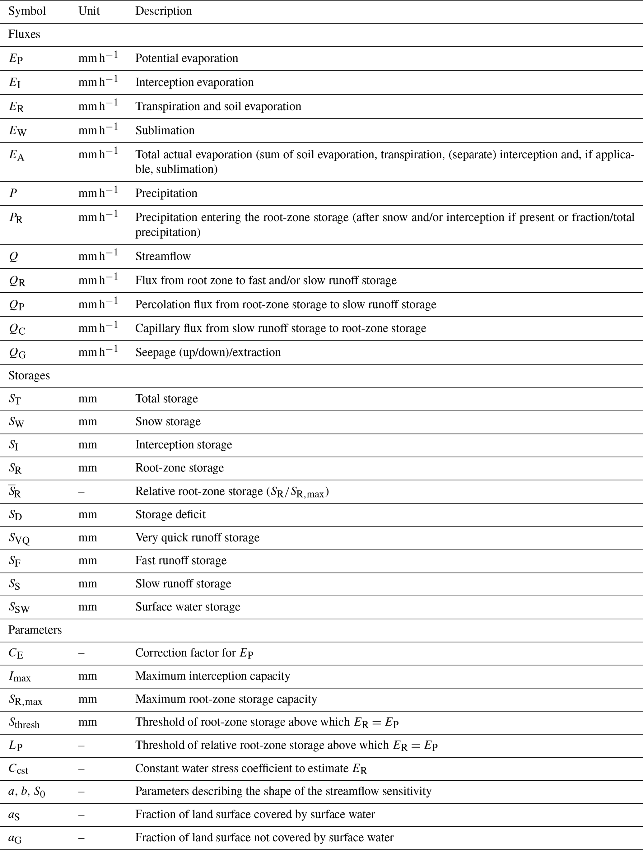
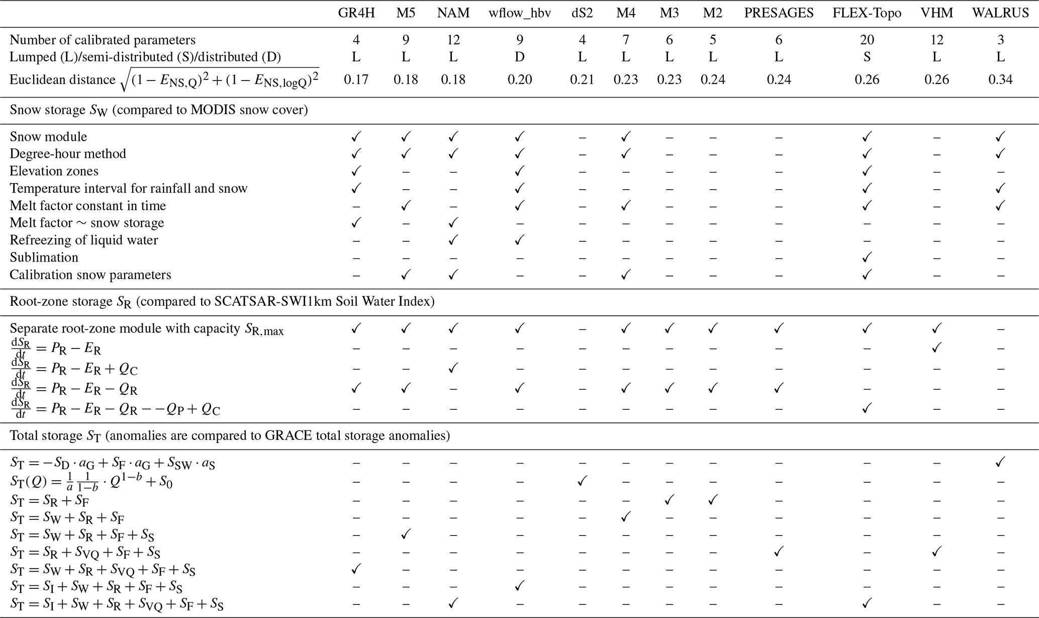
Table 2Number of calibrated model parameters, spatial distribution, and model performance calculated for the period 2008–2017 with the Euclidean distance where a value of 0 would indicate a perfect model. Main characteristics describing snow storage, root-zone storage and total storage per model. Notations are defined in Table 1.
4.2 Model evaluation: water balance
All the models are evaluated in terms of the long-term water balance, which indicates the partitioning between drainage and evaporative fluxes and allows us to assess long-term conservation of water and energy. We compare mean annual streamflow with observations and mean annual actual evaporation and interception evaporation with GLEAM estimates for the Ourthe at Tabreux during the evaluation period 2008–2017. A detailed description of streamflow performance for specific events (low and high flows, snowmelt events, transition from dry to wet periods) has been detailed in the previous paper (de Boer-Euser et al., 2017). In the current study, differences in streamflow dynamics are briefly summarized by assessing observed and modeled baseflow indices (Ibaseflow, van Dijk, 2010) and flashiness indices (Iflashiness, Fenicia et al., 2016), as these are representative of the partitioning of drainage into fast and slow responses. Seasonal dynamics of actual evaporation over potential evaporation and runoff coefficients during winter (October–March) and summer (April–September) are compared between the models.
4.3 Model evaluation: internal states
We compare modeled snow storage, root-zone soil moisture and total storage between the models and with remote-sensing estimates of MODIS snow cover, SCATSAR-SWI1km Soil Water Index and GRACE total storage anomalies, respectively, as shown in Tables 2–3.
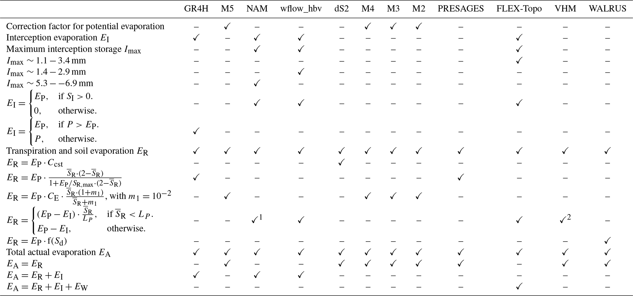
Table 3Main characteristics describing evaporation processes per model (where ✓1 indicates LP=1 and ✓2 indicates EI=0). Notations are defined in Table 1.
4.3.1 Snow days
As most models used in this study are lumped, it is not possible to spatially evaluate modeled snow cover versus MODIS snow cover. However, we can classify each day in a binary way according to the occurrence of snow, based on a threshold for the percentage of cells in the catchment where snow cover is detected. MODIS snow cover observations are classified as days with and without snow using thresholds of both 10 % and 15 % of snow-covered cells in the catchment to be counted as a day with snow, in a sensitivity analysis. For each model, snow days are distinguished from non-snow days whenever the water stored as snow is above 0.05 mm to account for numerical rounding. For each model (and each retained parameter set), we then compare whether modeled snow coincides with “truly” observed snow by MODIS, for each day with a valid MODIS observation. We create a confusion matrix with counts of true positives when observations and model results agree on the presence of snow (hits), false positives when the model indicates the presence of snow but this is not observed by MODIS (false alarms), false negatives when the model misses the presence of snow observed by MODIS (miss) and true negatives when observations and model results agree on the absence of snow (correct rejections). This allows us to identify the trade-off between, on the one hand, the miss rate between model and remote-sensing observation, as the ratio of misses over actual positives (number of days when snow is observed by MODIS) and, on the other hand, the false discovery rate as the ratio of false alarms over predicted positives (number of days when snow is modeled). We also compare annual maximum snow storage and number of days with snow between the seven models with a snow module (GR4H, M5, NAM, wflow_hbv, M4, FLEX-Topo, WALRUS). The snow analysis is performed in the catchment of the Ourthe Orientale upstream of Mabompré as it features the narrowest elevation range among the study catchments (i.e., 294–662 m a.s.l. versus 108–662 m for the Ourthe upstream of Tabreux) and thus plausibly permits a lumped representation of the snow component.
4.3.2 Root-zone soil moisture
We compare the range of the relative root-zone soil moisture (, Table 1) between the models for the period in which SCATSAR-SWI1km is available (2015–2017). Time series of catchment-scale root-zone soil moisture are available for all the models except WALRUS and dS2 as these models have a combined soil reservoir (Fig. 2). The dS2 model only relies on the sensitivity of streamflow to changes in total storage. In WALRUS, the state of the soil reservoir (which includes the root zone) is expressed as a storage deficit and is therefore not bound by an upper limit (Table 2). Root-zone storage capacities (SR,max, mm) are available as a calibration parameter for all the other models. We relate the range in relative root-zone soil moisture to the maximum root-zone storage capacity SR,max, because we expect models with small root-zone storage capacities SR,max to entirely utilize the available storage through complete drying and saturation.
We then compare the similarity of the dynamics of modeled time series of the relative root-zone soil moisture with the remotely sensed SCATSAR-SWI1km Soil Water Index for several values of the characteristic time length parameter (T in days). The T value has previously been positively correlated with root-zone storage capacity, assuming a high temporal variability of root-zone soil moisture and therefore a low T value for small root-zone storage capacities SR,max (Bouaziz et al., 2020). For each model and feasible realization, we identify the T value that yields the highest Spearman rank correlation between modeled root-zone soil moisture and Soil Water Index. We then relate the optimal T value to the root-zone storage capacity SR,max. This analysis enables us to identify potential differences in the representation and the dynamics of root-zone storage between the models.
4.3.3 Total storage anomalies
For each model, we calculate time series of total storage (Table 2) and mean monthly total storage anomalies relative to the 2004–2009 time-mean baseline for comparison with GRACE estimates for the Ourthe upstream of Tabreux (ID1) and the Semois upstream of Membre-Pont (ID3). Both catchments coincide with two neighboring GRACE cells, allowing us to test how well the models reproduce the observed spatial variability. We further relate the modeled range of total storage (maximum minus minimum total storage over the time series) to Spearman rank correlation coefficients between modeled and GRACE estimates of total storage anomalies.
4.4 Interactions between storage and fluxes during dry periods
The impact of a relatively large (> 200 mm) versus relatively small (< 150 mm) root-zone storage capacity on actual evaporation, streamflow and total storage is assessed during a dry period in September 2016 by selecting two representative models with high streamflow model performance (GR4H and M5). The plausibility of the hydrological response of these two model representations is evaluated against remote-sensing estimates of root-zone soil moisture and actual evaporation.
4.5 Plausibility of process representations
The models are subsequently ranked and evaluated in terms of their consistency with observed streamflow, remote-sensing data and expert knowledge with due consideration of the uncertainty in the evaluation data, as detailed in Sect. 3.3. We summarize our main findings by evaluating the models in terms of their deviations around median annual streamflow, flashiness and baseflow indices, median annual actual evaporation and interception compared to GLEAM estimates, the number of days with snow over valid MODIS observations, the number of days per year with empty root-zone storage and the very dry total storage anomalies compared to GRACE estimates.
5.1 Water balance
5.1.1 Streamflow
All the models show high Nash–Sutcliffe efficiencies of the streamflow and the logarithm of the streamflow (ENS,Q and ENS,logQ) with median values of above 0.7 for the post-calibration evaluation period 2008–2017 (Fig. 3a and Table 2 for the calculation of the Euclidean distances). The interannual variability of streamflow agrees strongly with observations for each model in the period 2008–2017 (Fig. 3b). The difference between modeled and observed median streamflow varies between −5.6 % and 5.6 %, and the difference in total range varies between −9.6 % and 20 %. This is in line with our results in the previous paper, in which we also showed that all the models perform well in terms of commonly used metrics (de Boer-Euser et al., 2017). However, there are differences in the partitioning of fast and slow runoff, as shown by the flashiness and baseflow indices (Iflashiness and Ibaseflow) in Fig. 3c. The largest underestimation of the flashiness index occurs for M2 and dS2 (∼ 20 %), while FLEX-Topo shows the highest overestimation (26 %). FLEX-Topo and WALRUS underestimate the baseflow index most (41 % and 70 %, respectively), while GR4H and M5 show the highest overestimation (15 % and 21 %, respectively). There is a strong similarity between modeled and observed hydrographs for one of the best performing models M5, as quantified by its low Euclidean distance (Fig. 3d and Table 2). The GR4H model is the only one which includes deep groundwater losses, but they are very limited and represent only 1.6 % of total modeled streamflow of the Ourthe at Tabreux, or approximately 7 mm yr−1.
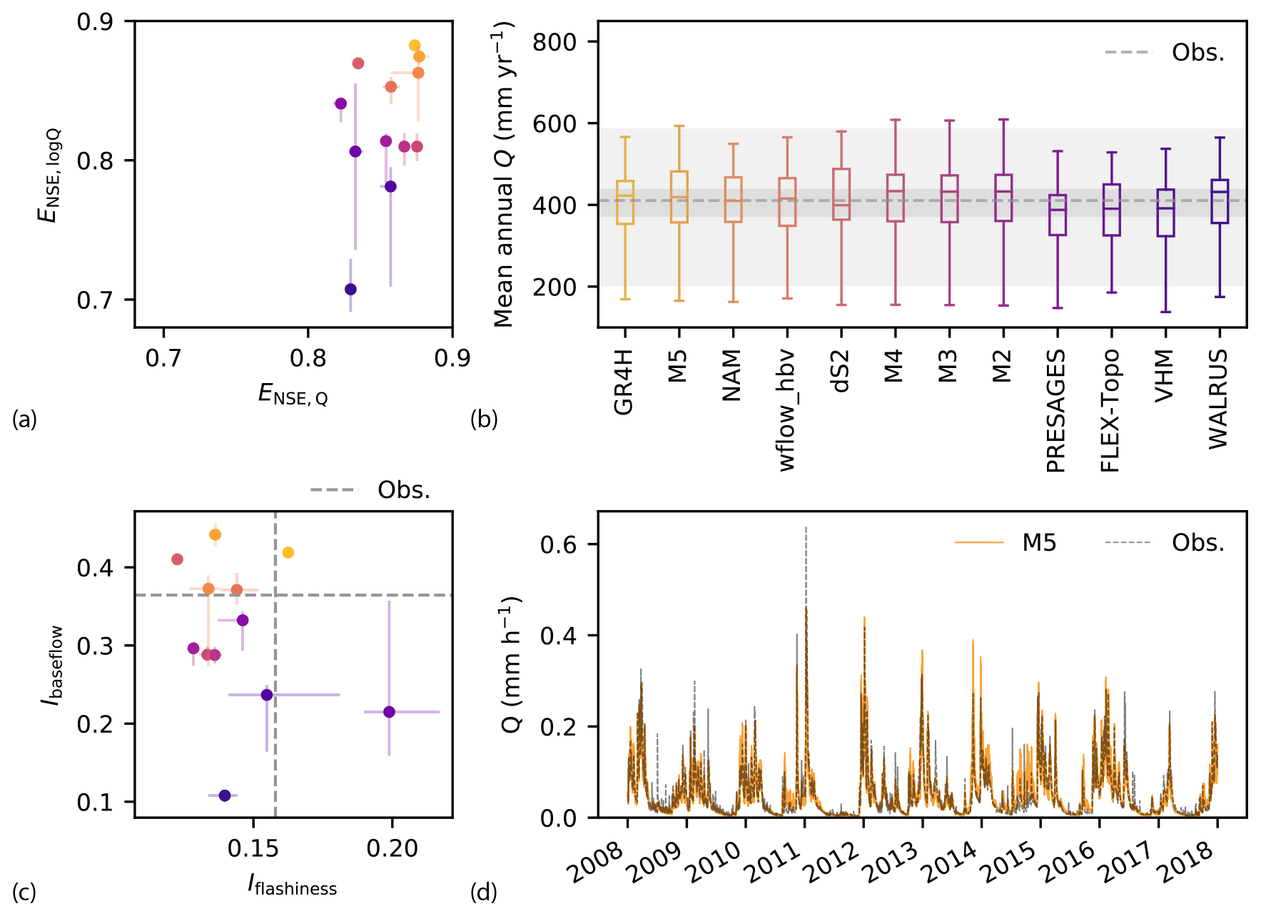
Figure 3Evaluation of modeled streamflow performance for the Ourthe at Tabreux for the period 2008–2017. (a) Nash–Sutcliffe efficiencies of the streamflow ENS,Q and the logarithm of the streamflow ENS,logQ (median, 25th/75th percentiles across parameter sets). (b) Modeled mean annual streamflow for hydrological years between 2008 and 2017 across feasible parameter sets. The models are ranked from the highest to the lowest performance according to the Euclidean distance of streamflow performance (see Table 2). The dashed line and grey shaded areas show median, 25th/75th and minimum–maximum range of observed mean annual streamflow. (c) Baseflow index Ibaseflow as a function of the flashiness index Iflashiness (median, 25th/75th percentiles across parameter sets). Observed values are shown by the grey dashed lines. (d) Observed and modeled hydrographs of model M5 with high streamflow model performance (low Euclidean distance).
5.1.2 Actual evaporation
Modeled median annual actual evaporation EA (computed as the sum of soil evaporation, transpiration, (separate) interception evaporation and, if applicable, sublimation, Table 3) for hydrological years between October 2008 and September 2017 varies between 507 and 707 mm yr−1 across models, with a median of 522 mm yr−1, which is approximately 10 % lower than the GLEAM estimate of 578 mm yr−1, as shown in Fig. 4a. Annual actual evaporation of the VHM model is very high compared to the other models, with a median of 707 mm yr−1, and approximates potential evaporation (median of 732 mm yr−1). Calibration of the VHM model is meant to follow a manual stepwise procedure including the closure of the water balance during the identification of soil moisture processes (Willems, 2014). However, in the automatic calibration prescribed by the current protocol, this step was not performed, which explains the unusual high actual evaporation in spite of relatively similar annual streamflow compared to the other models, as there is no closure of the water balance (Fig. 3a).
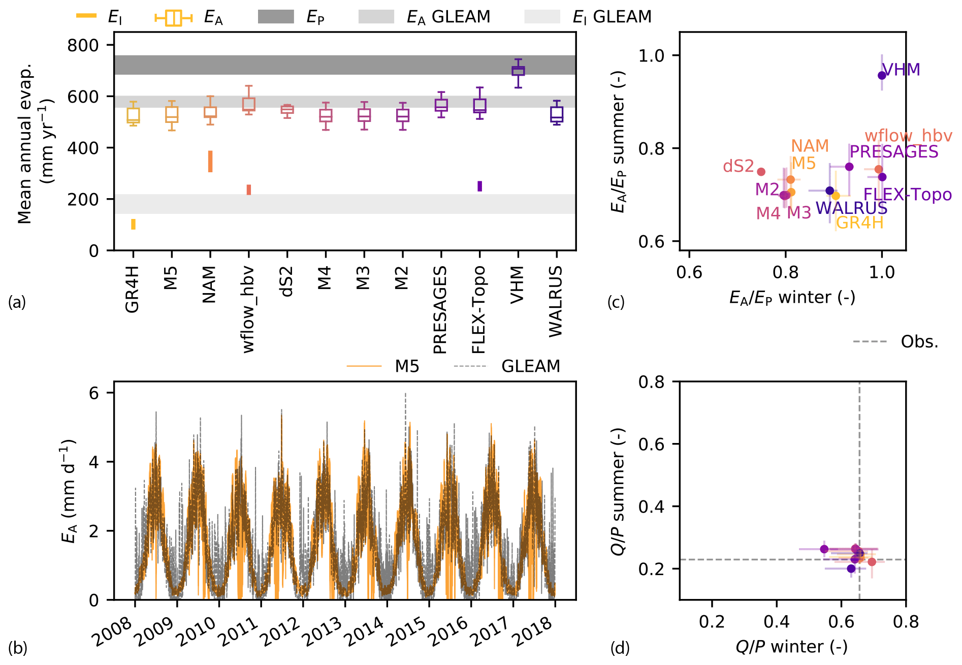
Figure 4Evaluation of modeled evaporation for the Ourthe upstream of Tabreux for the period 2008–2017. (a) Modeled mean annual actual evaporation EA and minimum–maximum range of mean annual interception evaporation EI for hydrological years between 2008 and 2017 across feasible parameter sets. The dark grey shaded area shows the range of potential evaporation EP used as input for the models. The light grey shaded area shows GLEAM actual and interception evaporation. (b) Daily actual evaporation from GLEAM and modeled by the M5 model. (c) Summer against winter EA/EP ratios for each model (median and 25th/75th percentiles across parameter sets). (d) Summer against winter runoff coefficient for each model (median and 25th/75th percentiles across parameter sets), plotted on the same scale. The dashed grey lines indicate the observed median runoff coefficients in summer and winter.
Interception evaporation is included in four models, with GR4H showing the lowest annual interception evaporation of 100 mm yr−1 (19 % of EA or 10 % of P), FLEX-Topo and wflow_hbv having relatively similar amounts of approximatively 250 mm yr−1 (∼ 45 % of EA or 26 % of P) and NAM having the highest annual interception evaporation of 340 mm yr−1 (65 % of EA or 36 % of P), as shown in Fig. 4a. Differences are related to the presence and maximum size of the interception storage (Imax), as shown in Table 3. GLEAM interception estimates of 189 mm yr−1 are almost twice as high as GR4H estimates, 25 % lower than FLEX-Topo and wflow_hbv, and 44 % lower than NAM values, suggesting a large uncertainty in the contribution of interception and transpiration to actual evaporation. For comparison, measurements of the fraction of interception evaporation over precipitation in forested areas vary significantly depending on the site location, with estimates of 37 % for a Douglas fir stand in the Netherlands (Cisneros Vaca et al., 2018), 27 %, 32 % and 42 % for three coniferous forests of Great Britain (Gash et al., 1980) and 50 % for a forest in Puerto Rico (Schellekens et al., 1999), and are difficult to extrapolate to other catchments due to the heterogeneity and complexity of natural systems.
GLEAM estimates of actual evaporation show relatively high evaporation rates in winter and are never reduced to zero in summer, as opposed to modeled M5 estimates, as shown in Fig. 4b. GLEAM actual evaporation minus the separately calculated interception is 94 % of potential evaporation, implying almost no water-limited conditions, as opposed to our models in which actual evaporation in summer (April–September) is, due to water stress, reduced to approximately 73 % of potential evaporation on average for all the models except VHM (Fig. 4c). Larger differences between the models occur in the ratio during winter (October–March), when FLEX-Topo, wflow_hbv and VHM show ratios close to unity and dS2 the lowest values of 0.75 as shown in Fig. 4c. The dS2 model differs from all the other models as it relies on a year-round constant water stress coefficient (Ccst), independent of water supply, while the stress coefficient depends on root-zone soil moisture content in all the other models (Table 3).
Most models slightly overestimate summer runoff coefficients, with values between 0.22 and 0.26, which are very close to the observed value of 0.22, as shown in Fig. 4d. During winter, runoff coefficients vary between 0.55 and 0.71, which is close to the observed value of 0.66. This implies a relatively high level of agreement between the models in reproducing the medium- to long-term partitioning of precipitation into evaporation and drainage and thus in approximating at least long-term conservation of energy (Hrachowitz and Clark, 2017).
5.2 Internal model states
5.2.1 Snow days
MODIS snow cover is detected over most of the catchment area for some time each year between November 2001 and November 2017, except for the periods of November 2006 to March 2007 and November 2007 to March 2008, when snow is detected in less than half of the catchment cells, as shown in Fig. 5a. The number and magnitude of modeled snow storage events varies between the models (Fig. 5b). The modeled number of snow days per hydrological year varies from ∼ 28 d for FLEX-Topo, WALRUS and wflow_hbv to ∼ 62 d for GR4H and ∼ 90 d for NAM, M4 and M5, as shown in Fig. 5c. The variability in median annual maximum snow storage varies from 3 mm for wflow_hbv and ∼ 5–6 mm for FLEX-Topo and WALRUS to ∼ 10 mm for GR4H, M4, and M5 and 15 mm for NAM. We further evaluate the plausibility of these modeled snow processes by comparing modeled and observed snow cover for days when a valid MODIS observation is available.
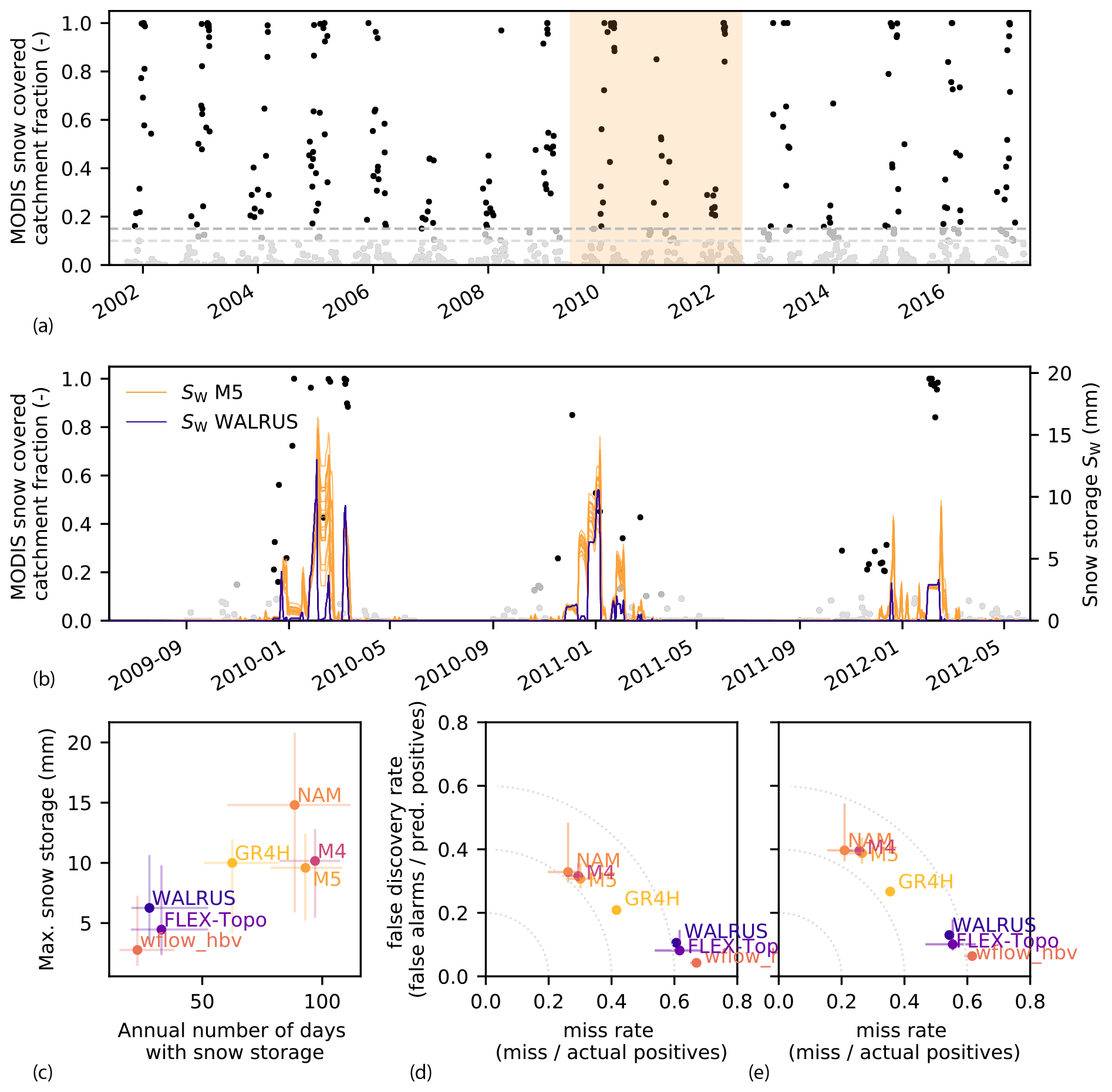
Figure 5(a) Fraction of cells with a MODIS areal fraction snow cover greater than zero in the Ourthe Orientale upstream of Mabompré for the period 2001–2017. MODIS data are available once every 3 d on average. The dashed lines show the two thresholds of 10 % and 15 % selected to distinguish snow days. (b) Modeled snow storage for two contrasting models M5 and WALRUS for the light orange shaded period. (c) Median annual maximum snow storage as a function of number of days per year with snow. Light (yellowish) colors indicate models with higher performance (lower Euclidean distances). The vertical and horizontal error bars indicate the 25th/75th percentiles over time and feasible parameter sets. (d, e) Two-dimensional representation of the false discovery rate as a function of the miss rate when applying thresholds of (d) 10 % and (e) 15 % of cells within the catchment with snow cover greater than zero. In this representation, the perfect model would be at the origin (0 % misses and 0 % false alarms). The dotted lines show the distance from the origin. The vertical and horizontal error bars indicate the uncertainty within feasible parameter sets.
The presence of snow modeled by FLEX-Topo, wflow_hbv and WALRUS coincides for 92 % with the presence of snow observed by MODIS. However, these models fail to model snow for ∼ 62 % of days when MODIS reports the presence of snow, implying that these models miss many observed snow days, but when they predict snow, it was also observed (Fig. 5d).
NAM, M4 and M5, on the other hand, predict the presence of snow which coincides with snow observed by MODIS in ∼ 68 % of the positive predictions, implying a relatively high probability of false alarm snow prediction of ∼ 32 %. However, they miss only ∼ 29 % of actual positive snow days observed by MODIS (Fig. 5d). This suggests that these models miss fewer observed snow days, but they also overpredict snow day numbers, which could be related to the use of a single temperature threshold to distinguish between snow and rain, as opposed to a temperature interval in the other models (Table 2).
GR4H is in between the two previously mentioned model categories, with a snow prediction which coincides with observed snow by MODIS in 79 % of the positive predictions and therefore only 21 % of false alarms. The model misses 42 % of actual positive snow days observed by MODIS. GR4H therefore shows a more balanced trade-off between the number of false alarms and the number of observed snow events missed. This is illustrated in Fig. 5d.
With an increased threshold to distinguish snow days in MODIS, from 10 % to 15 % of cells in the catchment with a detected snow cover (Fig. 5d and e, respectively), we decrease the number of observed snow days. For all the models, this leads to an increase in the ratio of false alarms over predicted snow days but also a decrease in the ratio of missed events over actual snow days observed by MODIS. However, as all the models are similarly affected by the change in threshold, our findings on the differences in performance between the models show little sensitivity to this threshold.
Despite the large variability in snow response between the models, snow processes are represented by a degree-hour method in all the models, suggesting a high sensitivity of the snow response to the snow process parameterization (Table 2).
5.2.2 Root-zone soil moisture
Vegetation-accessible water volumes that can be stored in the root zone largely control the long-term partitioning of precipitation into evaporation and drainage. Most hydrological models include a representation of this root-zone storage capacity SR,max, which is estimated through calibration (Table 2). The calibrated root-zone storage capacities vary between 74 and 277 mm across studied models. The root-zone soil moisture content relative to saturation of models with relatively large root-zone storage capacities (here defined as 200 mm) tends to never fully dry out (> 0.20) and saturate (< 0.94) as opposed to models with lower root-zone storage capacities ( 150 mm), in which the storage tends to either dry out completely and/or fully saturate (Fig. 6a). If the vegetation-accessible water storage dries out, this will lead to water stress and reduced transpiration. On the other hand, if the root-zone storage is saturated, no more water can be stored, resulting in fast drainage. The size of the root-zone storage capacity is therefore a key control of the hydrological response, allowing us to explain some of the observed variability between the models.
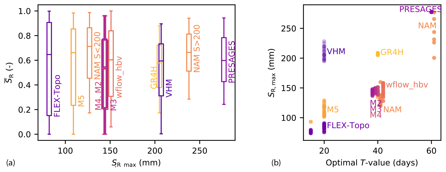
Figure 6(a) Range of relative root-zone soil moisture in the Ourthe upstream of Tabreux for the period 2015–2017 as a function of the median root-zone storage capacity (SR,max) across parameter sets. The feasible parameters for NAM are split into two groups due to the large variability of SR,max (subsets with SR,max of ∼ 130 and ∼ 240 mm). (b) Root-zone storage capacity SR,max as a function of the optimal T value for each model realization. Optimal T values are derived at the highest Spearman rank correlation between the Soil Water Index and modeled root-zone soil moisture.
We compare the dynamics of modeled and remote-sensing estimates of root-zone soil moisture by calculating Spearman rank correlations between modeled root-zone soil moisture and remote-sensing estimates of the Soil Water Index for the available T values of 2, 5, 15, 20, 40, 60 and 100 d. As the T value increases, the Soil Water Index is more smoothed and delayed. For each model realization, we identify the T value which yields the highest Spearman rank correlation between Soil Water Index and modeled root-zone soil moisture (Fig. 6b). The optimal T value increases with the size of the calibrated root-zone storage capacity and varies between 15 and 60 d. A small root-zone storage capacity is indeed likely to fill through precipitation and empty through evaporation and drainage more rapidly than a large water storage capacity, leading to a higher temporal relative soil moisture variability. The mismatch between the relatively high root-zone storage capacities of VHM ( 200 mm) in relation to the relatively low optimal T values of 20 d is likely related to the unclosed water balance (Sect. 5.1.2). The similarity between modeled root-zone soil moisture and Soil Water Index with optimal T values is high, as implied by Spearman rank correlations varying between 0.88 and 0.90 across models. However, the disparity in optimal T values between the models underlines the different temporal representations of root-zone soil moisture content across models, implying that all these models cannot simultaneously provide a plausible representation of the catchment-scale vegetation-accessible water content.
5.2.3 Total storage anomalies
Total water storage anomalies obtained from GRACE are compared to the storage as simulated by the models, showing relatively similar seasonal patterns, as illustrated in Fig. 7a for model M5. GRACE total storage anomalies of the Semois upstream of Membre-Pont and the Ourthe upstream of Tabreux are mainly represented by two neighboring cells (Fig. 1b), allowing us to test how models represent the observed spatial variability. The range of anomalies in the Semois upstream of Membre-Pont is larger than in the Ourthe upstream of Tabreux, implying 18 %, 3 % and 7 % less summer and 19 %, 19 % and 10 % more winter storage in the Semois upstream of Membre-Pont for each of the three GRACE processing centers (Fig. 7b). Median precipitation is also 37 % higher in the Semois upstream of Membre-Pont than in the Ourthe upstream of Tabreux during winter months (October–March) but relatively similar during summer months (April–September). This difference in precipitation potentially leads to a wider range of modeled anomalies in the Semois upstream of Membre-Pont than in the Ourthe upstream of Tabreux for all the models, as shown in Fig. 7c. This implies that all the models reproduce the spatial variability between both catchments observed by GRACE. As the models were calibrated for the Ourthe at Tabreux and parameter sets were transferred to the Semois upstream of Membre-Pont, the forcing data are the main difference for explaining the modeled spatial variability.
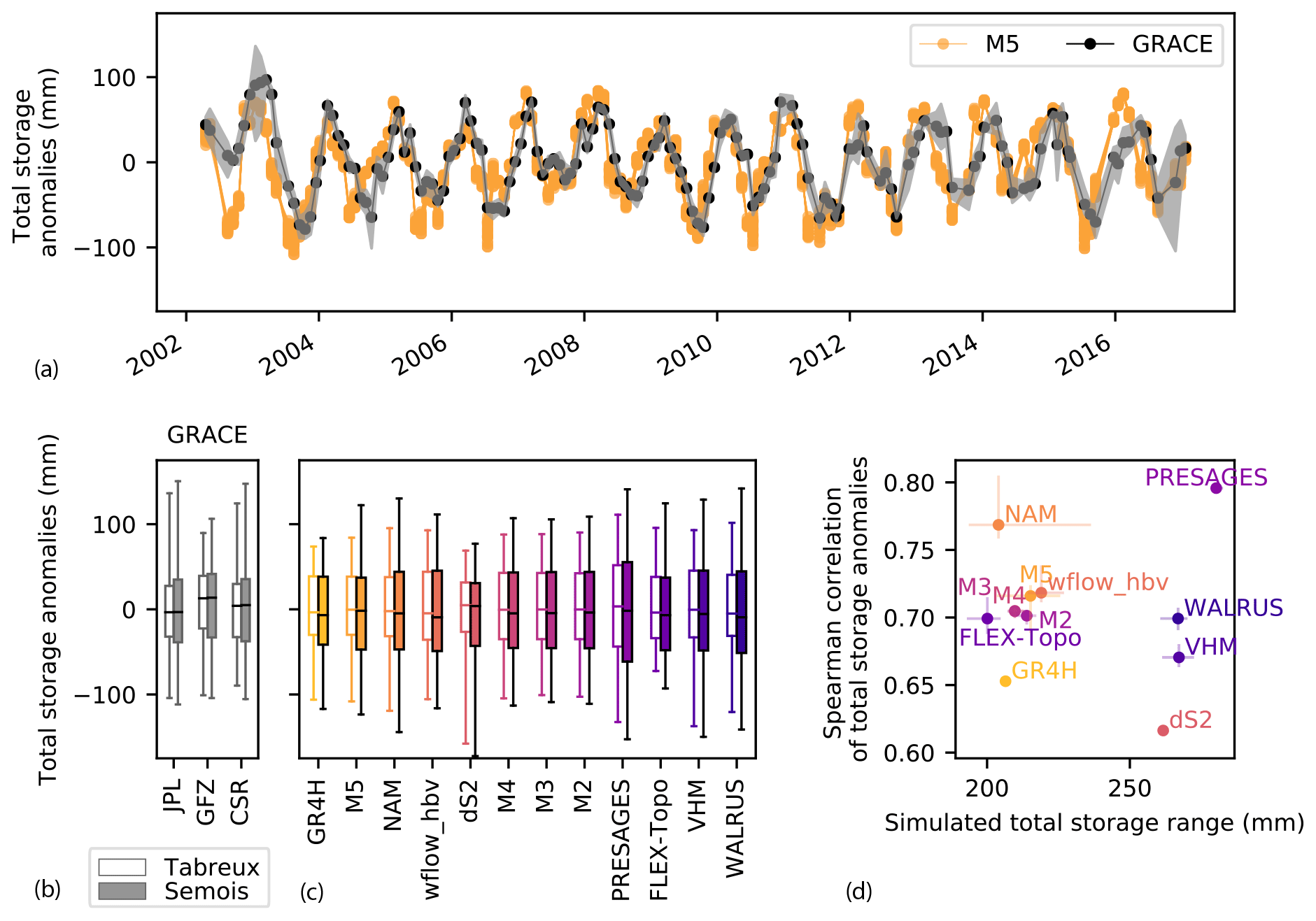
Figure 7(a) Total storage anomalies modeled by M5 and compared to GRACE for the Ourthe upstream of Tabreux. The grey band shows the variability in total storage anomalies of the three processing centers. (b) Range of GRACE total storage anomalies for the three processing centers for the Semois upstream of Membre-Pont compared to the Ourthe upstream of Tabreux for the period 2001–2017. (c) Modeled total storage anomalies for both catchments. (d) Spearman rank correlations between GRACE and modeled total storage anomalies as a function of the range of modeled total storage for the Ourthe upstream of Tabreux.
The models are also able to represent the observed temporal dynamics of total storage anomalies, as suggested by Spearman rank correlation coefficients ranging between 0.62 and 0.80 for the Ourthe upstream of Tabreux (Fig. 7d). There is, however, no relation between the Spearman rank correlations of the anomalies and the total modeled storage range (difference between maximum and minimum values), as shown in Fig. 7d. PRESAGES, WALRUS, VHM and dS2 have the largest ranges of total modeled storage, varying between 260 and 280 mm, and are also characterized by relatively large root-zone storage capacities (PRESAGES and VHM) or no separate root zone (WALRUS and dS2), while the total storage range of all the other models is between 200 and 220 mm. The similarity in total storage range between most models is likely related to the identical forcing data and the similarity in the long-term partitioning of precipitation into drainage and evaporation (Sect. 5.1.2). However, the absolute values of total storage during a specific event or the partitioning into internal storage components may vary between the models (Sect. 5.3).
5.3 Interactions between storage and fluxes during dry periods
As previously seen in Fig. 6a, the relative root-zone soil moisture content of the GR4H model is always above 0.2 for the 3 years for which SCATSAR-SWI1km data are available, as opposed to M5, which fully dries out for some time during the summers of 2015–2017. The Normalized Difference Vegetation Index of MODIS (NDVI, Didan, 2015a, b) also does not show a sharp decrease during these periods (Fig. 8a, b). Actual evaporation in M5 is strongly reduced during these dry soil moisture periods, unlike GR4H, as shown in Fig. 8c, d. When zooming into the dry period around September 2016, Fig. 8e, f show median relative root-zone soil moisture in GR4H of ∼ 0.24 versus ∼ 0.01 for M5, while SCATSAR-SWI1km has a higher median value of ∼ 0.55 (for both optimal T values of 20 and 40 d). The dryness of root-zone soil moisture in M5 leads to median daily evaporation of 0.8 against 1.3 mm d−1 for GR4H and prolonged periods of almost-zero evaporation in M5 (e.g., 31 August –3 September, 9–15 September and 22–30 September), while this neither occurs in GR4H nor in GLEAM actual evaporation, as shown in Fig. 8g, h. Despite the high streamflow performance of model M5 (Fig. 3, Table 2), it is unlikely that transpiration is reduced to almost zero for several days in a row each summer in a catchment where approximately half of the area is covered by forests. This is also not supported by the remote-sensing data of soil moisture, NDVI and evaporation. High streamflow performances, therefore, do not warrant the plausibility of internal process representation. Despite the dried-out root-zone storage in M5, there is still water available in the slow storage to sustain a baseflow close to observed values, as shown in Fig. 8j, l. The streamflow responses of GR4H and M5 are both close to observations (Fig. 8i, j) in spite of differences in storage and evaporation, suggesting different internal process representations for a similar aggregated streamflow response during a low-flow period.
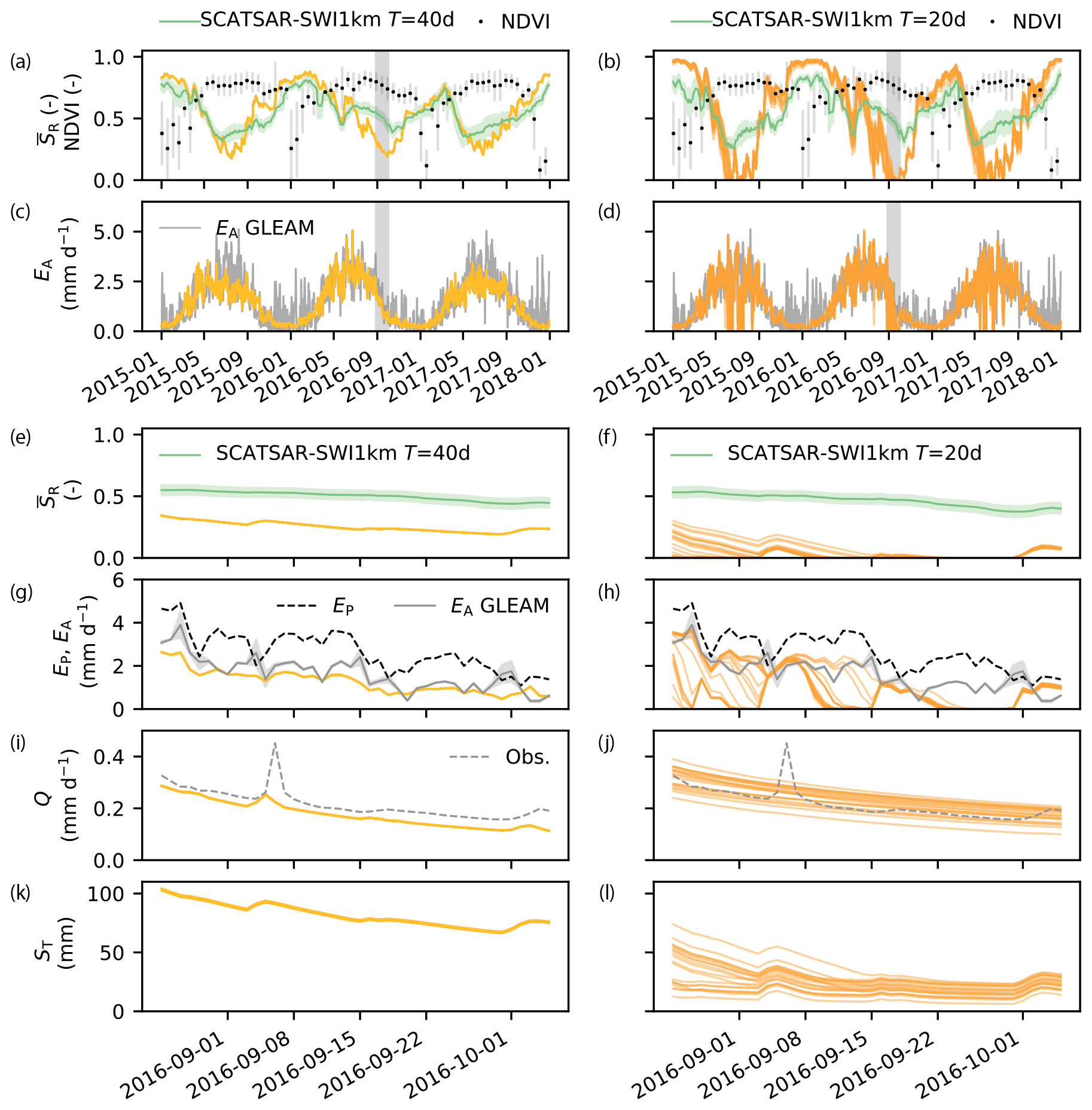
Figure 8(a,b) Modeled relative root-zone soil moisture , SCATSAR-SWI1km Soil Water Index with optimal T value and NDVI for the period 2015–2017 for GR4H (yellow) and M5 (orange), respectively. The error bars and bands show the standard deviation of the remote-sensing data within the catchment area. (c, d) Actual evaporation EA by GR4H and M5 for the period 2015–2017, showing a large reduction of evaporation during summer for M5, unlike GR4H and GLEAM actual evaporation. (e, f) Zoomed-in modeled and SCATSAR-SWI1km root-zone soil moisture for the grey shaded period of September 2016 in (a), (b), (c), and (d). (g, h) Potential, modeled and GLEAM actual evaporation, (i, j) modeled and observed streamflow Q, and (k, l) total storage ST for the September 2016 dry period. The narrow uncertainty band of the GR4H model is related to its converging parameter search method.
5.4 Plausibility of process representations
The models are ranked and evaluated for a selection of criteria using observed streamflow, remote-sensing data and expert knowledge (Figs. 9 and S3 in the Supplement). All the models deviate less than ±6 % from observed median annual streamflow (Fig. 9a), which is less than the estimated uncertainty of 11 % (Sect. 3.3). In contrast, the modeled flashiness and baseflow indices of most models deviate more than the estimated uncertainty (Fig. 9b, c). FLEX-Topo is the only model with a clear overestimation of the flashiness index, which relates to the calibration aim of having a flashy model to reproduce small summer peaks (de Boer-Euser et al., 2017).
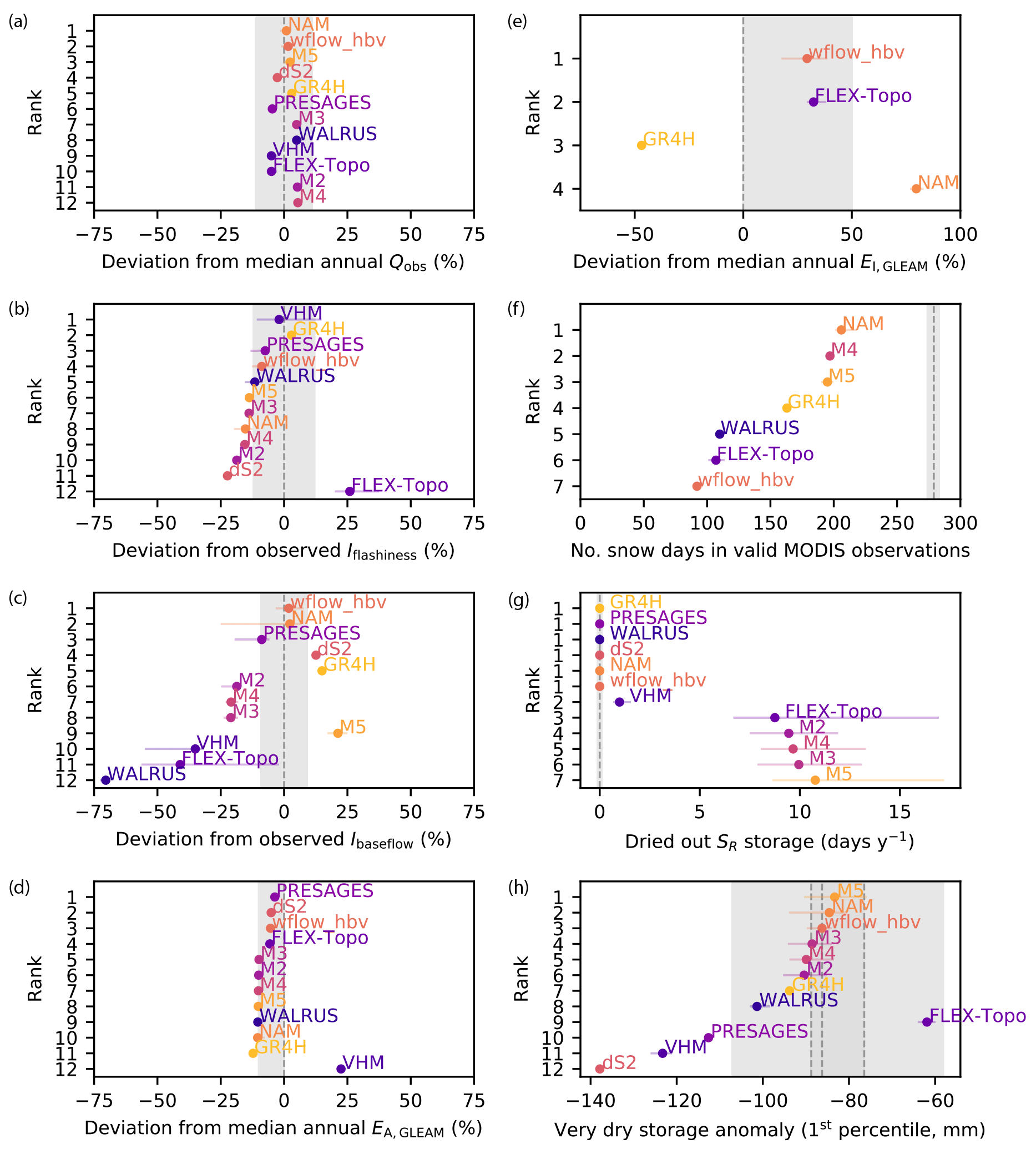
Figure 9Ranking and evaluation of model behavior for a selection of criteria based on observed streamflow, remote-sensing data and expert knowledge. The grey shaded areas are soft indications of more plausible behavior based on uncertainty estimates and expert knowledge. Model ranks as a function of the (a) deviation from observed median annual streamflow; (b) deviation from the flashiness index; (c) deviation from the baseflow index; (d) deviation from median annual GLEAM actual evaporation; (e) deviation from median annual GLEAM interception for models with a separate interception module; (f) number of days with snow cover for valid MODIS observations between 2001 and 2017 for models with a snow module; (g) annual number of days when the root-zone storage is dry (filled with less than 1 % of its capacity); (h) deviation from the 1st percentile of GRACE total storage anomalies for the three centers. The error bars show the 25th–75th range across the ensemble of feasible parameter sets. Results are for the Ourthe catchment upstream of Tabreux, except for the snow analysis.
Modeled median annual total actual evaporation deviates by approximately −10 % from GLEAM estimates, except for the +22 % overestimation of the VHM model due to the issue of the unclosed water balance, as shown in Fig. 9d. These results are consistent with the evaluation study of GLEAM compared to other evaporation products (Miralles et al., 2016), which reports higher than average values for GLEAM in Europe (∼ +10 % at our latitude).
Four models explicitly account for interception with a separate module. Median annual interception rates deviate substantially from GLEAM estimates (−47 % to +80 %) as shown in Fig. 9e. There is a high uncertainty in the partitioning of evaporation into different components in evaporation products, and GLEAM likely underestimates interception rates (Miralles et al., 2016; Zhong et al., 2020). Therefore, we consider a large uncertainty of +50 % to evaluate and rank the models. The GR4H interception is lower than GLEAM estimates. However, an interception storage was recently included in an hourly GR model (GR5H) to better represent the interception processes (Ficchì et al., 2019; Thirel et al., 2020).
All the models substantially underestimate the number of days when snow is observed by MODIS at the catchment scale for all valid MODIS observations (cloud cover < 40 % and excluding summer months), as shown in Fig. 9f. Yet we estimate a low uncertainty of less than 2 % around this number (Sect. 3.3). The NAM, M4 and M5 models are closest to MODIS estimates, but they are characterized by high false alarm rates (Fig. 5d), which implies a mismatch in the modeled and observed days with snow for valid MODIS observations. Based on expert knowledge (Royal Meteorological Institute Belgium, 2015) and the trade-off between miss rate and false discovery rate (Fig. 5d, e), we expect the annual number of days with snow storage to be between 28 and 62 d yr−1 as modeled by wflow_hbv, WALRUS, FLEX-Topo and GR4H, whereas the ∼ 90 d yr−1 of NAM, M4 and M5 seems too high.
The FLEX-Topo and M2 to M5 models are characterized by an empty root-zone storage for approximately 10 d yr−1 ( < 1 %) as shown in Fig. 9g. These models have in common that evaporation from the root zone occurs at a potential rate and is not (or hardly) reduced when soils become dry until the point where the storage is empty. This is the case for models with a very low or no evaporation reduction parameter LP. This behavior is not supported by the remote-sensing data of evaporation, soil moisture and NDVI (Sect. 5.3) nor by theory on root water uptake reduction under dry conditions (Feddes, 1982). The additional slow groundwater reservoir added in model M5 compared to M2–M4 leads to a smaller root-zone storage capacity as the available storage is partitioned into the root-zone storage and the additional groundwater store. The smaller root-zone storage capacity of model M5 exacerbates the number of annual days with empty storage. This highlights the complex interactions in internal dynamics even in parsimonious lumped models with similar mean annual streamflow performance.
Catchments with relatively large root-zone storage capacities underestimate GRACE estimates of very dry storage anomalies most (Figs. 6 and 9h). The uncertainty of GRACE is represented by the estimates of the three processing centers and the ∼ 18 mm uncertainty estimate mentioned in Sect. 3.3. FLEX-Topo has a low root-zone storage capacity and is the only model which overestimates the very dry storage anomalies. Models with root-zone storage capacities of around 110 to 150 mm show the most consistent behavior with GRACE estimates of very dry storage anomalies.
While streamflow alone may be used to evaluate hydrological models, we subsequently use these models to understand internal states and fluxes in current and future conditions (Alcamo et al., 2003; Hagemann et al., 2013; Beck et al., 2017) or to make operational streamflow predictions (e.g., HBV and GR types of models are used by the Dutch and French forecasting services). Our findings show that similar streamflow responses obtained by models calibrated according to an identical protocol rely on different internal process representations. While not unexpected, it implies that we might get the right answers but for the wrong reasons (Kirchner, 2006), as these models cannot at the same time all be right and different from each other (Beven, 2006).
Almost all the models show a similar long-term partitioning of precipitation into drainage and evaporation, as they are forced and constrained by the same data, also leading to relatively similar volumes of total storage. However, the partitioning of total storage into several internal storage components differs between the models, resulting in distinct runoff responses as expressed by the baseflow and flashiness indices.
None of the models is systematically consistent with the information available from streamflow observations, remote-sensing data and expert knowledge. However, some processes either play a limited role in the overall water balance or can be compensated by other processes. Snow occurs every year but is not a major component of the streamflow regime (de Wit et al., 2007), interception evaporation can be compensated by root-zone evaporation, and very dry periods only occur for several weeks per year when streamflow is already very low. There is also a large uncertainty in each of the data sources, which makes us reluctant to use them to determine hard thresholds to reject models. Instead, we ranked the models for a selection of “soft” criteria and found that NAM, wflow_hbv and PRESAGES are overall most consistent with the evaluation data, with median ranks of 2–3 (Fig. S3 in the Supplement). While an overall ranking may be useful for practitioners, modelers benefit more from the specific ranking for each criterion to detect specific model deficiencies that could be improved in the model structure. An overall ranking is only a mere indication which should be interpreted carefully due to uncertainty in the evaluation data and the applied calibration strategy.
The presence of interception or a slow storage (absent in M2–M4 but added in M5) affects the representation of other internal processes, including transpiration and/or root-zone soil moisture, implying that individual internal model components are altered by the presence/absence of other potentially compensating processes. Adding an additional internal model component changes the internal representation of water storage and fluxes through the system, which should be kept in mind if model parameters were to be fixed in alternative model structures. Furthermore, model improvements through additional process components and/or adapted parameterization should be evaluated in terms not only of the aggregated response, but also the partitioning of fluxes and storages through the system (e.g., does the groundwater component improve the baseflow index at the expense of the availability of root-zone soil moisture during dry periods?). Models should be confronted with expert knowledge, e.g., on the occurrence of days with water stress or snow storage, to assess the plausibility of internal states and fluxes (Gharari et al., 2014; Hrachowitz et al., 2014; van Emmerik et al., 2015).
Applying these models to a future, more extreme climate in the same region might lead to contrasting insights regarding impacts of climate change, as also shown by studies of Hagemann et al. (2013), Melsen et al. (2018) and de Niel et al. (2019), in which model structures may lead to different signs of change in mean streamflow. Using one model or the other to assess the effect of rising temperatures on snow could lead to very different timescales of snow storage decline. Vegetation already experiences more intense water stress in some models compared to others, and this would be exacerbated in more extreme drought scenarios (Melsen and Guse, 2019). More intense precipitation events could affect interception evaporation and therefore water availability in the root zone differently from one model to another. Beyond model structure, the experience each modeler has with their model and associated calibration procedure to constrain model parameters may also impact the simulation results (Melsen et al., 2019).
Our findings should, therefore, encourage modelers to use multiple data sources for model calibration and evaluation, as already suggested by many other studies (Samaniego et al., 2010; Rakovec et al., 2016a; Koch et al., 2018; Stisen et al., 2018; Nijzink et al., 2018; Veldkamp et al., 2018; Dembélé et al., 2020). Remote-sensing estimates of soil moisture, evaporation and total storage anomalies are available at the global scale, and in spite of potential biases with models, the temporal dynamics are useful for constraining our models (McCabe et al., 2017; Sheffield et al., 2018). Additionally, it seems essential to support decision-makers by studies relying on multi-model and multi-parameter systems, as also suggested by Haddeland et al. (2011) and Schewe et al. (2014), to reveal uncertainties inherent to the heterogeneous hydrological world (Beven, 2006; Savenije, 2010; Samaniego et al., 2010; Hrachowitz and Clark, 2017).
This study is the result of a joint research effort of scientists and practitioners gathering each year in Liège at the International Meuse Symposium to exchange interdisciplinary and intersectoral knowledge related to the Meuse basin. Although coordination of large international teams may be challenging, international studies favor close collaboration between scientists and practitioners, who can learn from each other to accelerate modeling advances (Archfield et al., 2015). Another advantage of comparing modeling results of several research groups is to quickly detect small mistakes in the modeling process, including shifts in the time series or using forcing data of one catchment to model another catchment. While hydrograph characteristics were the main focus of the previous study (de Boer-Euser et al., 2017), we gain distinct insights into the plausibility of model behavior by evaluating additional facets of internal process representation using remote-sensing data.
Many aspects of the hydrological response remain unknown and can hardly be evaluated against observations. While in situ observations of snow, evaporation or soil moisture are rarely available at a sufficient spatio-temporal scale, remote-sensing estimates have the advantage of high spatial resolution and worldwide spatial coverage, though they often rely on models themselves and are affected by high and often unknown uncertainty. Comparing models with these independent observations is valuable for evaluating their consistency and detecting outliers. However, these observations cannot be considered representative of the truth as they rely on many assumptions themselves, hindering “real” hypothesis testing. The ratio of actual over potential evaporation as a result of water stress at the catchment scale, therefore, remains highly uncertain (Coenders-Gerrits et al., 2014; Mianabadi et al., 2019). While areal fractions of snow cover can be estimated by MODIS, the presence of clouds limits the usability of the data, and knowledge of the catchment-scale snow water equivalent is lacking. If remote-sensing estimates of near-surface relative soil moisture are available, root-zone water content remains uncertain, and while GRACE provides estimates of total storage anomalies, we lack knowledge on absolute total water storage. The spatial variability and the temporal dynamics of these remote-sensing products provide useful, additional, independent information to understand the hydrological puzzle but certainly not all the answers to evaluate the states typically included in process-based models. Measurements are, therefore, of crucial importance to increase our understanding of hydrological processes at the catchment scale, which in turn will improve the quality of remote-sensing products and model development (Vidon, 2015; Burt and McDonnell, 2015; van Emmerik et al., 2018).
The evaluation of model behavior is conditional on the calibration procedure, which was freely chosen by the individual contributing institutes. The use of different or more calibration objectives and in-depth uncertainty estimation (Beven and Binley, 1992) may have resulted in different conclusions in terms of the plausibility of the behavior of each model.
We performed a thorough analysis of 12 models, five variables and three catchments. We deliberately chose to limit the number of study catchments to balance depth with breadth, allowing us to dive into process-relevant insights.
Similar streamflow performance of process-based models, calibrated following an identical protocol, relies on different internal process representations. Most models are relatively similar in terms of the long-term partitioning of precipitation into drainage and evaporation. However, the partitioning between transpiration and interception, snow processes and the representation of root-zone soil moisture varies significantly between the models, suggesting variability of water storage and release through the catchment. The comparison of modeled states and fluxes with remote-sensing estimates of evaporation, root-zone soil moisture and vegetation indices suggests that models with relatively small root-zone storage capacities and without reduction in root water uptake during dry conditions lead to unrealistic drying-out of the root-zone storage and significant reduction of evaporative fluxes each summer. Expert knowledge in combination with remote-sensing data further allows us to “softly” evaluate the plausibility of model behavior by ranking them for a set of criteria. Even if none of the models is systematically consistent with the available data, we did not formally reject specific models due to the uncertainty in the evaluation data and their changing relevance for the studied catchments. The dissimilarity in internal process representations between the models implies that they are not necessarily providing the right answers for the right reasons, as they cannot simultaneously be close to reality and different from each other. While the consequences for streamflow may be limited for the historical data, the differences may exacerbate for more extreme conditions or climate change scenarios. Considering the uncertainty of process representation behind the scenes of streamflow performance and our lack of knowledge and observations on these internal processes, we invite modelers to evaluate their models using multiple variables, encourage more experimental research, and highlight the value of multi-model multi-parameter studies to support decision-making.
Streamflow and precipitation data were provided by the Service Public de Wallonie in Belgium (Direction générale opérationnelle de la Mobilité et des Voies hydrauliques, Département des Etudes et de l'Appui à la Gestion, Direction de la Gestion hydrologique intégrée (Bld du Nord 8-5000 Namur, Belgium)). Hourly radiation data were retrieved from the portal of the Royal Netherlands Meteorological Institute (http://www.knmi.nl/nederland-nu/klimatologie/uurgegevens, Royal Netherlands Meteorological Institute, 2018). Daily temperature data were retrieved from the E-OBS (version 17.0) OPeNDAP server (Haylock et al., 2008; Cornes et al., 2018). Actual evaporation estimates from the Global Land Evaporation Amsterdam Model (GLEAM) are available through the SFTP server of GLEAM (https://www.gleam.eu/, Global Land Evaporation Amsterdam Model, 2021; Miralles et al., 2011; Martens et al., 2017). MODIS snow cover fractions are available for download from the Earthdata portal at https://doi.org/10.5067/MODIS/MOD10A1.006 (Hall and Riggs, 2016a) and https://doi.org/10.5067/MODIS/MYD10A1.006 (Hall and Riggs, 2016b). MODIS vegetation indices data are available for download at https://doi.org/10.5067/MODIS/MOD13A1.006 (Didan, 2015a) and https://doi.org/10.5067/MODIS/MYD13A1.006 (Didan, 2015b). The Soil Water Index SCATSAR-SWI1km is available from the Copernicus Global Land Service at https://land.copernicus.eu/global/products/swi (Copernicus Global Land Service, 2019; Bauer-Marschallinger et al., 2018). GRACE land data (Swenson and Wahr, 2006; Landerer and Swenson, 2012; Swenson, 2012) are available at http://grace.jpl.nasa.gov (NASA's MEaSUREs Program, 2021), supported by the NASA MEaSUREs program. The modeled states and fluxes of each model are available online in the 4TU data repository at https://doi.org/10.4121/13221038.v1 (Bouaziz et al., 2021).
The supplement related to this article is available online at: https://doi.org/10.5194/hess-25-1069-2021-supplement.
LJEB, GT, FF, MH, LAM, and AHW designed the study. GT, TdBE, JB, CCB, JdN, SM, BG, FF, JN and LJEB ran their models and provided simulated time series of all variables. LJEB conducted all the analyses and wrote the manuscript. All the authors discussed the design and results and contributed to the final manuscript.
The authors declare that they have no competing interests.
We thank Deltares and Rijkswaterstaat for the financial support to conduct this analysis. The authors would like to thank the Service Public de Wallonie, Direction générale opérationnelle de la Mobilité et des Voies hydrauliques, Département des Etudes et de l'Appui à la Gestion, Direction de la Gestion hydrologique intégrée (Bld du Nord 8-5000 Namur, Belgium) for providing the precipitation and streamflow data. We are grateful for the E-OBS dataset from EU-FP6 project UERRA (http://www.uerra.eu, last access: 21 February 2021) and the Copernicus Climate Change Service and the data providers in the ECA&D project (https://www.ecad.eu, last access: 21 February 2021). We thank the editor Nadav Peleg, Keith Beven, Shervan Gharari, Uwe Ehret and three anonymous referees for their constructive comments which helped us improve the manuscript.
This paper was edited by Nadav Peleg and reviewed by Keith Beven, Uwe Ehret, and three anonymous referees.
Addor, N. and Melsen, L. A.: Legacy, Rather Than Adequacy, Drives the Selection of Hydrological Models, Water Resour. Res., 55, 378–390, https://doi.org/10.1029/2018WR022958, 2019. a
Adnan, M., Merwade, V., and Yu, Z.: Multi-objective calibration of a hydrologic model using spatially distributed remotely sensed/in-situ soil moisture, J. Hydrol., 536, 192–207, https://doi.org/10.1016/j.jhydrol.2016.02.037, 2016. a
Albergel, C., Rüdiger, C., Pellarin, T., Calvet, J.-C., Fritz, N., Froissard, F., Suquia, D., Petitpa, A., Piguet, B., and Martin, E.: From near-surface to root-zone soil moisture using an exponential filter: an assessment of the method based on in-situ observations and model simulations, Hydrol. Earth Syst. Sci., 12, 1323–1337, https://doi.org/10.5194/hess-12-1323-2008, 2008. a
Alcamo, J., Döll, P., Henrichs, T., Kaspar, F., Lehner, B., Rösch, T., and Siebert, S.: Development and testing of the WaterGAP 2 global model of water use and availability, Hydrolog. Sci. J., 48, 317–338, https://doi.org/10.1623/hysj.48.3.317.45290, 2003. a
Andréassian, V., Le Moine, N., Perrin, C., Ramos, M. H., Oudin, L., Mathevet, T., Lerat, J., and Berthet, L.: All that glitters is not gold: The case of calibrating hydrological models, Hydrol. Process., 26, 2206–2210, https://doi.org/10.1002/hyp.9264, 2012. a
Archfield, S. A., Clark, M., Arheimer, B., Hay, L. E., McMillan, H., Kiang, J. E., Seibert, J., Hakala, K., Bock, A., Wagener, T., Farmer, W. H., Andréassian, V., Attinger, S., Viglione, A., Knight, R., Markstrom, S., and Over, T.: Accelerating advances in continental domain hydrologic modeling, Water Resour. Res., 51, 10078–10091, https://doi.org/10.1002/2015WR017498, 2015. a
Ault, T. W., Czajkowski, K. P., Benko, T., Coss, J., Struble, J., Spongberg, A., Templin, M., and Gross, C.: Validation of the MODIS snow product and cloud mask using student and NWS cooperative station observations in the Lower Great Lakes Region, Remote Sens. Environ., 105, 341–353, https://doi.org/10.1016/j.rse.2006.07.004, 2006. a
Bauer-Marschallinger, B.: Copernicus Global Land Operations “Vegetation and Energy” “CGLOPS-1” Validation Report Soil Water Index Collection 1 km, available at: https://land.copernicus.eu/global/sites/cgls.vito.be/files/products/CGLOPS1_QAR_SWI1km-V1_I1.11.pdf (last access: 18 September 2020), 2020. a
Bauer-Marschallinger, B., Paulik, C., Hochstöger, S., Mistelbauer, T., Modanesi, S., Ciabatta, L., Massari, C., Brocca, L., and Wagner, W.: Soil moisture from fusion of scatterometer and SAR: Closing the scale gap with temporal filtering, Remote Sens., 10, 1–26, https://doi.org/10.3390/rs10071030, 2018. a, b, c
Beck, H. E., van Dijk, A. I. J. M., de Roo, A., Dutra, E., Fink, G., Orth, R., and Schellekens, J.: Global evaluation of runoff from 10 state-of-the-art hydrological models, Hydrol. Earth Syst. Sci., 21, 2881–2903, https://doi.org/10.5194/hess-21-2881-2017, 2017. a
Bennett, K. E., Cherry, J. E., Balk, B., and Lindsey, S.: Using MODIS estimates of fractional snow cover area to improve streamflow forecasts in interior Alaska, Hydrol. Earth Syst. Sci., 23, 2439–2459, https://doi.org/10.5194/hess-23-2439-2019, 2019. a
Beven, K.: A manifesto for the equifinality thesis, J. Hydrol., 320, 18–36, https://doi.org/10.1016/j.jhydrol.2005.07.007, 2006. a, b, c
Beven, K.: Towards a methodology for testing models as hypotheses in the inexact sciences, Philos. T. R. Soc. A, 475, 20180862, https://doi.org/10.1098/rspa.2018.0862, 2019. a
Beven, K. and Binley, A.: The future of distributed models: Model calibration and uncertainty prediction, Hydrol. Process., 6, 279–298, https://doi.org/10.1002/hyp.3360060305, 1992. a
Beven, K. J.: Uniqueness of place and process representations in hydrological modelling, Hydrol. Earth Syst. Sci., 4, 203–213, https://doi.org/10.5194/hess-4-203-2000, 2000. a
Beven, K. J. and Kirkby, M. J.: A physically based, variable contributing area model of basin hydrology, Hydrol. Sci. B., 24, 43–69, https://doi.org/10.1080/02626667909491834, 1979. a
Blazkova, S., Beven, K. J., and Kulasova, A.: On constraining TOPMODEL hydrograph simulations using partial saturated area information, Hydrol. Process., 16, 441–458, https://doi.org/10.1002/hyp.331, 2002. a, b
Bonin, J. and Chambers, D.: Uncertainty estimates of a GRACE inversion modelling technique over greenland using a simulation, Geophys. J. Int., 194, 212–229, https://doi.org/10.1093/gji/ggt091, 2013. a
Bouaziz, L., Weerts, A., Schellekens, J., Sprokkereef, E., Stam, J., Savenije, H., and Hrachowitz, M.: Redressing the balance: quantifying net intercatchment groundwater flows, Hydrol. Earth Syst. Sci., 22, 6415–6434, https://doi.org/10.5194/hess-22-6415-2018, 2018. a
Bouaziz, L., Fenicia, F., Thirel, G., de Boer-Euser, T., Buitink, J., Brauer, C., De Niel, J., Dewals, B., Drogue, G., Grelier, B., Melsen, L., Moustakas, S., Nossent, J., Pereira, F., Sprokkereef, E., Stam, J., Weerts, A., Willems, P., Savenije, H., and Hrachowitz, M.: Data underlying the research of: Behind the scenes of streamflow model performance, (Bouaziz et al. 2021, HESS), 4TU.ResearchData, https://doi.org/10.4121/13221038.v1, 2021. a
Bouaziz, L. J., Steele‐Dunne, S. C., Schellekens, J., Weerts, A. H., Stam, J., Sprokkereef, E., Winsemius, H. H., Savenije, H. H., and Hrachowitz, M.: Improved understanding of the link between catchment‐scale vegetation accessible storage and satellite‐derived Soil Water Index, Water Resour. Res., 56, e2019WR026365, https://doi.org/10.1029/2019WR026365, 2020. a, b, c
Brauer, C. C., Teuling, A. J., Torfs, P. J. J. F., and Uijlenhoet, R.: The Wageningen Lowland Runoff Simulator (WALRUS): a lumped rainfall–runoff model for catchments with shallow groundwater, Geosci. Model Dev., 7, 2313–2332, https://doi.org/10.5194/gmd-7-2313-2014, 2014a. a
Brauer, C. C., Torfs, P. J. J. F., Teuling, A. J., and Uijlenhoet, R.: The Wageningen Lowland Runoff Simulator (WALRUS): application to the Hupsel Brook catchment and the Cabauw polder, Hydrol. Earth Syst. Sci., 18, 4007–4028, https://doi.org/10.5194/hess-18-4007-2014, 2014b. a
Brocca, L., Melone, F., Moramarco, T., Wagner, W., and Hasenauer, S.: ASCAT soil wetness index validation through in situ and modeled soil moisture data in central Italy, Remote Sens. Environ., 114, 2745–2755, https://doi.org/10.1016/j.rse.2010.06.009, 2010. a, b
Buitink, J., Melsen, L. A., Kirchner, J. W., and Teuling, A. J.: A distributed simple dynamical systems approach (dS2 v1.0) for computationally efficient hydrological modelling at high spatio-temporal resolution, Geosci. Model Dev., 13, 6093–6110, https://doi.org/10.5194/gmd-13-6093-2020, 2020. a
Burt, T. P. and McDonnell, J. J.: Whither Field Hydrology?, Water Resour. Res., 51, 5919–5928, https://doi.org/10.1002/2014WR016839, 2015. a
Ceola, S., Arheimer, B., Baratti, E., Blöschl, G., Capell, R., Castellarin, A., Freer, J., Han, D., Hrachowitz, M., Hundecha, Y., Hutton, C., Lindström, G., Montanari, A., Nijzink, R., Parajka, J., Toth, E., Viglione, A., and Wagener, T.: Virtual laboratories: new opportunities for collaborative water science, Hydrol. Earth Syst. Sci., 19, 2101–2117, https://doi.org/10.5194/hess-19-2101-2015, 2015. a
Cisneros Vaca, C., van der Tol, C., and Ghimire, C. P.: The influence of long-term changes in canopy structure on rainfall interception loss: a case study in Speulderbos, the Netherlands, Hydrol. Earth Syst. Sci., 22, 3701–3719, https://doi.org/10.5194/hess-22-3701-2018, 2018. a
Clark, M. P., Slater, A. G., Rupp, D. E., Woods, R. A., Vrugt, J. A., Gupta, H. V., Wagener, T., and Hay, L. E.: Framework for Understanding Structural Errors (FUSE): A modular framework to diagnose differences between hydrological models, Water Resour. Res., 44, 1–14, https://doi.org/10.1029/2007wr006735, 2008. a
Clark, M. P., Nijssen, B., Lundquist, J. D., Kavetski, D., Rupp, D. E., Woods, R. A., Freer, J. E., Gutmann, E. D., Wood, A. W., Brekke, L. D., Arnold, J. R., Gochis, D. J., and Rasmussen, R. M.: A unified approach for process-based hydrologicmodeling: 1. Modeling concept, Water Resour. Res., 51, 1–17, https://doi.org/10.1002/2015WR017200, 2015. a
Clark, M. P., Schaefli, B., Schymanski, S. J., Samaniego, L., Luce, C. H., Jackson, B. M., Freer, J. E., Arnold, J. R., Moore, R. D., Istanbulluoglu, E., and Ceola, S.: Improving the theoretical underpinnings of process-based hydrologic models, Water Resour. Res., 52, 2350–2365, https://doi.org/10.1002/2015WR017910, 2016. a
Coenders-Gerrits, A. M., Van Der Ent, R. J., Bogaard, T. A., Wang-Erlandsson, L., Hrachowitz, M., and Savenije, H. H.: Uncertainties in transpiration estimates, Nature, 506, 2013–2015, https://doi.org/10.1038/nature12925, 2014. a
Copernicus Global Land Service: Soil Water Index, available at: https://land.copernicus.eu/global/products/swi, last access: 4 January 2019. a, b
Cornes, R., van der Schrier, G., van den Besselaar, E. J. M., and Jones, P. D.: An Ensemble Version of the E-OBS Temperature and Precipitation Datasets, J. Geophys. Res.-Atmos., 123, 9391–9409, https://doi.org/10.1029/2017JD028200, 2018. a
Coron, L., Thirel, G., Delaigue, O., Perrin, C., and Andréassian, V.: The suite of lumped GR hydrological models in an R package, Environ. Model. Softw., 94, 166–171, https://doi.org/10.1016/j.envsoft.2017.05.002, 2017. a
Coron, L., Perrin, C., Delaigue, O., Thirel, G., and Michel, C.: airGR: Suite of GR Hydrological Models for Precipitation-Runoff Modelling, R package version 1.0.10.11, Portail Data INRAE, https://doi.org/10.15454/EX11NA, 2019. a
de Boer-Euser, T.: Added value of distribution in rainfall-runoff models for the Meuse Basin, PhD thesis, Delft University of Technology, https://doi.org/10.4233/uuid:89a78ae9-7ffb-4260-b25d-698854210fa8, 2017. a
de Boer-Euser, T., Bouaziz, L., De Niel, J., Brauer, C., Dewals, B., Drogue, G., Fenicia, F., Grelier, B., Nossent, J., Pereira, F., Savenije, H., Thirel, G., and Willems, P.: Looking beyond general metrics for model comparison – lessons from an international model intercomparison study, Hydrol. Earth Syst. Sci., 21, 423–440, https://doi.org/10.5194/hess-21-423-2017, 2017. a, b, c, d, e, f, g, h, i, j, k, l
de Niel, J., van Uytven, E., and Willems, P.: Uncertainty Analysis of Climate Change Impact on River Flow Extremes Based on a Large Multi-Model Ensemble, Water Resour. Manage., 33, 4319–4333, https://doi.org/10.1007/s11269-019-02370-0, 2019. a
de Wit, M. J., van den Hurk, B., Warmerdam, P. M., Torfs, P. J., Roulin, E., and Van Deursen, W. P.: Impact of climate change on low-flows in the river Meuse, Climatic Change, 82, 351–372, https://doi.org/10.1007/s10584-006-9195-2, 2007. a
Dembélé, M., Hrachowitz, M., Savenije, H. H., Mariéthoz, G., and Schaefli, B.: Improving the Predictive Skill of a Distributed Hydrological Model by Calibration on Spatial Patterns With Multiple Satellite Data Sets, Water Resour. Res., 56, e2019WR026085, https://doi.org/10.1029/2019WR026085, 2020. a, b
Demirel, M. C., Mai, J., Mendiguren, G., Koch, J., Samaniego, L., and Stisen, S.: Combining satellite data and appropriate objective functions for improved spatial pattern performance of a distributed hydrologic model, Hydrol. Earth Syst. Sci., 22, 1299–1315, https://doi.org/10.5194/hess-22-1299-2018, 2018. a
Didan, K.: MOD13A1 MODIS/Terra Vegetation Indices 16-Day L3 Global 500m SIN Grid V006, [NDVI], NASA EOSDIS Land Processes DAAC, https://doi.org/10.5067/MODIS/MOD13A1.006, 2015a. a, b
Didan, K.: MYD13A1 MODIS/Aqua Vegetation Indices 16-day L3 Global 500m SIN Grid V006, [NDVI], NASA EOSDIS Land Processes DAAC, https://doi.org/10.5067/MODIS/MYD13A1.006, 2015b. a, b
Duan, Q., Schaake, J., Andréassian, V., Franks, S., Goteti, G., Gupta, H. V., Gusev, Y. M., Habets, F., Hall, A., Hay, L., Hogue, T., Huang, M., Leavesley, G., Liang, X., Nasonova, O. N., Noilhan, J., Oudin, L., Sorooshian, S., Wagener, T., and Wood, E. F.: Model Parameter Estimation Experiment (MOPEX): An overview of science strategy and major results from the second and third workshops, J. Hydrol., 320, 3–17, https://doi.org/10.1016/j.jhydrol.2005.07.031, 2006. a
European Environment Agency: Corine Land Cover (CLC) 2000 data, available at: http://www.eea.europa.eu/ data-and-maps/data/clc-2000-raster-3 (last access: 21 September 2015), 2000. a
Feddes, R. A.: Simulation of field water use and crop yield, in: Simulation of plant growth and crop production, edited by: Penning de Vries, F. W. T. and van Laar, H. H., Simulation monographs, Pudoc., 194–209, https://edepot.wur.nl/172222 (last access: 17 February 2021), 1982. a
Fenicia, F., McDonnell, J. J., and Savenije, H. H. G.: Learning from model improvement: On the contribution of complementary data to process understanding, Water Resour. Res., 44, 1–13, https://doi.org/10.1029/2007WR006386, 2008. a
Fenicia, F., Kavetski, D., and Savenije, H. H. G.: Elements of a flexible approach for conceptual hydrological modeling: 1. Motivation and theoretical development, Water Resour. Res., 47, 1–13, https://doi.org/10.1029/2010WR010174, 2011. a, b
Fenicia, F., Kavetski, D., Savenije, H. H. G., Clark, M. P., Schoups, G., Pfister, L., and Freer, J.: Catchment properties, function, and conceptual model representation: Is there a correspondence?, Hydrol. Process., 28, 2451–2467, https://doi.org/10.1002/hyp.9726, 2014. a
Fenicia, F., Kavetski, D., Savenije, H. H., and Pfister, L.: From spatially variable streamflow to distributed hydrological models: Analysis of key modeling decisions, Water Resour. Res. 52, 954–989, https://doi.org/10.1002/2015WR017398, 2016. a
Ficchì, A., Perrin, C., and Andréassian, V.: Hydrological modelling at multiple sub-daily time steps: Model improvement via flux-matching, J. Hydrol., 575, 1308–1327, https://doi.org/10.1016/j.jhydrol.2019.05.084, 2019. a
Franks, S. W., Gineste, P., Beven, K. J., and Merot, P.: On constraining the predictions of a distributed model: The incorporation of fuzzy estimates of saturated areas into the calibration process, Water Resour. Res., 34, 787–797, https://doi.org/10.1029/97WR03041, 1998. a
Gao, H., Ding, Y., Zhao, Q., Hrachowitz, M., and Savenije, H. H.: The importance of aspect for modelling the hydrological response in a glacier catchment in Central Asia, Hydrol. Process., 31, 2842–2859, https://doi.org/10.1002/hyp.11224, 2017. a
Gash, J. H., Wright, I. R., and Lloyd, C. R.: Comparative estimates of interception loss from three coniferous forests in Great Britain, J. Hydrol., 48, 89–105, https://doi.org/10.1016/0022-1694(80)90068-2, 1980. a
Gharari, S., Hrachowitz, M., Fenicia, F., Gao, H., and Savenije, H. H. G.: Using expert knowledge to increase realism in environmental system models can dramatically reduce the need for calibration, Hydrol. Earth Syst. Sci., 18, 4839–4859, https://doi.org/10.5194/hess-18-4839-2014, 2014. a
Global Land Evaporation Amsterdam Model (GLEAM): Evaporation estimates from satellite observations, available at: https://www.gleam.eu/, last access: 23 February 2021. a
Güntner, A., Uhlenbrook, S., Seibert, J., and Leibundgut, C.: Multi-criterial validation of TOPMODEL in a mountainous catchment, Hydrol. Process., 13, 1603–1620, https://doi.org/10.1002/(SICI)1099-1085(19990815)13:11<1603::AID-HYP830>3.0.CO;2-K, 1999. a
Gupta, H. V. and Nearing, G. S.: Debates – The future of hydrological sciences: A (common) path forward? Using models and data to learn: A systems theoretic perspective on the future of hydrological science, Water Resour. Res., 50, 5351–5359, https://doi.org/10.1002/2013WR015096, 2014. a
Gupta, H. V., Wagener, T., and Liu, Y.: Reconciling theory with observations: Elements of a diagnostic approach to model evaluation, Hydrol. Process., 22, 3802–3813, https://doi.org/10.1002/hyp.6989, 2008. a
Gupta, H. V., Cark, M. P., Vrugt, J. A., Abramowitz, G., and Ye, M.: Towards a comprehensive assessment of model structural adequacy, Water Resour. Res., 48, 1–16, https://doi.org/10.1029/2011WR011044, 2012. a
Haddeland, I., Clark, D. B., Franssen, W., Ludwig, F., Voß, F., Arnell, N. W., Bertrand, N., Best, M., Folwell, S., Gerten, D., Gomes, S., Gosling, S. N., Hagemann, S., Hanasaki, N., Harding, R., Heinke, J., Kabat, P., Koirala, S., Oki, T., Polcher, J., Stacke, T., Viterbo, P., Weedon, G. P., and Yeh, P.: Multimodel estimate of the global terrestrial water balance: Setup and first results, J. Hydrometeorol., 12, 869–884, https://doi.org/10.1175/2011JHM1324.1, 2011. a, b
Hagemann, S., Chen, C., Clark, D. B., Folwell, S., Gosling, S. N., Haddeland, I., Hanasaki, N., Heinke, J., Ludwig, F., Voss, F., and Wiltshire, A. J.: Climate change impact on available water resources obtained using multiple global climate and hydrology models, Earth Syst. Dynam., 4, 129–144, https://doi.org/10.5194/esd-4-129-2013, 2013. a, b
Hall, D. K. and Riggs, G. A.: Accuracy assessment of the MODIS snow products, Hydrol. Process., 21, 1534–1547, https://doi.org/10.1002/hyp.6715, 2007. a
Hall, D. K. and Riggs, G. A.: MOD10A1/MODIS/Terra Snow Cover Daily L3 Global 500m SIN Grid, Version 6, [NDSI], Boulder, Colorado USA, NASA National Snow and Ice Data Center Distributed Active Archive Center, https://doi.org/10.5067/MODIS/MOD10A1.006, 2016a. a, b
Hall, D. K. and Riggs, G. A.: MYD10A1 MODIS/Aqua Snow Cover Daily L3 Global 500m SIN Grid, Version 6, [NDSI], Boulder, Colorado USA. NASA National Snow and Ice Data Center Distributed Active Archive Center, https://doi.org/10.5067/MODIS/MYD10A1.006, 2016b. a, b
Hargreaves, G. H. and Samani, Z. A.: Reference Crop Evapotranspiration from Temperature, Appl. Eng. Agric., 1, 96–99, https://doi.org/10.13031/2013.26773, 1985. a
Haylock, M. R., Hofstra, N., Klein Tank, A. M., Klok, E. J., Jones, P. D., and New, M.: A European daily high-resolution gridded data set of surface temperature and precipitation for 1950–2006, J. Geophys. Res.-Atmos., 113, D20119, https://doi.org/10.1029/2008JD010201, 2008. a, b
Holländer, H. M., Blume, T., Bormann, H., Buytaert, W., Chirico, G. B., Exbrayat, J.-F., Gustafsson, D., Hölzel, H., Kraft, P., Stamm, C., Stoll, S., Blöschl, G., and Flühler, H.: Comparative predictions of discharge from an artificial catchment (Chicken Creek) using sparse data, Hydrol. Earth Syst. Sci., 13, 2069–2094, https://doi.org/10.5194/hess-13-2069-2009, 2009. a, b
Hrachowitz, M. and Clark, M. P.: HESS Opinions: The complementary merits of competing modelling philosophies in hydrology, Hydrol. Earth Syst. Sci., 21, 3953–3973, https://doi.org/10.5194/hess-21-3953-2017, 2017. a, b, c, d
Hrachowitz, M., Fovet, O., Ruiz, L., Euser, T., Gharari, S., Nijzink, R., Freer, J., Savenije, H. H., and Gascuel-Odoux, C.: Process consistency in models: The importance of system signatures, expert knowledge, and process complexity, Water Resour. Res., 50, 7445–7469, https://doi.org/10.1002/2014WR015484, 2014. a, b
Hulsman, P., Winsemius, H. C., Michailovsky, C. I., Savenije, H. H. G., and Hrachowitz, M.: Using altimetry observations combined with GRACE to select parameter sets of a hydrological model in a data-scarce region, Hydrol. Earth Syst. Sci., 24, 3331–3359, https://doi.org/10.5194/hess-24-3331-2020, 2020. a
Jakeman, A. J. and Hornberger, G. M.: How much complexity is warranted in a rainfall‐runoff model?, Water Resour. Res., 29, 2637–2649, https://doi.org/10.1029/93WR00877, 1993. a
Kirchner, J. W.: Getting the right answers for the right reasons: Linking measurements, analyses, and models to advance the science of hydrology, Water Resour. Res., 42, 1–5, https://doi.org/10.1029/2005WR004362, 2006. a
Klemeš, V.: Operational testing of hydrological simulation models, Hydrolog. Sci. J., 31, 13–24, https://doi.org/10.1080/02626668609491024, 1986. a
Knoben, W. J. M., Freer, J. E., Peel, M. C., Fowler, K. J. A., and Woods, R. A.: A brief analysis of conceptual model structure uncertainty using 36 models and 559 catchments, Water Resour. Res., 56, e2019WR025975, https://doi.org/10.1029/2019WR025975, 2020. a
Koch, J., Cornelissen, T., Fang, Z., Bogena, H., Diekkrüger, B., Kollet, S., and Stisen, S.: Inter-comparison of three distributed hydrological models with respect to seasonal variability of soil moisture patterns at a small forested catchment, J. Hydrol., 533, 234–249, https://doi.org/10.1016/j.jhydrol.2015.12.002, 2016. a
Koch, J., Demirel, M. C., and Stisen, S.: The SPAtial EFficiency metric (SPAEF): multiple-component evaluation of spatial patterns for optimization of hydrological models, Geosci. Model Dev., 11, 1873–1886, https://doi.org/10.5194/gmd-11-1873-2018, 2018. a
Kunnath-Poovakka, A., Ryu, D., Renzullo, L. J., and George, B.: The efficacy of calibrating hydrologic model using remotely sensed evapotranspiration and soil moisture for streamflow prediction, J. Hydrol., 535, 509–524, https://doi.org/10.1016/j.jhydrol.2016.02.018, 2016. a
Lamb, R., Beven, K., and Myrabø, S.: Use of spatially distributed water table observations to constrain uncertainty in a rainfall-runoff model, Adv. Water Resour., 22, 305–317, https://doi.org/10.1016/S0309-1708(98)00020-7, 1998. a
Landerer, F. W. and Swenson, S. C.: Accuracy of scaled GRACE terrestrial water storage estimates, Water Resour. Res., 48, 1–11, https://doi.org/10.1029/2011WR011453, 2012. a, b, c, d
Lang, C., Freyermuth, A., Gille, E., and François, D.: Le dispositif PRESAGES (PREvisions et Simulations pour l’Annonce et la Gestion des Etiages Sévères) : des outils pour évaluer et prévoir les étiages, Geocarrefour, 81, 15–24, https://doi.org/10.4000/geocarrefour.1715, 2006 (in French). a
Lindström, G., Johansson, B., Persson, M., Gardelin, M., and Bergström, S.: Development and test of the distributed HBV-96 hydrological model, J. Hydrol., 201, 272–288, https://doi.org/10.1016/S0022-1694(97)00041-3, 1997. a
Livneh, B. and Lettenmaier, D. P.: Multi-criteria parameter estimation for the Unified Land Model, Hydrol. Earth Syst. Sci., 16, 3029–3048, https://doi.org/10.5194/hess-16-3029-2012, 2012. a
López López, P., Sutanudjaja, E. H., Schellekens, J., Sterk, G., and Bierkens, M. F. P.: Calibration of a large-scale hydrological model using satellite-based soil moisture and evapotranspiration products, Hydrol. Earth Syst. Sci., 21, 3125–3144, https://doi.org/10.5194/hess-21-3125-2017, 2017. a
Martens, B., Miralles, D. G., Lievens, H., van der Schalie, R., de Jeu, R. A. M., Fernández-Prieto, D., Beck, H. E., Dorigo, W. A., and Verhoest, N. E. C.: GLEAM v3: satellite-based land evaporation and root-zone soil moisture, Geosci. Model Dev., 10, 1903–1925, https://doi.org/10.5194/gmd-10-1903-2017, 2017. a, b
Mathevet, T.: Which rainfall-runoff model at the hourly time-step? Empirical development and intercomparison of rainfall runoff model on a large sample of watersheds, PhD thesis, ENGREF University, Paris, France, 2005. a
McCabe, M. F., Rodell, M., Alsdorf, D. E., Miralles, D. G., Uijlenhoet, R., Wagner, W., Lucieer, A., Houborg, R., Verhoest, N. E. C., Franz, T. E., Shi, J., Gao, H., and Wood, E. F.: The future of Earth observation in hydrology, Hydrol. Earth Syst. Sci., 21, 3879–3914, https://doi.org/10.5194/hess-21-3879-2017, 2017. a
Melsen, L. A. and Guse, B.: Hydrological Drought Simulations: How Climate and Model Structure Control Parameter Sensitivity, Water Resour. Res., 55, 10527–10547, https://doi.org/10.1029/2019WR025230, 2019. a
Melsen, L. A., Addor, N., Mizukami, N., Newman, A. J., Torfs, P. J. J. F., Clark, M. P., Uijlenhoet, R., and Teuling, A. J.: Mapping (dis)agreement in hydrologic projections, Hydrol. Earth Syst. Sci., 22, 1775–1791, https://doi.org/10.5194/hess-22-1775-2018, 2018. a
Melsen, L. A., Teuling, A. J., Torfs, P. J., Zappa, M., Mizukami, N., Mendoza, P. A., Clark, M. P., and Uijlenhoet, R.: Subjective modeling decisions can significantly impact the simulation of flood and drought events, J. Hydrol., 568, 1093–1104, https://doi.org/10.1016/j.jhydrol.2018.11.046, 2019. a
Mianabadi, A., Coenders-Gerrits, M., Shirazi, P., Ghahraman, B., and Alizadeh, A.: A global Budyko model to partition evaporation into interception and transpiration, Hydrol. Earth Syst. Sci., 23, 4983–5000, https://doi.org/10.5194/hess-23-4983-2019, 2019. a
Miralles, D. G., Holmes, T. R. H., De Jeu, R. A. M., Gash, J. H., Meesters, A. G. C. A., and Dolman, A. J.: Global land-surface evaporation estimated from satellite-based observations, Hydrol. Earth Syst. Sci., 15, 453–469, https://doi.org/10.5194/hess-15-453-2011, 2011. a, b, c
Miralles, D. G., Jiménez, C., Jung, M., Michel, D., Ershadi, A., McCabe, M. F., Hirschi, M., Martens, B., Dolman, A. J., Fisher, J. B., Mu, Q., Seneviratne, S. I., Wood, E. F., and Fernández-Prieto, D.: The WACMOS-ET project – Part 2: Evaluation of global terrestrial evaporation data sets, Hydrol. Earth Syst. Sci., 20, 823–842, https://doi.org/10.5194/hess-20-823-2016, 2016. a, b, c, d, e
NASA's MEaSUREs Program: GRACE Tellus monthly mass grids – land, available at: http://grace.jpl.nasa.gov, last access: 23 February 2021. a
Nielsen, S. and Hansen, E.: Numerical simulation of the rainfall runoff process on a daily basis, Nord. Hydrol., 4, 171–190, 1973. a
Nijzink, R. C., Almeida, S., Pechlivanidis, I. G., Capell, R., Gustafssons, D., Arheimer, B., Parajka, J., Freer, J., Han, D., Wagener, T., van Nooijen, R. R., Savenije, H. H., and Hrachowitz, M.: Constraining Conceptual Hydrological Models With Multiple Information Sources, Water Resour. Res., 54, 8332–8362, https://doi.org/10.1029/2017WR021895, 2018. a, b
Orth, R., Staudinger, M., Seneviratne, S. I., Seibert, J., and Zappa, M.: Does model performance improve with complexity? A case study with three hydrological models, J. Hydrol., 523, 147–159, https://doi.org/10.1016/j.jhydrol.2015.01.044, 2015. a
Oudin, L., Hervieu, F., Michel, C., Perrin, C., Andréassian, V., Anctil, F., and Loumagne, C.: Which potential evapotranspiration input for a lumped rainfall-runoff model? Part 2 – Towards a simple and efficient potential evapotranspiration model for rainfall-runoff modelling, J. Hydrol., 303, 290–306, https://doi.org/10.1016/j.jhydrol.2004.08.026, 2005. a
Parajka, J. and Blöschl, G.: Validation of MODIS snow cover images over Austria, Hydrol. Earth Syst. Sci., 10, 679–689, https://doi.org/10.5194/hess-10-679-2006, 2006. a
Perrin, C., Michel, C., and Andréassian, V.: Does a large number of parameters enhance model performance? Comparative assessment of common catchment model structures on 429 catchments, J. Hydrol., 242, 275–301, https://doi.org/10.1016/S0022-1694(00)00393-0, 2001. a
Priestley, C. H. B. and Taylor, R. J.: On the Assessment of Surface Heat Flux and Evaporation Using Large-Scale Parameters, Mon. Weather Rev., 100, 81–92, https://doi.org/10.1175/1520-0493(1972)100<0081:otaosh>2.3.co;2, 1972. a
Rakovec, O., Kumar, R., Attinger, S., and Samaniego, L.: Improving the realism of hydrologic model functioning through multivariate parameter estimation, Water Resour. Res., 52, 7779–7792, https://doi.org/10.1002/2016WR019430, 2016a. a, b
Rakovec, O., Kumar, R., Mai, J., Cuntz, M., Thober, S., Zink, M., Attinger, S., Schãfer, D., Schrön, M., and Samaniego, L.: Multiscale and multivariate evaluation of water fluxes and states over european river Basins, J. Hydrometeorol., 17, 287–307, https://doi.org/10.1175/JHM-D-15-0054.1, 2016b. a
Reed, S., Koren, V., Smith, M., Zhang, Z., Moreda, F., and Seo, D. J.: Overall distributed model intercomparison project results, J. Hydrol., 298, 27–60, https://doi.org/10.1016/j.jhydrol.2004.03.031, 2004. a
Riboust, P., Thirel, G., Moine, N. L., and Ribstein, P.: Revisiting a simple degree-day model for integrating satellite data: implementation of swe-sca hystereses, J. Hydrol. Hydromech., 67, 70–81, https://doi.org/10.2478/johh-2018-0004, 2019. a
Royal Meteorological Institute Belgium: Klimaatatlas, gemiddeld aantal dagen met sneeuw, available at: https://www.meteo.be/nl/klimaat/klimaatatlas/klimaatkaarten/sneeuw, last access: 26 March 2020, (in Dutch) 2015. a, b
Royal Netherlands Meteorological Institute (KNMI): Uurgegevens van het weer in Nederland [hourly data of the weather in the Netherlands], available at: http://www.knmi.nl/nederland-nu/klimatologie/uurgegevens, last access: 30 April 2018 (in Dutch). a, b
Samaniego, L., Kumar, R., and Attinger, S.: Multiscale parameter regionalization of a grid-based hydrologic model at the mesoscale, Water Resour. Res., 46, 1–25, https://doi.org/10.1029/2008WR007327, 2010. a, b
Savenije, H. H. G.: HESS Opinions “Topography driven conceptual modelling (FLEX-Topo)”, Hydrol. Earth Syst. Sci., 14, 2681–2692, https://doi.org/10.5194/hess-14-2681-2010, 2010. a, b
Schellekens, J., Scatena, F. N., Bruijnzeel, L. A., and Wickel, A. J.: Modelling rainfall interception by a lowland tropical rain forest in northeastern Puerto Rico, J. Hydrol., 225, 168–184, https://doi.org/10.1016/S0022-1694(99)00157-2, 1999. a
Schewe, J., Heinke, J., Gerten, D., Haddeland, I., Arnell, N. W., Clark, D. B., Dankers, R., Eisner, S., Fekete, B. M., Colón-González, F. J., Gosling, S. N., Kim, H., Liu, X., Masaki, Y., Portmann, F. T., Satoh, Y., Stacke, T., Tang, Q., Wada, Y., Wisser, D., Albrecht, T., Frieler, K., Piontek, F., Warszawski, L., and Kabat, P.: Multimodel assessment of water scarcity under climate change, P. Natl. Acad. Sci. USA, 111, 3245–3250, https://doi.org/10.1073/pnas.1222460110, 2014. a, b
Seibert, J., Bishop, K. H., and Nyberg, L.: A test of TOPMODEL'a ability to predict spatially distributed groundwater levels, Hydrol. Process., 11, 1131–1144, 1997. a
Service Public de Wallonie: Direction générale opérationnelle de la Mobilité et des Voies hydrauliques, Département des Etudes et de l'Appui à la Gestion, Direction de la Gestion hydrologique intégrée (Bld du Nord 8-5000 Namur, Belgium), 2018 (in French). a
Sheffield, J., Wood, E. F., Pan, M., Beck, H., Coccia, G., Serrat-Capdevila, A., and Verbist, K.: Satellite Remote Sensing for Water Resources Management: Potential for Supporting Sustainable Development in Data-Poor Regions, Water Resour. Res., 54, 9724–9758, https://doi.org/10.1029/2017WR022437, 2018. a
Smith, M. B., Koren, V., Reed, S., Zhang, Z., Zhang, Y., Moreda, F., Cui, Z., Mizukami, N., Anderson, E. A., and Cosgrove, B. A.: The distributed model intercomparison project – Phase 2 : Motivation and design of the Oklahoma experiments, J. Hydrol., 418–419, 3–16, https://doi.org/10.1016/j.jhydrol.2011.08.055, 2012a. a
Smith, M. B., Koren, V., Zhang, Z., Zhang, Y., Reed, S. M., Cui, Z., Moreda, F., Cosgrove, B. A., Mizukami, N., Anderson, E. A., and Participants, D.: Results of the DMIP 2 Oklahoma experiments, J. Hydrol., 418–419, 17–48, https://doi.org/10.1016/j.jhydrol.2011.08.056, 2012b. a
Stisen, S., Koch, J., Sonnenborg, T. O., Refsgaard, J. C., Bircher, S., Ringgaard, R., and Jensen, K. H.: Moving beyond run-off calibration–Multivariable optimization of a surface–subsurface–atmosphere model, Hydrol. Process., 32, 2654–2668, https://doi.org/10.1002/hyp.13177, 2018. a
Sutanudjaja, E. H., Van Beek, L. P., De Jong, S. M., Van Geer, F. C., and Bierkens, M. F.: Calibrating a large-extent high-resolution coupled groundwater-land surface model using soil moisture and discharge data, Water Resour. Res., 50, 687–705, https://doi.org/10.1002/2013WR013807, 2014. a
Swenson, S.: GRACE monthly land water mass grids NETCDF RELEASE 5.0. Ver. 5.0. PO.DAAC, CA, USA, https://doi.org/10.5067/TELND-NC005, 2012. a, b
Swenson, S. and Wahr, J.: Post-processing removal of correlated errors in GRACE data, Geophys. Res. Lett., 33, 1–4, https://doi.org/10.1029/2005GL025285, 2006. a, b
Thirel, G., Delaigue, O., and Ficchi, A.: Latest developments of the airGR rainfall-runoff modelling R-package: inclusion of an interception store in the hourly model, EGU General Assembly 2020, Online, 4–8 May 2020, EGU2020-15275, https://doi.org/10.5194/egusphere-egu2020-15275, 2020 a
Valéry, A., Andréassian, V., and Perrin, C.: 'As simple as possible but not simpler': What is useful in a temperature-based snow-accounting routine? Part 2 – Sensitivity analysis of the Cemaneige snow accounting routine on 380 catchments, J. Hydrol., 517, 1176–1187, https://doi.org/10.1016/j.jhydrol.2014.04.058, 2014. a
van Dijk, A. I. J. M.: Climate and terrain factors explaining streamflow response and recession in Australian catchments, Hydrol. Earth Syst. Sci., 14, 159–169, https://doi.org/10.5194/hess-14-159-2010, 2010. a
van Emmerik, T., Mulder, G., Eilander, D., Piet, M., and Savenije, H.: Predicting the ungauged basin: Model validation and realism assessment, Front. Earth Sci., 3, 1–11, https://doi.org/10.3389/feart.2015.00062, 2015. a
van Emmerik, T., Popp, A., Solcerova, A., Müller, H., and Hut, R.: Reporting negative results to stimulate experimental hydrology: discussion of “The role of experimental work in hydrological sciences–insights from a community survey”, Hydrolog. Sci. J., 63, 1269–1272, https://doi.org/10.1080/02626667.2018.1493203, 2018. a
Veldkamp, T. I., Zhao, F., Ward, P. J., De Moel, H., Aerts, J. C., Schmied, H. M., Portmann, F. T., Masaki, Y., Pokhrel, Y., Liu, X., Satoh, Y., Gerten, D., Gosling, S. N., Zaherpour, J., and Wada, Y.: Human impact parameterizations in global hydrological models improve estimates of monthly discharges and hydrological extremes: A multi-model validation study, Environ. Res. Lett., 13, 055008, https://doi.org/10.1088/1748-9326/aab96f, 2018. a
Vidon, P. G.: Field hydrologists needed: A call for young hydrologists to (re)-focus on field studies, Hydrol. Process., 29, 5478–5480, https://doi.org/10.1002/hyp.10614, 2015. a
Wagner, W., Lemoine, G., and Rott, H.: A method for estimating soil moisture from ERS Scatterometer and soil data, Remote Sens. Environ., 70, 191–207, https://doi.org/10.1016/S0034-4257(99)00036-X, 1999. a, b
Wagner, W., Hahn, S., Kidd, R., Melzer, T., Bartalis, Z., Hasenauer, S., Figa-Saldaña, J., De Rosnay, P., Jann, A., Schneider, S., Komma, J., Kubu, G., Brugger, K., Aubrecht, C., Züger, J., Gangkofner, U., Kienberger, S., Brocca, L., Wang, Y., Blöschl, G., Eitzinger, J., Steinnocher, K., Zeil, P., and Rubel, F.: The ASCAT soil moisture product: A review of its specifications, validation results, and emerging applications, Meteorol. Z., 22, 5–33, https://doi.org/10.1127/0941-2948/2013/0399, 2013. a
Werth, S. and Güntner, A.: Calibration analysis for water storage variability of the global hydrological model WGHM, Hydrol. Earth Syst. Sci., 14, 59–78, https://doi.org/10.5194/hess-14-59-2010, 2010. a
Westerberg, I. K., Wagener, T., Coxon, G., McMillan, H. K., Castellarin, A., Montanari, A., and Freer, J.: Uncertainty in hydrological signatures for gauged and ungauged catchments, Water Resour. Res., 52, 1847–1865, https://doi.org/10.1002/2015WR017635, 2016. a, b
Willems, P.: Parsimonious rainfall-runoff model construction supported by time series processing and validation of hydrological extremes – Part 1: Step-wise model-structure identification and calibration approach, J. Hydrol., 510, 578–590, https://doi.org/10.1016/j.jhydrol.2014.01.017, 2014. a, b
Winsemius, H. C., Savenije, H. H. G., Gerrits, A. M. J., Zapreeva, E. A., and Klees, R.: Comparison of two model approaches in the Zambezi river basin with regard to model reliability and identifiability, Hydrol. Earth Syst. Sci., 10, 339–352, https://doi.org/10.5194/hess-10-339-2006, 2006. a
Yassin, F., Razavi, S., Wheater, H., Sapriza-Azuri, G., Davison, B., and Pietroniro, A.: Enhanced identification of a hydrologic model using streamflow and satellite water storage data: A multicriteria sensitivity analysis and optimization approach, Hydrol. Process., 31, 3320–3333, https://doi.org/10.1002/hyp.11267, 2017. a
Zhong, F., Martens, B., van Dijk, A., Ren, L., Jiang, S., and Miralles, D. G.: Global estimates of rainfall interception loss from satellite observations: recent advances in GLEAM, EGU General Assembly 2020, Online, 4–8 May 2020, EGU2020-13975, https://doi.org/10.5194/egusphere-egu2020-13975, 2020 a, b