Lake thermal structure drives interannual variability in summer anoxia dynamics in a eutrophic lake over 37 years

The concentration of oxygen is fundamental to lake water quality and ecosystem functioning through its control over habitat availability for organisms, redox reactions, and recycling of organic material. In many eutrophic lakes, oxygen depletion in the bottom layer (hypolimnion) occurs annually during summer stratification. The temporal and spatial extent of summer hypolimnetic anoxia is determined by interactions between the lake and its external drivers (e.g., catchment characteristics, nutrient loads, meteorology) as well as internal feedback mechanisms (e.g., organic matter recycling, phytoplankton blooms). How these drivers interact to control the evolution of lake anoxia over decadal timescales will determine, in part, the future lake water quality. In this study, we used a vertical one-dimensional hydrodynamic–ecological model (GLM-AED2) coupled with a calibrated hydrological catchment model (PIHM-Lake) to simulate the thermal and water quality dynamics of the eutrophic Lake Mendota (USA) over a 37 year period. The calibration and validation of the lake model consisted of a global sensitivity evaluation as well as the application of an optimization algorithm to improve the fit between observed and simulated data. We calculated stability indices (Schmidt stability, Birgean work, stored internal heat), identified spring mixing and summer stratification periods, and quantified the energy required for stratification and mixing. To qualify which external and internal factors were most important in driving the interannual variation in summer anoxia, we applied a random-forest classifier and multiple linear regressions to modeled ecosystem variables (e.g., stratification onset and offset, ice duration, gross primary production). Lake Mendota exhibited prolonged hypolimnetic anoxia each summer, lasting between 50–60 d. The summer heat budget, the timing of thermal stratification, and the gross primary production in the epilimnion prior to summer stratification were the most important predictors of the spatial and temporal extent of summer anoxia periods in Lake Mendota. Interannual variability in anoxia was largely driven by physical factors: earlier onset of thermal stratification in combination with a higher vertical stability strongly affected the duration and spatial extent of summer anoxia. A measured step change upward in summer anoxia in 2010 was unexplained by the GLM-AED2 model. Although the cause remains unknown, possible factors include invasion by the predacious zooplankton Bythotrephes longimanus. As the heat budget depended primarily on external meteorological conditions, the spatial and temporal extent of summer anoxia in Lake Mendota is likely to increase in the near future as a result of projected climate change in the region.

1 Introduction

The availability of dissolved oxygen in lakes governs ecological habitats and niches, the rates of redox reactions, and the processing of organic matter throughout the water column (Cole and Weihe, 2016). When a lake is thermally stratified, metabolism in the surface layer (epilimnion) can act as a net source or sink of oxygen, depending on the balance of gross primary production and ecosystem respiration, and deviations of dissolved oxygen from saturation values are modulated by atmospheric exchange (Odum, 1956). Additionally, entraining inflows can also act as an important oxygen sink or source depending on the lake morphometry, the inlet discharge, and the carrying capacity for dissolved oxygen (Burns, 1995). Below the thermocline, dissolved oxygen is depleted in the bottom layer (hypolimnion) by organic matter mineralization in the water column and the sediment oxygen demand (Livingstone and Imboden, 1996). These oxygen depletion processes can be quantified as either a volumetric sink (e.g., due to organic matter mineralization in the water column) or as an areal sink (e.g., oxygen demand in the sediments). The depletion rates of oxygen depend on the organic matter pool (Müller et al., 2012, 2019), the trophic status of the lake (Rhodes et al., 2017; Rippey and McSorley, 2009), the area to volume relationship over depth (Livingstone and Imboden, 1996), and the chemical demand of the water column and sediments (Yin et al., 2011).

While the biogeochemistry of lake oxygen is well studied, there is much to be learned about decadal-scale controls over ecosystem patterns in oxygen and the interactions of external drivers with internal processes that control those patterns. Oxygen depletion in the hypolimnion that results in hypoxia (dissolved oxygen < 2 mg L⁻¹; Diaz and Rosenberg, 2008) and anoxia (dissolved oxygen < 1 mg L⁻¹; Nürnberg, 1995b) is a product of interacting external drivers (e.g., climate, land use practices in the catchment) that control mass fluxes (Jenny et al., 2016b), morphometric characteristics, and productivity that influences vertical transport and water column stability (Meding and Jackson, 2003). Unprecedented changes to the climate and catchment land use are likely to have nonlinear consequences on aquatic water bodies and will potentially intensify hypolimnetic anoxia (Jenny et al., 2014, 2016a; Sánchez-España et al., 2017).

The influence of physical controls on lake anoxia is of particular interest because it provides clues to how lakes might respond to long-term changes in exogenous drivers. The timing of anoxia has been found to be strongly related to the onset and offset of stratification as well as sediment oxygen demand in small eutrophic lakes (Biddanda et al., 2018; Foley et al., 2012; Nürnberg, 2004). A reduction of winter and spring mixing and an increase in stratification can be major drivers of deep-water oxygen depletion (North et al., 2014). For Lake Mendota (USA), Snortheim et al. (2017) concluded that changes in air temperature were the main driver of the spatiotemporal extent of summer hypolimnetic anoxia, but was unable to disentangle the direct effect of air temperature (i.e., warmer water temperatures) vs. its indirect effect (i.e., stronger thermal stratification) on oxygen dynamics. The question thus remains open: under what circumstances and at what timescales does thermal stratification strength act as the dominant driver of hypolimnetic anoxia versus biogeochemical processes?

Studying decadal-scale lake anoxia requires an ecosystem-scale metric of lake anoxia and an analytical framework for tying that metric to physical and biological processes. Several metrics of oxygen availability have been developed by previous studies, such as mean areal hypolimnetic oxygen depletion (AHOD, in mg O₂ m⁻² d⁻¹; Cornett and Rigler, 1979; Hutchinson, 1938), volumetric rate of oxygen consumption (VOD, in mg O₂ m⁻³ d⁻¹; Cornett, 1989), areal hypolimnetic mineralization (AHM, in g O₂ m⁻² d⁻¹; Matzinger et al., 2010), and the anoxic factor (AF, in days; Nürnberg, 1995a, b, 2004). Most metrics calculate an oxygen depletion rate, whereas the AF provides an integrated metric that includes the spatial and temporal dimensions of anoxia per season. As the AF sums up the product of anoxia duration with the corresponding area, it is therefore a useful metric to evaluate long-term dynamics of hypolimnetic anoxia, and to compare the intensity of anoxia between years and different study sites. The AF and its derivative, the hypoxic factor (the difference being the threshold of dissolved oxygen; Nürnberg, 2004), have been used in several studies and observations range from 0 to 83 d per summer for different lake ecosystems (Nürnberg, 1995b).

Coupled hydrodynamic–water-quality models are an established approach to studying lake physical and biological responses to external drivers (Hipsey et al., 2019). An advantage of a lake ecosystem model calibrated to observed long-term data is that it can reproduce finer temporal and spatial resolution than observational data permit for most ecosystems (Stanley et al., 2019), allowing for the investigation of complex ecosystem dynamics (Ward et al., 2020). By applying an ecosystem model driven by subdaily meteorological and daily hydrological inflow data, physical processes relevant to hypolimnetic oxygen depletion (such as the onset and seasonal evolution of thermal stratification and gas transfer velocities) can be resolved at an hourly resolution and can subsequently be incorporated into stochastic models to gain an understanding about the relationships between drivers and their respective impacts on hypolimnetic anoxia (Snortheim et al., 2017). Results from deterministic lake models can be analyzed using statistical models to derive general relationships of cause and effect in the model space. Results can also be compared with alternative, deductive approaches, which tend to be simpler models meant to reproduce gross ecosystem properties. An example relevant to lake anoxia is the simple deductive hypolimnetic oxygen depletion model by Livingstone and Imboden (1996), which established that minor year-to-year meteorological variations during spring can cause an expansion of the thickness of the summer anoxia layer.

This study aims to determine the extent to which physical, chemical, and biological (internal and external) factors control the interannual variability of the summer AF over 37 years in the eutrophic Lake Mendota. We first use a lake hydrodynamic–water-quality model to generate fine scale ecosystem states and fluxes based on observational data. Second, we use a deductive lake anoxia model and data-driven empirical models to evaluate observed and simulated data and to determine broad-scale control over lake anoxia. We answer three questions with our modeling framework: (1) overall, do internal biogeochemical processes or external loadings control year-to-year variability of the AF? (2) what are essential in-lake physical and biological controls over the long-term variability in anoxia? (3) as the timing of thermal stratification governs hypolimnetic oxygen depletion, what is the year-to-year variability of Lake Mendota's head budget? Answers to these questions will further our understanding of lake ecosystem responses to climate and landscape changes to support water quality management.

2 Materials and methods

2.1 Study site

Lake Mendota is a 39.61 km², 25 m deep, eutrophic lake in southern Wisconsin, USA (Fig. 1). The lake has a mean water residence time of 4.3 years (McDonald and Lathrop, 2017). Lake Mendota's mixing regime is characterized by a summer stratification period from late April through October and an inverse winter stratification period under ice (Brock, 1985). Lake Mendota's air temperature ranges from −39 to 40 ^∘C with a mean annual value of 8 ^∘C and an annual precipitation ranging from 540 to 990 mm with an average of 780 mm (Lathrop, 1992). The 604 km² watershed is dominated by agricultural land (67 %) and developed urban land (22 %; Duffy et al., 2018). Since 1995, physical, chemical, and biological characteristics have been sampled biweekly to monthly by the North Temperate Lakes Long Term Ecological Research Program (NTL-LTER; Magnuson et al., 2006). We note that Lake Mendota is a “hard water” lake with pH > 7 and exhibits consistently high dissolved inorganic carbon concentrations, with speciation dominated by bicarbonate and carbonate (Hart et al., 2020).

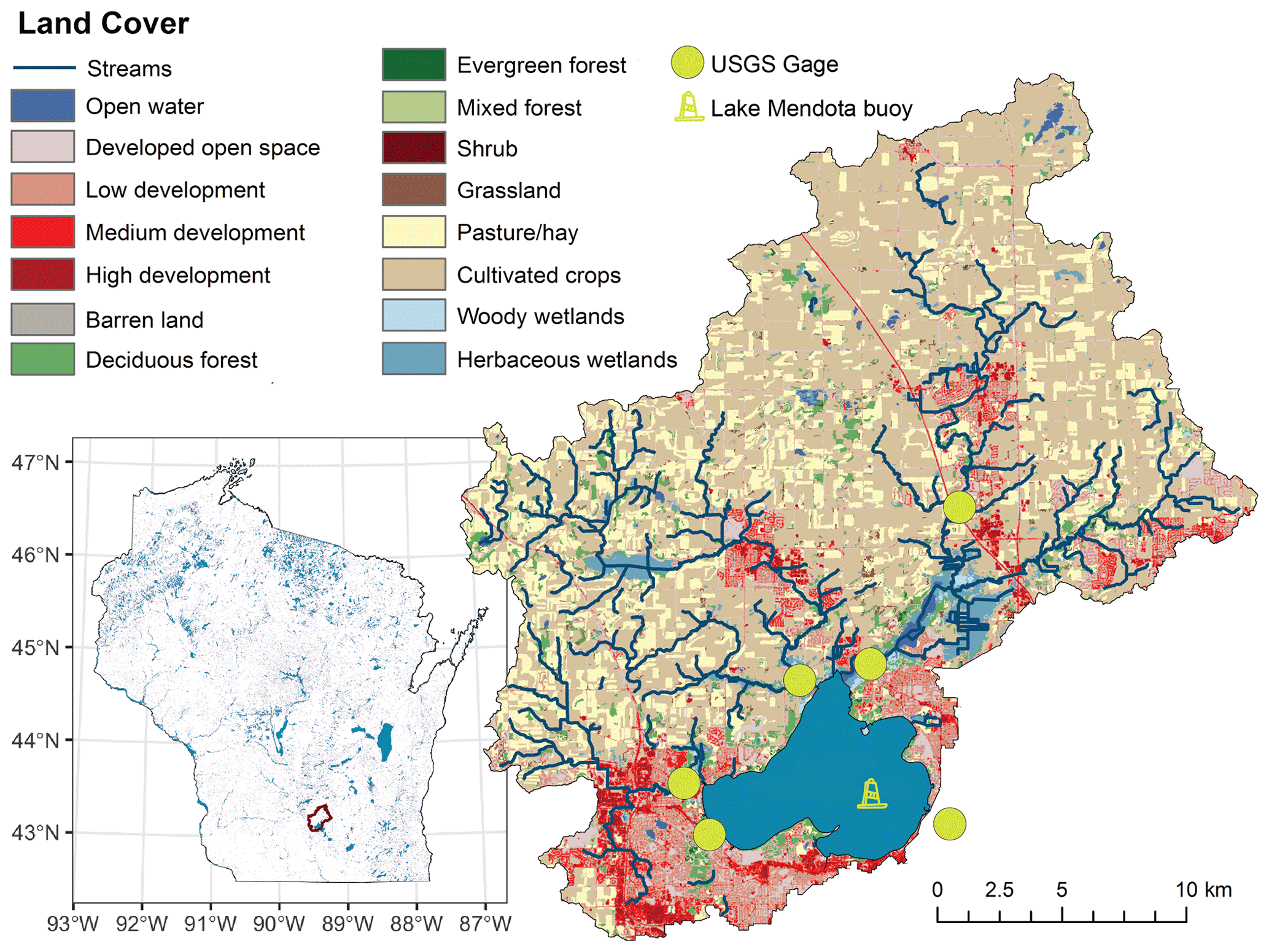
Figure 1 Location and overview map of Lake Mendota, Wisconsin, which is located in the Yahara River catchment in southern Wisconsin, USA. USGS gage stations for the PIHM-Lake model and the location of the Lake Mendota monitoring buoy are placed in the map. Land cover was sourced from the open-access US National Land Cover database.

2.2 Driver data acquisition

Meteorological forcing data were obtained from the second phase of the North American Land Data Assimilation System (NLDAS-2; Xia et al., 2012). The data from the grid cell were centered at 43^∘6^′3.4128^′′ N, 89^∘24^′37.1124^′′ W. The NLDAS-2 grid cells have $\mathrm{1}/\mathrm{8}$th-degree spacing and data are at an hourly resolution from 1 January 1979 to present (Mitchell, 2004). Meteorological parameters used in this study included wind speed, air temperature, specific humidity, surface pressure, surface downward short- and longwave radiation, and total precipitation, which were used primarily as boundary data for GLM-AED2. Relative humidity was calculated post hoc as a function of specific humidity, air temperature, and surface pressure.

To quantify the water budget in Lake Mendota, we simulated the water inflow from the catchment (through stream flow, overland flow, and groundwater flow) to the lake and water outflow from the lake to the catchments using a physically based distributed hydrologic model, PIHM-Lake (Penn State Integrated Hydrologic Model, see Supplement text “PIHM-Lake description”, Qu and Duffy, 2007). PIHM-Lake integrates hydrologic processes in a lake-catchment coupled system simulating the surface and subsurface hydrologic interactions within the catchment and between the catchment and the lake. Hydrologic interactions within the catchment are modeled in three dimensions, while the lake is represented in PIHM-Lake as a simplified one-dimensional bucket model assuming a uniform lake surface area and depth. PIHM-Lake tracks the change in water storage from the watershed's vegetation canopy, ground surface, unsaturated soil zone, saturated soil zone, and lake by using the semi-discrete finite volume method and a triangular irregular network (TIN). The PIHM-Lake simulation covers a 37 year period (from 1979 to 2015), and its parameters were calibrated and validated with in-situ measured stream inflow and lake outflow discharges from the US Geological Survey (USGS). The application of the PIHM-Lake model for quantifying the lake inflows helped close the water balance of Lake Mendota as groundwater inflow and surface overland flow were not measured and the model simulations provided these inflows.

Surface nutrient loadings from the Yahara River and Pheasant Branch inflows into Lake Mendota were estimated by regression models using discharge and nutrient concentration data from USGS gages (Appling et al., 2015; data are available at Ladwig et al. (2021) via the Environmental Data Initiative). Combined with the simulated discharge time series from PIHM-Lake, these regressions were used to compute daily loading data. We included the following nutrients in the inflow boundary conditions: soluble reactive phosphate, adsorbed soluble reactive phosphate, dissolved organic phosphorus, particulate organic phosphorus, dissolved organic nitrogen, ammonia, nitrate, refractory dissolved organic carbon, dissolved inorganic carbon, and reactive silica. For a complete description of the inflow loading regressions, see Weng et al. (2020). To provide information regarding adsorbed soluble reactive phosphate, we doubled measured total phosphorus (TP) concentrations and applied specific ratios to individual phosphorus forms (Farrell et al., 2020; Snortheim et al., 2017; Weng et al., 2020). This put our estimates of TP near the upper range of previous load estimates. Bennett et al. (1999) estimated the long-term average annual TP load to be about 34 t, whereas our average annual TP load (with adsorbed phosphate) was about 50.6 t and ranged between 5.3 to 146.1 t (1979–2015). Our average annual TP load (without adsorbed phosphate) was about 25.3 t and ranged between 2.7 to 73.1 t (1979–2015), which is similar to previous annual TP load estimates of 15 to 67 t (Kara et al., 2012) and 10 to 80 t (Lathrop and Carpenter, 2014). By doubling our TP by adding adsorbed phosphate, we accommodate a potential TP load underestimation due to the importance of extreme storm events on particulate loads (Carpenter et al., 2018). As direct measurements of inlet loadings of refractory organic matter, dissolved inorganic carbon (DIC), and silica were not available, we used constant average values for the inflow loadings similar to the long-term mean values of the water column.

Monitored NTL-LTER data from 1995 to 2015 were used for model calibration and validation. Data included water temperature and dissolved oxygen concentrations (Magnuson et al., 2019a, 2020b) with a vertical spatial resolution of 1 m from the surface to 24 m. Data were measured biweekly during summer, monthly during fall, and once per winter. The dissolved oxygen data set was complemented with historical measured dissolved oxygen data from 1992 to 1994 (Soranno, 1995). NTL-LTER data also included pH, dissolved inorganic carbon, dissolved organic carbon, nitrate, ammonia, soluble reactive phosphate, and silica sampled at the depths 0, 3, 8, 10, 12, 14, 16, 18, 20, and 22 m (Magnuson et al., 2020a). Surface-integrated samples of epilimnetic chlorophyll a and Secchi depth were used to evaluate GLM-AED2's predictions of phytoplankton biomass and light extinction (Magnuson et al., 2019b, 2020b).

2.3 Modeling framework

Our modeling framework to investigate drivers of hypolimnetic anoxia consisted of three components (Fig. 2):

1. Deductive model: a deductive model formulated by Livingstone and Imboden (1996) was run on the monitored field data to characterize the empirical relationships between observed dissolved oxygen data and oxygen depletion processes and to quantify the contributions of water column and sediments to hypolimnetic oxygen demand (Fig. 2). The deductive model furthered our ecosystem-scale understanding of the partitioning between volumetric and areal oxygen depletion sinks in Lake Mendota. Therefore, this approach was used independently of the other modeling approaches as a “check” on the sediment oxygen demand rates of Lake Mendota used in GLM-AED2.

   • 2a.

     GLM-AED2: to gain a more mechanistic understanding of how processes driving oxygen depletion lead to ecosystem-scale oxygen dynamics, we used the vertical one-dimensional hydrodynamic–water-quality model, GLM-AED2 (Hipsey et al., 2019). GLM-AED2 uses meteorological, hydrological, and nutrient load data as inputs and predicts lake physical, chemical, and biological dynamics, including those of dissolved oxygen. The advantage of using GLM-AED2 is that it quantifies and tracks processes relevant to oxygen cycling using well-accepted physical and biogeochemical interactions that otherwise are difficult to infer from observational data alone (see Sect. 2.3.2, Fig. 2). Although GLM-AED2 is a deterministic model, hypolimnetic anoxia is an emergent ecosystem property that derives from a complex suite of interactions within the model (Snortheim et al., 2017). Therefore, we used GLM-AED2 to simulate and track states and fluxes of modeled variables.

   • 2b.

     Regression model: to derive generalized relationships between the interannual variation in hypolimnetic anoxia and the driving data, as well as the output from GLM-AED2, we used statistical models on our combined dataset of monitored and modeled data. Because the number of potential candidate predictors is high, we used a machine learning approach to determine the most significant predictors of seasonal hypolimnetic anoxia at the interannual scale (Fig. 2). These predictors were then used in a multiple linear regression to rank their influence on hypolimnetic anoxia.

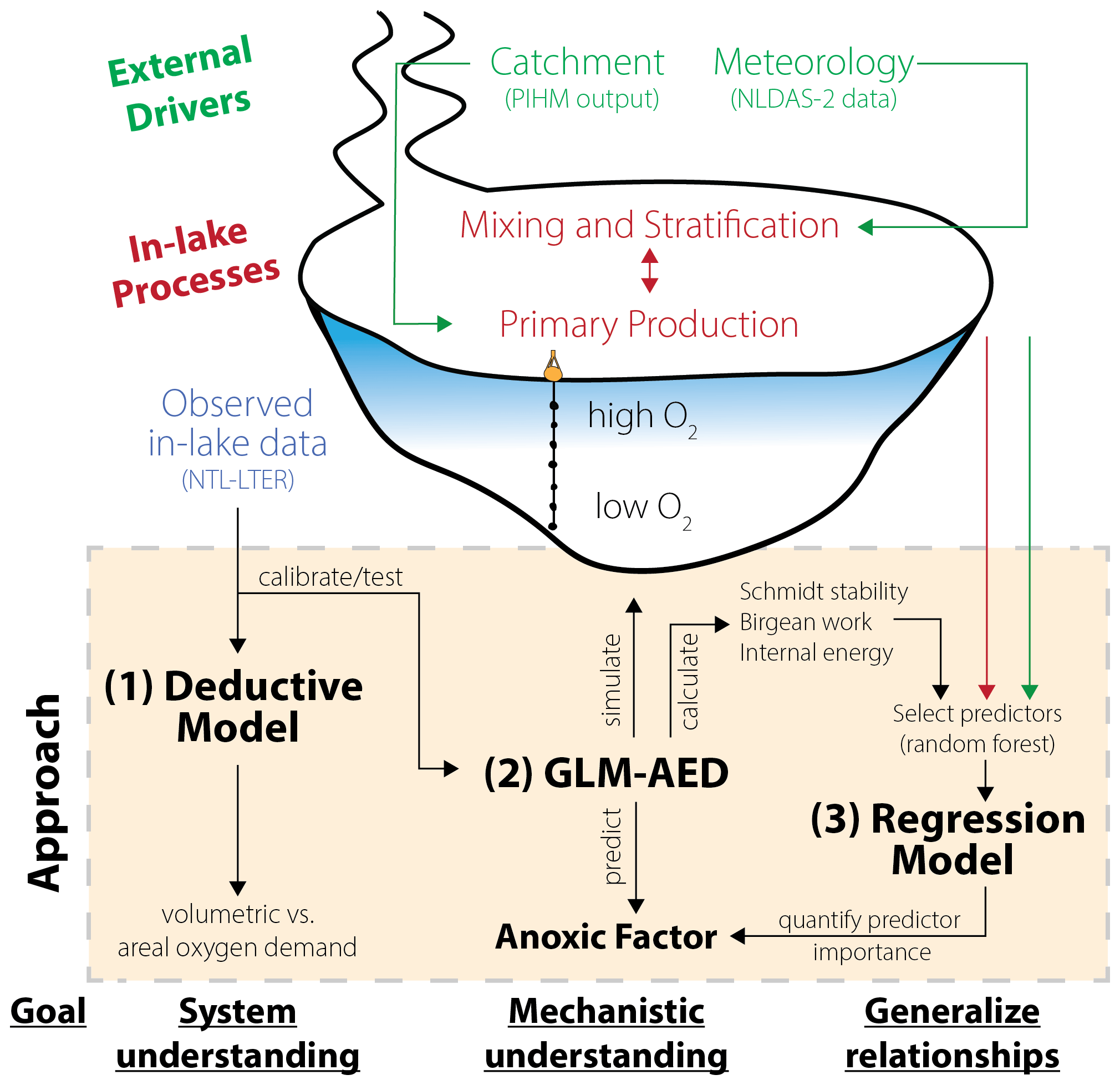
Figure 2 Schematic overview of the modeling workflow: (1) application of a deductive model to further our system understanding about oxygen sink terms; (2) replication of Lake Mendota using GLM-AED2 to investigate hydrodynamic and ecosystem mechanisms; and (3) application of regression models to quantify the importance of ecosystem predictors on the anoxic factor.

2.3.1 Deductive model

Using temporal and spatial linearly interpolated observed dissolved oxygen data, we applied the simple deductive oxygen depletion model according to Livingstone and Imboden (1996) in which the oxygen depletion rate J(z) at depth z is conceptualized as

$$\begin{array}{}\text{(1)}& J\left(z\right)=J_{\mathrm{V}}\left(z\right)+J_{\mathrm{A}}\left(z\right)\mathit{\alpha }\left(z\right),\end{array}$$

where the intercept J_V J_A is the volume sink (mass per volume per time) representing organic matter mineralization processes, e.g., microbial respiration in the water column, the gradient J_A is the area sink (mass per area per time) representing sediment oxygen demand, and α is a function for the ratio of sediment area to water volume over the depth z (Bossard and Gächter, 1981; Livingstone and Imboden, 1996):

$$\begin{array}{}\text{(2)}& \mathit{\alpha }\left(z\right)=-{\displaystyle \frac{\mathrm{1}}{A\left(z\right)}}{\displaystyle \frac{\mathrm{d}A\left(z\right)}{\mathrm{d}z}}.\end{array}$$

We used observed dissolved oxygen data from 1992 to 2015 (measured biweekly after ice offset) to calculate the specific oxygen depletion J(z) over depth for each year individually from the concentration, [DO]_spring, at the date of spring mixing offset, t_spring, to the date, t_2 mgL, when oxygen concentrations, [DO]_2 mgL, were below 2 mg L⁻¹ (criterion for hypoxia):

$$\begin{array}{}\text{(3)}& J\left(z\right)={\displaystyle \frac{[\mathrm{DO}{]}_{\mathrm{spring}}-[\mathrm{DO}{]}_{\mathrm{2}\mathrm{mgL}}}{t_{\mathrm{spring}}-t_{\mathrm{2}\mathrm{mgL}}}}.\end{array}$$

Only dissolved oxygen data below a depth of 15 m were used. The derivatives of area to depth were approximated by using forward and backward differencing. The terms J_V and J_A were assumed to be constant for every year (assuming the hypolimnion to be homothermic) and were determined by using weighted linear regression.

2.3.2 GLM-AED2

For simulating Lake Mendota, we used the coupled one-dimensional vertical hydrodynamic–ecological model GLM-AED2 (GLM: v.3.1.0a1, AED2: 1.3.4, developed by University of Western Australia; Hipsey et al., 2019). The hydrodynamic model GLM incorporates a flexible Lagrangian grid with each layer's thickness dynamically changing in response to the respective water density (Hipsey et al., 2019). Surface mixing processes are computed via an energy balance approach that compares the available (turbulent) kinetic energy to the internal potential energy of the water column (Hipsey et al., 2019).

The water quality module, AED2, was configured to simulate the dynamics of dissolved oxygen, silica, inorganic carbon, organic matter (refractory, particulate, and dissolved C, N, and P), and inorganic matter (refractory, particulate, and dissolved C, N, and P) as well as PO₄, NO₃, NH₄, and two functional phytoplankton groups (representing diatoms and cyanobacteria; Table S1 in the Supplement). The model was run on an hourly time step and output data were saved at a daily time step at noon. The thickness of each model layer (set to a maximum of 75 layers) could vary between 0.15 and 1.5 m with a minimum layer volume of 0.1 m³. The source code of the model's version, configuration files, and input and output data are stored and accessible at Ladwig et al. (2021) via the Environmental Data Initiative.

A global sensitivity analysis (Morris Method after Morris, 1991) was conducted to identify the most influential parameters for the predictions of water temperature, dissolved oxygen, dissolved inorganic carbon, silica, nitrate, and phosphate. Using the Morris method with 10 iterative runs, the distributions of the absolute elementary effects (the model change quantified by a fit function, here the root mean square error (RMSE) between observed and simulated data) of each parameter were calculated. According to Morris (1991) and Saltelli et al. (2004), the mean of the absolute elementary effects represents the overall sensitivity of the model outcome to each parameter, and the standard deviations are a metric of the interactions between different parameters. All parameters with a normalized mean elementary effect over 0.1 were declared sensitive and were used for the calibration.

According to our calculated absolute elementary effects, we included the following parameters in the calibration, listed according to their respective state parameter (Fig. S1 in the Supplement). For calibrating the six state variables, these parameters were (1) water temperature: bulk aerodynamic coefficient for sensible heat transfer (ch), longwave radiation factor (lw_factor), mean sediment temperature (sed_temp_mean), shortwave radiation factor (sw_factor); (2) dissolved oxygen: sediment flux (Fsed_oxy), mineralization rate of dissolved organic matter (Rdom), temperature multiplier for sediment flux (theta_sed_oxy); (3) dissolved inorganic carbon: sediment flux (Fsed_dic), half-saturation constant for oxygen dependence on sediment flux (Ksed_dic), temperature multiplier for sediment flux (theta_sed_dic); (4) silica: sediment flux (Fsed_rsi), half-saturation constant for oxygen dependence on sediment flux (Ksed_rsi), temperature multiplier for sediment flux (theta_sed_rsi); (5) nitrate: sediment flux (Fsed_nit), half-saturation constant for oxygen dependence on denitrification (Kdenit), half-saturation constant for oxygen dependence on sediment flux (Ksed_nit), maximum reaction rate of denitrification at 20 ^∘C (Rdenit); and (6) phosphate: sediment flux (Fsed_frp), half-saturation constant for oxygen dependence on sediment flux (Ksed_frp), temperature multiplier for sediment flux (theta_sed_frp).

We applied a combination of an automatic calibration technique and manual calibration for the calibration period from 2005 to 2015. First, the derivative-free, optimization algorithm (CMA-ES; Hansen, 2016) was used to minimize the RMSE between observed and simulated data (data were split into a calibration period, 2005–2015, and a validation period, 1995-2004). We used a time period prior to the calibration period for validation to stress test the model by applying it at a time period with potential different ecological characteristics. The model parameters were calibrated iteratively (and fixed for the next calibration step) in the following order: water temperature, dissolved oxygen, dissolved inorganic carbon, silica, nitrate, and, finally, phosphate. We did not calibrate for phytoplankton functional group biomass because it was out of scope for this analysis, but the model qualitatively recreated observed seasonal succession. Initial model parameter values were taken from default parameter values and ranges as well as literature values (Hipsey et al., 2017; Snortheim et al., 2017). Calibration of water temperature and dissolved oxygen concentrations were run for 300 iterations and the other variables for 200 iterations. The fit criteria were RMSE, Nash–Sutcliffe coefficient of efficiency (NSE), and Kling–Gupta efficiency (KGE; Gupta et al., 2009) for the calibration period, the validation period, and the total time period. The advantage of combining an automatic approach and a manual post-calibration for an overparameterized model such as GLM was that CMA-ES first limited the possible parameter space of each parameter, then in a second calibration step, parameters could be manually changed to improve overall dynamics and behavior without relying on a fixed objective function. The manual calibration was done to ensure that the model was not overoptimized with unrealistic parameter combinations of the biological parameters. This calibration approach was done in accordance with other aquatic ecosystem modeling studies (Fenocchi et al., 2019; Mi et al., 2020) that did not apply computational optimization to water quality models.

2.3.3 Post-processing of GLM-AED2 output

We quantified two heat budget metrics from simulated water temperature data: the Schmidt stability (Idso, 1973; Read et al., 2011; Schmidt, 1928) and the Birgean work (Birge, 1916; Idso, 1973). The Schmidt stability (St) is a stability index that expresses the amount of energy needed to mix the entire water column to uniform temperatures without affecting the amount of internal energy, whereas the Birgean work (B) is a stability index that quantifies the amount of external energy that is theoretically needed to build up the current stratification from a hypothetical completely mixed state. The sum of both terms, the total work G, gives an estimate of the energy needed to keep a lake isothermal during stratified conditions:

$$\begin{array}{}\text{(4)}& G=\mathrm{St}+B,\end{array}$$

$$\begin{array}{}\text{(5)}& \begin{array}{rl}G& ={\displaystyle \frac{g}{A_{\mathrm{s}}}}\underset{\mathrm{0}}{\overset{z_{\mathrm{m}}}{\int }}{A}_z\left(\mathrm{1}-{\mathit{\rho }}_z\right)\left(z_{\mathrm{v}}-z\right)\mathrm{d}z\\ & +{\displaystyle \frac{g}{A_{\mathrm{s}}}}\underset{\mathrm{0}}{\overset{z_{\mathrm{m}}}{\int }}{A}_z\left(\mathrm{1}-{\mathit{\rho }}_z\right)z\mathrm{d}z,\end{array}\end{array}$$

where g is gravity, A_s is the surface area (m²), z_m is the maximum depth (m), A_z is the respective area at depth z, ρ_z is the respective density at depth z (kg m⁻³), z_v is the depth of the center of volume ($z_{\mathrm{v}}=\frac{\mathrm{1}}{V}\underset{\mathrm{0}}{\overset{z_{\mathrm{m}}}{\int }}{A}_{z}z\mathrm{d}z$), and V is the volume (m³). The stagnancy of deep water can be quantified by calculating a heat budget ratio (HBR):

$$\begin{array}{}\text{(6)}& \mathrm{HBR}={\displaystyle \frac{G}{B}},\end{array}$$

which compares the amount of energy needed to maintain isothermal conditions to the amount of available external energy (Kjensmo, 1994). Here, an increased stagnancy of deep waters results in a reduced exchange of fluxes between the surface mixed and bottom layer. Therefore, HBR values > 1 indicate the isolation of the bottom water layers from surface fluxes in a lake.

Internal energy – as the stored thermal energy in the water column – was quantified using the R package rLakeAnalyzer (Winslow et al., 2019) as

$$\begin{array}{}\text{(7)}& E_{\mathrm{internal}}={\displaystyle \frac{\mathrm{1}}{A_{\mathrm{s}}}}\underset{\mathrm{0}}{\overset{z_{\mathrm{m}}}{\int }}{T}_z\cdot c_{\mathrm{w}}\cdot m_z\mathrm{d}z,\end{array}$$

where T_z is the water temperature at depth z (^∘C), c_w is the specific heat of water (J kg⁻¹ K⁻¹), and m_z is the mass of water at depth z (kg).

The thermocline depth was defined as a planar separation between the surface mixed and the bottom stagnant layer. The specific depth of this planar thermocline was quantified as the depth of the maximum density difference over the vertical axis where the minimum water temperature was above 4 ^∘C and the density difference between the surface and bottom layer was above 0.1 kg m⁻³, signaling stratified conditions.

The temporal and spatial extent of anoxia during the summer season was quantified using the AF:

$$\begin{array}{}\text{(8)}& \mathrm{AF}=\sum _{i=\mathrm{1}}^n{\displaystyle \frac{t_i{A}_i}{A_{\mathrm{s}}}},\end{array}$$

which sums the product of the anoxia duration t (d) with the corresponding area A (m²) to the total surface area A_swhen the in-water dissolved oxygen concentrations were below a threshold of 1 mg L⁻¹ (Nürnberg, 1995b). As the AF and hypoxic factor use the same equation with different thresholds relating essentially all anoxia information also to hypoxia, we focused on only quantifying the AF in this study. Observed AFs were calculated by temporally and spatially interpolating biweekly monitored field data using an ensemble of approaches (linear, constant, and spline interpolation between neighboring data points). We quantified the seasonal AF only for the summer season for the modeled and observed data. We then compared the modeled AF (quantified by using modeled daily dissolved oxygen data profiles) against a set of observed AFs (here, the biweekly data were temporally and spatially interpolated to get daily estimates over a finer vertical resolution) that were obtained by the application of three interpolation techniques.

2.3.4 Regression model

We evaluated 21 candidate predictors on their relative importance in predicting the simulated summer AF of the respective year n (see Table 1 for an overview and further explanation). All candidate predictors were either modeled output or boundary data for the model. This enabled the regression analysis to identify internal connections in the numerical model itself (similar analyses of modeled output and driver data were performed by Snortheim et al., 2017; Ward et al., 2020; Weng et al., 2020). For the calculation of certain candidate predictors, the water column was separated into an upper layer (from the surface to a depth of 10 m) and a lower layer (from 10 m to maximum depth). Although this is a rough approximation, this depth roughly represents the thermocline depth and further separates the water column into a zone without light limitation and one with light limitation.

Table 1 Overview of investigated predictors in a linear regression model on estimating the anoxic factor.

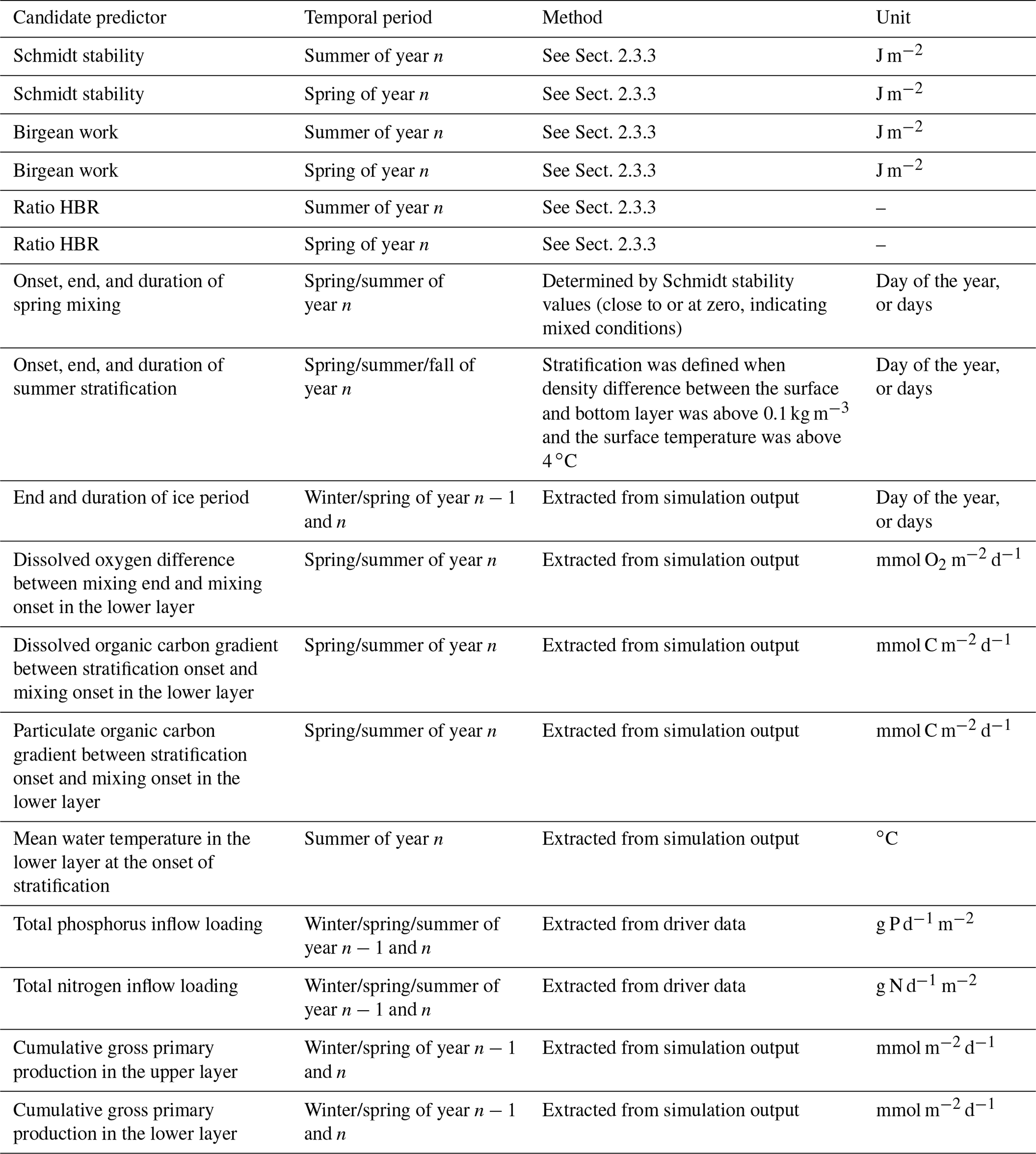
To represent external forcing processes, we included the seasonal total phosphorus inflow and seasonal total nitrogen inflow loadings for the pre-summer period (winter, spring, summer) of each respective year. Further, we included the Birgean work for spring and summer of each year, as the Birgean work represents the amount of external energy (mostly by wind shear stress) that is needed to build up the current thermal structure. In addition to the Birgean work, we also included the Schmidt stability; the HBR ratio; the onset, end, and duration of spring mixing; the onset, end, and duration of summer stratification; the mean hypolimnetic water temperature at the onset of stratification; and the end and duration of the ice period prior to summer to investigate the effects of physical control on hypolimnetic anoxia.

In-lake biogeochemical processes were represented by the dissolved oxygen concentration differences between spring mixing onset and offset in the hypolimnion (Livingstone and Imboden (1996) suggested that in eutrophic lakes, dissolved oxygen reductions during the mixing phase can have profound effects on the summer anoxia), organic carbon (both dissolved and particulate) concentration differences between spring mixing and stratification in the hypolimnion, and cumulative gross primary production in the epilimnion and hypolimnion. Organic matter gradients were investigated because dissolved organic carbon can be used as a proxy for allochthonous organic matter contributions to bacterial mineralization rates (Hanson et al., 2003). Gross primary production (GPP) was included as an example organic matter source that can fuel bacterial mineralization (Yuan and Jones, 2019). Here, GPP represents the sum of all the functional phytoplankton group's photosynthesis rates parameterized as the total carbon uptake:

$$\begin{array}{}\text{(9)}& \begin{array}{rl}{f}_{\mathrm{uptake}}^{{\mathrm{PHY}}_{\mathrm{C}}}=& R_{\mathrm{growth}}^{\mathrm{PHY}}\left(\mathrm{1}-k_{\mathrm{pr}}^{\mathrm{PHY}}\right){\mathit{\varphi }}_{\mathrm{temp}}^{\mathrm{PHY}}\left(T\right){\mathit{\varphi }}_{\mathrm{stress}}^{\mathrm{PHY}}\left(X\right)\\ & \min \left({\mathit{\varphi }}_{\mathrm{light}}^{\mathrm{PHY}}\left(I\right){\mathit{\varphi }}_{\mathrm{N}}^{\mathrm{PHY}}\left({\mathrm{NO}}_{\mathrm{3}}{\mathrm{NH}}_{\mathrm{4}}{\mathrm{PHY}}_{\mathrm{N}}\right)\right.\\ & \left.{\mathit{\varphi }}_{\mathrm{P}}^{\mathrm{PHY}}\left({\mathrm{PO}}_{\mathrm{4}}\mathrm{PHYP}\right){\mathit{\varphi }}_{\mathrm{Si}}^{\mathrm{PHY}}\left(\mathrm{Rsi}\right)\right)\left[\mathrm{PHY}\right];\end{array}\end{array}$$

where the carbon uptake $f_{\mathrm{uptake}}^{{\mathrm{PHY}}_{\mathrm{C}}}$ of an individual group PHY depends on the growth rate $R_{\mathrm{growth}}^{\mathrm{PHY}}$, the photorespiratory loss ($\mathrm{1}-k_{\mathrm{pr}}^{\mathrm{PHY}}$), temperature scaling ${\mathit{\varphi }}_{\mathrm{temp}}^{\mathrm{PHY}}\left(T\right)$, metabolic stress ${\mathit{\varphi }}_{\mathrm{stress}}^{\mathrm{PHY}}\left(X\right)$, and a minimum function taking into account limitations by light ${\mathit{\varphi }}_{\mathrm{light}}^{\mathrm{PHY}}\left(I\right)$, nitrogen ${\mathit{\varphi }}_N^{\mathrm{PHY}}\left({\mathrm{NO}}_{\mathrm{3}}{\mathrm{NH}}_{\mathrm{4}}{\mathrm{PHY}}_{\mathrm{N}}\right)$, phosphorus ${\mathit{\varphi }}_{\mathrm{P}}^{\mathrm{PHY}}\left({\mathrm{PO}}_{\mathrm{4}}{\mathrm{PHY}}_{\mathrm{P}}\right)$, and silica ${\mathit{\varphi }}_{\mathrm{Si}}^{\mathrm{PHY}}\left(\mathrm{Rsi}\right)$ (Hipsey et al., 2017; adapted from Hipsey and Hamilton, 2008). As the GPP is the main model output variable for phytoplankton dynamics, it scales directly with biomass and chlorophyll a concentrations.

To determine the relative importance of these candidate predictors that may influence the duration and extent of anoxia, we applied the Boruta R package (Kursa and Rudnicki, 2010) to identify the relevant predictors by using a wrapper built around a random forest classifier. The Boruta feature selection duplicates predictor values, which are then randomly shuffled to create so-called shadow attributes. If the variable predictor values (here the averaged accuracy loss normalized by the standard deviation and obtained from multiple random forest classifier runs) of the original values are significantly greater than the shadow predictor values, these variables are deemed relevant (Kursa and Rudnicki, 2010). Only model output and model driver data from the period 1980–2009 were used in the regression analysis. The first year, 1979, was dropped from the investigations due to a lack of prior winter information. The years 2010–2015 were dropped due to an apparent ecosystem shift (see Sect. 3.4). Meteorological quarterly divisions (DJF, MAM, JJA, SON) of the year were used to define seasons. After selecting important predictors driving the interannual variability in AF using the random forest method, we applied the remaining seven selected predictors in a multiple linear regression model to quantify their respective importance on predicting the AF. Stepwise model selection iteratively removed predictors to improve the regression model's AIC. This multiple linear regression model to predict AF included seven variables: the HBR ratio during spring, the HBR ratio during summer, the Birgean work in spring, epilimnetic GPP, the Schmidt stability in summer, the Birgean work in summer, and onset date of stratification. We reduced the complexity of the final multiple linear regression model to only three predictors of AF: onset date of stratification, the Schmidt stability in summer, and epilimnetic GPP in winter or spring. The Schmidt stability was included instead of the Birgean work as the resulting AIC of both models were similar, but the concept of the Schmidt stability is more commonly used in the limnological research community (Table S3 in the Supplement). The final multiple linear regression model was configured as (scaled predictors, adjusted R²=0.84, p<0.001; Table S4 in the Supplement)

$$\begin{array}{}\text{(10)}& \begin{array}{rl}\widehat{y}& =\mathrm{0.24}\mathrm{EpiGPP}+\mathrm{0.54}\mathrm{SummerSt}-\mathrm{0.46}\mathrm{OnsetStrat}\\ & -\mathrm{5.44}\times {\mathrm{10}}^{-\mathrm{17}}+\widehat{\mathit{ϵ}},\end{array}\end{array}$$

where $\widehat{\mathit{ϵ}}N(\mathrm{0},{\mathrm{38}}^{\mathrm{2}})$.

The relative importance of model fit was calculated as the R² contribution averaged over ordering among regressors (relaimpo package; Grömping 2006).

3 Results

3.1 Oxygen depletion rates

The derived annual oxygen depletion rates by the deductive model confirmed Lake Mendota's hypolimnetic anoxia as primarily driven by mineralization of organic matter. Observed oxygen depletion rates, J(z), against area–volume ratios, α(z), were positively correlated for all years except 1993, 1997, and 2007 (Fig. 3). For years with a positive relationship, the average intercept representing the volumetric sink J_V was 0.16 g m⁻³ d⁻¹ and the average gradient representing the areal sink J_A was 0.04 g m⁻² d⁻¹ (adjusted R²=0.13, p<0.001). Lake Mendota's hypolimnetic oxygen depletion was mainly driven by water column mineralization processes over sediment oxygen demand. The annual volumetric depletions rate followed a normal distribution with an increase in the volumetric sink in recent years. The areal depletion rate distribution was positively skewed. An inspection of the residuals from the model fits indicates that the linear regression model may not be appropriate for some years, especially for values of the sediment area to volume ratio α(z) near 0.5 m² m⁻³.

Figure 3 Regression plots of the morphometric function α(z) against oxygen depletion rates for the years 1992 to 2018, which were calculated from temporally linearly interpolated observed data. The respective equations represent weighted linear regressions.

Averaging this total oxygen depletion rate (volume and area sinks) over the hypolimnion gave a potential total oxygen depletion of ∼1 g m⁻² d⁻¹ (∼32 mmol [O₂] m⁻² d⁻¹). To conceptualize this depletion rate in our deterministic GLM-AED2 model, we used a maximum sediment oxygen demand (SOD) of 100 mmol [O₂] m⁻² d⁻¹. This rate represented the total sum of volumetric and areal oxygen sinks indirectly, as internal fluxes of organic carbon from the sediment back into the water column would drive additional oxygen depletion. This high value of SOD was scaled by the water temperature using an Arrhenius multiplier, effectively reducing it to a value between 1 to 1.5 g m⁻² d⁻¹ (32 to 47 mmol [O₂] m⁻² d⁻¹) of maximum oxygen depletion by the sediment sink in the hypolimnion during summer stratification. A recent modeling study investigating the formation of metalimnetic oxygen minima in a drinking water reservoir by Mi et al. (2020) confirmed that such high maximum SOD values are typical for many lakes.

3.2 GLM-AED2 calibration and validation

The thermal characteristics of Lake Mendota were replicated well, especially water temperatures in the surface layers (Table 2, Fig. 4, and Fig. S2 in the Supplement), with an RMSE of 1.30 ^∘C, an NSE of 0.97, and a KGE of 0.97, which is within the range of previous modeling studies (Bruce et al., 2018; Read et al., 2014). The simulated dissolved oxygen concentrations in the whole water column achieved an RMSE of 3.22 mg L⁻¹, an NSE of 0.56, and a KGE of 0.77. Here, the average fits were better in the surface layer (RMSE of 2.77 mg L⁻¹) compared to the bottom layer (RMSE of 3.31 mg L⁻¹), whereas the temporal dynamics (as expressed in NSE and KGE) were slightly better in the bottom layer (an NSE of 0.64 and a KGE of 0.81) compared to the surface layer (an NSE of −0.36 and a KGE of 0.47).

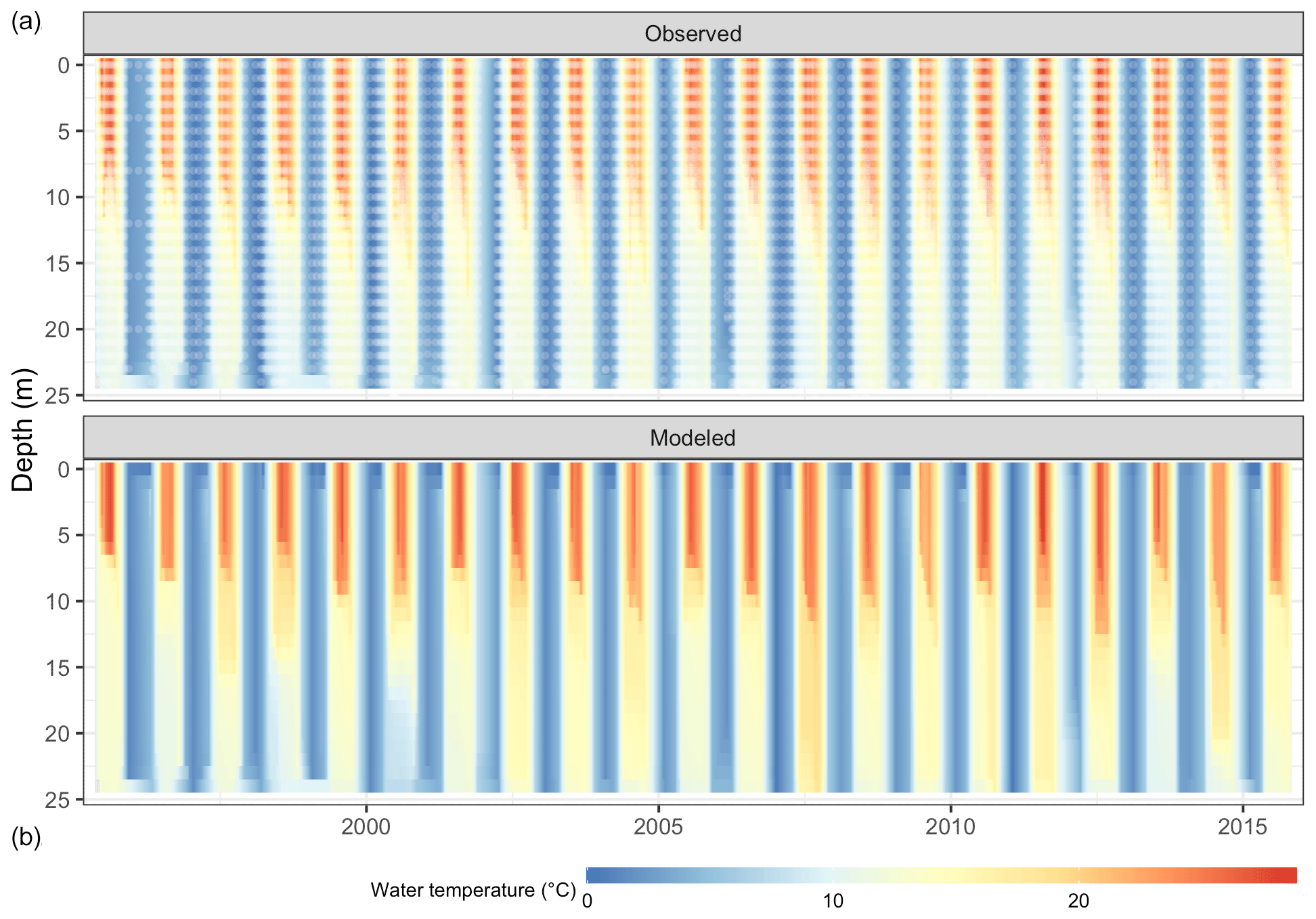
Figure 4 Comparison of Lake Mendota water temperature from observations (a, white dots mark sampling events) and GLM-AED2 simulations (b).

Table 2 Model performance for water temperature, dissolved oxygen, dissolved inorganic carbon, silica, nitrate, ammonium, and phosphate. During calibration and validation, only the total fits over all depths and time steps were calculated. Surface layers refers to a depth of 0 m below water table and bottom layer to a depth of 20 m below water table. Fits for surface and bottom layer during calibration and validation are not shown as the fit over the whole water column and over time were used.

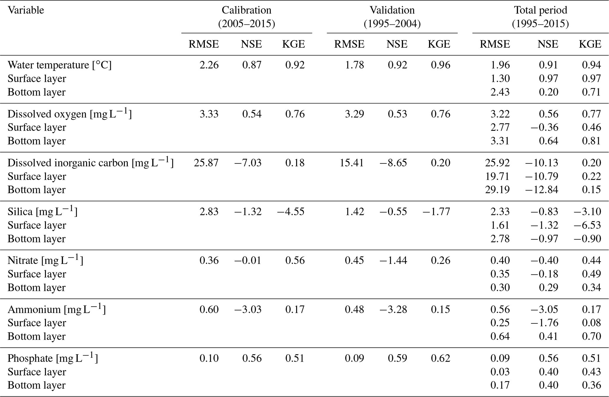
In contrast, the water quality model reproduced concentrations of the biogeochemical variables better at depth than at the surface, as evidenced by higher NSE values (Table 2, Figs. S3–S8 in the Supplement). The density distributions of residuals (observed minus simulated data) are in agreement (Fig. 5) for water temperature, dissolved oxygen concentrations, nitrate, phosphate, and ammonium (we did not use ammonium data during calibration but included it in the visual inspection to check general nitrogen dynamics replicated by the GLM-AED2 model), whereas the model overestimated dissolved inorganic carbon concentrations and chlorophyll a concentrations and underestimated silica concentrations. As described above, the inflow concentrations of DIC and silica were assumed to be constant over the simulation period, likely causing the discrepancies between model results and observed data.

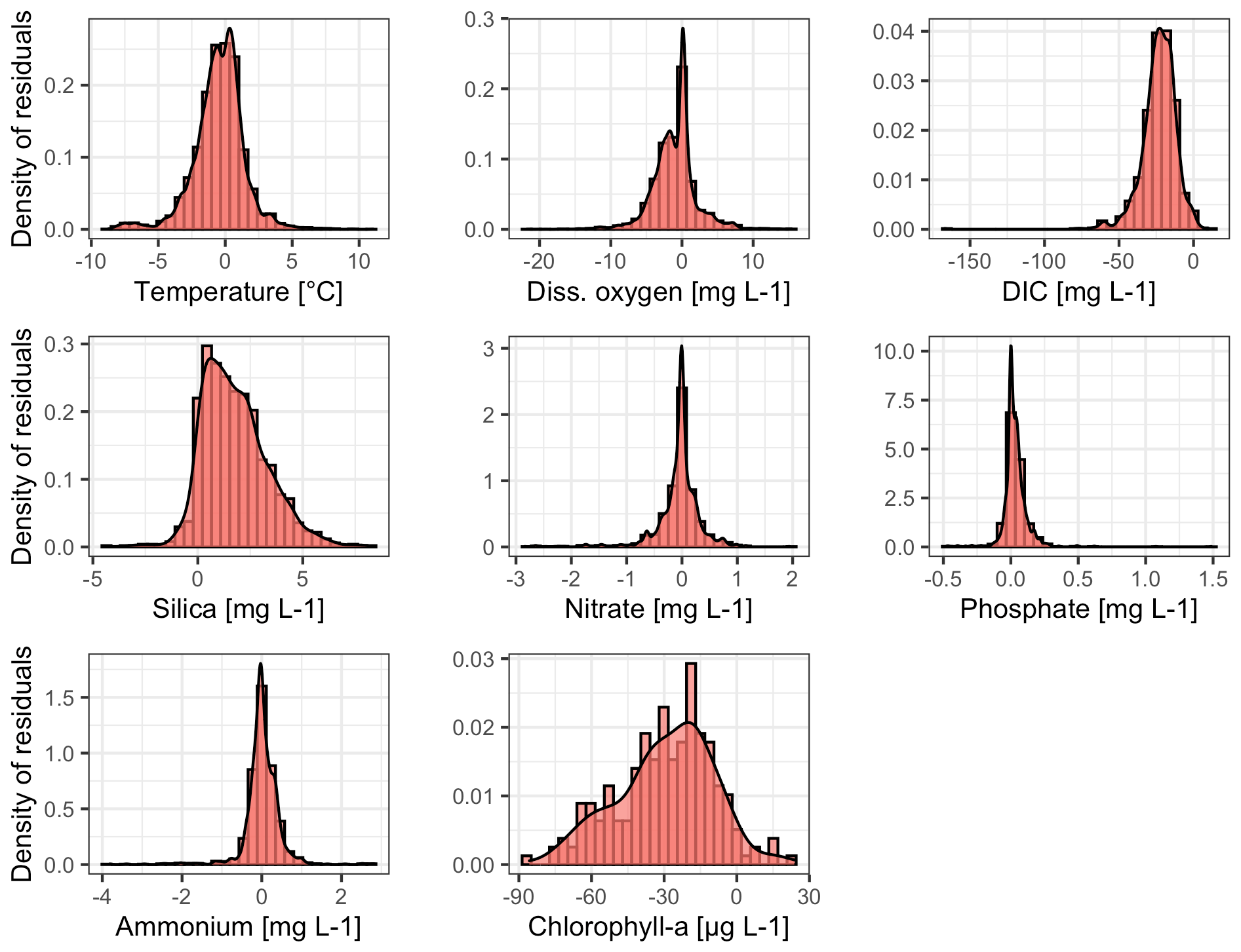
Figure 5 Density distributions of residuals (observed–modeled) for water temperature, dissolved oxygen, dissolved inorganic carbon (DIC), silica, nitrate, phosphate, ammonium, and phytoplankton. The density distributions include residuals over all data points (over each time step over each depth), calculated from observations minus model predictions.

3.3 Heat budget dynamics

Lake Mendota's annual stratification dynamics were characterized by a short spring mixing period followed by a very stable summer stratification period, which further promotes hypolimnetic oxygen depletion. A low Schmidt stability value in spring close to zero was representative of the overturn period (period I; Fig. 6). During this time, the Birgean work, as well as stored internal energy, increased rapidly and the water column remained well oxygenated. The spring overturn period (period I) was characterized by low HBR values (ratio of St+B to B) with an average of 0.85 (MMA in Fig. 7a). A low HBR denoted very unstable regimes due to an abundance of external energy compared to the required energy to keep the lake mixed. The start of the spring overturn period coincided with ice melt and open-water conditions, although in some years the thermal structure of the lake was well mixed prior to ice off and spring overturn. May was the earliest month when the average HBR was above 1 (Fig. 7b), which indicated that the water layers below the thermocline became isolated from the surface layers. Following period I, the Schmidt stability increased in conjunction with the spatial extent of anoxia in the lake water column (Fig. 6). The heat budgets, as well as the anoxic area, peaked during this second phase (period II) and declined, although the peak of the anoxic area lagged behind the heat budget peaks. As the Schmidt stability decreased to near zero in fall, mixing is initiated causing the water column to become oxygenated.

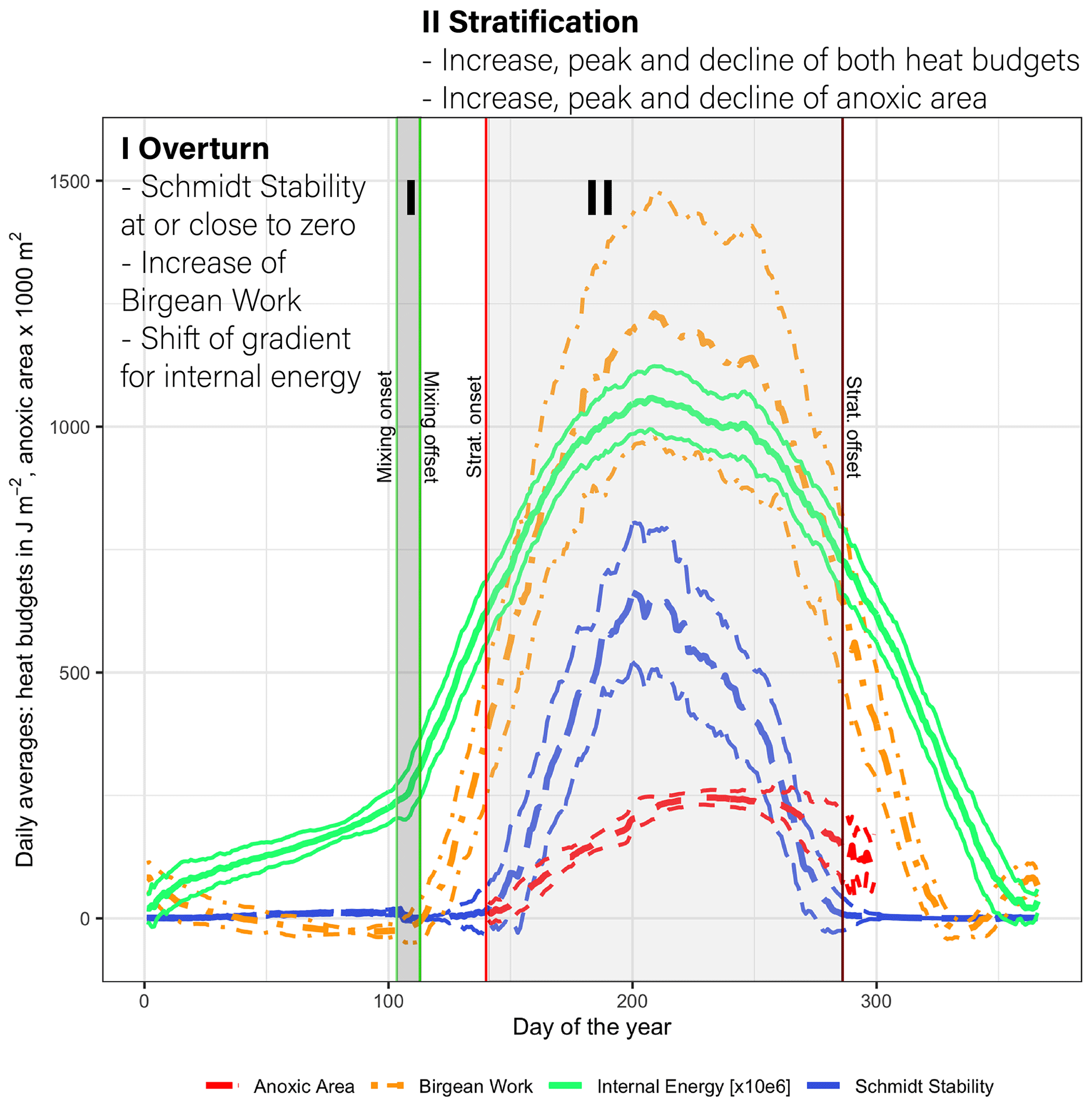
Figure 6 Daily average values of the Schmidt stability, the Birgean work, internal energy, and anoxic area (below 1 mg L⁻¹) plus or minus the respective standard deviations (dashed lines) (internal energy is given in 10⁶ J m⁻²). [Anoxic area units were adjusted for display.]

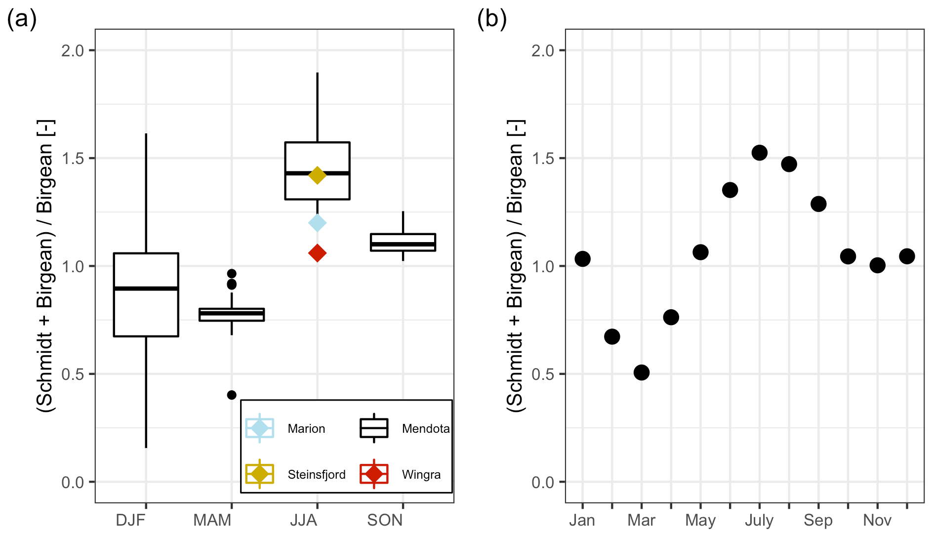
Figure 7 Dynamics of the average HBR = $(St+B)/B$ over time. (a) Boxplots of the HBR over the meteorological seasons, which represent seasonal quarters of the year beginning in December. The summer HBR values for Lake Marion, Lake Steinsfjord, and Lake Wingra were taken from Kjensmo (1994). (b) Scatterplot of the average HBR values for each month.

The stratification phase (period 2) had an average HBR value of 1.45, which indicated that an additional energy input of 45 % would be needed to keep Lake Mendota isothermal during stratified summer conditions (Fig. 7a). Lake Mendota's mean summer HBR value was similar to Lake Steinsfjord, Norway (max. depth 22 m; Kjensmo, 1994) and was larger than the HBR values of the unstable lake systems of Lake Marion, USA (max. depth 4.5 m), and Lake Wingra, USA (max. depth 6.1 m; Kjensmo, 1994). The oxygenation of the water column lagged behind the stratification period, and even when the Schmidt stability values at the end of the 2nd period were close to zero, a certain amount of the lake's area can remain anoxic.

Heat storage in Lake Mendota began after ice off and increased rapidly between the end of the mixing period and the onset of stratification (Fig. 8a). The amount of internal energy stored at the beginning of stratification correlated with the maximum available amount of internal energy that will be stored during the stratified period despite year-to-year fluctuations in internal energy. Over the course of each year, the amount of stored internal energy was positively correlated with the Schmidt stability (Fig. 8b). The Birgean work was also positively correlated with both the Schmidt stability and internal energy. The relationship between the Schmidt stability and the spatial anoxia extent exhibited a clockwise hysteresis (Fig. 8c). Beginning in June, the Schmidt stability increased as stratified conditions established in the water column. The Schmidt stability peaked on average in August at ∼720 J m⁻² (Fig. 6), followed by a peak in the Birgean work at ∼1250 J m⁻². Simultaneously, the depth of anoxia in the water column (anoxia height) followed the progression of the Schmidt stability, peaking in September. In Lake Mendota, the anoxia height was limited by the thermocline depth, as the low vertical turbulent diffusivity of the thermocline acted as a barrier for an encroachment of anoxic conditions into the surface mixed layer. Anoxia height decreased after September as the Schmidt stability decreased. Thermocline depth and anoxia height declined in parallel until the Schmidt stability reached zero. In Lake Mendota, as in most lakes, the surface layer was the region of significant heat storage (Fig. 8d). Once stratified, heat storage in deeper water layers was limited, whereas heat in the upper 5 m of the lake increased throughout the summer and accounted for up to 40 % of the total internal energy stored during summer.

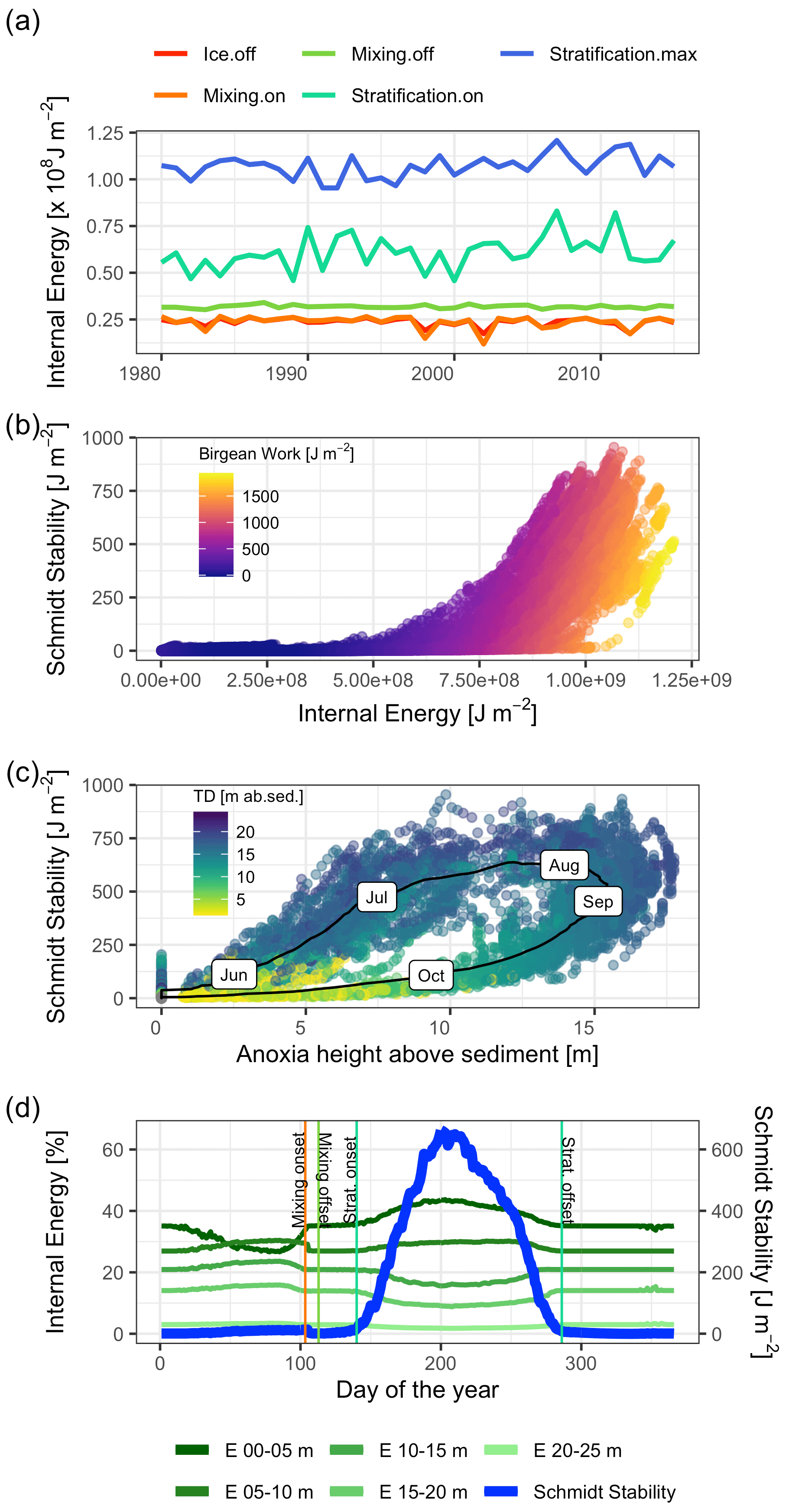
Figure 8 Stored heat dynamics and relationships to stratification strength, thermocline depth, and anoxia height (hypsographic height of anoxia area in the lake above sediment). (a) Time series of internal energy at the respective dates of ice off, mixing onset, mixing offset, stratification onset, and stratification offset. (b) Scatter plot of internal energy against the Schmidt stability. The color represents the magnitude of the Birgean work. (c) Scatter plot of anoxia height against the Schmidt stability. The black line represents the average dynamic over the course of a year with the respective months as labels. The color corresponds to the thermocline depth in meters above the sediment. (d) Time series of daily averaged internal energies stored over different depths and the Schmidt stability. The main heat storage happens in a shallow surface layer effectively after ice off and the simultaneous onset of a mixing period.

3.4 Oxygen dynamics

Dissolved oxygen dynamics, including the spatial extent of oxygen depletion in the water column and the timing of summer anoxia periods, were replicated by the GLM-AED model (Fig. 9a and b, Table 2), although the model overestimated spring and summer time surface oxygen concentrations due to a higher net ecosystem production. The depth-averaged fit criteria of dissolved oxygen concentrations were similar but slightly higher than reported in a recent study by Farrell et al. (2020) in which the RMSEs were 1.88 and 2.49 mg L⁻¹ in the epilimnion and hypolimnion, respectively, of a GLM-AED model calibrated for Lake Mendota. Our model captured annual anoxia events in the hypolimnion (Fig. 10a), and the range of the simulated AF was similar to the derived AF from observed data (Fig. 10b). The model failed to replicate extreme events (e.g., the very low AF in 2002) and did not capture a recent positive trend of AF since 2010. The simulated AF over the total time period averaged 56.7±5.2 d with an RMSE of 7 d, an NSE of −0.22, and a KGE of 0.26 (correlation coefficient r=0.28). The model's underestimation of the recent positive trend of AFs starting in 2010 was investigated by quantifying the fits during two periods: 1992–2009 (Fig. 10c) and 2010–2005 (Fig. 10d). In the pre-2010 period (1992–2009), the model achieved an RMSE of 6.79 d, an NSE of −0.25, a KGE of 0.44, and an r of 0.45 for AF predictions. In the post-2010 period (2010–2015), the model achieved an RMSE of 8.04 d, an NSE of −31.99, a KGE of 0.21, and an r of 0.62. A subsequent Wilcoxon signed-rank test highlighted that the observed average and modeled AFs from the pre-2010 period showed no significant differences between the two distributions, suggesting they belong to the same population (p value = 0.13; Fig. S9a in the Supplement), whereas the distributions of observed mean AFs and modeled ones after 2010 were significantly different (p value = 0.032; Fig. S9b in the Supplement), highlighting a potential decadal shift in oxygen depletion patterns. On the contrary, the modeled AF distributions of the pre- and post-2010 period were not significantly different (p value = 0.49; Fig. S9c in the Supplement), whereas the distributions of the observed AFs were significantly different (p value = 0.0049; Fig. S9d in the Supplement).

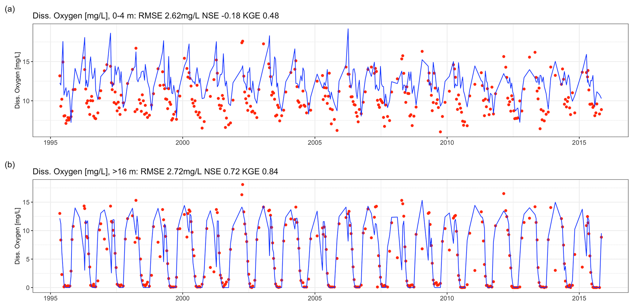
Figure 9 Time-series comparison between observed (red dots) and modeled dissolved oxygen concentrations (blue lines). The fit criteria were root mean square error (RMSE), Nash–Sutcliffe coefficient of efficiency (NSE), and Kling–Gupta coefficient of efficiency (KGE). (a) Averaged dissolved oxygen concentrations in the epilimnion (0–4 m). (b) Averaged dissolved oxygen concentrations in the hypolimnion (deeper than 16 m).

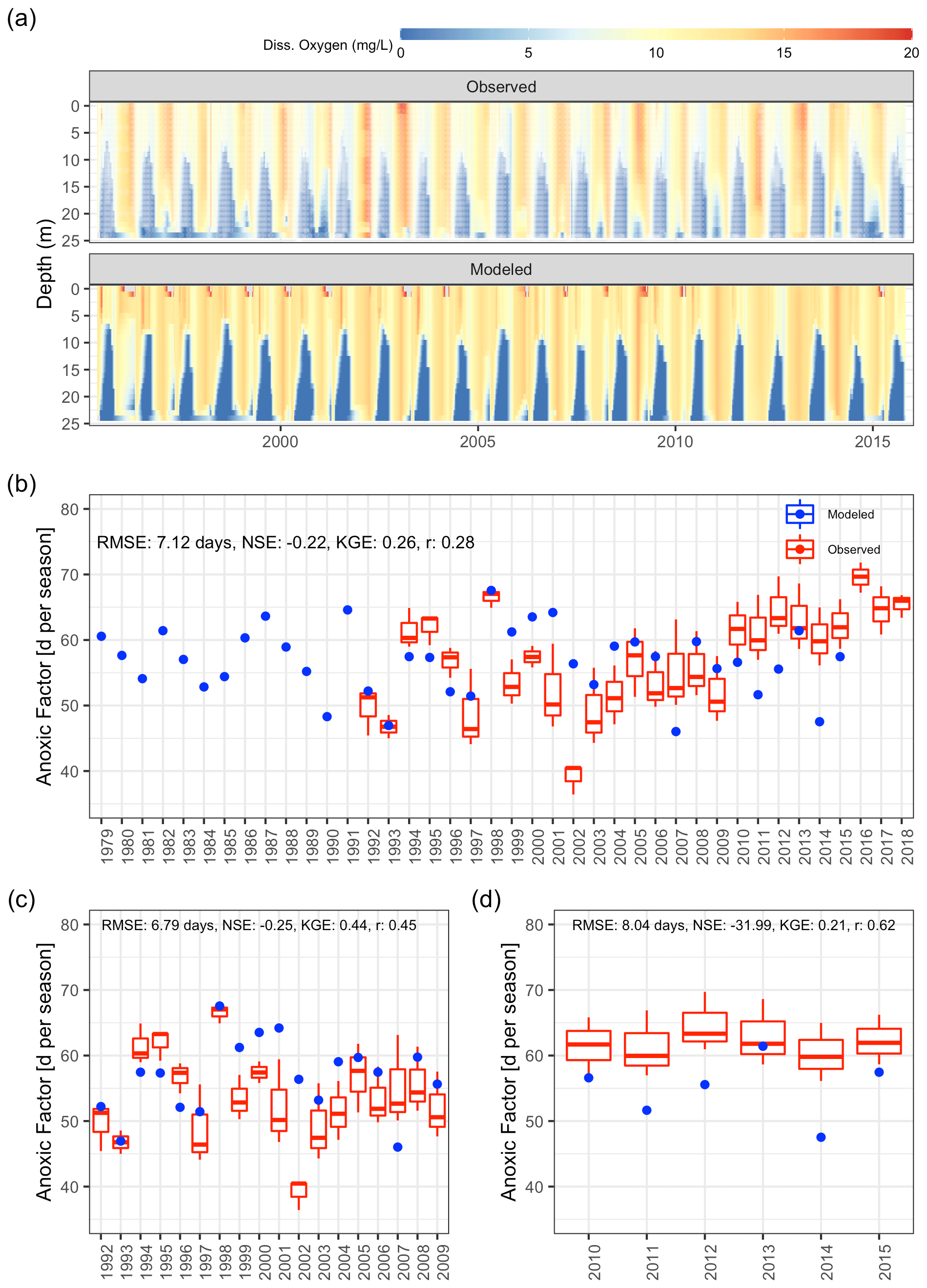
Figure 10 Comparison of observations to GLM-AED modeled dissolved oxygen concentrations and ecosystem response. (a) Contour plot of observed (upper figure, white dots mark sample events) and simulated dissolved oxygen concentrations. (b) Comparison of simulated anoxic factor (blue dots) against interpolated range of anoxic factor derived from observed data (box–whisker plots) over the period 1979 to 2018. (c) Comparison of simulated anoxic factor (red dots) against interpolated range of anoxic factor derived from observed data (box–whisker plots) over the period 1992 to 2009. (d) Comparison of simulated anoxic factor (red dots) against interpolated range of anoxic factor derived from observed data (box–whisker plots) over the period 2010 to 2015.

3.5 Regression model

We included in total three predictors in our final multiple linear regression, which were deemed important by the Boruta algorithm and stepwise linear model investigations using AIC for the period 1980–2009, namely the Schmidt stability during summer (rel. importance of 43 %), the onset date of stratification (rel. importance of 42 %), and winter to spring gross primary production in the epilimnion (rel. importance of 15 %; Table S4 in the Supplement).

The linear model showed a good agreement between simulated and predicted AF (Fig. 11a; Table S4 in the Supplement). The AF was positively correlated to the summer Schmidt stability (r=0.72; Fig. 11b) and the gross primary production in the epilimnion (r=0.48). It was negatively correlated to the onset of stratification ($r=-\mathrm{0.78}$; Fig. 11b).

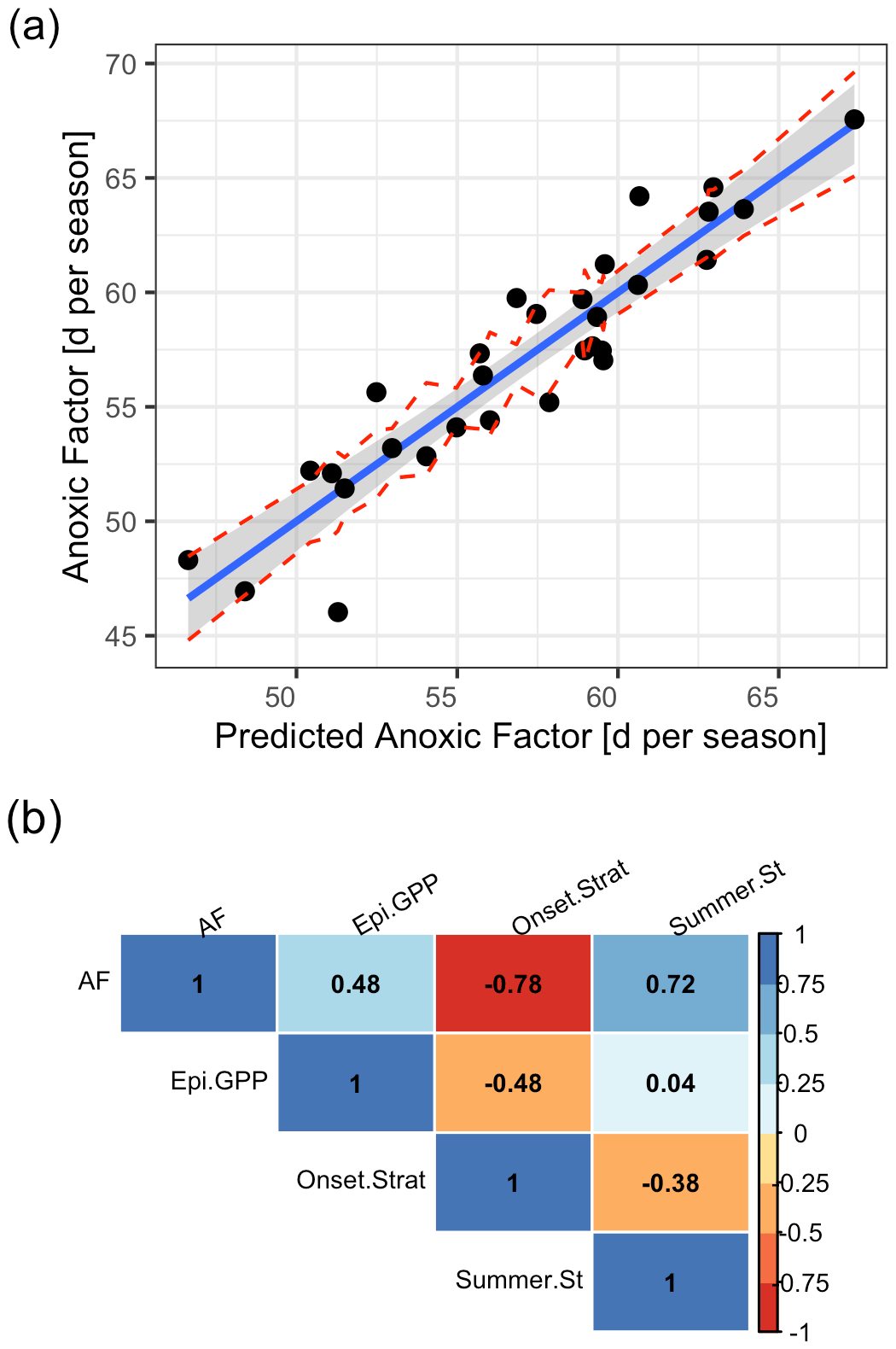
Figure 11 Predicted against simulated summer anoxic factor. (a) Linear model with a prediction that was done using a multiple linear regression model of the form $\widehat{y}=\mathrm{0.24}\mathrm{Epi}.\mathrm{GPP}+\mathrm{0.54}\mathrm{Summer}.\mathrm{St}-\mathrm{0.46}\mathrm{Onset}.\mathrm{Strat}-\mathrm{5.44}\times {\mathrm{10}}^{-\mathrm{17}}+\widehat{\mathit{ϵ}}$, where $\widehat{\mathit{ϵ}}N(\mathrm{0},{\mathrm{38}}^{\mathrm{2}})$. The red lines represent confidence intervals. (b) Correlogram of the input data using Pearson correlation coefficients. (AF = anoxic factor; Epi.GPP = gross primary production in the epilimnion prior to summer season; Summer.St = summer Schmidt stability; Onset.Strat = day of the year of summer stratification onset.)

4 Discussion

4.1 Controls of interannual variability on hypolimnetic anoxia

Interannual variability in the AF for Lake Mendota is influenced primarily by physical processes that regulate thermal and stratification dynamics, and less so by processes that influence organic matter. The Schmidt stability during summer (rel. importance of 43 %) and the timing of stratification (rel. importance of 42 %) both influence AF and are driven mainly by atmospheric drivers and heat convection throughout the water column. The most important predictor of AF directly related to biological processes is gross primary production in the epilimnion (rel. importance of 15 %; Table S4 in the Supplement) prior to summer. For eutrophic lakes, this suggests two critical points. First, climate has direct control over lake phenology. Climate drives the timing of stratification onset and stratification strength, and that controls the year-to-year variability in AF. Second, biology matters, but its interannual dynamics are not that influential, at least for this eutrophic lake with a residence time greater than one year. We also acknowledge that a step change in the AF occurred in 2010 and was unexplained by our model. Although the cause remains unknown, the timing was coincident with large increases in the invasive zooplankton Bythotrephes (Walsh et al., 2017).

4.2 Physical control over anoxic factor

Our work demonstrates that oxygen dynamics in Lake Mendota are strongly governed by the stratification strength and timing in the water column. Snortheim et al. (2017) came to a similar conclusion in an analysis of Lake Mendota during a shorter time period (2007–2010), arguing that changes in the atmospheric boundary conditions – air temperature, wind speed, and relative humidity – are driving changes in the hypolimnetic anoxia development of Lake Mendota. Here, we link these atmospheric drivers to changes in the water column's stratification (as quantified by the Schmidt stability and Birgean work). Over our 37 year simulation, anoxia onset occurred in the days following stratification onset. During stratification, the establishment of a strong density gradient between the upper and the lower layers in the water column reduces vertical turbulent diffusivities and limits the downward flux of dissolved oxygen. Without any additional oxygen source (e.g., atmospheric fluxes or primary production), dissolved oxygen concentrations below the thermocline are rapidly consumed by bacterial mineralization of organic matter in the water column and sediment.

In Lake Mendota, the temporal and spatial extent of anoxia is limited by the length of the summer stratification period (e.g., onset and offset of stratification, heat storage in water column prior to stratification; see Fig. 6) and the stratification strength and thermocline depth (e.g., the Schmidt stability, wind shear stress; see Fig. 8), respectively. The number of days between the onset of spring mixing, which begins immediately following ice off, and summer stratification determines the maximum amount of internal energy stored in summer. An early spring overturn and a slightly later stratification start would lead to increased anoxia height in the water column, though not necessarily a higher AF, as the duration of anoxia could be shorter. The mixing period is essentially a turning point in the year for the gradient of the internal heat accumulation, which increases rapidly following mixing. Still, as most energy is stored in a thin surface layer, short-duration extreme wind events or cold weather periods can deplete that additional stored heat before summer stratified conditions are reached. The storage of heat simultaneously increases the Birgean work, and later the Schmidt stability, increasing the resistance of the water column to mixing and limiting vertical fluxes from the epilimnion to the hypolimnion and vice versa. In summer, a higher amount of stored internal energy is also related to a higher Schmidt stability, further increasing the spatial extent of anoxia. Ultimately, the spatial extent of anoxia is limited by the thermocline depth, as in all simulated years the anoxia height reaches a maximum during late summer when the thermocline depth was already deepening.

4.3 Biological control over anoxic factor

Gross primary production (GPP) in the epilimnion prior to summer stratification is a secondary, but still important, predictor of anoxia. GPP fuels the sinking of particulate organic carbon (POC) into deeper layers before the establishment of a thermocline. In the hypolimnion, POC is readily decomposed into DOC, mineralized by bacteria in the numerical model, and reflects the dissolved oxygen volume sink. Unexpectedly, factors controlling year-to-year variation in GPP, such as external loadings of nutrients (specifically nitrogen and phosphorus), are not evident in the anoxia patterns in Lake Mendota. This is likely due to the historically high autochthony of the eutrophic lake (Hart, 2017), with phytoplankton blooms documented back to the early 1900s (Lathrop, 2007), thereby minimizing the need for external nutrient loads to stimulate phytoplankton production. While biological contributions to volumetric and sediment oxygen demands are well described for a broad range of lakes (Gelda and Auer, 1996; Matzinger et al., 2010; Müller et al., 2012; Rippey and McSorley, 2009; Yuan and Jones, 2019), for eutrophic lakes the control over available organic substrate for hypolimnetic oxygen demand may depend more on internal processing (autochthony) than external subsidies (allochthony).

Although the model replicated well the long-term DOC dynamics (Fig. S8 in the Supplement), it also overestimated surface layer dissolved oxygen concentrations compared to the observed data. This overestimation must have a concomitant increase in organic matter as a consequence of photosynthesis and, in this case, in POC. Considering that our proxy for the dynamics of phytoplankton biomass is reasonably well predicted (Fig. 5), this suggests our overestimate of primary production results in an increase in POC that is exported from the epilimnion to the hypolimnion. Unfortunately, we do not have observed POC to calibrate this part of the model, but we feel it is likely that our model has overestimated the contribution of primary production to hypolimnetic organic matter and subsequent oxygen depletion.

The regression models showed that variables related to load dynamics were not significant predictors of AF over nearly four decades. The total phosphorus and nitrogen loads, change in dissolved oxygen during spring overturn, temporal change in organic carbon pools, and ice duration were not found to be important based on the random-forest classifier. Phosphorus cycling in Lake Mendota is complex, so it may not be surprising that load dynamics in any one year are, to a certain extent, uncoupled from the hypolimnetic oxygen demand (Hanson et al., 2020). The relatively long water residence time of Lake Mendota (approx. 4 years; McDonald and Lathrop, 2017), along with the high internal phosphorus loading rate, means that external phosphorus loads represent only about $\mathrm{1}/\mathrm{3}$ of the available phosphorus in the epilimnion (Soranno et al., 1997). Furthermore, high primary production rates that exceed the total lake mineralization, along with external loads of organic carbon, lead to a high storage of organic matter in the sediments that can likely carry over from one year to the next (Hart, 2017). In a more nutrient-poor system, the nutrient and carbon availability would likely be more important predictors.

The model replicated the maximum anoxia event in 1998 but struggled to replicate the minimum in 2002. The discrepancies of 5–10 d between the simulated and observed range of the AF beginning in 2010 are related to an increased spatial and temporal extent of summer anoxia (Fig. S10 in the Supplement), which were not captured by the model. A similar increase in observed AFs starting in 2010 was also visualized in the study by Snortheim et al. (2017), but possible causes were not discussed. The increased spatial and temporal extent of summer anoxia were highlighted by the statistical analysis of the pre-2010 (1992–2009) and post-2010 (2010–2015) AFs. Prior to 2010, there were no significant differences between observed and modeled distributions (p=0.13), whereas after 2010 the observed distribution was significantly higher than the modeled distribution (p=0.032; Fig. S9 in the Supplement). Similarly, the pre-2010 observed AFs were significantly different than the post-2010 observed AFs (p=0.0049). For simplicity and due to limitations in Lake Mendota monitoring data post-2010, we focused the regression analysis of the AF in this study only on the pre-2010 period. The detection of this decadal shift in summer anoxia post-2010 highlights a hidden biological process that was not considered in the process-based model and may be due to an ecosystem shift in Lake Mendota that began in 2009 when the invasive spiny water flea (Bythotrephes longimanus) was detected in surprisingly high densities in the lake (Walsh et al., 2016b, 2018). The spiny water flea effectively became the dominant Daphnia grazer, causing historically low Daphnia biomass in 2010, 2014, and 2015 (Walsh et al., 2016a) and reducing water clarity. The spiny water flea may have increased organic matter supply to the hypolimnion by grazing down certain zooplankton and indirectly affecting phytoplankton. Mendota's Daphnia population historically consisted of Daphnia pulicaria and the smaller-bodied Daphnia galeata mendotae, which compete differently with the spiny water flea. D. mendotae biomass increased in spring after the spiny water flea invasion (Walsh et al., 2017), grazing on phytoplankton and probably accelerating organic matter mineralization before stratification onset. This could be one potential cause that contributed to the increase in hypolimnetic oxygen depletion after 2010. Our GLM-AED2 model could not replicate this food web change and subsequent shift in anoxia dynamics due to limitations of the numerical model, i.e., GLM-AED2 had constant ecological parameters over the entire modeling period and did not have zooplankton dynamics instantiated. We envision future monitoring and modeling studies of Lake Mendota that focus entirely on ecosystem shifts associated with the invasion of the spiny water flea in 2009 and the exponential growth of zebra mussels from 2015–2018 (Spear, 2020).

The simple deductive model established that the volumetric oxygen sink (i.e., water column oxygen demand) is consistently higher (on average about four times higher) than the sediment oxygen sink. The volumetric sink in lakes has been found to be strongly dependent on the trophic state of the lake, whereas the sediment sink is not (Rippey and McSorley, 2009). Eutrophic lakes tend to have high volumetric sinks that reach maxima of about 0.23 g m⁻³ d⁻¹ (Rippey and McSorley, 2009), similar to the average volumetric sink of 0.16 g m⁻³ d⁻¹ quantified by the deductive model for Lake Mendota. This finding is confirmed by the works of Conway (1972), who found that the high hypolimnetic oxygen demand of Lake Mendota was driven by algae decomposition originating from the surface layer. Although eutrophic lakes tend to have a high sediment oxygen demand, with specific values ranging from 0.3 g m⁻² d⁻¹ (Romero et al., 2004; Steinsberger et al., 2019) to extreme values of 80 g m⁻² d⁻¹ (Cross and Summerfelt, 1987), most studies measured or applied a value between 1 and 4 g m⁻² d⁻¹ (Mi et al., 2020; Veenstra and Nolen, 1991). The sediment oxygen demand calculated by our deductive model of 0.04 g m⁻² d⁻¹ was closer to the average value of approx. 0.08 g m⁻² d⁻¹ measured by Rippey and McSorley (2009) on 32 lakes. We note that the simple deductive model itself can only differentiate between two sources of depletion and neglects any physical transport drivers of oxygen, e.g., diffusion. Therefore, the results of the deductive model only add direct information to the actual depletion process of dissolved oxygen, but not of the dominant drivers.

4.4 Improving the modeling framework

The coupled GLM-AED2 model was able to generally replicate the thermal dynamics and biogeochemistry of Lake Mendota. In contrast to the calibration of Lake Mendota by Bruce et al. (2018) using an earlier version of GLM (v. 2.2.0), our model reproduced the water temperatures in the surface layer better than the bottom layer dynamics (RMSE for epilimnion and hypolimnion water temperatures, respectively, from Bruce et al., 2018: 1.94 and 1.42 ^∘C). This is probably due to the close proximity of the atmospheric forcing boundary condition to the surface layers, whereas the energy balance approach used by GLM potentially underestimates vertical mixing and hence overpredicts bottom layer water temperatures. In contrast, the model achieved better fits of the biogeochemical variables in the bottom layer. Better fits in the hypolimnion were likely achieved through directed calibration of sediment fluxes during the calibration–validation approach. The implementation and testing of alternative vertical mixing schemes for the Lake Mendota model (e.g., vertical mixing using a k−ε turbulence model) could potentially improve vertical transport and water temperature dynamics in deep layers. Further, using transient sediment boundary conditions with dynamic parameters over time could improve the model fit with the observed data and could replicate potential ecosystem shifts. As the spatial extent of hypolimnetic anoxia is fundamentally three-dimensional (Biddanda et al., 2018), fully resolving anoxia in space and time likely requires a three-dimensional model (Bocaniov and Scavia, 2016). Still, such a model has higher computational needs for long-term calibration–validation analysis, and current monitoring is inadequate to validate the results as most measurements are only made at the deepest point of the lake. Therefore, additional monitoring sites would need to be established. Improved spatial monitoring would be useful in validating our one-dimensional approach and setting up higher dimensional numerical models.

Our GLM-AED2 model overestimated spring phytoplankton biomass, which resulted in an overestimation of surface dissolved oxygen concentrations. This primary overproduction is a potential source of uncertainty for the anoxia timing below the thermocline, as the model's anoxia dynamics lag behind the observed ones. The time difference between the simulated and observed dissolved oxygen decline below the thermocline during stratification could be explained by an underestimation of sinking simulated organic material into the hypolimnion. Discrepancies between simulated and observed Anoxic Factors, therefore, could be rooted in our simplifications of the phytoplankton dynamics, the parameter calibration, and the related organic matter fluxes. These resulting discrepancies highlight the importance of improving the representation of phytoplankton and zooplankton dynamics in numerical models. Simulating a magnitude of individual species rather than functional phytoplankton groups has been shown to improve numerical water quality and ecosystem predictions (Hellweger, 2017), though it is unclear if it could improve spring bloom predictions in Lake Mendota. This also depends on a more extensive monitoring program that measures and specifies specific phytoplankton species over the vertical gradient on a regular basis. Further, better numerical representations of phytoplankton life cycles (Hense, 2010; Shimoda and Arhonditsis, 2016) and/or allometric scaling (Shimoda et al., 2016) could significantly improve numerical phytoplankton predictions. It is noteworthy that biweekly monitored data of Lake Mendota required interpolation of the observed data in order to calculate the observed AFs. This adds uncertainty to the observed AF, as monitoring likely missed important daily (or even sub-biweekly) fluctuations in dissolved oxygen.

It should be noted that as a statistical approach, the deductive regression model does not account for important mechanisms that may explain nonlinearities in the hypothetical linear relationships between the oxygen depletion rate and the sediment to volume rate. Thus, the deductive regression model may be biased for Lake Mendota. As the model still advanced our broader system understanding by quantifying the range of the sediment oxygen demand, it was still helpful to investigate observed dissolved oxygen concentration data.

4.5 Implications for landscape and climate change

The strong relationship between anoxia and water column stability suggests that a changing climate might increase the AF. Future climate in the region is expected to warm (Veloz et al., 2012), which may amplify and prolong water column stratification through increasing air temperatures (O'Reilly et al., 2015; Winslow et al., 2017). Shorter ice duration or even the total loss of ice (Sharma et al., 2019) could promote earlier heat storage in Lake Mendota, which could potentially increase the summer Schmidt stability, as demonstrated by Farrell et al. (2020). Earlier heat accumulation would cause a stability increase and an earlier onset of stratification, thereby extending the duration of anoxia. Further, a warmer epilimnion can cause the thermocline to become shallower during the course of summer, which would cause the anoxia height to be spatially limited by a layer that is closer to the surface; hence, more lake area would be anoxic. Increased oxygen depletion rates may also cause the anoxia height to be spatially limited by an earlier, and therefore lower, thermocline depth. Therefore, warming air temperatures will likely increase the AF of Lake Mendota through prolonged temporal and increased spatial extent of anoxia. It is worth noting that our initial regression quantified the correlation between AF and the water temperature in the hypolimnion at stratification onset as weakly negative. Higher water temperatures in a mixed water column prior to stratification onset are related to less stable stratified summer conditions. This feedback, potentially enhanced by shorter ice periods and warmer spring overturn periods, could shorten the extent of summer anoxia (similar findings were reported in Flaim et al., 2020).

Although our model evaluation supported the claim that external phosphorus loads are not important predictors of interannual variability in anoxia, future changes in the landscape (Motew et al., 2019), e.g., reduced agricultural application of phosphorus, less direct runoff pathways from the catchment to the lake, or more urbanization may change these relationships. Lakes with nutrient concentrations lower than Lake Mendota would almost certainly experience higher primary production with elevated nutrient loads, and higher primary production would likely fuel higher hypolimnetic respiration (Rippey and McSorley, 2009). Thus, the link between catchment processes and lake anoxia, which was not detectable in this study, would likely be important in lakes with meso- or oligotrophic states (Ward et al., 2020). For Lake Mendota, the only reasonable management approach to reducing anoxia is to lower external nutrient loads, especially given that anoxia duration in Lake Mendota is related to thermal stratification, which is predicted to increase with future warmer air temperatures.

5 Conclusions

We presented a novel modeling framework combining three complementary approaches (deductive model, numerical GLM-AED2 model, and regression model) to conceptually identify the important drivers of year-to-year variability in the spatial and temporal summer hypolimnetic anoxia extent of eutrophic Lake Mendota over a period spanning nearly four decades. Physical metrics – the summer Schmidt stability and onset date of stratification – were the most important predictors driving the summer AF. Although the gross primary production prior to summer stratification was still influential in affecting year-to-year variability of hypolimnetic anoxia, biological control over the AF was limited in our study period. As climate change is positively correlated to lake stratification characteristics (earlier, longer, and more intense summer stratification), we expect an increase in the AF of Lake Mendota in coming decades. The only local management option to mitigate future hypolimnetic anoxia in Lake Mendota is a reduction of external nutrient loads, which aims at shifting the lake towards oligotrophic conditions. Further, our modeling framework detected a decadal shift in the AF starting in 2010, which was not replicated by our process-based model and therefore probably not driven by physical or chemical drivers but related to an ecosystem shift caused by the invasive Bythotrephes longimanus. The modeling framework developed here can be extended by an advanced sediment diagenesis model and an uncertainty analysis, e.g., Bayesian analysis, to develop greater insight into effective strategies to mitigate environmental degradation. Consequently, as managers and decision makers work to prevent a decline in lake water quality as a result of climate change, decision support tools that support an understanding of lake dynamics over the long term are essential.