the Creative Commons Attribution 4.0 License.
the Creative Commons Attribution 4.0 License.
 | 23 Dec 2020
Key challenges facing the application of the conductivity mass balance method: a case study of the Mississippi River basin
Hang Lyu
Chenxi Xia
Jinghan Zhang
Bo Li
The conductivity mass balance (CMB) method has a long history of application to baseflow separation studies. The CMB method uses site-specific and widely available discharge and specific conductance data. However, certain aspects of the method remain unstandardized, including the determination of the applicability of this method for a specific area, minimum data requirements for baseflow separation and the most accurate parameter calculation method. This study collected and analyzed stream discharge and water conductivity data for over 200 stream sites at large spatial (2.77 to 2 915 834 km2 watersheds) and temporal (up to 56 years) scales in the Mississippi River basin. The suitability criteria and key factors influencing the applicability of the CMB method were identified based on an analysis of the spatial distribution of the inverse correlation coefficient between stream discharge and conductivity and the rationality of baseflow separation results. Sensitivity analysis, uncertainty assessment and T test were used to identify the parameter the method was most sensitive to, and the uncertainties of baseflow separation results obtained from different parameter determination methods and various sampling durations were compared. The results indicated that the inverse correlation coefficient between discharge and conductivity can be used to quantitatively determine the applicability of the CMB method, while the CMB method is more applicable in tributaries, headwater reaches, high altitudes and regions with little influence from anthropogenic activities. A minimum of 6-month discharge and conductivity data was found to provide reliable parameters for the CMB method with acceptable errors, and it is recommended that the parameters SCRO and SCBF be determined by the 1st percentile and dynamic 99th percentile methods, respectively. The results of this study can provide an important basis for the standardized treatment of key problems in the application of the CMB.
- Article
(5241 KB) - Full-text XML
-
Supplement
(112 KB) - BibTeX
- EndNote


Baseflow is the groundwater contribution to total streamflow (Hewlett and Hibbert, 1967), which plays a critical role in sustaining streamflow during dry periods (Rosenberry and Winter, 1997). Quantitative estimates of stream baseflow can be used to determine baseflow response to environmental conditions, thereby improving understanding of the water budget of a watershed and facilitating the estimation of groundwater discharge and recharge (Tan et al., 2009; Dhakal et al., 2012; Ran et al., 2012).
Given the importance of baseflow, many methods have been proposed for baseflow separation. Although these methods can be categorized according to various conditions (Stewart et al., 2007; Zhang et al., 2013; Miller et al., 2014; Lott and Stewart, 2016), they can generally be divided into two groups, namely non-tracer-based and tracer-based separation methods (Li et al., 2014). Non-tracer methods mainly include graphical and low-pass filter methods which only require stream discharge data (Nathan and McMahon, 1990; Eckhardt, 2008). Given the wide availability of stream discharge records, these approaches can readily be applied to a large number of sites (Miller et al., 2014). However, since these methods are typically applied without reference to any hydrological basin variables, the objective assessment of their accuracy remains a challenge (Nathan and McMahon, 1990; Arnold and Allen, 1999; Arnold et al., 2000; Furey and Gupta, 2001; Huyck et al., 2005; Eckhardt, 2008). In contrast, tracer-based baseflow separation methods adhere to the principle of mass balance (MB). Tracers such as stable isotopes, major ions and specific conductance (SC) have been used to quantify surface runoff and groundwater discharge to streamflow (Miller et al., 2014). The advantage of these methods relates to their use of site-specific variables, such as concentrations of chemical constituents, which are a function of actual physical processes and flow paths in the basin responsible for generation of different flow components. Therefore, chemical mass balance estimates of baseflow are often considered to be more reliable than those from graphical hydrograph separation estimates (Stewart et al., 2007). The principal disadvantage of mass-balance methods relates to their requirements of both observed discharge and chemical concentration data, which are not widely available, especially over a long period. This makes the application of the MB method in large basins impractical over a long period. For example, while stable isotopes are generally considered to be the most accurate chemical tracers for hydrograph separation (Kendall and McDonnell, 2012), the analytical costs associated with these constituents often limit their use in large studies (Miller et al., 2014).
In an analysis of hydrograph separation conducted using different geochemical tracers, Caissie et al. (1996) demonstrated that SC was the most effective single variable for quantifying the runoff and groundwater components of total streamflow since SC is a natural environmental tracer that can be inexpensively measured concurrently with streamflow (Kunkle, 1965; Matsubayashi et al., 1993; Arnold et al., 1995; Caissie et al., 1996; Cey et al., 1998; Heppell and Chapman, 2006; Stewart et al., 2007; Pellerin et al., 2008).
The conductivity mass balance (CMB) method converts specific conductance to a baseflow value using a two-component mass balance calculation (Pinder and Jones, 1969; Nakamura, 1971; Stewart et al., 2007):
In Eq. (1), Q is the measured streamflow discharge (L3 T−1), SC is the measured specific conductance (lS cm−1) of streamflow, SCRO is the specific conductance of the runoff end-member, and SCBF is the specific conductance of the baseflow end-member.
Certain questions need to be addressed before the CMB method can be considered for separating baseflow in a watershed. These include whether the CMB method is applicable to a watershed, how to more accurately determine the key parameters SCRO and SCBF when a long series of monitoring data are available, and the length of the monitoring period required to ensure the accuracy of the results when adopting a CMB method for a new conductivity monitoring network. These questions have been partially answered by past studies. Miller et al. (2014) concluded that the CMB method was successful in quantifying baseflow in a variety of stream ecosystems, including snowmelt-dominated watersheds (Covino and McGlynn, 2007), urban watersheds (Pellerin et al., 2008) and a range of other settings (Stewart et al., 2007; Sanford et al., 2011; Lott and Stewart, 2016). However, most chemical hydrograph separation studies have been conducted in small watersheds and for short durations (Miller et al., 2014). In addition, the CMB method is often not appropriate for application to systems in which there is no a consistent inverse correlation between discharge and SC, particularly for sites heavily influenced by anthropogenic activities. However, there appears to be no further systematic summary of characteristics of watershed systems that indicates the suitability of the CMB method. Questions therefore remain of how to determine whether the CMB method is appropriate for application to a particular watershed and which factors have the greatest impact on the outcome of the application of the CMB method. Further uncertainties in the CMB method relate to appropriate methods for determining the parameters of the method. Stewart et al. (2007) determined through a field test that the maximum and minimum conductivity can be used to replace SCBF and SCRO, respectively. Miller et al. (2014) found that the maximum conductivity of streamflow may exceed the real SCBF; therefore, they suggested the use of the 99th percentile of conductivity of each year as SCBF to avoid the impact of high SCBF estimates on the separation results and assumed that baseflow conductivity varies linearly between years. However, questions remain in relation to which parameter determination method is more reasonable and accurate for calculation of baseflow. In a study of the shortest monitoring period of the CMB method, Li et al. (2014) evaluated data requirements and potential bias in the estimated baseflow index (BFI) using conductivity data for different seasons and/or resampled data segments at various sampling durations, and they found that a minimum of 6 months of discharge and conductivity data are required to obtain reliable parameters with acceptable errors. However, their study conceded that further studies of watersheds at large temporal and spatial scales are needed to verify the conclusions.
The present study conducted a comprehensive qualitative and quantitative analysis of data from more than 200 hydrological sites widely distributed in the Mississippi River basin, United States of America. Based on the results of statistical analysis, the present study had the following objectives: (1) determine the criteria and main factors influencing the applicability of the CMB method; (2) identify the best method for determining the parameters of the CMB method; (3) determine data requirements for the CMB method. The conclusions of the present study can help to determine whether the CMB method is applicable to a particular river reach and can provide a reference standard for use of the method.
2.1 Data sources and site description
The Mississippi River basin is located on the western side of the continental divide. The basin encompasses five states and has a drainage area of 320 000 km2. A total of 201 sites were selected in watersheds of the Missouri, Illinois, Minnesota, Iowa, Ohio, Arkansas, Red, White and Des Moines rivers to represent the variability of sub-basin areas and physiographic and climatic regions, with the areas of sub-basins ranging from 2.77 to 2 915 834 km2 (Fig. 1). Each selected site had at least 2 years of continuous discharge data paired with specific conductance data. All discharge and specific conductance data used in the present study were mean daily values retrieved from the United States Geological Survey's (USGS) National Water Information System (NWIS) website (http://waterdata.usgs.gov/nwis, last access: 10 March 2019).

Figure 1Map showing the Mississippi River basin and the locations of the 201 stream gauging sites included in the present study.
2.2 Determination of the applicability of the CMB method and the identification of the major factors influencing the applicability of the CMB method
The CMB method assumes that the two main recharge sources in any particular river section, streamflow runoff and baseflow have relatively stable conductivity values (Stewart et al., 2007; Lott and Stewart, 2012). Under natural conditions, streamflow conductivity reaches a maximum value under the dry season minimum discharge, indicating the dominant contribution of baseflow to streamflow (Miller et al., 2014). In contrast, streamflow conductivity will decrease during the high-flow period when the contribution of direct runoff through rainfall or snowmelt to discharge increases. This relationship between stream conductivity and the discharge persists through intermediate-state streamflows, with an inverse power function between streamflow discharge and conductivity identified (Miller et al., 2014). Conditions under which the above general relationship does not apply indicate the influence of other external factors on the river which the CMB method would be unable to represent. Therefore, during the process of baseflow separation, the applicability of the CMB method to a particular river section can be determined by identifying the relationship between stream discharge and conductivity.
In the present study, to identify the applicability of the CMB method to the 201 different site locations in the Mississippi River basin, the relationships between conductivity and streamflow discharge at the sites were quantitatively evaluated by correlation analysis. Stream sites were grouped into four categories according to the strength of the relationship, as indicated by the inverse correlation coefficient (r): (1) high degree of inverse correlation (); (2) medium degree of inverse correlation (); (3) low degree of inverse correlation (); (2) no inverse correlation (). The present study analyzed the spatial distribution of stream site correlation coefficients in the basin combined with statistical data on topography, stream discharge and anthropogenic activities. The influences of these factors on the inverse correlation were studied, following which the key factors affecting the applicability of the CMB method to sub-basins of different spatial scales were identified. Thus, a set of judgement criteria for the applicability of the CMB method for baseflow separation to a certain area was established.
2.3 Determination of the SCBF and SCRO
As according to the CMB equation (Eq. 1), the key parameters that are needed to calculate the baseflow index of total flow are the conductivities of baseflow (SCBF) and surface runoff (SCRO). It is generally believed that runoff dominates streamflow during the extreme high-flow and minimum stream conductivity periods of each year, during which stream conductivity is assigned as SCRO. In contrast, stream conductivity during extreme low-flow and maximum stream conductivity periods of each year is assigned as SCBF, during which baseflow dominates streamflow (Stewart et al., 2007; Lott and Stewart, 2012).
Several approaches are currently used to determine SCBF: (1) directly assigning the maximum stream conductivity of the stream monitoring record as SCBF (Stewart et al., 2007); (2) assigning the 99th percentile (ordered by increasing conductivity) of the stream conductivity monitoring record to avoid the impacts of extremely high SCBF estimates that may arise when river conductivity has been affected by factors such as evaporation, irrigation, mining activity and the use of salts as road de-icing agents on the separation results; (3) identifying yearly dynamic maximum or 99th percentile conductivity measurements within a monitoring record as SCBF (Miller et al., 2014).
Since Stewart et al. (2007) have pointed out that longer conductivity records are more likely to contain low conductivity values associated with high discharge, the present study used the minimum or 1st percentile (ordered by decreasing conductivity) method to estimate SCRO.
The sensitivities of BFI to SCBF and SCRO expressed as an index, i.e., S(BFI∕SCBF) and S(BFI∕SCRO), respectively, and the uncertainties of SCBF, SCRO and BFI, which can be expressed as , and WBFI, respectively, were calculated using the monitoring data of 26 stream sites with long-term records of stream discharge and conductivity for at least 5 years. The present study then proposed an optimal method of determining SCBF and SCRO according to an analysis of different methods for calculating baseflow hydrographs.
2.4 Data requirements for SCBF and SCRO
Monitoring data of 26 stream sites with long-term records of stream discharge and water conductivity were analyzed to study the influence of different monitoring durations on the accuracy of parameter determination and baseflow separation results. Among the 26 sites, 5 had monitoring periods longer than 14 years, whereas the remainder had monitoring periods longer than 5 years. Continuous sampling periods within the five longer stream monitoring records included 3, 6, 9, 12, 15, 18, 21 and 24 months, whereas those in the remaining stream monitoring records included 3, 6, 9 and 12 months. To reduce the sampling error caused by the small number of samples, overlapping of monitoring data was allowed when sampling. In addition, each segment for a specific sampling duration was randomly chosen due to the variability in water quality measurements (Li et al., 2014). SCBF, SCRO and BFI were calculated for each segment, following which it was determined whether the BFI of all segments for the specific sampling durations followed normal distributions. On the premise of following a normal distribution, the BFI values obtained using 3, 6, 9, 12, 15, 18 and 21 months of conductivity measurements were compared with the BFI values obtained with 24 months of data for the five sites with longer records. For the remaining sites, the BFI values obtained with 3, 6 and 9 months of conductivity measurements were compared with the BFI values obtained with 12 months of data. A Student's T test at a statistical significance level of 0.05 was used to examine the differences between BFI determined from data of each sampling duration and those from the 24 or 12 months of data. No significant difference in BFI values estimated with a shorter duration of conductivity records with those obtained with 24 or 12 months of data (P>0.05) indicated that the shorter time duration for conductivity measurement was acceptable.
2.5 Quantitative estimates of the sensitivity and uncertainty in baseflow
As mentioned above, the sensitivities of BFI measurement to SCBF and SCRO were calculated and the uncertainties of CMB results obtained using different parameter determination methods and monitoring durations were evaluated to identify the most accurate parameter calculation method and the shortest appropriate monitoring period.
The dimensionless sensitivity index of BFI (output) with SCBF (uncertain input) and SCRO, S(BFI|SCBF) and S(BFI|SCRO), reflecting the proportional relationship between the relative error in BFI and the relative error in parameters, were calculated using the following equations (Yang et al., 2019):
In Eqs. (2) and (3), y is streamflow (L3 T−1) and k is the time step.
There is uncertainty associated with the estimation of true means from finite samples, which is regarded as a type of error in statistical inference (Lo, 2005). This uncertainty in the CMB method was estimated based on the uncertainties in SCBF, SCRO, and SCk. Under the approach used in the present study, the errors in the input variables are propagated to output variables following the uncertainty transfer equation derived from (Genereux and Hooper, 1998)
In Eq. (4), fbf is the ratio of baseflow to streamflow in a single calculation process, is the uncertainty in fbf at the 95 % confidence interval, is the standard deviation of SCBF multiplied by the t value (α=0.05; two-tail) from the Student's distribution, is the standard deviation of the lowest 1 % of measured SC concentrations multiplied by the t value (α=0.05; two-tail), and is the analytical error in the SC measurement multiplied by the t value (α=0.05; two-tail). The average uncertainty in multiple calculation processes is then used to estimate the uncertainty in the baseflow index (BFI, long-term ratio of baseflow to total streamflow), which can be expressed as WBFI-Genereux (Genereux and Hooper, 1998; Miller et al., 2014).
On the other hand, Yang et al. (2019) found that random measurement errors in yk or SCk for time series exceeding 365 d will cancel each other out, allowing the influence on BFI to be ignored. An additional uncertainty estimation method of BFI can then be derived on the basis of the sensitivity analysis (Yang et al., 2019):
In Eq. (5), and represent the same type of uncertainty values for SCBF and SCRO, respectively, as described above (Yang et al., 2019).
Given that the determination of the parameters involves sensitivity analysis and that the sampling period of the shortest time series might not exceed 1 year, both the uncertainty estimation methods of BFI proposed by Yang et al. (2019) and Genereux and Hooper (1998) were used to determine the parameters and the shortest time series in the present study.
3.1 Assessment of sub-basin criteria for suitability of the CMB method
The analysis of the 201 stations across the major Mississippi River basin showed a high variation in response of conductivity to stream discharge. Most sites (157) showed an inverse correlation between streamflow discharge and conductivity, with the number of sites with the high, medium, and low inverse correlations being 47, 72 and 38, respectively. The goodness of fit (R2) of each site identified by regression analysis ranged from 0.00002 to 0.9655 (Fig. 2).
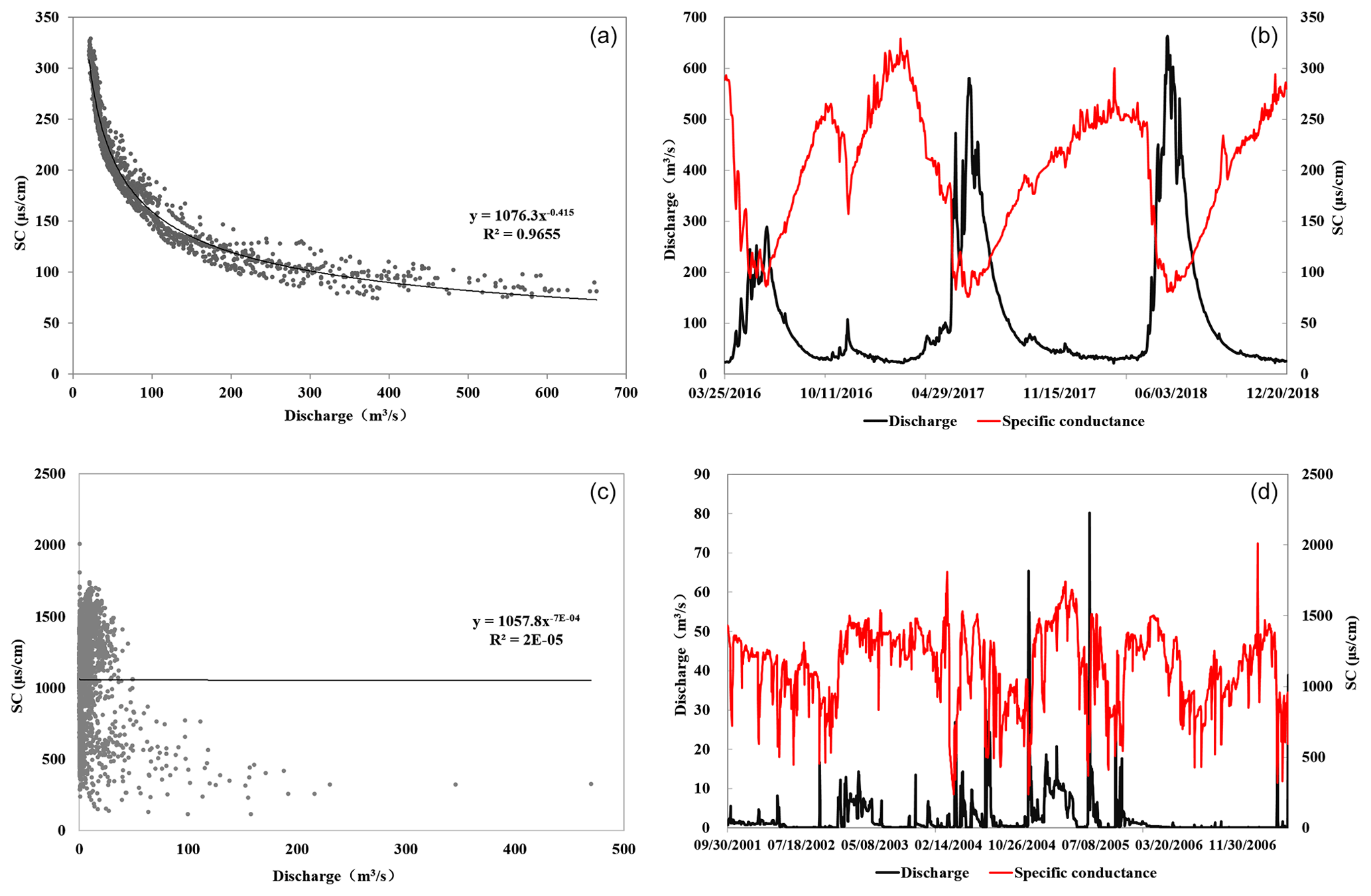
Figure 2Inverse correlation between stream discharge and conductivity (a, c) and their temporal variation (b, d). (a, b) Yellowstone River at Corwin Springs, MT, site no. 06191500. (c, d) North Canadian River below Lake Overholser near Oklahoma City, OK, site no. 07241000.
An analysis of the spatial distribution of inverse correlations between stream discharge and conductivity in the basin showed that the correlations were related to various factors, including topography, altitude, stream discharge and location. In general, most stations located in stream headwater areas with a steep terrain and high elevation showed inverse correlations between flow and conductivity, with 18∕19 of the sites with an elevation above 1500 m showing an . Fewer sites (101∕182) falling within middle and lower reaches with a lower topography showed an (Fig. 3). These results showed that sites with an inverse correlation between conductivity and streamflow were more likely to be located on tributaries than on mainstems. The proportions of sites in which the correlation coefficient for mainstems and tributaries for the Missouri River basin, upper Mississippi River basin, lower Mississippi River basin, and Ohio River basin were 36.4 % (4∕11) and 51.6 % (33∕64), 50 % (3∕6) and 54.5 % (6∕11), 0 % and 77.8 % (14∕18), and 50 % (5∕10) and 70.5 % (31∕44), respectively. On the other hand, the quantitative relationship between streamflow discharge and the correlation coefficient was not significant, and there were significant differences among the stream discharges of sub-basins.

Figure 3Spatial distribution of data analysis points within the Mississippi River basin according to the correlation between conductivity and stream discharge.
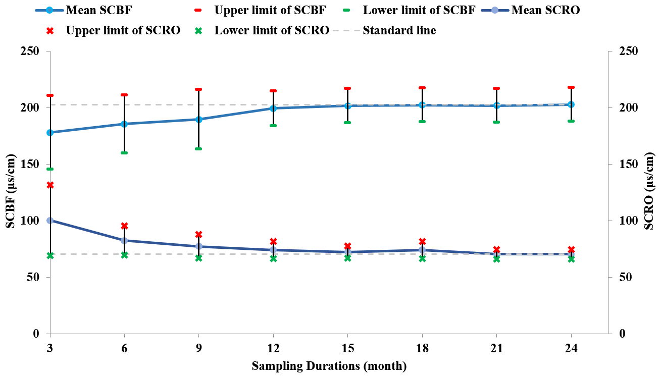
Figure 4Values and variations of SCBF and SCRO with different sampling durations (error bars indicate ±1 SD – 1 standard deviation – for each sampling duration).
3.2 Comparison of different SCBF and SCRO determination methods
The sensitivity analysis results (Table 1) showed that the sensitivity indices of BFI for SCBF and SCRO were all negative, indicating negative correlations between BFI and SCBF (SCRO). The absolute value of the sensitivity index for SCBF was generally greater than that for SCRO, indicating that BFI was affected by SCBF to a greater degree. Taking site 07097000 as an example, uncertainty of 10 % for both SCBF and SCRO resulted in the contribution of SCBF to the uncertainty in BFI being −1.34 times 10 % (−13.4 %), whereas that of SCRO was −0.56 times 10 % (−5.6 %). Therefore, it is clear that more attention should be focused on SCBF to reduce uncertainty in BFI. Furthermore, underestimation or overestimation of SCBF has a different impact on BFI, which will result in overestimation or underestimation of BFI, respectively (Zhang et al., 2013), and it can be proven by Eq. (1) that although underestimation or overestimation of SCBF is of the same degree, the former one has more impact on BFI.
Table 1A comparison of results for different methods used to obtain parameters for baseflow separation methods.
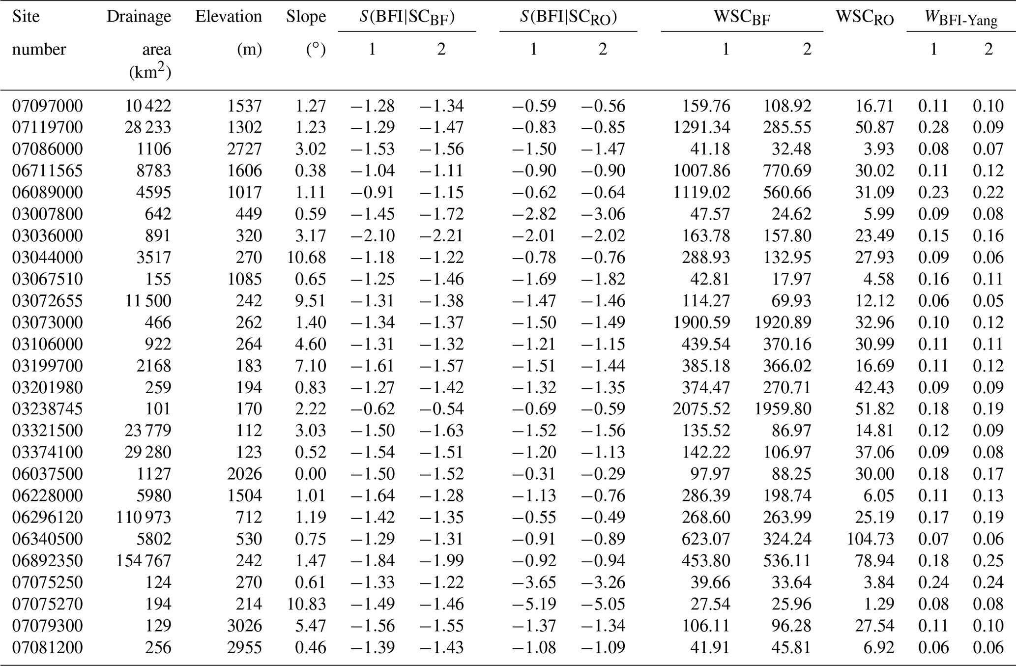
1 and 2 represent yearly dynamic max and yearly dynamic 99th, respectively.
On this basis, the uncertainty values and WBFI-Yang obtained from different determinations of SCBF were compared, with the yearly dynamic maximum and yearly dynamic 99th percentile determination methods mainly considered. This approach was adopted as anthropogenic activities over long periods of time or year-to-year changes in the water table level may result in temporal changes in SCBF (Miller et al., 2014). Therefore, by adopting yearly dynamic maximum and 99th percentile values, the effects of temporal fluctuations in SCBF can be avoided. The results showed that nearly all the uncertainty values and WBFI-Yang obtained from using the yearly dynamic 99th percentile were less than the corresponding values obtained from yearly dynamic maximum values. In addition, the values of were much less than those of , which can be explained by considering that is the standard deviation of the lowest 1 % of measured SC concentrations multiplied by the t value (α=0.05; two-tail). This excluded the possibility of calculating various standard deviations; therefore, various have not been compared in the present study.
3.3 Data requirements for determining SCBF and SCRO
The SCBF, SCRO and BFI values tended to stabilize with increasing sampling duration. In general, with a gradual increase in SCBF, SCRO showed a decreasing trend, whereas BFI showed fluctuation with no significant upward or downward trend (e.g., stream site 07086000 shown in Fig. 4 and other sites shown in Supplement 1). The P values of BFI as determined by the T test did not indicate significant changes with sampling duration, which were greater than 0.05 for durations longer than 3 months. The uncertainty of BFI (i.e., WBFI-Genereux) similarly showed significant variation of as high as 0.31 at a conductivity sampling duration of 3 months but stabilized in the range of 0.14 to 0.27 for sampling duration greater than 3 months (Fig. 5). Therefore, it is clear that a BFI obtained from any continuous data with a sampling duration no longer than 3 months will obviously differ from that obtained from data with a 2-year continuous sampling duration. Therefore, at least 6 months of conductivity records are suggested to obtain reliable estimates of SCBF, SCRO and BFI. Stream sites in which the BFI followed a normal distribution (∼20 stream sites) were assessed, and it was found that there were 10 sites with minimum sampling durations of 3 and 6 months, respectively (see Supplements 1 and 2 for details). Therefore, a minimum of 6-month sampling duration is recommended for application of the CMB method to separate the hydrograph for sites in the Mississippi River basin.
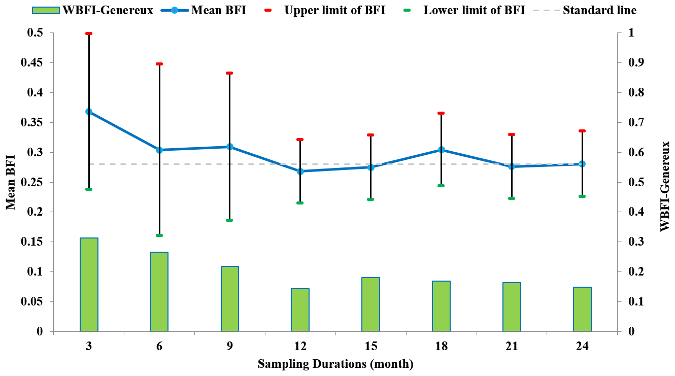
Figure 5Values and variations of mean BFI and WBFI-Genereux with different sampling durations.
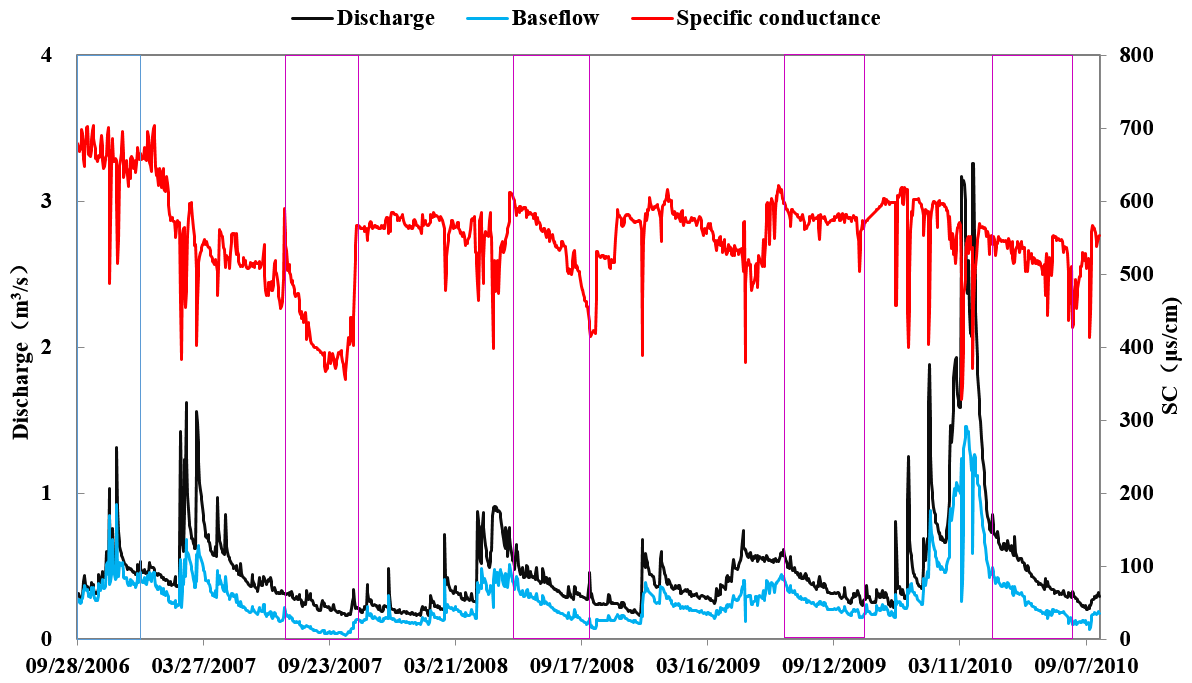
Figure 6Temporal variation in discharge, specific conductance and baseflow for a typical site in the Mississippi River basin.
4.1 Sub-basin characteristics as indicators of the applicability of the CMB method
The results of the present study suggested that the applicability of the CMB method to a particular site can be determined by the presence of an inverse correlation between streamflow discharge and conductivity within monitoring data. Baseflow separation showed unreasonable results for sites in which there was no significant inverse correlation between stream conductivity and discharge. Taking site 01636315 as an example (Fig. 6), an increase in river flow from 28 August to 16 December 2006 was accompanied by a consistently high level of conductivity over the entire monitoring period. The calculated baseflow for this site using Eq. (1) was too large, with a significantly higher ratio during the flood process which clearly did not conform with the mechanism of the baseflow recharge process. During periods of recession (for example, 23 July–6 November 2007, 9 June–24 August 2008, 30 June–21 October 2009, and 23 May–11 August 2010), a gradual decrease in discharge was accompanied by a gradual decrease in conductivity, which is an opposite trend to what would be expected, and resulting in the calculated baseflow hydrograph being significantly lower than the runoff hydrograph. During the dry season, the only source of water in the river was baseflow, and therefore the separation results were clearly incorrect. In fact, for sites in which there was no significant inverse correlation between stream discharge and conductivity, they tended to show a positive relationship. Under these conditions, baseflow separation will generate inaccurate baseflow estimates. Therefore, the present study confirmed the value of an inverse correlation between conductivity and discharge as an indicator of the suitability of the CMB method.
The presence of an inverse correlation between stream conductivity and discharge is dependent on a strong hydraulic connection between groundwater and surface water in a reach and on the major direction of surface water–groundwater interaction being from groundwater to surface water. The CMB method should not be applied to sites in which there is interference in this relationship through anthropogenic activities and other external factors. In this way, conductivity and streamflow data can accurately reflect the natural spatial and temporal variation in baseflow and in the baseflow index. The present study further analyzed the characteristics of factors influencing the inverse correlation between stream conductivity and discharge, including location, topography, surrounding environmental conditions and anthropogenic interferences. By combining the inverse correlation and baseflow separation results, the present study provides a discussion of the key factors influencing the applicability of the CMB method.
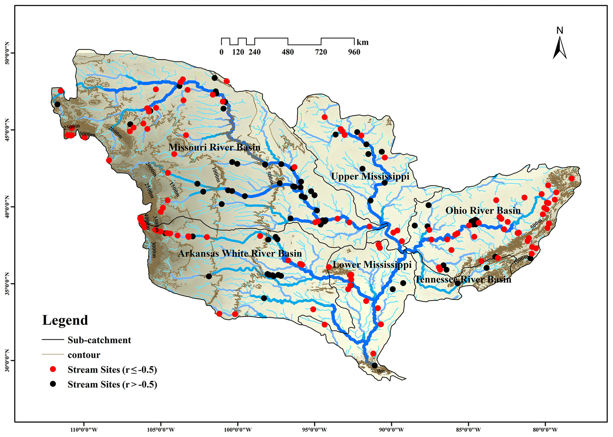
Figure 7Ground elevation and spatial distribution of correlation coefficients for the correlation between stream conductivity and discharge in the Mississippi River basin.
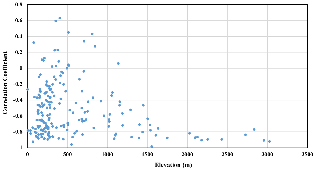
Figure 8Scatterplot of the correlation coefficient against the elevation of the Mississippi River basin monitoring sites.
4.1.1 Impacts of topography and altitude
More than 90 % (18∕19) of the sites located in the upstream area of the basin characterized by a steep terrain and high altitude (particularly those above 1500 m) showed an inverse correlation (i.e., ) between streamflow conductivity and discharge, thereby indicating the good applicability of the CMB method for these sites (Fig. 7). In these areas, high flow velocity and a significant downcutting effect of the river contribute to V-shaped river valleys. There is a strong hydraulic connection between groundwater and surface water in these cases. The middle and lower river reaches are in contrast characterized by lower flow velocity and a weakened downcutting effect, and as the river water level rises, the river may cross a threshold in which it becomes a source of groundwater recharge. This change in relationship between surface water and groundwater results in a breakdown in the inverse correlation between conductivity and discharge, thereby violating the mechanistic understanding the CMB method is based on. In particular, the lower reaches of the basin downstream of Cairo are characterized by a reduced riverbed gradient, wider river valleys and circuitous river channels in which groundwater is recharged by surface water, and the ratio of sites with a medium to high degree of inverse correlation (i.e., ) is reduced to 55 % (101∕182), suggesting that the applicability of the CMB method for these sites is significantly reduced. As shown in Fig. 8, the proportion of sites with a correlation coefficient less than −0.5 increased significantly with increasing site elevation. However, the relationship between the correlation coefficient and site elevation did not strictly satisfy linear inverse correlation, and there are also some sites below 1500 m (especially 500 m) that met the requirements of the correlation coefficient (less than −0.5); these sites were mainly located in the Ohio River basin, the terrain of the basin is relatively flat and the elevation is low. Since the elevations of many sites located in stream headwater areas were less than 500 m, the impact of site location (such as on a tributary or mainstem) may be more significant than elevation.
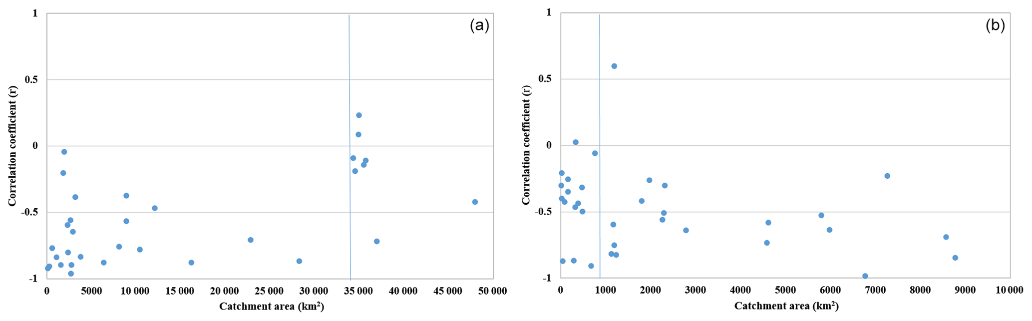
Figure 9Catchment area and correlation coefficient of each site in the Mississippi River basin.
4.1.2 Impacts of site location and streamflow discharge
The present study analyzed and compared site data for the mainstem and tributaries of the Missouri River basin, Arkansas River basin, upper Mississippi River basin and other sub-basins. The results showed that a higher proportion of sites in the tributaries met the requirements of the CMB method. For example, the proportions of tributary and mainstem sites which met the requirements of the CMB method in the Missouri River, Ohio River and upper Mississippi River were 51.6 % and 36.4 %, 70.5 % and 50 %, and 54.5 % and 50 %, respectively. Tributary sites were generally characterized by a high altitude and steep terrain, whereas the mainstem sites fell within plain and low-altitude areas. Therefore, in general, the CMB method is more likely to be applicable to tributary sites.
In theory, streamflow discharge should be a strong determinant of the feasibility of the CMB method. Within a specific watershed, sites with high discharge are mostly located along the mainstems and downstream area, and as discussed above, few are suitable for application of the CMB method. On the other hand, sub-basins with lower flow are likely to be more susceptible to temporal variations in water quantity and the influences of external factors, resulting in distorted results of baseflow separation. However, the results of the present study showed no consistent mathematical relationship between streamflow discharge and correlation coefficient r. Considering the existence of a strong linear relationship between discharge and catchment area for certain sub-basins, for example, for the Missouri River basin in which the R2 of the relationship is 0.94, further analysis of the relationship between catchment area and the applicability of the CMB method was justified. The present study found that the proportion of monitoring sites with a strong inverse correlation coefficient for the stream conductivity–discharge relationship (i.e., ) was relatively low under a very large catchment area. For example, within the Arkansas River basin, only ∼11 % of sites with an area > 34 000 km2 showed a strong inverse correlation coefficient (Fig. 9a). In addition, the proportion of monitoring sites with catchment areas < 800 km2 in which there was a strong inverse correlation coefficient (i.e., ) was relatively low, with approximately 20 % in the Missouri River basin (Fig. 9b). However, it is difficult to simultaneously determine the high-flow and low-flow thresholds for applicability of the CMB method within a particular sub-basin.
4.1.3 Impacts of anthropogenic factors
Human activities can significantly affect stream discharge and water quality, thereby disrupting their natural relationship and invalidating the application of the CMB method. Human activities can result in dramatic changes to river conductivity, and the major impact processes include agricultural irrigation, mining activity, the use of salts as road de-icing agents and groundwater pumping (Kaushal et al., 2005; Crosa et al., 2006; Zume and Tarhule, 2008; Dikio, 2010; Palmer et al., 2010; Bäthe and Coring, 2011; Miguel et al., 2013). Other anthropogenic factors can also result in artificial variations in conductivity, such as industrial wastewater discharge (Piscart et al., 2005; Dikio, 2010), discharge of sewage wastewater (Silva et al., 2000; Williams et al., 2003; Lerotholi et al., 2004) or reduced river discharge due to river impoundment (Mirza, 1998).
Irrigation and the resulting rise in groundwater tables have been reported as one of the main factors leading to significant changes in electrical conductivity of river water, particularly in arid and semi-arid regions in which crop production consumes large quantities of water. Since crops absorb only a fraction of salt introduced through irrigation water, the remaining salt concentrates in the soil, leading to saline soil (Lerotholi et al., 2004). These salts may be leached out through run-off, ultimately ending up in rivers. Therefore, agriculture practices such as fertilizer application can influence the concentrations of conductivity and hence affect the accuracy of the CMB method. In contrast, Li et al. (2018) showed that conductivity of baseflow and surface runoff did not change over time in forest watersheds.
Mining activity is another major source of salts in rivers. Large quantities of potash salts are extracted each year for the manufacture of agricultural fertilizers. During the process of manufacturing of crude salt, which contains not only potash, but also NaCl and other salts, huge amounts of solid residues are stockpiled. The salts are dissolved during precipitation events and may enter surface waters. Mountaintop mining is a mining technique which involves removing 150 or more meters of a mountain to gain access to coal seams and has been blamed for large-scale stream salinization (Pond et al., 2008). The exposure of coal seams to weathering and percolation during coal mining provides many opportunities for the leaching of sulfate from coal wastes into surface waters (Fritz et al., 2010; Bernhardt and Palmer, 2011).
Significant changes in electrical conductivity in the cold regions has often been reported to be the result of the use of salts as road de-icing agents (Löfgren, 2001; Ruth, 2003; Williams et al., 2003). The amount of salts used to de-ice roads in North America increased from 909 000 to 1 347 000 t per winter from 1961 to 1966 (Hanes et al., 1970). During the 1980s, the amount of salts applied to roads increased to 10 million t yr−1 in the United States alone (Salt Institute, 1992). Around 14 million t of salt per year is currently applied to roads in North America (Environment Canada, 2001). The majority of salts used on roads are transported to adjacent streams during rainfall events and snow melting periods (Williams et al., 2003). Consequently, concentrations of salts downstream from major roads have been recorded to be up to 31 times higher than comparative upstream concentrations (Demers and Sage, 1990), and some rural streams have registered chloride concentrations exceeding 0.1 g L−1 (≈0.16 g NaCl g L−1), similar to those found in the salt front of the Hudson River estuary (Kaushal et al., 2005).
Groundwater pumping can reduce groundwater discharge to streams and affect the hydraulic connection between groundwater and surface water and then invalidates the application of the CMB method. When a well is pumped at a constant rate, initially most of the groundwater comes from storage, eventually reaching the river, inducing a leakage of stream water to adjacent aquifer and depleting streamflow significantly (Bredehoeft and Kendy, 2008; Gleeson and Ritcher, 2018). This change in relationship between groundwater and surface water renders CMB method less applicable.
Typically, a monitoring site is located adjacent to a reservoir or other water conservancy infrastructure, which may contribute to significantly increased evaporation and higher conductivity. On the other hand, the reservoir/dam can also provide substantial sources of water in low-flow periods. This may decrease conductivity in streams, thereby undermining the groundwater contribution to streams and leading to an underestimation of baseflow conductivity. In the present study, such affected stream sites included 07130500, 05116000, 06058502, 03400800 and 05370000 located in the upstream part of the Mississippi River basin, and these sites showed relatively poor inverse correlations between stream conductivity and discharge, with correlation coefficients of −0.42, −0.29, 0.06, −0.44 and −0.495, respectively.
Since the Mississippi River basin encompasses almost two-thirds of the entire area of the United States and streamflow occurs through large areas of plain in the Midwest and densely populated areas in the east, the impacts of anthropogenic factors in these areas are great, resulting in limited applicability of the CMB method.
The present study found that, in general, for the entire Mississippi River basin, the CMB method was more applicable for headwater sites, tributaries and high-altitude regions of >1500 m a.s.l. (above sea level), with relatively few impacts by anthropogenic factors. In contrast, the application of the CMB method to downstream flat and low-altitude areas or to areas affected by anthropogenic activities should be carefully considered.
A related study in the upper Colorado River basin suggests higher-elevation watersheds typically have greater baseflow yield (Rumsey et al., 2015), and Dyer (2008) found that high flows in upper streams are mainly stimulated by the snowmelt process and whether the impacts of altitude and site location are mainly due to differences in hydrological regimes, i.e., snow-dominated in upper streams and rain-dominated in lower watersheds. From these findings which are based on the major river basins in North America, we still cannot establish a relationship between hydrological regimes and the applicability of the CMB method. On the other hand, as a large watershed, the Mississippi River basin has sizeable spatial heterogeneity of climate. The role of climate in hydrology, particularly for low flows, is more pronounced in larger watersheds. The influence of hydrological processes on baseflow is complex, particularly when taking climate change into consideration. Therefore, specialized research will be required in the future.
4.2 Optimal method to determine SCBF and SCRO
The comparison of sensitivity analysis results indicated that the influence of parameter SCRO on the separation results was significantly lower than that of parameter SCBF. This result is supported by previous relevant research (Stewart et al., 2007; Zhang et al., 2013; Li et al., 2014; Yang et al., 2019). Moreover, since SCRO represents the minimum conductivity during the wet season, whereas SCBF represents the maximum conductivity during the dry season, the SCRO is less likely to be reduced to an unreasonable extremely low value by the effects of natural or anthropogenic activities. The present study conservatively recommends the 1st percentile of conductivity of the entire monitoring period as indicative of the SCRO to avoid extreme values.

Figure 10Comparison of baseflow calculation results of the main parameter determination methods for a site (07097000) in the Mississippi River basin.
Over a long-term monitoring period, river water quality is often influenced by anthropogenic processes such as release of water from upstream reservoirs and sewage discharge, which can result in extremely high conductivity and underestimated baseflow. The use of the 99th percentile of conductivity as SCBF can effectively avoid these extreme situations. Considering that the climate, human activities and corresponding hydrological processes occurring in a basin will change greatly over the full extent of a monitoring period, it is recommended that the SCBF be determined dynamically to further improve the accuracy of baseflow separation. From the calculated uncertainty results of each method (Table 1), it can be concluded that the uncertainty associated with the use of the dynamic 99th percentile approach was lower than that of the dynamic maximum conductivity approach. Taking site 07097000 as an example for comparing the four approaches of assigning SCRO and SCBF (Fig. 10), during the recession process, the baseflow calculated by the recommended approach appeared rational, whereas the other three approaches generated relatively low baseflow. Therefore, it is suggested that the 1st percentile of conductivity of the entire monitoring period and yearly dynamic 99th percentile approach should be used to determine SCRO and SCBF, respectively.
However, it must be stressed that although the applicability of the CMB method has been verified for a site before determining parameters, it cannot be guaranteed that there will be no anthropogenic disturbance to parameters of a site in which the CMB method has been found to be applicable and that the parameters correspond to the lowest flows very well. For example, leakage of an underground storage tank may last for a long time, which may result in many observations of extremely high conductivities that cannot be avoided by the 99th percentile method. So there is a possibility that the 99th percentile conductivity does not correspond to the lowest flows. Therefore, parameters should be assessed after calculation by the 99th percentile method to further avoid abnormal phenomena and errors within separation results.
4.3 Data requirements for SCBF and SCRO
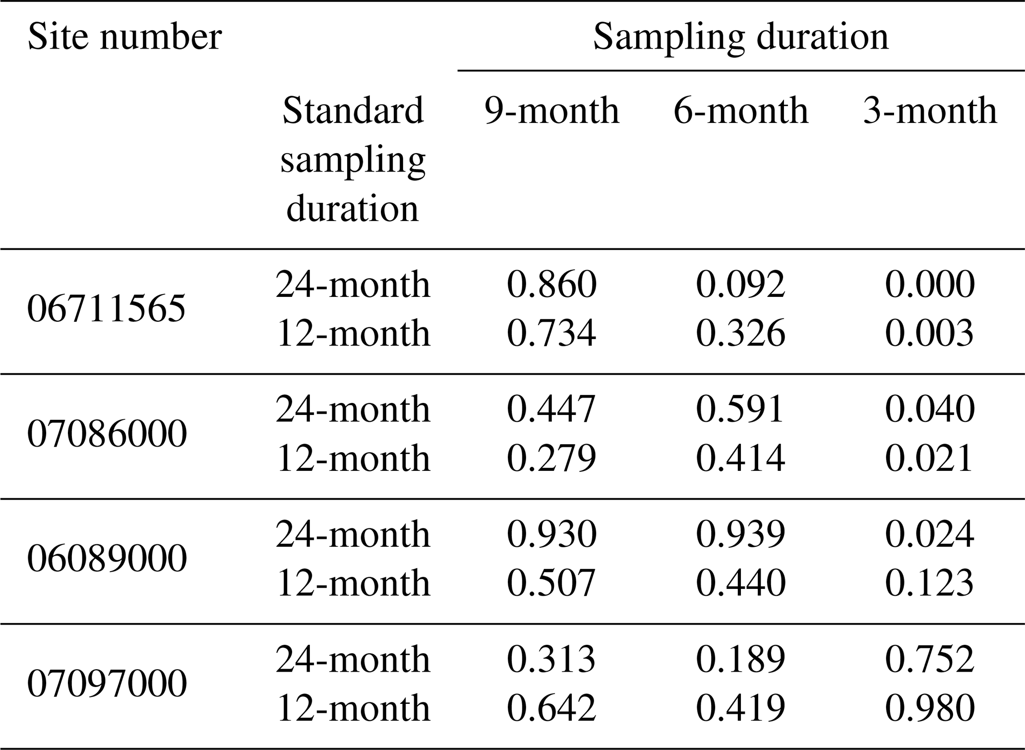
Determining the shortest monitoring periods appropriate for calculating SCRO and SCBF requires determination of the monitoring period required to obtain the reference standard of separation results. Generally, the length of the monitoring period is positively related to the accuracy of the hydrological characteristics of the station reflected by the monitoring data, and the BFI result obtained from a longer monitoring record will be more reasonable compared to that obtained from a relatively shorter record. As an example in the present study and using the BFI calculated by 24 months of data as a standard, the random selection of 20 segments in which no more than half of the data were reused will require monitoring periods of greater than 21 years. For this reason, only 26 of 201 sites were selected for analysis in the present study, from which 5 sites allowed the standard BFI calculation from 24 months of data, whereas the remaining 21 sites allowed the BFI to be calculated from 12 months of data. Therefore, there needs to be further comparison and discussion of the data requirements of utilizing different standard sampling durations. The BFI calculated from 24-month data and yearly data were viewed as a standard for the four stream sites in which the standard sampling durations were 24-months and in which the monitored data followed a normal distribution, respectively. The Student's T test was used to compare differences in BFI obtained from 3, 6 or 9 months of data and the BFI obtained from standard sampling durations (Table 2). The results showed that minimum sampling durations were all less than or equal to 6 months, which indicated that the results obtained by 12-month sampling duration as a standard were also reasonable. Li et al. (2014) similarly questioned their assumption of requiring a dataset of 12-month duration to provide the best representativeness for a watershed and stressed that the uncertainties associated with variations in SCRO and SCBF over years require further study. The results of the present study support their hypothesis that variations in SCRO and SCBF over years will not have a substantial impact on the determination of standard sampling duration.
Table 2Differences between the baseflow index (BFI) obtained from 3, 6, or 9 months of data and the BFI obtained from standard sampling durations.
Through comprehensive qualitative and quantitative analysis of stream discharge and conductivity data for more than 200 hydrological stations in the Mississippi River basin, the present study systematically addressed key questions related to the application of the CMB method to particular sites for baseflow separation. In general, the CMB method was found to be more applicable to tributaries, headwater sites, sites at high altitude and sites with little influence from anthropogenic activities. The applicability of the CMB method can be determined by analyzing the inverse correlation between stream discharge and conductivity. Continuous monitoring of flow and conductivity of longer than 6 months in duration are required to ensure the reliability of baseflow separation results within the CMB method. Within a long series of monitoring data, the 1st percentile method and dynamic 99th percentile method are recommended to determine the parameters of SCRO and SCBF, respectively.
Further study is required to determine which 6 months should be selected for continuous monitoring after the shortest sampling period is determined, as this could be closely related to the geographical location and meteorological conditions of each station. In addition, future research should address whether monitoring should occur during the wet season, dry season, or both. Future research should also consider large watersheds in other latitudes and climates so as to compare and verify the conclusions of the present study and to establish more generalized methods. The present study can act as a reference for the identification of parameters of baseflow separation methods so as to improve the accuracy of these methods.
All streamflow and conductivity data can be retrieved from the US Geological Survey's (USGS) National Water Information System (NWIS) website using the special site number: http://waterdata.usgs.gov/nwis (last access: 10 March 2019) (NWIS, 2019).
The supplement related to this article is available online at: https://doi.org/10.5194/hess-24-6075-2020-supplement.
HL developed the research train of thought. CX completed the data requirement analysis. JZ carried out the CMB method suitability assessment. BL compared different parameter determination methods. HL prepared the manuscript with contributions from all the coauthors.
The authors declare that they have no conflict of interest.
This work is supported by the project funded by the National Key R & D Program of China (2018YFC0406503) and the National Natural Science Foundation of China (U19A20107, 41702252) special funds for basic scientific research-operating expenses of central universities. We would like to express our sincere thanks to the editor and the anonymous reviewers for the constructive and positive advice and comments which helped improve the manuscript.
This research has been supported by the National Key R & D Program of China (grant no. 2018YFC0406503), the National Natural Science Foundation of China (grant nos. U19A20107 and 41702252), and special funds for basic scientific research-operating expenses of central universities (grant no. 202010).
This paper was edited by Stacey Archfield and reviewed by two anonymous referees.
Arnold, J. G. and Allen, P. M.: Automated methods for estimating baseflow and ground water recharge from streamflow records, J. Am. Water Resour. Assoc., 35, 411–424, https://doi.org/10.1111/j.1752-1688.1999.tb03599.x, 1999.
Arnold, J. G., Allen, P. M., Muttiah, R., and Bernhardt, G.: Automated Base Flow Separation and Recession Analysis Techniques, Ground Water, 33, 1010–1018, https://doi.org/10.1111/j.1745-6584.1995.tb00046.x, 1995.
Arnold, J. G., and Allen, P. M.: Automated Methods For Estimating Baseflow And Ground Water Recharge From Streamflow Records, J. Am. Water Resour. Assoc., 35, 411–424, https://doi.org/10.1111/j.1752-1688.1999.tb03599.x, 1999.
Arnold, J. G., Muttiah, R. S., Srinivasan, R., and Allen, P. M.: Regional estimation of base flow and groundwater recharge in the Upper Mississippi river basin, J. Hydrol., 227, 21–40, https://doi.org/10.1016/s0022-1694(99)00139-0, 2000.
Bäthe, J. and Coring, E.: Biological effects of anthropogenic salt-load on the aquatic Fauna: A synthesis of 17 years of biological survey on the rivers Werra and Weser, Limnologica, 41, 125–133, https://doi.org/10.1016/j.limno.2010.07.005, 2011.
Bernhardt, E. S. and Palmer, M. A.: The environmental costs of mountaintop mining valley fill operations for aquatic ecosystems of the Central Appalachians, in: Annals of the New York Academy of Sciences, Blackwell Publishing Inc., 39–57, https://doi.org/10.1111/j.1749-6632.2011.05986.x, 2011.
Bredehoeft, J. and Kendy, E.: Strategies for offsetting seasonal impacts of pumping on a nearby stream, Ground Water, 46, 23–29, https://doi.org/10.1111/j.1745-6584.2007.00367.x, 2008.
Caissie, D., Pollock, T. L., and Cunjak, R. A.: Variation in stream water chemistry and hydrograph separation in a small drainage basin, J. Hydrol., 178, 137–157, https://doi.org/10.1016/0022-1694(95)02806-4, 1996.
Cey, E. E., Rudolph, D. L., Parkin, G. W., and Aravena, R.: Quantifying groundwater discharge to a small perennial stream in southern Ontario, Canada, J. Hydrol., 210, 21–37, https://doi.org/10.1016/s0022-1694(98)00172-3, 1998.
Covino, T. P. and McGlynn, B. L.: Stream gains and losses across a mountain-to-valley transition: Impacts on watershed hydrology and stream water chemistry, Water Resour. Res., 43, 2457–2463, https://doi.org/10.1029/2006wr005544, 2007.
Crosa, G., Froebrich, J., Nikolayenko, V., Stefani, F., Galli, P., and Calamari, D.: Spatial and seasonal variations in the water quality of the Amu Darya River (Central Asia), Water Res., 40, 2237–2245, https://doi.org/10.1016/j.watres.2006.04.004, 2006.
Demers, C. L. and Sage Jr., R. W.: Effects of road deicing salt on chloride levels in four adirondack streams, Water Air Soil Pollut., 49, 369–373, https://doi.org/10.1007/BF00507076, 1990.
Dhakal, N., Fang, X., Cleveland, T. G., Thompson, D. B., Asquith, W. H., and Marzen, L. J.: Estimation of Volumetric Runoff Coefficients for Texas Watersheds Using Land-Use and Rainfall-Runoff Data, J. Irrig. Drain. Eng., 138, 43–54, https://doi.org/10.1061/(asce)ir.1943-4774.0000368, 2012.
Dikio, E. D.: Water quality evaluation of Vaal River, Sharpeville and Bedworth Lakes in the Vaal region of South Africa, Res. J. Appl. Sci. Eng. Technol., 2, 574–579, 2010.
Dyer, J.: Snow depth and streamflow relationships in large North American watersheds, J. Geophys. Res.-Atmos., 113, D18113, https://doi.org/10.1029/2008JD010031, 2008.
Eckhardt, K.: A comparison of baseflow indices, which were calculated with seven different baseflow separation methods, J. Hydrol., 352, 168–173, https://doi.org/10.1016/j.jhydrol.2008.01.005, 2008.
Environment Canada: Canadian Environmental Protection Act, 1999, Priority Substances List Assessment Report e Road Salt, Hull, Quebec, 2001.
Fritz, K. M., Fulton, S., Johnson, B. R., Barton, C. D., Jack, J. D., Word, D. A., and Burke, R. A.: Structural and functional characteristics of natural and constructed channels draining a reclaimed mountaintop removal and valley fill coal mine, J. N. Am. Benthol. Soc., 29, 673–689, https://doi.org/10.1899/09-060.1, 2010.
Furey, P. R. and Gupta, V. K.: A physically based filter for separating base flow from streamflow time series, Water Resour. Res., 37, 2709–2722, https://doi.org/10.1029/2001wr000243, 2001.
Genereux, D. P. and Hooper, R. P.: Oxygen and Hydrogen Isotopes in Rainfall-Runoff Studies, in: Isotope Tracers in Catchment Hydrology, Elsevier, Amsterdam, 319–346, 1998.
Gleeson, T. and Richter, B.: How much groundwater can we pump and protect environmental flows through time? Presumptive standards for conjunctive management of aquifers and rivers, River Res. Appl., 34, 83-92, 10.1002/rra.3185, 2018.
Hanes, R. E., Zelazny, L. W., and Blaser, R. E.: Effects of Deicing Salts on Water Quality and Biota: Literature Review and Recommended Research, National Cooperative Highway Research Program Report 91, Highway Research Board, National Research Council, Washington, D.C., 1970.
Heppell, C. M. and Chapman, A. S.: Analysis of a two-component hydrograph separation model to predict herbicide runoff in drained soils, Agr. Water Manage., 79, 177–207, https://doi.org/10.1016/j.agwat.2005.02.008, 2006.
Hewlett, J. D. and Hibbert, A. R.: Factors affecting the response of small watersheds to precipitation in humid areas, Forest Hydrol., 1, 275–290, 1967.
Huyck, A. A. O., Pauwels, V. R. N., and Verhoest, N. E. C.: A base flow separation algorithm based on the linearized Boussinesq equation for complex hillslopes, Water Resour. Res., 41, 553–559, https://doi.org/10.1029/2004wr003789, 2005.
Kaushal, S. S., Groffman, P. M., Likens, G. E., Belt, K. T., Stack, W. P., Kelly, V. R., Band, L. E., and Fisher, G. T.: Increased salinization of fresh water in the northeastern United States, P. Natl. Acad. Sci. USA, 102, 13517–13520, https://doi.org/10.1073/pnas.0506414102, 2005.
Kendall, C. and McDonnell, J. J.: Isotope tracers in catchment hydrology, Elsevier, Amsterdam, 2012.
Kunkle, G. R.: Computation of ground-water discharge to streams during floods, or to individual reaches during base flow, by use of specific conductance, US Geol. Surv. Prof. Pap. 207-210, US Geological Survey, Reston, VA, USA, 1965.
Lerotholi, S., Palmer, C. G., and Rowntree, K.: Bioassessment of a River in a Semiarid, Agricultural Catchment, Eastern Cape, in: Proceedings of the 2004 Water Institute of Southern Africa (WISA) Biennial Conference, 2–6 May 2004, Cape Town, South Africa, 338–344, 2004.
Li, Q., Xing, Z., Danielescu, S., Li, S., Jiang, Y., and Meng, F.-R.: Data requirements for using combined conductivity mass balance and recursive digital filter method to estimate groundwater recharge in a small watershed, New Brunswick, Canada, J. Hydrol., 511, 658–664, https://doi.org/10.1016/j.jhydrol.2014.01.073, 2014.
Li, Q., Wei, X. H., Zhang, M. F., Liu, W. F., Giles-Hansen, K., and Wang, Y.: The cumulative effects of forest disturbance and climate variability on streamflow components in a large forest-dominated watershed, J. Hydrol., 557, 448–459, https://doi.org/10.1016/j.jhydrol.2017.12.056, 2018.
Lo, E.: Gaussian error propagation applied to ecological data: Post-ice-storm-downed woody biomass, Ecol. Monogr., 75, 451–466, https://doi.org/10.1890/05-0030, 2005.
Löfgren, S.: The chemical effects of deicing salt on soil and stream water of five catchments in southeast Sweden, Water Air Soil Pollut., 130, 863–868, https://doi.org/10.1023/A:1013895215558, 2001.
Lott, D. A. and Stewart, M. T.: A Power Function Method for Estimating Base Flow, Ground Water, 51, 442–451, https://doi.org/10.1111/j.1745-6584.2012.00980.x, 2012.
Lott, D. A. and Stewart, M. T.: Base flow separation: A comparison of analytical and mass balance methods, J. Hydrol., 535, 525–533, https://doi.org/10.1016/j.jhydrol.2016.01.063, 2016.
Matsubayashi, U., Velasquez, G. T., and Takagi, F.: Hydrograph separation and flow analysis by specific electrical conductance of water, J. Hydrol., 152, 179–199, https://doi.org/10.1016/0022-1694(93)90145-y, 1993.
Miguel, C. A., Kefford, B. J., Piscart, C., Prat, N., Schaefer, R. B., and Schulz, C.-J.: Salinisation of rivers: An urgent ecological issue, Environ. Pollut., 173, 157–167, https://doi.org/10.1016/j.envpol.2012.10.011, 2013.
Miller, M. P., Susong, D. D., Shope, C. L., Heilweil, V. M., and Stolp, B. J.: Continuous estimation of baseflow in snowmelt-dominated streams and rivers in the Upper Colorado River Basin: A chemical hydrograph separation approach, Water Resour. Res., 50, 6986–6999, https://doi.org/10.1002/2013wr014939, 2014.
Mirza, M.: Diversion of the Ganges Water at Farakka and Its Effects on Salinity in Bangladesh, Environ. Manage., 22, 711–722, https://doi.org/10.1007/s002679900141, 1998.
Nakamura, R.: Runoff analysis by electrical conductance of water, J. Hydrol., 14, 197–212, https://doi.org/10.1016/0022-1694(71)90035-7, 1971.
Nathan, R. J. and McMahon, T. A.: Evaluation of automated techniques for base flow and recession analyses, Water Resour. Res., 26, 1465–1473, https://doi.org/10.1029/wr026i007p01465, 1990.
NWIS: US Geological Survey's National Water Information System, available at: http://waterdata.usgs.gov/nwis, last access: 10 March 2019.
Palmer, M. A., Bernhardt, E. S., Schlesinger, W. H., Eshleman, K. N., Foufoula-Georgiou, E., Hendryx, M. S., Lemly, A. D., Likens, G. E., Loucks, O. L., Power, M. E., White, P. S., and Wilcock, P. R.: Mountaintop Mining Consequences, Science, 327, 148–149, https://doi.org/10.1126/science.1180543, 2010.
Pellerin, B. A., Wollheim, W. M., Feng, X., and Vörösmarty, C. J.: The application of electrical conductivity as a tracer for hydrograph separation in urban catchments, Hydrol. Process., 22, 1810–1818, https://doi.org/10.1002/hyp.6786, 2008.
Pinder, G. F. and Jones, J. F.: Determination of the ground-water component of peak discharge from the chemistry of total runoff, Water Resour. Res., 5, 438–445, https://doi.org/10.1029/wr005i002p00438, 1969.
Piscart, C., Moreteau, J. C., and Beisel, J. N.: Biodiversity and structure of macroinvertebrate communities along a small permanent salinity gradient (Meurthe River, France), Hydrobiologia, 551, 227–236, https://doi.org/10.1007/s10750-005-4463-0, 2005.
Pond, G. J., Passmore, M. E., Borsuk, F. A., Reynolds, L., and Rose, C. J.: Downstream effects of mountaintop coal mining: Comparing biological conditions using family- and genus-level macroinvertebrate bioassessment tools, J. N. Am. Benthol. Soc., 27, 717–737, https://doi.org/10.1899/08-015.1, 2008.
Ran, Q., Su, D., Li, P., and He, Z.: Experimental study of the impact of rainfall characteristics on runoff generation and soil erosion, J. Hydrol., 424–425, 99–111, https://doi.org/10.1016/j.jhydrol.2011.12.035, 2012.
Rosenberry, D. O. and Winter, T. C.: Dynamics of water-table fluctuations in an upland between two prairie-pothole wetlands in North Dakota, J. Hydrol., 191, 266–289, https://doi.org/10.1016/s0022-1694(96)03050-8, 1997.
Rumsey, C. A., Miller, M. P., Susong, D. D., Tillman, F. D., and Anning, D. W.: Regional scale estimates of baseflow and factors influencing baseflow in the Upper Colorado River Basin, J. Hydrol. Reg. Stud., 4, 91–107, https://doi.org/10.1016/j.ejrh.2015.04.008, 2015.
Ruth, O.: The effects of de-icing in Helsinki urban streams, Southern Finland, Water Sci. Technol., 48, 33–43, https://doi.org/10.2166/wst.2003.0486, 2003.
Salt Institute: Deicing Salt Factsd (A Quick Reference), Salt Institute, Alexandria, VA, 1992.
Sanford, W. E., Nelms, D. L., Pope, J. P., and Selnick, D. L.: Quantifying components of the hydrologic cycle in Virginia using chemical hydrograph separation and multiple regression analysis, US Geological Survey Scientific Investigations Report 5198, US Geological Survey, Reston, VA, USA, 152 pp., 2011.
Silva, E. I. L., Shimizu, A., and Matsunami, H.: Salt pollution in a Japanese stream and its effects on water chemistry and epilithic algal chlorophyll-a, Hydrobiologia, 437, 139–148, https://doi.org/10.1023/a:1026598723329, 2000.
Stewart, M., Cimino, J., and Ross, M.: Calibration of Base Flow Separation Methods with Streamflow Conductivity, Ground Water, 45, 17–27, https://doi.org/10.1111/j.1745-6584.2006.00263.x, 2007.
Tan, S. B., Lo, E. Y.-M., Shuy, E. B., Chua, L. H., and Lim, W. H.: Hydrograph Separation and Development of Empirical Relationships Using Single-Parameter Digital Filters, J. Hydrol. Eng., 14, 271–279, https://doi.org/10.1061/(asce)1084-0699(2009)14:3(271), 2009.
Williams, M. L., Palmer, C. G., and Gordon, A. K.: Riverine macroinvertebrate responses to chlorine and chlorinated sewage effluents – Acute chlorine tolerances of Baetis harrisoni (Ephemeroptera) from two rivers in KwaZulu-Natal, South Africa, Water SA, 29, 483–488, https://doi.org/10.4314/wsa.v29i4.5056, 2003.
Yang, W., Xiao, C., and Liang, X.: Technical note: Analytical sensitivity analysis and uncertainty estimation of baseflow index calculated by a two-component hydrograph separation method with conductivity as a tracer, Hydrol. Earth Syst. Sci., 23, 1103–1112, https://doi.org/10.5194/hess-23-1103-2019, 2019.
Zhang, R., Li, Q., Chow, T. L., Li, S., and Danielescu, S.: Baseflow separation in a small watershed in New Brunswick, Canada, using a recursive digital filter calibrated with the conductivity mass balance method, Hydrol. Process., 27, 2659–2665, https://doi.org/10.1002/hyp.9417, 2013.
Zume, J. and Tarhule, A.: Simulating the impacts of groundwater pumping on stream-aquifer dynamics in semiarid northwestern Oklahoma, USA, Hydrogeol. J., 16, 797–810, https://doi.org/10.1007/s10040-007-0268-8, 2008.