the Creative Commons Attribution 4.0 License.
the Creative Commons Attribution 4.0 License.
 | 18 Dec 2020
Assessing the capabilities of the Surface Water and Ocean Topography (SWOT) mission for large lake water surface elevation monitoring under different wind conditions
Jean Bergeron
Gabriela Siles
Robert Leconte
Mélanie Trudel
Damien Desroches
Daniel L. Peters
Lakes are important sources of freshwater and provide essential ecosystem services. Monitoring their spatial and temporal variability, and their functions, is an important task within the development of sustainable water management strategies. The Surface Water and Ocean Topography (SWOT) mission will provide continuous information on the dynamics of continental (rivers, lakes, wetlands and reservoirs) and ocean water bodies. This work aims to contribute to the international effort evaluating the SWOT satellite (2022 launch) performance for water balance assessment over large lakes (e.g., >100 km2). For this purpose, a hydrodynamic model was set up over Mamawi Lake, Canada, and different wind scenarios on lake hydrodynamics were simulated. The derived water surface elevations (WSEs) were compared to synthetic elevations produced by the Jet Propulsion Laboratory (JPL) SWOT high resolution (SWOT-HR) simulator. Moreover, water storages and net flows were retrieved from different possible SWOT orbital configurations and synthetic gauge measurements. In general, a good agreement was found between the WSE simulated from the model and those mimicked by the SWOT-HR simulator. Depending on the wind scenario, errors ranged between approximately −2 and 5 cm for mean error and from 30 to 70 cm root mean square error. Low spatial coverage of the lake was found to generate important biases in the retrievals of water volume or net flow between two satellite passes in the presence of local heterogeneities in WSE. However, the precision of retrievals was found to increase as spatial coverage increases, becoming more reliable than the retrievals from three synthetic gauges when spatial coverage approaches 100 %, demonstrating the capabilities of the future SWOT mission in monitoring dynamic WSE for large lakes across Canada.
- Article
(9462 KB) - Full-text XML
- BibTeX
- EndNote


The works published in this journal are distributed under the Creative Commons Attribution 4.0 License. This license does not affect the Crown copyright work, which is re-usable under the Open Government Licence (OGL). The Creative Commons Attribution 4.0 License and the OGL are interoperable and do not conflict with, reduce or limit each other.
© Crown copyright 2020
Inland freshwater systems (e.g., rivers, lakes, ponds and wetlands) are important sources for society and provide essential habitat to sustain biodiversity and valuable ecosystem services (e.g., Palmer et al., 2015). As part of the hydrological cycle, the extent and volume of water stored on the landscape changes through time which, according to the water budget equation, depends on inflow (precipitation, overland runoff and groundwater) and outflow (evaporation, seepage, withdrawals to satisfy residential, agriculture and industrial demands and streamflow) components. Temporal monitoring of continental waters is important for assessing trends of and variability in their availability in a changing climate (e.g., Frasson et al., 2017; Bonsal et al., 2019) and to support programs for the mitigation of hydro hazards (e.g., drought and flooding; Rahman and Di, 2017). Hydrometric stations can provide useful information for water management endeavours (e.g., water levels and discharge). However, as stated in previous studies, the available network of gauges is spatially insufficient for the surveillance of global rivers and lakes (e.g., Pavelsky et al., 2014). Densifying this ground-based monitoring system would be costly and challenging to install and maintain in difficult-to-access areas due their remote location and/or in zones affected by political or other conflicts (wars and internationally shared water bodies; e.g., Gleason and Hamdan, 2017). Moreover, local measurement systems can present technical problems that translate into important gaps in the recorded time series. For example, extensive areas of the North America and Eurasia are affected by spring ice breakup events that can disrupt monitoring until the gauge is reset. Remote sensing technologies and methods offer the possibility to complement and enhance in situ observations, providing valuable spatially distributed information on ungauged water systems (e.g., da Silva et al., 2014). Delineation of and changes in surface water area for river, wetland and lake systems have been successfully achieved via the application of optical (e.g., Gardelle et al., 2010; Jiang et al., 2014), radar (e.g., Ding and Li, 2011; Zeng et al., 2017) and a combination of satellite imagery (e.g., Töyra et al., 2002; Bwangoy et al., 2010; Bioresita et al., 2019). The estimation of other important hydrological variables such as water level, discharge, water volume and their variations can represent a more difficult challenge (Grippa et al., 2019). This challenge has been addressed by exploiting information acquired by radar and laser altimetry (e.g., Maheu et al., 2003; Crétaux and Birkett, 2006). For example, da Silva et al. (2012) used EnviSat Radar Altimeter 2 (RA-2) data to characterize water storage in rivers, floodplains, wetlands and lakes in the Amazon basin. Internationally, estimations of changes in lake and reservoir volume have been attempted by exploiting different satellite altimetry databases including both laser (Ice, Clouds, and Land Elevation Satellite – ICEsat 1) and radar data (TOPEX/Poseidon, Jason-1, Jason-2 and EnviSat; e.g., Duan and Bastiaanssen, 2013; Crétaux et al., 2016). In Canada, Interferometric Synthetic Aperture Radar (InSAR) has been employed to estimate relative water level changes for lakes and wetlands (e.g., Mohammadimanesh et al., 2018; Siles et al., 2020). Musa et al. (2015) present a review of hydrological applications using optical, radar imagery and altimetric data.
Despite the demonstrated potential of current radar altimetry satellite missions, the large footprint dimension (a few hundred metres to several kilometres) makes the detection of water levels for small water bodies difficult (e.g., Grippa et al., 2019). For example, in order to detect the water level over a given lake, the strong backscatter signal coming from several surrounding elements (nearby wetlands, small lakes, rivers, wet outcrops and sands) needs to be discriminated and removed from the measured waveform, otherwise it may not be possible to measure water levels from the target water body. ICEsat 1 and 2 laser sensors provide a better ground track spatial resolution, allowing us to partially overcome limitations of the radar sensors (e.g. Wang et al., 2011). However, the presence of clouds and other atmospheric effects reduce the accuracy of the laser-based sensors (Brenner et al., 2007). In addition, the ground separation between successive tracks are, generally, very large (several kilometres), and their revisit time can be infrequent (up to 35 d), which could limit the spatial and temporal information over a considered surface water feature. Some studies have successfully combined synthetic aperture radar (SAR) imagery and radar altimetry in order to overcome these constraints and to provide high-resolution water levels (e.g., Baup et al., 2014) and water level changes (e.g., Kim et al., 2009). Despite the performance of those approaches, it remains difficult to find altimetric data, radar and optical imagery acquired at the same time or within a few days' difference for a given watercourse and body.
The Surface Water and Ocean Topography (SWOT) satellite mission, expected to be launched in 2022, is the first satellite of its type comprised of a bistatic near-nadir SAR interferometer that will enable us to benefit from the combined advantages of radar altimeters (water level detection) and SAR imagery (high spatial resolution). This mission is a cooperation between NASA and the Centre National d'Études Spatiales (CNES), with collaboration of the Canadian Space Agency (CSA) and the United Kingdom Space Agency (e.g., Biancamaria et al., 2016). This Ka-band satellite will map water surface elevation (WSE) and water surface slope (WSS) along rivers and lakes around the globe, with SWOT-derived subproducts, such as river discharge and lake water volume change (e.g., Biancamaria et al., 2016). Measurements from this satellite cover water surfaces (rivers wider than 100 m and lakes/reservoirs with a minimum surface area of 250 m × 250 m), located between 78∘ S and 78∘ N, with a revisit time of 21 d (Pavelsky et al., 2014). Due to the polar orbit of the satellite, lakes in higher latitudes will likely benefit from multiple coverages per 21 d cycle.
Most published studies on SWOT capabilities have focused on its potential for river applications. For example, by studying the impact of different river reach definition strategies on discharge estimation (Frasson et al., 2017), river depth assimilation (Häfliger et al., 2019) and river bathymetry definition (Yoon et al., 2012), among other applications (e.g., Garambois and Monnier, 2015; Gleason et al., 2014; Domeneghetti et al., 2018; Oubanas et al., 2018). Only a few studies have been found in the literature that focused on the performance of SWOT over lakes and reservoirs. Munier et al. (2015) evaluated the effect of SWOT data assimilation on reservoirs, showing that it can contribute to improving the management of the Sélingué Dam in the Niger River Basin, Mali, to meet environmental constraints. Solander et al. (2016) presented a characterization and estimation of errors that could affect SWOT observations on artificial reservoirs. Recently, Grippa et al. (2019) showed the potential of SWOT for monitoring the seasonal variability in water levels and volume in small lakes of the central Sahel, Africa.
Environmental factors, such as wind, can have a notable influence on the spatial distribution of water levels in large water bodies (e.g., lakes and oceans). For instance, high sustained winds from one direction can push the water to one end of the lake and drop at the opposite end. Such a phenomenon, known as a seiche, resulted in surges reaching up to 3 m in more extreme cases in Lake Erie, eastern Canada (Farhadzadeh et al., 2017). In western Canada, wind seiches on Lake Athabasca have been observed, leading to vertical water fluctuations up to 1 m and pushing water into adjacent connected lakes (e.g., Mamawi Lake) of the Peace–Athabasca delta (Timoney, 2013). The potential impacts of such wind-generated episodic events on SWOT observations thus require investigation and understanding prior to mission launch.
To support the mission, the SWOT Canada Terrestrial Hydrology (SWOT-C TH) team has developed several research field- and modelling-based projects (Pietroniro et al., 2019). One of these projects is focused on the Peace–Athabasca delta (PAD) in northern Alberta, Canada. In support of the international effort, the main goal of the following SWOT-C TH work is to assess the capability of SWOT to quantify lake water volume changes for a large lake under different wind scenarios. Specifically, the objective is to set up a hydrodynamic model over Mamawi Lake, located at the centre of the PAD in order to (i) evaluate WSE, as mimicked by the SWOT high-resolution (HR) simulator, to those provided by a hydrodynamic model and in situ lake gauges and (ii) estimate water storages retrieved from different possible SWOT orbital pass coverage over the lake.
The Peace–Athabasca delta (PAD; ∼ 60 000 km2) is a Ramsar wetland site of international importance located in northern Alberta, Canada, where the Peace and Athabasca rivers converge at the western end of Lake Athabasca (∼ 7800 km2). The majority of the delta (80 %) is located within the Wood Buffalo National Park, which is a United Nations Educational, Scientific and Cultural Organization (UNESCO) World Heritage Site. The PAD encompass several large, relatively shallow, interconnected lakes (Lake Claire, Mamawi Lake and Richardson Lake) and more than 1000 smaller lakes and wetlands that have varying hydraulic connectivity to the main flow system, depending on elevation and distance inland (Peters et al., 2006a, b). The perched lakes and wetlands of the delta provide important ecosystem services and are dependent on occasional floodwater input from ice jam and open-water flood events to maintain aquatic conditions. Climate variability and change, river regulation and water use in upstream basin areas influence wetting and drying phases of the delta, which in turn influence local species, ecological functions and integrity (e.g., Beltaos, 2014; Ward and Gorelick, 2018; Bush et al., 2020).
At the heart of the PAD is Mamawi Lake (∼ 200 km2 and <3 m depth). This lake is directly connected to Lake Claire through the Prairie River and Lake Athabasca through the Chenal des Quatre Fourches (Fig. 1). A major source of water inflow is the Athabasca River, and the outflow is normally northward towards the Slave River, but it can reverse direction when the stage on the Peace River is higher than the central lakes, occasionally leading to extremely high lake levels that expand beyond the shoreline (Leconte et al., 2001; Peters and Buttle, 2010). Mamawi Lake is also prone to a short-term rise/fall in water levels due to wind-driven seiche events. Periodic seiches can move water into low-lying basins and expose mudflats, the dynamics of which is poorly understood (Timoney, 2013).
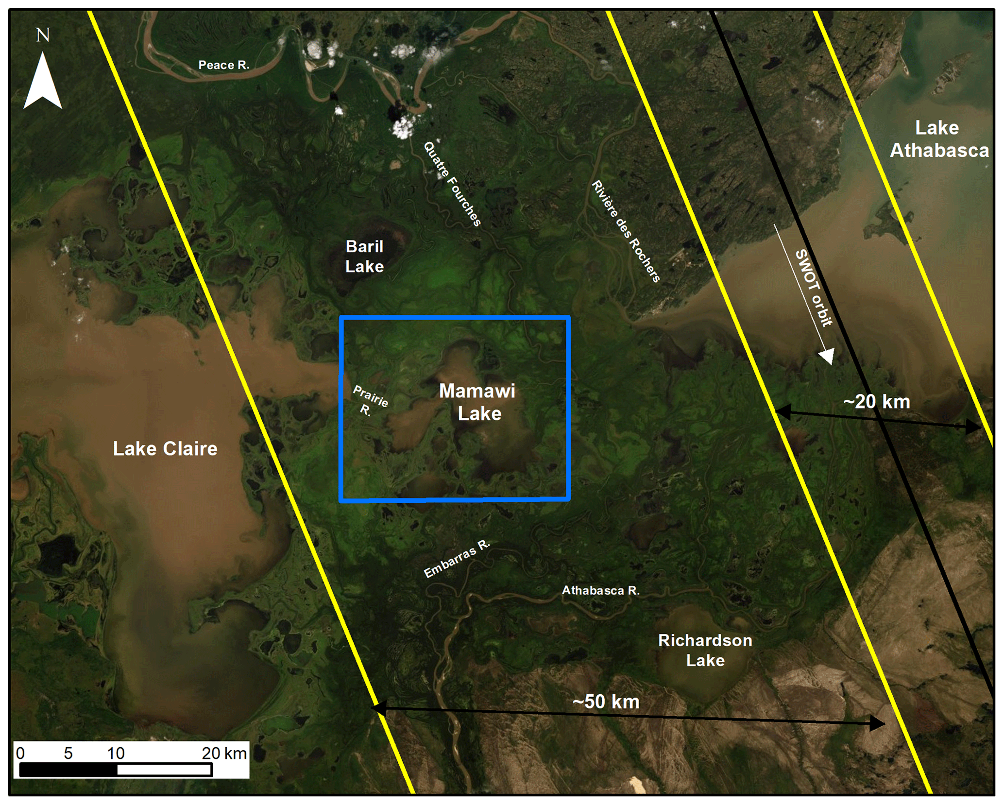
Figure 1Mamawi Lake (blue rectangle) and other main lakes and rivers within the Peace–Athabasca delta. The Surface Water and Ocean Topography (SWOT) orbital pass 303 over the area of study is depicted. The satellite nadir track is indicated by the black line, and the satellite swath is (∼ 50 km) delimited by the yellow lines. Base map source: Esri, DigitalGlobe, GeoEye, Earthstar Geographics, National Centre for Space Studies (CNES) and Airbus Defence and Space, United States Department of Agriculture (USDA), United States Geological Survey (USGS), AeroGRID, Institut Geographique National (IGN), and the GIS User Community.
The PAD receives continental arctic and maritime arctic air masses during the winter, whereas maritime polar winds are common in the summer; northwesterly winds predominate for most of the year (Phillips, 1990). The continental climate triggers a wide variation in climatological variables between the winter and the summer (Phillips, 1990). Temperatures in the area typically vary between <−20 and >20 ∘C, with the highest temperature occurring during the month of July and the lowest during the month of January (Peters et al., 2006a). The largest precipitations occur in the midsummer and the lowest amounts are usually at the end of winter (Peters et al., 2006a).
A number of extensive ground-based and remotely sensed derived data sets are required to set up a hydrodynamic model and to perform the SWOT simulations. As part of the SWOT-C TH effort (Pietroniro et al., 2019), two fieldwork campaigns were carried out in the PAD during summer 2017 by the Environment and Climate Change Canada and the University of Sherbrooke with support from Wood Buffalo National Parks. In addition to the long-term water level hydrometric network stations on the Prairie River and Mamawi Lake outflow, project-specific measurements of water levels and streamflow were also taken in the main channels around Mamawi Lake (see Fig. 2). The bathymetry of the lake and channel cross sections was acquired by a combination of weighted line depth and echo-sounding measurements. These data were used to define the boundary conditions and develop the hydrodynamic model (see Sect. 4).
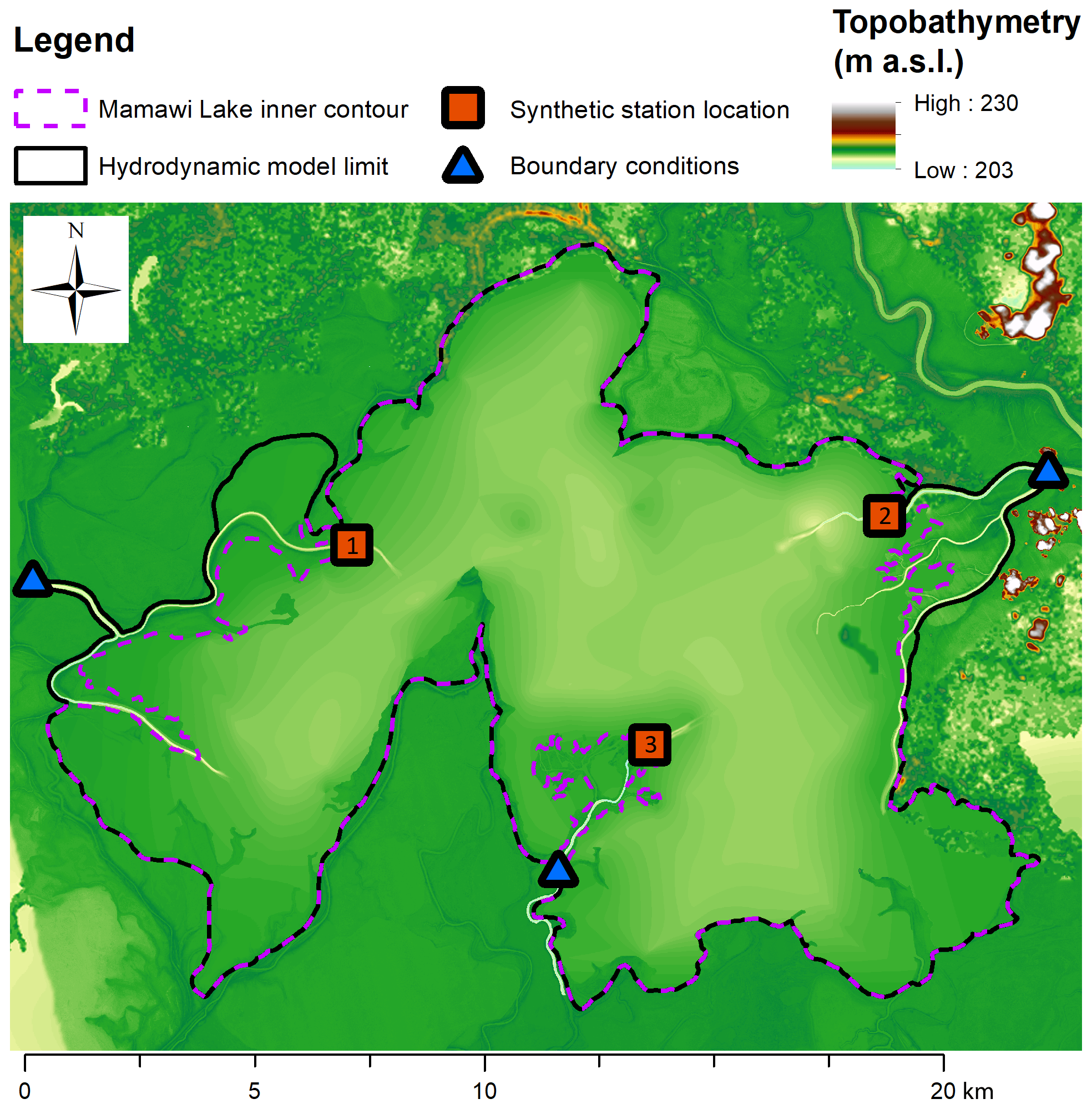
Figure 2Map of Mamawi Lake with the following elements: topobathymetry of Mamawi Lake (note that the channels are much deeper than the lake itself), Mamawi Lake water mask used to limit the extent of the hydrodynamic model (black line), inner lake contour used to compute water volumes (violet dashed line), water level observations used as boundary conditions in the hydrodynamic model (blue triangle) and synthetic hydrometric station locations for point measurements (orange squares).
A high-resolution digital elevation model (DEM; 2 m) was developed using light detection and ranging (LiDAR) elevation information provided by Environment and Climate Change Canada (ECCC) from the collection of aerial remote sensing campaigns in September 2012 and 2013. Since the LiDAR DEM covers only part of the study area, missing areas were covered by data from the Shuttle Radar Topography Mission (SRTM), downscaled to the resolution of the LiDAR DEM using bicubic interpolation. Additional details of the DEM are provided by Siles et al. (2020). All elevation data were referenced to the NAD83 Canadian spatial reference system (CSRS) and Canadian Geodetic Vertical Datum (CGVD) 2013, epoch 2010. The DEM and bathymetry were used to create the topobathymetry raster file incorporated in the hydrodynamic modelling.
The extent of Mamawi Lake is difficult to estimate precisely, both from remote sensing and in situ observations, due to the heavy vegetation and soft soil (mud) surrounding it and the seasonal variability in the water level, causing the lake to sometimes merge with neighbouring lakes to form a single water body in extreme cases. Nonetheless, a water mask that discriminated the water from the land pixels, and was used by the SWOT-HR simulator, was determined from the combination of a Sentinel-2 image acquired on 9 July 2017 and a Sentinel-1 image (Fig. 3a) acquired on 8 July 2017. This mask was also used to limit the physical boundaries of the lake in the hydrodynamic model. For the period considered in this study, the extent of the model is capped at 193 km2, including reaches, while the inner lake extent is 175 km2. The classification shown in Fig. 3b was estimated from the Sentinel-2 imagery using the image classification tool of the ArcGIS software. A supervised classification, using the maximum likelihood algorithm, was used from training polygons made from visual interpretations of photographs taken during the campaign and knowledge of the site. This classification was used to calibrate the Manning coefficients used in the hydrodynamic model (see Sect. 4).
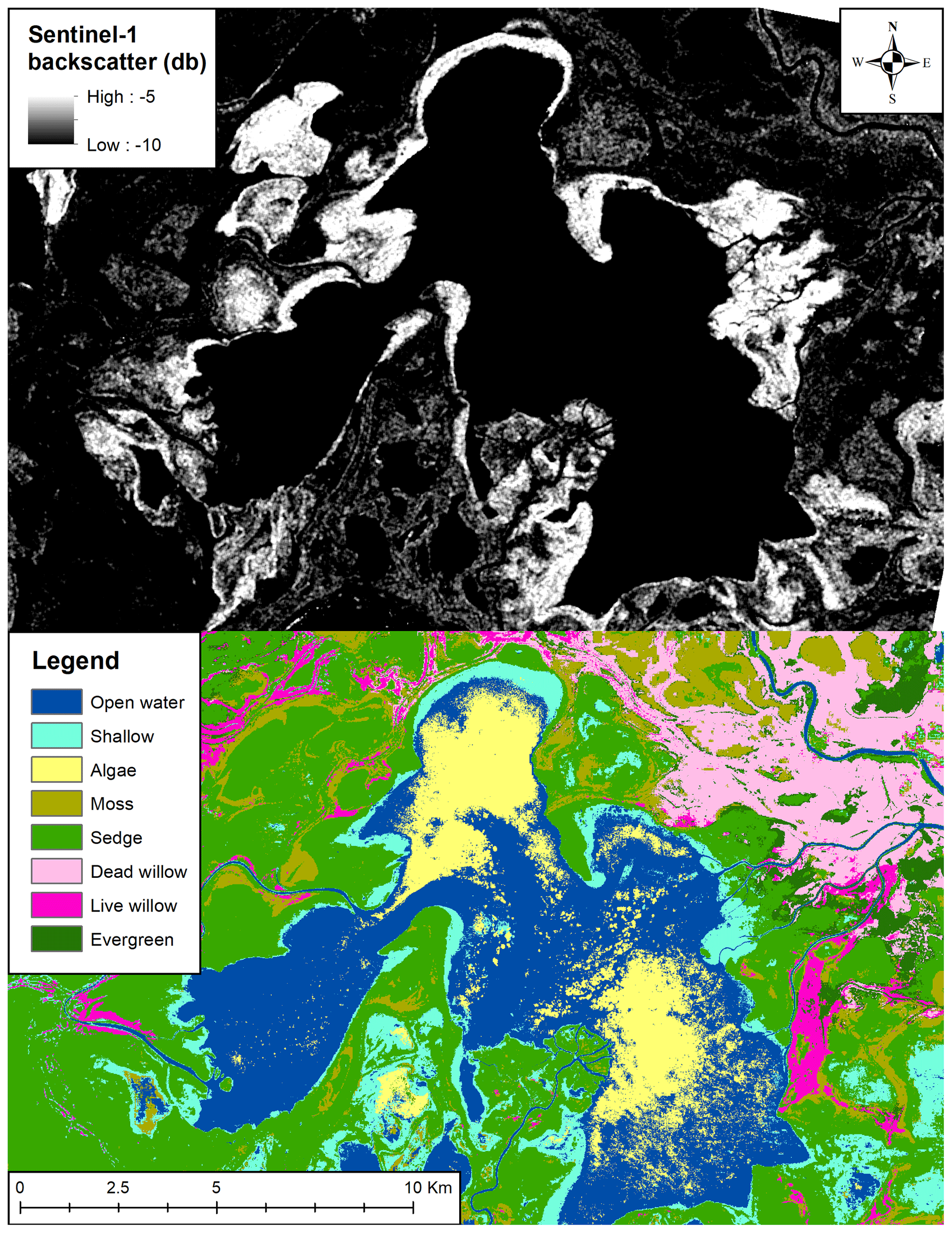
Figure 3(a) Backscattering image of Mamawi Lake taken from Sentinel-1 on 8 July 2017. (b) Supervised classification of Mamawi Lake using Sentinel-2 data taken on 9 July 2017.
4.1 Hydrodynamic simulations of Mamawi Lake
The 2D-H2D2 hydrodynamic model was used to analyze water motions beneath Mamawi Lake's surface. This finite element hydrodynamic software platform, developed at the Institut National de la Recherche Scientifique, Centre Eau Terre Environnement (INRS-ETE; Secretan, 2013), consists of multiple modules (e.g., sediment transport and water quality). H2D2 estimates the 2D flow velocities, discharge and water levels by solving the differential shallow water equations, also known as the Saint-Venant equations.
The triangular finite element mesh of the topobathymetry used in the hydrodynamic model was generated using the Surface Water Modelling System (SMS). SMS, developed by Aquaveo, was designed for 2D coastal and riverine modelling. A total of 301 900 elements were used to model Mamawi Lake. Each of these elements has an elevation, which was obtained from the topobathymetric map generated from the field measurements, and a Manning roughness coefficient.
The Manning coefficients were estimated in a two-step process. First, a supervised classification was performed using Sentinel-2 data (Fig. 3b), which was validated using pictures taken from the ground, boat and helicopter. The classes include open water, shallow or flooded areas, algae, moss, sedge, live deciduous (mainly willows), denuded or dead willows (likely caused by successive tent caterpillar outbreaks; Gleeson, 2017) and evergreen vegetation. Since the classification matched our general knowledge of the lake configuration relatively well, and the experiment is ultimately synthetic, it felt unnecessary to use a robust validation method traditionally used in remote sensing. The classification was instead used to infer starting Manning coefficient ratios for groups of classes. The classes of open water, river, shallow and algae were grouped and given the same starting values of n=0.018, a typical value for relatively smooth channels. The second step was to vary these coefficients in such a way so as to match the water level conditions measured in the channels leading to Mamawi Lake, assuming steady-state conditions. The coefficients for the other classes were also varied, while keeping the same ratio as with the former group of classes. Coefficients for areas with the moss class were compared twice with the first group, while the coefficients for remaining heavily vegetated classes (sedge, willows and evergreen) were four times those of the first group.
Once calibrated, the H2D2 simulations were assumed to represent the synthetic true state of Mamawi Lake. Several simulations were performed in transient mode over a period of 24 h under various wind conditions. Every scenario began with the steady-state result under no wind (0 m s−1) and ended after 1 d of constant wind speed and direction. The scenarios include wind speeds of 5, 10 and 15 m s−1 coming from different directions, including the cardinal and intercardinal points.
Homogenous wind speed and direction over the simulation period was a simplification of reality. However, true wind observations are not required as the results are not compared with real data. This also allowed for a simpler analysis of the simulation results and a first step towards a more thorough understanding of expected SWOT performance under more complex wind scenarios.
The H2D2 model used three boundary conditions located up (or down) the main channels leading to (or out) of the lake. Two of these were water levels, used at the Prairie River (west end) and Mamawi Channel (east end), while the third, located closer to the lake at Mamawi Creek, was set using a fixed inflow (Fig. 2). The boundary conditions were kept the same throughout the simulations. In reality, the wind could accelerate the flow downstream or slow the flow such that water accumulates upstream. However, the boundaries were specified a few kilometres outside the lake mask. This was done to reduce the impact of boundary conditions on lake water levels and avoid model divergence.
4.2 SWOT height simulations
From the four expected SWOT overpasses over Mamawi Lake, the one that covers the entire lake surface was selected (pass no. 303; Fig. 1). The SWOT-HR simulator, developed by NASA's JPL and installed at the CNES, was used to simulate expected height observations retrieved from SWOT. As input for the simulator, the H2D2-simulated water heights and the mask generated from the Sentinel-2 data, both integrated into a unique netcdf file, were used. Alternatively, the topobathymetry and a water depth file can be used as inputs. Note that, for our purposes, the high-resolution DEM was used as the truth and the reference DEM, but if other types of analyses are targeted (e.g., impact of the topographic errors in the SWOT observations) then different quality DEMs could be used. From these inputs, interferograms (IFGs) were generated that contain the phase information from which the water levels were derived.
The noise in the IFG that is later translated as the error height can be one of two types. The first type of error is a Gaussian noise that is added to the simulated Single Look Complex (SLC) images and comes from the instrument. This unbiased instrumental noise corresponds to a mean average error of 4–5 cm km−2 and can be reduced by an averaging procedure. The second type of error is of a deterministic nature and comes from the topographic layover. This error introduces a bias on the estimated heights. As explained by Oubanas et al. (2018) this noise will depend on several factors, such as the surface type and the radar parameters. The noisy phases contained in the IFG are averaged by a procedure known as multilooking to improve the signal-to-noise ratio (SNR) at the expense of resolution (e.g., Ulaby and Long, 2014). From the IFGs, pixels clouds were derived by the simulator, which were classified and geolocated. It is important to highlight that the output pixel cloud can have important geolocation errors and that the synthetic noisy SWOT phases do not include other sources of perturbation (e.g., wet and dry troposphere and ionospheric effects) that can disturb the actual signal of the satellite (Domeneghetti et al., 2018), as reported for other altimeters (e.g., Frappart et al., 2015). Among the nonsimulated errors, the residuals from the roll error that are not corrected are the ones that can have a more critical impact. At the lake scale, this error can be considered as a bias.
In order to simulate the SLC images, the simulator uses preliminary defined classes based on the values of the radar backscatter coefficient σ0. Based on previous studies (e.g., Domeneghetti et al., 2018; Moller and Esteban-Fernandez, 2015; Fjørtoft et al., 2014), σ0 values ranging from −5 to 10 dB and from 10 to 15 dB reasonably represent the signal coming from land and water, respectively. During the pixel cloud processing, the output pixel cloud is classified according to four principal classes (land, land near water, water near land and interior water), with the possibility to add a fifth class corresponding to the dark water (Peral et al., 2014) by using a specific dark water algorithm. The dark water pixels correspond to pixels that were not identified during the classification procedure because of a low local backscattering signal (e.g., calm water). An a priori Pekel mask (Pekel et al., 2016) is used in the processing to detect the possible water areas and, therefore, supports the identification of dark water patches. We emphasize that heights derived from dark water pixels are particularly noisy.
Another point to note is that the classification is impacted by the wind speed and direction. SWOT-HR uses a predefined wind field over every region in the world. The mean wind speed value extracted for the region is used to generate spatially correlated random wind fields locally. This implies that the wind speed considered by the SWOT-HR simulator differs from the wind speed specified in the hydrodynamic model and is constant across scenarios. The resulting classifications will only differ from the impact of the local WSE differences between the scenarios.
To assess the performance of the products generated by the SWOT-HR simulator, synthetic heights were compared to the simulated H2D2 elevations, which are considered as the actual observations. For this purpose and, similar to Domeneghetti et al. (2018), the SWOT-derived height pixels clouds were averaged over a window of 25 m by 25 m to estimate the error of the water levels. The mean error, and the root mean square error, were also calculated and used as global quality indicators of the heights derived from the SWOT raw data (i.e., pixel cloud).
4.3 Lake water volume analysis
In order to remain true to the goal of the study of evaluating expected SWOT performance over lakes and not rivers, which have their own set of challenges, a mask was created to exclude the channels going in and out of the lake. Henceforth, WSE and water volumes refer to the area within the mask (Fig. 2), unless stated otherwise. The water balance of Mamawi Lake was performed for two types of data, namely SWOT imagery and in situ gauges.
The first type of data is from simulated SWOT imagery. WSE over the entire lake was retrieved in two ways. The first is computed using the mean elevation of SWOT pixels, assuming the WSE to be uniform over the lake. The second is computed by passing a linear plane through available SWOT pixel cloud data, such that the square of the normal distance between the plane and the pixel cloud is minimized. This was performed for different hypothetical passes covering various areas of the lake in order to assess the impact of the spatial coverage on the water volume retrieval. Though the lake size (approximately 19 km at its widest orbital-wise) is smaller than the swath width (50 km), fractional coverage of the lake could be obtained if the lake was located close to the nadir or far range. These potential coverage scenarios are represented in Fig. 4, where each colour represents a coverage band in increments of 10 %.

Figure 4Hypothetical spatial coverage scenarios based on the expected SWOT pass no. 303 over Mamawi Lake.
WSE difference, or water volume between two hypothetical passes, could be extracted and compared with the true values extracted from the H2D2 model. Since every wind scenario lasted 24 h, the result of which is used as input in the simulator, it was assumed that the time between SWOT passes also corresponded to 24 h. When a fractional coverage of the lake was specified, for example 20 %, it was assumed that only 20 % of the lake was covered for the first pass at the beginning of the simulation when wind speed is 0 m s−1 and 20 % for the second pass after 24 h of constant wind. Every combination of 20 % coverage cases was considered when retrieving water volumes. These are broken down in the following way: east and west coverage for time = 0 h and time = 24 h, adding up to a total of four cases per coverage band. Different water volumes can be retrieved from these four samples and converted into average net flow by dividing the volume by the time interval between the two hypothetical passes.
The water volumes were also compared with volumes estimated, using synthetic pressure gauges spread over the lake for benchmarking purposes. It was assumed that the gauges would normally be located in easily accessible sites. Therefore, three gauges were added near the main channels around the lake (Fig. 2).
WSE from gauges were computed in two different ways. The simplest way consists of applying the synthetic gauge reading, or the average readings for multiple gauges, over the entire lake, assuming a uniform elevation throughout. The second approach uses linear planes computed differently, depending on the number of available gauges. For one available gauge, it was assumed that the lake had a uniform elevation of equal value to the one extracted from gauge no. 1 (see Fig. 2). This synthetic gauge is closest to an existing hydrometric network gauge of the Water Survey of Canada in the channel connecting the west side of Mamawi Lake with Lake Claire. If two gauges were assumed to be available, a second gauge was added at the largest branch of Mamawi Channel to the east. A linear plane was created, using a vector connecting these two elevations and a second vector perpendicular to the former vector. This plane was used to extrapolate over every point in the lake. Finally, when three gauges were assumed to be available, the gauge near the delta formed by Mamawi Creek to the south was also considered. A linear plane could be traced through each point and extrapolated throughout the rest of the lake. As with SWOT data, the water volume between passes was compared with the true values extracted from the H2D2 model.
Each gauge was assumed to have an unbiased normally distributed error of 0.5 cm centered around the true WSE value extracted from the hydrodynamic model. To take the gauge error into consideration, 100 samples were taken for each time step, creating as many pairs of linear planes for WSE.
5.1 Hydrodynamic simulations of the Mamawi Lake
A total of 25 simulations were performed using the H2D2 model. The first one is the scenario without wind (0 m s−1), which is the starting point for all the other simulations. The remaining 24 wind scenarios include all eight directions (cardinal and intercardinal points) applied to all the other wind speeds (5, 10 and 15 m s−1). Examples are shown in Fig. 5.
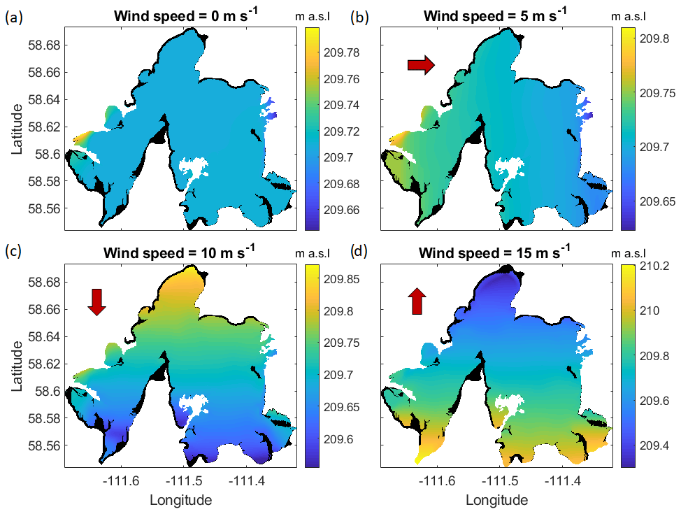
Figure 5A sample of the water surface elevation (WSE) results from the H2D2 simulations. (a) No wind; (b) 5 m s−1 wind coming from the east; (c) 10 m s−1 wind coming from the south; (d) 15 m s−1 wind coming from the north. Black areas represent no water. Note that the scale differs between figures for visibility purposes. The red arrows point in the direction of the incoming wind.
The constant wind over 24 h was sufficient to cause the water levels to adjust in a gradient following the direction of the outgoing wind. The gradient becomes stronger as wind speed increases. Some exceptions can be noticed near the eastern and western channels, resulting from the water flowing over the banks from or into the nearby channels, which are omitted by the lake mask, via a more direct way than the main route. These areas are also strongly vegetated, with relatively high Manning coefficients, allowing for steeper slopes to form than on the open water lake area. Though the lake mask aimed to reduce this effect, it was not adjusted to exclude those regions. It is unknown whether or not this reflects the real behaviour of the lake, but it is nonetheless the true state as simulated by H2D2. It also allows for some local heterogeneities, which can be found in real lakes from nearby channels. for example, without being dominated by this effect.
5.2 SWOT height simulations
A total of 25 synthetic WSE maps for Mamawi Lake were generated using the SWOT-HR. An example of the classification for two different scenarios corresponding to a wind of 0 and 15 m s−1 blowing from the north is presented in Fig. 6a and b, respectively. As observed, the classification of pixels is similar in both scenarios, except for some areas (highlighted in red) where more significant differences are noticed. The similarities come from the constant wind field maps used by the SWOT-HR simulator. For all the simulated scenarios, most pixels belong to the interior water class and a small number to the water near land edge class. The SWOT-derived WSE are centered around a mean value of 209.77 ± 0.37 m for all scenarios when considering only wet pixels (classes 3 and 4). It must be taken into account that, when including the dark water class, the signal corresponds mainly to noise and, therefore, the quality of the retrieved geolocated heights for these pixels can be notably deteriorated.
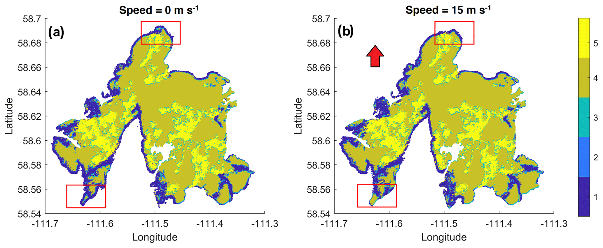
Figure 6Classification examples corresponding to two different wind scenarios. The legend is as follows: 1 – land; 2 – land near water; 3 – water near land edge; 4 – interior water; 5 – dark water. The red arrow points in the direction of the incoming wind.
Some examples of the retrieved SWOT pixel cloud heights are shown in Fig. 7. They correspond to the same scenarios as in Fig. 5. Despite the water extent being similar across the scenarios, a notable spatial variation is observed for retrieved WSE. Note also that only the pixels corresponding to the water near land edge and the interior water classes are depicted. Larger empty areas inside the lake correspond principally to dark water. Detection of these areas at low incident angles is challenging due to the low land–water contrast (Solander et al., 2016). Some of these pixels might correspond to dense areas of emergent vegetation or where the presence of algal beds is important (see Fig. 6), yet the procedures in the simulations are statistical and, therefore, mainly associated with dark water and do not reflect the actual physical reality. Similarly, some pixels inside the lake may be incorrectly classified as dry pixels (classes 1 and 2). Nevertheless, most of those pixels are generally located at the shores of the lake and are therefore expected to correspond to dry areas. From a visual inspection, the distribution of the SWOT-derived WSE is similar to those simulated by the H2D2 model and is particularly more visible for the speeds 10 and 15 m s−1. Overall, the largest over- and underestimation of WSE occurred in scenarios corresponding to speeds >5 m s−1 and to winds blowing in southerly and northerly directions.
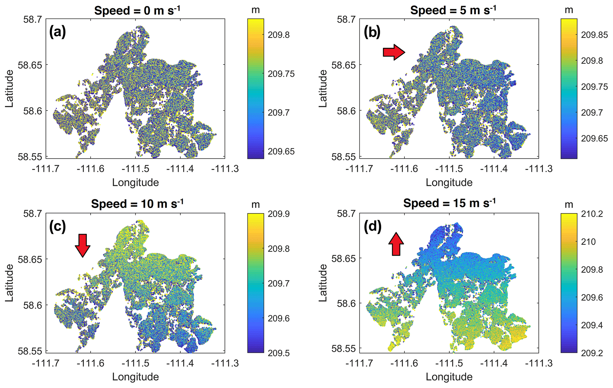
Figure 7A sample of the WSE results from the SWOT-HR simulator. (a) No wind; (b) 5 m s−1 wind coming from the east; (c) 10 m s−1 wind coming from the south; (d) 15 m s−1 wind coming from the north. The red arrows point in the direction of the incoming wind.
Figure 8 shows the mean errors (ME) and the root mean square error (RMSE) for the derived water heights for the 25 simulated scenarios. Figure 8a and b depict the ME and RMSE for the surface elevations only corresponding to wet areas (classes of interior water and water near land), respectively. Dark water pixels might be used for the estimation of water extent but not for analysis that involves the simulated heights of these pixels because, as previously stated, they are very noisy. The ME and RMSE values vary between ∼ 0.05 and m and between ∼ 0.3 and 0.7 m, respectively. If the dry and the dark water areas are considered, the ME (>0.6 m) and the RMSE (>2 m) notably increased (Fig. 8c and d). This result is not surprising since the KaRIn band height retrieval algorithm is not expected to perform well on areas corresponding to land and/or darker surfaces (Solander et al., 2016; Domeneghetti et al., 2018). Some pixels affected by layover and other geometrical effects may also introduce important outliers, particularly those located near land, although they could be within the lake (interior water class).
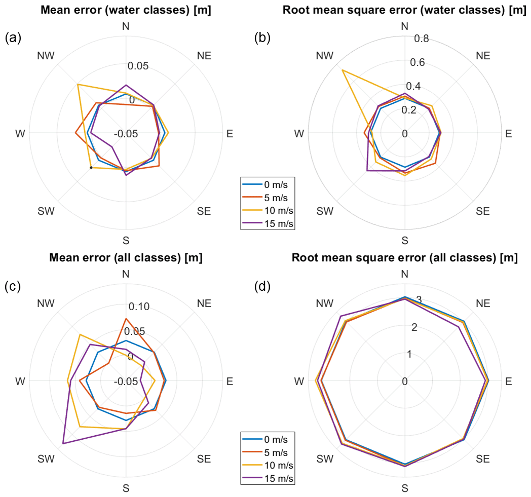
Figure 8(a) Mean and (b) root mean square errors (RSMEs) on WSE as a function of incoming wind direction using wet pixels only. Similarly, (c) and (d) correspond to the mean error and RMSE, including all pixel classes within the lake mask.
The largest outliers in Fig. 8a correspond to the scenario in which wind coming from the northwest at a speed of 10 m s−1 is simulated. The larger errors (ME – 0.05 m; RMSE – 0.7 m) for this scenario might be more important because of the orientation of the wind and the water movement with respect to the satellite track which is descending, but this is principally from a misclassification of pixels. The direction of the water movement may create a slope (adding to the natural slope of the lake; Fig. 5a) for which disposition, with respect to the satellite-viewing geometry, might have the same effect as an embankment of a river in the near range. This disposition can produce layover and other geometrical distortions that may be more significant when considering all the pixels classes. Points affected by these types of distortions are possibly affected by larger geolocation errors (e.g., Domeneghetti et al., 2018). Moreover, the source of large outliers can also come from the averaging of pixels and from the interpolation from resampling the pixel cloud into the grid of the elevations derived from the hydrodynamic model. Indeed, by inspecting the error maps, some of the larger errors are found at locations where the interpolation is applied to fill gaps. Therefore, these errors might not correspond to the actual errors associated to the SWOT products, and direct comparison with the mission requirements may be not be reasonable, as suggested by Domeneghetti et al. (2018). Other important mean errors are also identified in other incoming wind directions in Fig. 8a and b. For example, a high RMSE is noted (>0.4 m) for the case of wind blowing at 15 m s−1 and coming from the southwestern direction.
Another issue to address is the mismatch between the wind fields used in the hydrodynamic model and the SWOT-HR simulator. Although not directly a source of error on retrieved WSE, it likely misrepresents the classification expected from a real experiment. Using the 0 m s−1 wind speed scenario as an example, most of the lake would likely be mostly covered by dark water pixels in reality, except for areas with vegetation. Using SWOT-HR, most of the lake was classified as interior water, which is technically correct but is an optimistic expectation from a real result. On the other end of the spectrum, scenarios with a high constant wind speed are unlikely to have as many dark water pixels as provided by SWOT-HR. Although the mismatching wind fields only directly affect the classification, it also indirectly affects the number of SWOT pixels available for retrieving WSE since only some pixel classes are considered to determine the WSE. Depending on the wind scenario specified in the hydrodynamic model, there may be more or fewer pixels available for WSE retrievals than what is considered in this study. The ability to modify wind fields within the simulator to reflect those used in the hydrodynamic model would provide greater coherence within the scenarios.
5.3 Lake water volume and net flow analysis
The difference between net flows retrieved from the synthetic gauges and true net flows are shown in Figs. 9a and 10a for the uniform and linear plane approaches to extrapolate WSE, respectively. The results are aggregated according to the number of available stations. Each box summarizes 100 samples to take the gauge error into consideration. As a reference, the true average net flow for 5, 10 and 15 m s−1 wind scenarios are −0.09, −4.45 and −10.88 m3 s−1, respectively, corresponding to a net flow out of the lake. The inflow averages between 130 and 154 m3 s−1, to put the numbers into perspective.

Figure 9Net flow difference between flows retrieved from the true state and either (a) synthetic gauge measurements, as a function of available station, or (b) SWOT pixel cloud, as a function of lake area covered, assuming a uniform WSE. Every scenario begins with a windless case and ends after 24 h of constant wind. All wind scenarios are merged into a single box.
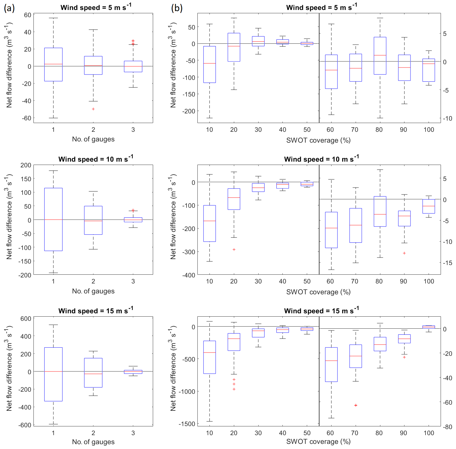
Figure 10Net flow difference between flows retrieved from the true state and either (a) synthetic gauge measurements, as a function of available station, or (b) SWOT pixel cloud, as a function of lake area covered, assuming the WSE follows a linear plane. Every scenario begins with a windless case and ends after 24 h of constant wind. All wind scenarios are merged into a single box. It should be noted that the scales differ between (a) and (b), and that the (b) plots are split using separate scales for lower (0 %–50 %) or higher (>50 %) coverage for visibility purposes.
As expected, net flow difference decreases as the number of gauges, or the amount of information available, increases. This is the case for all wind speeds. Conversely, net flow difference increases as wind speed increases. Since the gauges are stationed relatively close to the center of the lake, they are less susceptible to the change in water level caused by the wind. The effect of local heterogeneities shown in Fig. 5 also has little effect on the results since they occur away from the gauges. It should also be noted that, when multiple gauges are available, using a linear plane to extrapolate WSE yields more accurate retrievals at higher wind speeds, which is when the lake WSE becomes less uniform.
The patterns observed with synthetic gauges are also present in the flow difference analysis for SWOT retrievals (Figs. 9b and 10b for uniform and linear plane approaches to extrapolate WSE, respectively). The results are aggregated according to the percentage of lake area covered by SWOT passes. Each box summarizes the combinations of wind directions and lake side covered, namely two sides (east or west end) for the first pass and eight wind directions for each of the two sides of the lake that is covered for the second pass. This makes a total of scenarios for each percent band of lake coverage.
In general, as wind speed increases, so does the error in net flow retrievals. As lake coverage increases, more information is added, and the flow error decreases. This is the case for all wind speeds but is amplified when compared with gauges. This is partly the result of the noise parameters specified in the SWOT-HR simulator but is also amplified by the local heterogeneities seen in Fig. 5. Since these heterogeneities occur at the eastern and western ends of the lake, which are covered in the first or last 10 % band, they have a large impact on water level interpolation, particularly for low lake coverage (see Fig. 4 for SWOT pass coverage) and particularly if a linear plane is used to extrapolate WSE. For example, WSE retrieved from a first pass covering only the first 10 % of the eastern end of the lake might be lower than the rest of the lake. As a result, WSE generated assuming a uniform level would be underestimated. On the other hand, the linear plane might increase drastically toward the western end due to the local slope, resulting in an increasingly underestimated retrieval as the local slope increases. If the following pass after 24 h only covers the first 10 % of the opposite (western) end, the WSE estimated from the uniform approach would be overestimated, while the linear plane would decrease drastically toward the eastern end, resulting in an underestimation of WSE. The resulting net flow would be positive, with a uniform water level approach, and negative, using a linear-plane approach. Over- and underestimations are both present in the figures. As more lake area is covered, the effect of these heterogeneities decreases. Similarly, this effect reduces as wind speed increases as the changes in lake WSE becomes more important. However, unlike synthetic gauges, there is a flow retrieval bias for low area coverage, particularly for the linear-plane approach. This is mainly caused by the asymmetric effect of wind on lake water levels. This is demonstrated in Fig. 11 for the retrieval of lake water volume at wind speeds of 15 m s−1 and 10 % lake coverage, using the linear-plane approach as an example. The error for a given pass is not entirely symmetrical around the cardinal and intermediate directions. The largest differences in retrieved water volume generally occur when the incoming wind is in an east–west axis, which is the same as the general flow in the lake, and the partial coverage is in the opposite direction of the incoming wind. The average error for all passes combined is lowest when the wind is coming from the north, followed by the south, both of which are perpendicular to the natural flow. The effect of the wind on retrievals is not entirely symmetrical between passes, resulting in a bias seen in Fig. 10b.
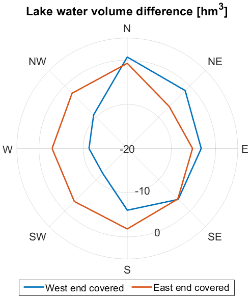
Figure 11Lake water volume difference between the true state and the volume retrieved from the SWOT pixel cloud, using a linear plane to extrapolate WSE as a function of incoming wind direction for a constant wind speed of 15 m s−1 over 24 h. A lake coverage of 10 % is used. The blue curve represents a pass where only the west end of Mamawi Lake is covered, while the red curve represents a coverage of the eastern end.
When the SWOT coverage is low, retrievals from even a single synthetic point measurement are more reliable. However, as SWOT coverage increases, the retrievals become increasingly precise, to the point where a 100 % lake coverage yields more reliable results than the three synthetic gauges combined.
The study, one of several ongoing SWOT-C TH (Pietroniro et al., 2019), compared water heights computed by the SWOT-HR hydrology simulator with those provided by the H2D2 hydrodynamic model under various wind scenarios. Resulting estimates of water storage were also compared with those provided by gauge measurements within a synthetic framework. The analysis of the results highlighted the importance of having a high percentage of lake coverage included in SWOT passes, particularly in the presence of local heterogeneities. The accuracy of retrievals was also shown to depend on the method used to extrapolate WSE. An approach assuming uniform water levels was shown to be less prone to large errors, particularly for low lake coverage, compared with an approach using a linear plane, which seems to produce better results for a lake with 100 % coverage. This is one of the methods included in the LOCNES toolbox developed by the CNES, which can be used to produce lakes products, such as WSE, extent and water storage (e.g, Pottier and Cazals, 2019).
The results presented are conditional to a number of assumptions and limitations. To begin, the study rests on the synthetic framework generated by hydrodynamic model and a number of parameters driving it. The physically based nature of the model is assumed to reflect the general behaviour of a real scenario under similar circumstances. This excludes the possibility of underground channel formations, water seeping out of the modelled lake aside from specified boundaries. It also does not consider evapotranspiration, which should be negligible compared with channel inflow and outflow over a period of 24 h. Small waves normally generated under the influence of wind were not explicitly simulated at the scale used by the model, and their presence may influence SWOT height retrievals.
A similar argument can be applied to the SWOT-HR simulator, which was designed to represent expected images from a real instrument, including noises from various sources. However, known potential issues might need to be further analysed, such as dark water surfaces which can mislead the classification (e.g., Solander et al., 2016). Errors related to the geolocation due to geometrical distortions, DEM errors and other factors, such as flooded vegetation, need to be considered in the accuracy assessment. One possible solution to mitigate these types of errors would be through a postprocessing of the pixel cloud by using the LOCNES. Additionally, the Radarsat Constellation Mission (RCM), which provide a higher frequency of observations, could also help to improve the water balance estimation by providing external complementary information (e.g., over flooded vegetation). Nevertheless, the use of a single SWOT pass with identical orbital parameters for every simulation also limits the generalizations of the conclusions.
There is also the issue of the mismatch between the wind field used in the hydrodynamic model and the classification made by the SWOT-HR simulator. The results provided in this study may underestimate or overestimate the real error from SWOT retrievals, depending on the representativity of the classification. The inability to specify wind fields in the SWOT-HR simulator currently limits the transferability of the results to real scenarios.
Another assumption pertains to the WSE results obtained which are specific to Mamawi Lake, including its size, shape and location of boundary conditions. It is expected that similar results would be obtained from lakes sharing similar characteristics. Applying the conclusions of this study to lakes and reservoirs of different shapes and sizes could be considered if changes in WSE within the lake remain in good approximation to a plane. This is particularly important if only a small portion of the lake is covered by the SWOT image.
Finally, simulations under constant wind speeds and directions were performed in this study. This restriction resulted in lake water levels that are relatively well approximated by a linear plane. If wind conditions were not constant in strength or direction, there may be stronger local heterogeneities in lake water levels that could lead to greater errors for partial SWOT coverage, just as it could for pressure gauges.
These assumptions and limitations represent challenges that may be used to stimulate future studies. These could include the introduction of nonuniform wind conditions, the use of longer or shorter periods between SWOT passes, using multiple SWOT passes with varying spatial coverages and orbital parameters, such as varying incidence angle, evaluating the effect of flooded vegetation or aquatic vegetation on SWOT retrievals, using more complex interpolation and extrapolation methods to retrieve lake water levels, and allowing validation over a wider range of lake sizes and geometries.
Continued scientific progress is encouraged as the SWOT mission has the potential to provide an unprecedented ability to monitor spatially distributed channel, lake and wetland WSE such as the Peace–Athabasca delta complex, where the Wood Buffalo National Park Action Plan was developed in response to a UNESCO Reactive Mission Report that assessed potential threats to the delta ecosystem. A novel satellite-based surface water monitoring approach would enhance the ability to address environmental flows–hydrology components that traditionally relied on sparse ground-based monitoring.
Sentinel-1 and Sentinel-2 imagery can be obtained freely from the Copernicus open access hub, SciHub (https://scihub.copernicus.eu/, Copernicus, 2020). At the time of publishing, the SWOT-HR simulator is not accessible to the public.
RL, DLP and MT acquired the funding. JB and RL designed the overall methodology, with assistance from GS for the steps specific to the SWOT-HR simulations. JB began the investigation by carrying out the hydrodynamic simulations and its formal analysis, assisted by RL and MT. GS carried out the SWOT-HR simulations, assisted by DD, and its formal analysis. JB, RL, DLP, GS and MT all contributed to the fieldwork campaigns over the Peace–Athabasca delta. JB and GS prepared the paper, with contributions from all other coauthors.
The authors declare that they have no conflict of interest.
We thank Environment and Climate Change Canada and Parks Canada for their collaboration in this study. In particular, we thank David Campbell, Ronnie Campbell, Tom Carter, Mark Russell, Sébastien Langlois, Jessica Lankshear and Nicolas Simard for helping to collect data during the 2017 field campaign. We are also thankful for the tips given by Pascal Matte and Sébastien Langlois for setting up the H2D2 model and improving its efficiency. We thank the CNES for providing access to the SWOT-HR simulator and processing tools, which were all developed by the SWOT JPL project.
This research has been supported by the Canadian Space Agency (grant no. 14SUSWOTSH).
This paper was edited by Micha Werner and reviewed by Guy J.-P. Schumann and one anonymous referee.
Baup, F., Frappart, F., and Maubant, J.: Combining high-resolution satellite images and altimetry to estimate the volume of small lakes, Hydrol. Earth Syst. Sci., 18, 2007–2020, https://doi.org/10.5194/hess-18-2007-2014, 2014.
Beltaos, S.: Comparing the impacts of regulation and climate on ice-jam flooding of the Peace-Athabasca Delta, Cold Reg. Sci. Technol., 108, 49–58, https://doi.org/10.1016/j.coldregions.2014.08.006, 2014.
Biancamaria, S., Lettenmaier, D. P., and Pavelsky, T. M.: The SWOT Mission and Its Capabilities for Land Hydrology, Surv. Geophys., 37, 307–337, https://doi.org/10.1007/s10712-015-9346-y, 2016.
Bioresita, F., Puissant, A., Stumpf, A., and Malet, J.-P.: Fusion of Sentinel-1 and Sentinel-2 image time series for permanent and temporary surface water mapping, Int. J. Remote Sens., 40, 1–24, https://doi.org/10.1080/01431161.2019.1624869, 2019.
Bonsal, B. R., Peters, D. L., Seglenieks, F., Rivera, A., and Berg, A.: Changes in freshwater availability across Canada, in: Canada's changing climate report, edited by: Bush, E. and Lemmen, D. S., Government of Canada, Ottawa, Ontario, Canada, 261–342, 2019.
Brenner, A. C., DiMarzio, J. P., and Zwally, H. J.: Precision and accuracy of satellite radar and laser altimeter data over the continental ice sheets, IEEE Trans. Geosci. Remote Sens., 45, 321–331, https://doi.org/10.1109/TGRS.2006.887172, 2007.
Bush, A., Monk, W. A., Compson, Z. G., Peters, D. L., Porter, T. M., Shokralla, S., Wright, M. T. G., Hajibabaei, M., and Baird, D. J.: DNA metabarcoding reveals metacommunity dynamics in a threatened boreal wetland wilderness, Proc. Natl. Acad. Sci., 117, 201918741, https://doi.org/10.1073/pnas.1918741117, 2020.
Bwangoy, J. R. B., Hansen, M. C., Roy, D. P., Grandi, G. D., and Justice, C. O.: Wetland mapping in the Congo Basin using optical and radar remotely sensed data and derived topographical indices, Remote Sens. Environ., 114, 73–86, https://doi.org/10.1016/j.rse.2009.08.004, 2010.
Copernicus: Sentinel data 2017, available at: https://scihub.copernicus.eu/, last access: 7 December 2020.
Crétaux, J. F. and Birkett, C.: Lake studies from satellite radar altimetry, Comptes Rendus-Geosci., 338, 1098–1112, https://doi.org/10.1016/j.crte.2006.08.002, 2006.
Crétaux, J. F., Abarca-del-Río, R., Bergé-Nguyen, M., Arsen, A., Drolon, V., Clos, G., and Maisongrande, P.: Lake Volume Monitoring from Space, Surv. Geophys., 37, 269–305, https://doi.org/10.1007/s10712-016-9362-6, 2016.
da Silva, J. S., Calmant, S., Seyler, F., Moreira, D. M., Oliveira, D., and Monteiro, A.: Radar altimetry aids managing gauge networks, Water Resour. Manag., 28, 587–603, https://doi.org/10.1007/s11269-013-0484-z, 2014.
Ding, X. W. and Li, X. F.: Monitoring of the water-area variations of Lake Dongting in China with ENVISAT ASAR images, Int. J. Appl. Earth Obs. Geoinf., 13, 894–901, https://doi.org/10.1016/j.jag.2011.06.009, 2011.
Domeneghetti, A., Schumann, G. J. P., Frasson, R. P. M., Wei, R., Pavelsky, T. M., Castellarin, A., Brath, A., and Durand, M. T.: Characterizing water surface elevation under different flow conditions for the upcoming SWOT mission, J. Hydrol., 561, 848–861, https://doi.org/10.1016/j.jhydrol.2018.04.046, 2018.
Duan, Z. and Bastiaanssen, W. G. M.: Estimating water volume variations in lakes and reservoirs from four operational satellite altimetry databases and satellite imagery data, Remote Sens. Environ., 134, 403–416, https://doi.org/10.1016/j.rse.2013.03.010, 2013.
Farhadzadeh, A., Hashemi, M. R., and Neill, S.: Characterizing the Great Lakes hydrokinetic renewable energy resource: Lake Erie wave, surge and seiche characteristics, Energy, 128, 661–675, https://doi.org/10.1016/j.energy.2017.04.064, 2017.
Fjørtoft, R., Gaudin, J. M., Pourthié, N., Lalaurie, J. C., Mallet, A., Nouvel, J. F., Martinot-Lagarde, J., Oriot, H., Borderies, P., Ruiz, C., and Daniel, S.: KaRIn on SWOT: Characteristics of near-nadir Ka-band interferometric SAR imagery, IEEE Trans. Geosci. Remote Sens., 52, 2172–2185, https://doi.org/10.1109/TGRS.2013.2258402, 2014.
Frappart, F., Fatras, C., Mougin, E., Marieu, V., Diepkilé, A. T., Blarel, F., and Borderies, P.: Radar altimetry backscattering signatures at Ka, Ku, C, and S bands over West Africa, Phys. Chem. Earth, 83/84, 96–110, https://doi.org/10.1016/j.pce.2015.05.001, 2015.
Frasson, R. P. D. M., Wei, R., Durand, M., Minear, J. T., Domeneghetti, A., Schumann, G., Williams, B. A., Rodriguez, E., Picamilh, C., Lion, C., Pavelsky, T., and Garambois, P.-A.: Automated River Reach Definition Strategies: Applications for the Surface Water and Ocean Topography Mission, Water Resour. Res., 53, 8164–8186, https://doi.org/10.1002/2017WR020887, 2017.
Garambois, P. A. and Monnier, J.: Inference of effective river properties from remotely sensed observations of water surface, Adv. Water Resour., 79, 103–120, https://doi.org/10.1016/j.advwatres.2015.02.007, 2015.
Gardelle, J., Hiernaux, P., Kergoat, L., and Grippa, M.: Less rain, more water in ponds: a remote sensing study of the dynamics of surface waters from 1950 to present in pastoral Sahel (Gourma region, Mali), Hydrol. Earth Syst. Sci., 14, 309–324, https://doi.org/10.5194/hess-14-309-2010, 2010.
Gleason, C. J. and Hamdan, A. N.: Crossing the (watershed) divide: satellite data and the changing politics of international river basins, Geogr. J., 183, 2–15, https://doi.org/10.1111/geoj.12155, 2017.
Gleason, C. J., Smith, L. C., and Lee, J.: Retrieval of river discharge solely from satellite imagery and at-many-stations hydraulic geometry: Sensitivity to river form and optimization parameters, Water Resour. Res., 50, 9604–9619, https://doi.org/10.1002/2014WR016109, 2014.
Gleeson, R.: Caterpillars invade Great Slave Lake area, CBC News, available at: https://www.cbc.ca/news/canada/north/caterpillars-invade-great-slave-lake-1.4161384 (last access: 16 December 2020), 2017.
Grippa, M., Rouzies, C., Biancamaria, S., Blumstein, D., Cretaux, J. F., Gal, L., Robert, E., Gosset, M., and Kergoat, L.: Potential of SWOT for Monitoring Water Volumes in Sahelian Ponds and Lakes, IEEE J. Sel. Top. Appl. Earth Obs. Remote Sens., 12, 2541–2549, https://doi.org/10.1109/JSTARS.2019.2901434, 2019.
Häfliger, V., Martin, E., Boone, A., Ricci, S., and Biancamaria, S.: Assimilation of Synthetic SWOT River Depths in a Regional Hydrometeorological Model, Water, 11, 78, https://doi.org/10.3390/w11010078, 2019.
Jiang, H., Feng, M., Zhu, Y., Lu, N., Huang, J., and Xiao, T.: An Automated Method for Extracting Rivers and Lakes from Landsat Imagery, Remote Sens., 6, 5067–5089, https://doi.org/10.3390/rs6065067, 2014.
Kim, J. W., Lu, Z., Lee, H., Shum, C. K., Swarzenski, C. M., Doyle, T. W., and Baek, S. H.: Integrated analysis of PALSAR/Radarsat-1 InSAR and ENVISAT altimeter data for mapping of absolute water level changes in Louisiana wetlands, Remote Sens. Environ., 113, 2356–2365, https://doi.org/10.1016/j.rse.2009.06.014, 2009.
Leconte, R., Pietroniro, A., Peters, D. L., and Prowse, T. D.: Effects of flow regulation on hydrologic patterns of a large, inland delta, Regul. Rivers Res. Manag., 17, 51–65, https://doi.org/10.1002/1099-1646(200101/02)17:1<51::AID-RRR588>3.0.CO;2-V, 2001.
Maheu, C., Cazenave, A., and Mechoso, C. R.: Water level fluctuations in the Plata Basin (South America) from Topex/Poseidon Satellite Altimetry, Geophys. Res. Lett., 30, 1143, https://doi.org/10.1029/2002GL016033, 2003.
Mohammadimanesh, F., Salehi, B., Mahdianpari, M., Brisco, B., and Motagh, M.: Wetland Water Level Monitoring Using Interferometric Synthetic Aperture Radar (InSAR): A Review, Can. J. Remote Sens., 44, 247–262, https://doi.org/10.1080/07038992.2018.1477680, 2018.
Moller, D. and Esteban-Fernandez, D.: Near-Nadir Ka-band Field Observations of Freshwater Bodies, in: Remote Sensing of the Terrestrial Water Cycle, edited by: Lakshmi, V., Alsdorf, D., Anderson, M., Biancamaria, S., Cosh, M., Entin, J., Huffman, G., Kustas, W., van Oevelen, P., Painter, T., Parajka, J., Rodell, M., and Rüdiger, C., American Geophysical Union (AGU), Washington, DC, USA, https://doi.org/10.1002/9781118872086.ch9, 2014.
Munier, S., Polebistki, A., Brown, C., Belaud, G., and Lettenmaier, D. P.: SWOT data assimilation for operational reservoir management on the upper Niger River Basin, Water Resour. Res., 51, 554–575, https://doi.org/10.1002/2014WR016157, 2015.
Musa, Z. N., Popescu, I., and Mynett, A.: A review of applications of satellite SAR, optical, altimetry and DEM data for surface water modelling, mapping and parameter estimation, Hydrol. Earth Syst. Sci., 19, 3755–3769, https://doi.org/10.5194/hess-19-3755-2015, 2015.
Oubanas, H., Gejadze, I., Malaterre, P.-O., Durand, M., Wei, R., Frasson, R. P. M., and Domeneghetti, A.: Discharge Estimation in Ungauged Basins Through Variational Data Assimilation: The Potential of the SWOT Mission, Water Resour. Res., 54, 2405–2423, https://doi.org/10.1002/2017WR021735, 2018.
Palmer, S. C. J., Kutser, T., and Hunter, P. D.: Remote sensing of inland waters: Challenges, progress and future directions, Remote Sens. Environ., 157, 1–8, https://doi.org/10.1016/j.rse.2014.09.021, 2015.
Pavelsky, T. M., Durand, M. T., Andreadis, K. M., Beighley, R. E., Paiva, R. C. D., Allen, G. H., and Miller, Z. F.: Assessing the potential global extent of SWOT river discharge observations, J. Hydrol., 519, 1516–1525, https://doi.org/10.1016/j.jhydrol.2014.08.044, 2014.
Pekel, J. F., Cottam, A., Gorelick, N., and Belward, A. S.: High-resolution mapping of global surface water and its long-term changes, Nature, 540, 418–422, https://doi.org/10.1038/nature20584, 2016.
Peral, E., Rodriguez, E., Moller, D., McAdams, M., Johnson, M., Andreadis, K., Arumugam, D., and Williams, B.: SWOT L1b Hydrology Simulator User Guide, Version 2, Jet Propulsion Laboratory, Pasadena, California, USA, 32 pp., 2014.
Peters, D. L. and Buttle, J. M.: The effects of flow regulation and climatic variability on obstructed drainage and reverse flow contribution in a Northern river-lake-Delta complex, Mackenzie basin headwaters, River Res. Appl., 26, 1065–1089, https://doi.org/10.1002/rra.1314, 2010.
Peters, D. L., Prowse, T. D., Marsh, P., Lafleur, P. M., and Buttle, J. M.: Persistence of water within perched basins of the Peace-Athabasca Delta, Northern Canada, Wetl. Ecol. Manag., 14, 221–243, https://doi.org/10.1007/s11273-005-1114-1, 2006a.
Peters, D. L., Prowse, T. D., Pietroniro, A., and Leconte, R.: Flood hydrology of the Peace-Athabasca Delta, northern Canada, Hydrol. Process., 20, 4073–4096, https://doi.org/10.1002/hyp.6420, 2006b.
Phillips, D.: The Climates of Canada, Ottawa, Ontario, Canada, Government of Canada Publications, 181 pp., ISBN 978-0-660-20296-9, 1990.
Pietroniro, A., Peters, D. L., Yang, D., Fiset, J.-M., Saint-Jean, R., Fortin, V., Leconte, R., Bergeron, J., Llanet Siles, G., Trudel, M., Garnaud, C., Matte, P., Smith, L. C., Gleason, C. J., and Pavelsky, T. M.: Canada's Contributions to the SWOT Mission – Terrestrial Hydrology(SWOT-C TH), Can. J. Remote Sens., 45, 116–138, https://doi.org/10.1080/07038992.2019.1581056, 2019.
Pottier, C. and Cazals, C.: Prior Lake Database, SWOT Science Team Meeting 2019, Bordeaux, France, available at: https://www.aviso.altimetry.fr/fileadmin/documents/user_corner/SWOTST/SWOTST2019/oral/Hydrology_Data_Products_Workshop/07_SWOT_ST_LakeDb_Pottier-v3.pdf (last access: 16 December 2020), 2019.
Rahman, M. S. and Di, L.: The state of the art of spaceborne remote sensing in flood management, Nat. Hazards, 85, 1223–1248, https://doi.org/10.1007/s11069-016-2601-9, 2017.
Secretan, Y.: H2D2 Software, available at: http://www.gre-ehn.ete.inrs.ca/H2D2 (last access: 10 April 2020), 2013.
Siles, G., Trudel, M., Peters, D. L., and Leconte, R.: Hydrological monitoring of high-latitude shallow water bodies from high-resolution space-borne D-InSAR, Remote Sens. Environ., 236, 111444, https://doi.org/10.1016/j.rse.2019.111444, 2020.
Solander, K. C., Reager, J. T., and Famiglietti, J. S.: How well will the Surface Water and Ocean Topography (SWOT) mission observe global reservoirs?, Water Resour. Res., 52, 2123–2140, https://doi.org/10.1002/2015WR017952, 2016.
Timoney, K. P.: Peace-Athabasca Delta?: Portrait of a Dynamic Ecosystem, The University of Alberta Press, Edmonton, Alberta, Canada, 2013.
Töyrä, J., Pietroniro, A., Martz, L. W., and Prowse, T. D.: A multi-sensor approach to wetland flood monitoring, Hydrol. Process., 16, 1569–1581, https://doi.org/10.1002/hyp.1021, 2002.
Ulaby, F. T. and Long, D. G.: Microwave radar and radiometric remote sensing, The University of Michigan Press, Ann Arbor, Michigan, USA, 2014.
Wang, X., Cheng, X., Gong, P., Huang, H., Li, Z., and Li, X.: Earth science applications of ICESat/GLAS, Int. J. Remote Sens., 32, 8837–8864, https://doi.org/10.1080/01431161.2010.547533, 2011.
Ward, E. M. and Gorelick, S. M.: Drying drives decline in muskrat population in the Peace-Athabasca Delta, Canada, Environ. Res. Lett., 13, 124026, https://doi.org/10.1088/1748-9326/aaf0ec, 2018.
Yoon, Y., Durand, M., Merry, C. J., Clark, E. A., Andreadis, K. M., and Alsdorf, D. E.: Estimating river bathymetry from data assimilation of synthetic SWOT measurements, J. Hydrol., 464/465, 363–375, https://doi.org/10.1016/j.jhydrol.2012.07.028, 2012.
Zeng, L., Schmitt, M., Li, L., and Zhu, X. X.: Analysing changes of the Poyang Lake water area using Sentinel-1 synthetic aperture radar imagery, Int. J. Remote Sens., 38, 7041–7069, https://doi.org/10.1080/01431161.2017.1370151, 2017.