the Creative Commons Attribution 4.0 License.
the Creative Commons Attribution 4.0 License.
 | 24 Nov 2020
New flood frequency estimates for the largest river in Norway based on the combination of short and long time series
Anna Aano
Ida Steffensen
Eivind Støren
Øyvind Paasche
The Glomma River is the largest in Norway, with a catchment area of 154 450 km2. People living near the shores of this river are frequently exposed to destructive floods that impair local cities and communities. Unfortunately, design flood predictions are hampered by uncertainty since the standard flood records are much shorter than the requested return period and the climate is also expected to change in the coming decades. Here we combine systematic historical and paleo information in an effort to improve flood frequency analysis and better understand potential linkages to both climate and non-climatic forcing. Specifically, we (i) compile historical flood data from the existing literature, (ii) produce high-resolution X-ray fluorescence (XRF), magnetic susceptibility (MS), and computed tomography (CT) scanning data from a sediment core covering the last 10 300 years, and (iii) integrate these data sets in order to better estimate design floods and assess non-stationarities. Based on observations from Lake Flyginnsjøen, receiving sediments from Glomma only when it reaches a certain threshold, we can estimate flood frequency in a moving window of 50 years across millennia revealing that past flood frequency is non-stationary on different timescales. We observe that periods with increased flood activity (4000–2000 years ago and <1000 years ago) correspond broadly to intervals with lower than average summer temperatures and glacier growth, whereas intervals with higher than average summer temperatures and receding glaciers overlap with periods of reduced numbers of floods (10 000 to 4000 years ago and 2200 to 1000 years ago). The flood frequency shows significant non-stationarities within periods with increased flood activity, as was the case for the 18th century, including the 1789 CE (“Stor-Ofsen”) flood, the largest on record for the last 10 300 years at this site. Using the identified non-stationarities in the paleoflood record allowed us to estimate non-stationary design floods. In particular, we found that the design flood was 23 % higher during the 18th century than today and that long-term trends in flood variability are intrinsically linked to the availability of snow in late spring linking climate change to adjustments in flood frequency.
Please read the corrigendum first before continuing.
-
Notice on corrigendum
The requested paper has a corresponding corrigendum published. Please read the corrigendum first before downloading the article.
-
Article
(12137 KB)
-
The requested paper has a corresponding corrigendum published. Please read the corrigendum first before downloading the article.
- Article
(12137 KB) - Full-text XML
- Corrigendum
- BibTeX
- EndNote


Floods are among the most widespread natural hazards on Earth. The impacts, destruction, and costs associated with hazardous floods are increasing in concert with climate change and increase in economic value within areas susceptible to floods, a tendency most likely to strengthen in the decades to come (e.g. Alfieri et al., 2017; Hirabayashi et al., 2013; IPCC, 2012). In Europe, spatial flood patterns are changing in terms of both timing and magnitude (Blöschl et al., 2017, 2019), challenging us to examine new ways of interlinking not only different types of data, but also flood information on different timescales. Earlier studies have shown that uncertainties can be reduced if, for instance, historical data are included in estimation of floods with long return periods (e.g. Brázdil et al., 2006a; Engeland et al., 2018; Macdonald et al., 2014; Payrastre et al., 2011; Schendel and Thongwichian, 2017; Stedinger and Cohn, 1986; Viglione et al., 2013). Here we seek to extend the possibility of using historical data by including time series of reconstructed floods based on lake sediment archives which can retain imprints of past flood activity (Gilli et al., 2013; Schillereff et al., 2014; Wilhelm et al., 2018). The ultimate goals of this exercise are to (i) reduce uncertainty associated with flood prediction and (ii) provide additional insight into flood variability on longer timescales and thereby improve our understanding of how climate change impacts floods.
In many European countries, flood mitigation measures aim to reduce the exposure and vulnerability of the society to floods. Examples of such measures can include reservoirs, flood safe infrastructure, and land-use planning in flood-exposed areas. These mitigation measures require estimates of design floods, i.e. the flood size (typically given in m3 s−1) for a specified annual exceedance probability (AEP) or return period (RP). The required design AEP or RP depends on the impact of a flood. The Norwegian building regulations (TEK17, 2018) exemplify this. They require that buildings of particular societal value such as hospitals should be able to resist or be protected from at least a 1000-year flood, whereas normal settlements should withstand a 200-year flood and storage facilities at least a 20-year flood. Design flood estimates are commonly based on analysis of the frequency and magnitudes of observed floods using measurements derived from a streamflow gauging station. Recall that for many applications, estimates of 200- up to 1000-year floods are required (see Lovdata (2010) and TEK17 (2018) for regulations in Norway). This is not a trivial task for at least two reasons. Firstly, we have a limited amount of data and the estimation uncertainty for a 1000-year flood is large with only 50–100 years of data. Secondly, we plan for the future (i.e. for the lifetime of a construction), but in many cases it can be necessary to account for non-stationarities in floods caused by past as well as anticipated future changes in climate.
Both challenges can be addressed by using data covering longer time periods, including historical data (e.g. Benson, 1950; Brázdil et al., 2006b; Macdonald et al., 2014; Schendel and Thongwichian, 2017; Viglione et al., 2013) and/or paleoflood data (e.g. Benito and O'Connor, 2013). The fact that sediment deposits can be unambiguous evidence of past floods has been documented in many studies since 1880 CE (Bretz, 1929; Dana, 1882; Tarr, 1892), and an early example of how to estimate discharge associated with giant paleofloods can be found in Baker (1973), whereas paleoflood hydrology as a concept and terminology was first introduced by Kochel and Baker (1982).
In order to include information on past floods in flood frequency analysis, it is necessary to estimate the flood sizes in m3 s−1. A successful approach for assessing the stage and the volumes for paleofloods is to use slack-water deposits along river canyons (e.g. Baker, 1987, 2008; Benito and O'Connor, 2013; Benito and Thorndycraft, 2005). Following this approach, water level during floods can be deduced from the elevation of the deposits enabling hydraulic models to estimate flood volumes for specific events. During the recent 20 years, lacustrine sediments have proven to be another reliable source of paleofloods (Gilli et al., 2013; Schillereff et al., 2014; Wilhelm et al., 2018). Sediment cores retrieved from lakes that periodically receive sediments delivered by floods can be used to extend local hydrological time series spanning thousands of years. Since lake sediment archives for the most part are continuous records, they can complete the snapshot information provided by flood terraces still present in the landscape or anecdotal information on historical floods.
Lakes fit for using lacustrine sediments to analyse flood frequencies are typically found where (i) flood sediments are preserved at the bottom of lakes, (ii) there is a detectable on–off signal for sediments left by floods, and (iii) there is a distinct contrast between flood deposits and regular background sedimentation (Gilli et al., 2013). Detection of flood layers in the cores can be based on X-ray fluorescence (XRF) scanning (e.g. Czymzik et al., 2013; Støren et al., 2016), magnetic susceptibility (MS) measurements (e.g. Støren et al., 2010), computed tomography (CT) scanning (e.g. Støren et al., 2010), or spectral reflectance and colour imaging (Debret et al., 2010).
There are multiple sources of historical flood data (e.g. Brázdil et al., 2012), and depositories of historical flood data can be found in Brázdil et al. (2006a) and Kjeldsen et al. (2014). An overview of historical floods in Norway is available in Roald (2013). For quantitative analyses, it is nonetheless necessary to find evidence of historical flood stages, e.g. from flood stones or flood marks, and estimate flood discharge based on hydraulic calculations (Benito et al., 2015).
Systematic measurements of floods date back to Common Era (CE) 1870. Historical flood information in Norway is often available back to the 17th century; there is, however, scattered information on earlier floods, including one that occurred in the 1340s. This is different from paleoflood data in Norway, which typically cover the Holocene period (11 700 years) and extend all the way until the present day. The difference in time periods covered by diverse data sources on past flooding highlights the potential of using historical and paleo flood data to both reduce estimation uncertainty of design floods with long return periods and to assess non-stationarities in floods. The paleo and historical flood information can be used – in combination with systematic data – to estimate design floods (see e.g. Engeland et al., 2018; Kjeldsen et al., 2014; Stedinger and Cohn, 1986). To include the paleo and historical information in flood frequency analysis, we also need to know all floods exceeding a fixed threshold during a specified time interval. Several studies demonstrate that, given that the fixed threshold is high enough, it is adequate to know the number of floods exceeding this threshold in order to improve flood quantile estimates (Engeland et al., 2018; Martins and Stedinger, 2001; Payrastre et al., 2011; Stedinger and Cohn, 1986). A Bayesian approach to flood frequency analysis with historical and paleodata sources was introduced by Stedinger and Cohn (1986) and Gaál et al. (2010). This approach allows, in a flexible way, the introduction of multiple fixed thresholds and data sources and is therefore well suited for combining systematic, historical, and paleo data in a joint flood frequency analysis.
When we predict flood frequency for the future, the standard assumption is stationarity or, put differently, it is assumed that the period with instrumental data is representative of the future. In many cases, when the analysis is based on flood data from a streamflow gauging station covering a limited period, it is a robust assumption (Serinaldi and Kilsby, 2015). However, in the face of expected changes in climate, it is useful to take into account the risk of floods in the future (Hanssen-Bauer et al., 2017; Lawrence, 2020; Paasche and Støren, 2014). For Norway, tailored guidelines for adaption to future flood risk are provided by the Norwegian Center for Climate Services (https://klimaservicesenter.no/, last access: 18 November 2020) based on results from climate projection studies (Lawrence, 2020). A current practice is to use flood inundation maps where estimated future flood levels for specific return periods are shown (e.g. NVE flood zone maps, 2020; Orvedal and Peereboom, 2014). Such maps are commonly used in land-use planning.
Since the historical and paleo data cover much longer time periods than streamflow data, they can be an excellent source of non-stationarity in actual flood sizes and the underlying flood-generating processes. One approach is to link the frequency of floods to the underlying climatic drivers (e.g. mean temperature, precipitation, and large-scale circulation patterns) (e.g. Gilli et al., 2013; Kjeldsen et al., 2014; Støren et al., 2012; Støren and Paasche, 2014). A major challenge when using paleo and historical flood information is precisely to disentangle non-stationarity in climatic drivers from non-stationarities caused by changes in land use and/or the “archiving processes” of the data. Changes in land use can, for instance, be related to farming practices and timber logging. Changes in the archiving process might be caused by changes in the perception threshold that depend on societal development (Kjeldsen et al., 2014; Macdonald and Sangster, 2017). Also, changes in the river channel might limit the possibility of estimating the magnitude of paleo and historical floods (Brázdil et al., 2011).
The primary objective of this paper is to combine systematic, historical, and paleo information in a flood frequency analysis in order to better understand and predict changes in flood frequency and magnitude for Norway's largest river, Glomma. In particular we want to explore
-
past variability in floods as reconstructed from lake sediment cores;
-
potential non-stationarity in our new paleoflood record and its potential connection to regional climate change;
-
the added value of combining systematic, historical, and paleo flood data when estimating flood quantiles; and
-
potential non-stationarities in design floods.
The unique contribution of this study is thus to combine three different information sources in an attempt to improve flood frequency estimations and better understand the underlying mechanisms that cause significant changes in flood variability over time.
2.1 Study catchment
The target site for this study is the city of Elverum lying next to the Glomma River. A gauging station with an upstream catchment area of 154 450 km2 (Fig. 1) is located in the city. The elevation in the catchment ranges from 180 m a.s.l. at Elverum to 2178 m a.s.l. at the highest mountain and is covered by forest (52 %), open areas above the timber line (27 %), bogs (10 %), lakes (3 %), and agricultural areas (2 %). Only 0.13 % is represented by urban areas. The average annual precipitation is 580 mm, with the summer months being the wettest. The annual average temperature is −0.65∘ C, but the climate is continental. January is the coldest month at −11.2 ∘C, whereas July is the warmest at 10 ∘C. The low winter temperatures result in a considerable seasonal snow cover which has a direct impact on the streamflow. Minimum flows are observed during winter (December–April), whereas the highest flows take place during the snowmelt season (May–June), as shown in Fig. 2. The main flood season occurs during the snowmelt season (May–June) with the rare exception of a few minor floods that arrive during the autumn season due to long-duration intense rainfall.
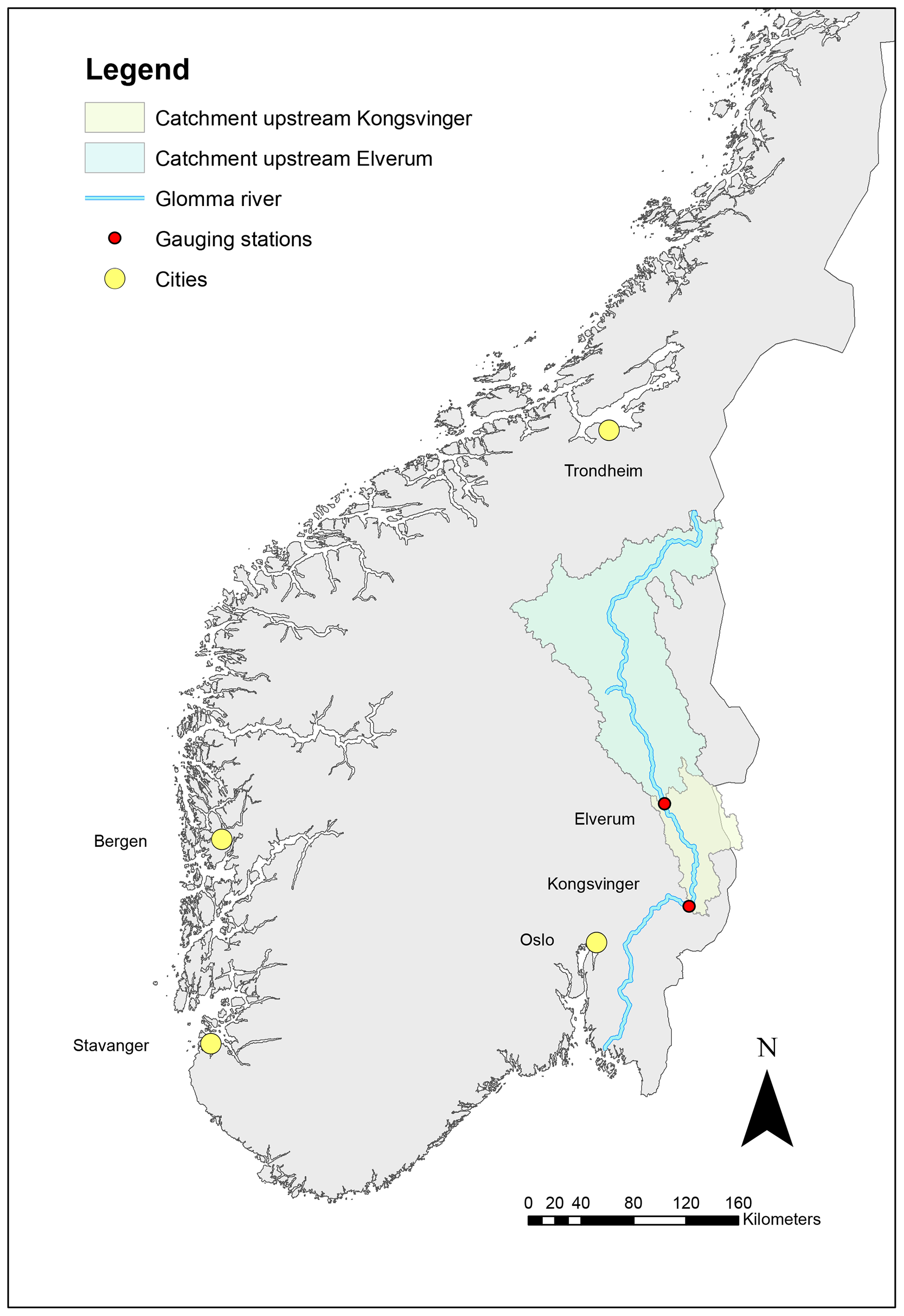
Figure 1The location of the streamflow gauging station at Elverum used for flood frequency analysis and the site for paleodata collection close to Kongsvinger.
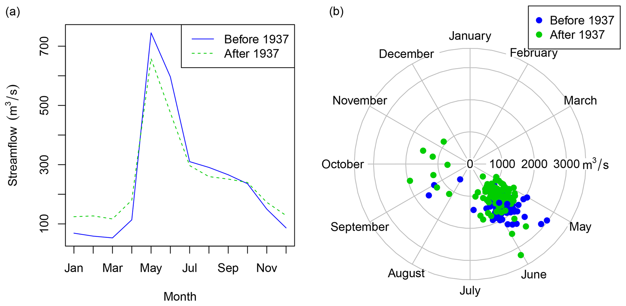
Figure 2Seasonality of Glomma's monthly streamflow (a) and annual maximum floods (b) at Elverum. The dampening of floods after 1937 is explained by upstream dam building.
The catchment has several hydropower reservoirs with a total regulation capacity presently around 10 % of the average annual runoff. The first reservoir was built in 1913, and since 1937 this and other reservoirs have resulted in decreased flood sizes (Pettersson, 2000). The monthly flows during winter have increased and most flood peaks have decreased since 1937 (Fig. 2). The catchment has undergone noteworthy land-use changes during the last 400 years. In the 17th to 19th centuries, the forest areas were reduced due to mining, timber export, and farming practices. Since the beginning of the 20th century, the forest-covered areas have increased slightly, whereas the timber volume has increased substantially, mainly due to farming and forestry practices, e.g. reduced grassing of domestic livestock and forestation (Grønlund et al., 1999).
2.2 Study site for paleodata
To establish a flood record covering most of the Holocene (<11 700 years, Walker et al., 2009), two sediment cores were retrieved at 16 m water depth from Flyginnsjøen (UTM: 33V 0337459 6670202) located close to Kongsvinger, around 80 km south of Elverum as the crow flies (Fig. 1). A detailed map of the study area is shown in Fig. 3, and a conceptual model of the lakes involved, flood water levels, thresholds, and flood pathways is shown in Fig. 4. During normal conditions, water flows from Tarven and Vingersjøen (catchment area 72.0 km2) into Glomma. When the streamflow in Glomma exceeds 1500 m3 s−1, the flow direction reverses, and around 1 %–2 % of the water flows from Glomma and over to Vingersjøen and further into Tarven and Flyginnsjøen, leaves the Glomma catchments, and follows the Vrangselva River across the border to Sweden (Pettersson, 2001). These bifurcation events enable flood water from Glomma to reach Flyginnsjøen, where part of the suspended sediment load is deposited. This is in stark contrast to “normal conditions” for the lake, when the minerogenic sediment delivery is marginal compared to the organic material, as outlined below. The repeated increase in discharge during floods remobilizes readily available sediments – originating mainly from the last deglaciation – and allows for the subsequent deposition of fine-grained minerogenic material. A bathymetric map of Lake Flyginnsjøen and the coring sites which were chosen at the deepest part of the lake, close to the inlet, is shown in Fig. 5. Note that the inlet during bifurcation events is only around 30 m away from the permanent inlet. For addition details about the study site and its surroundings, see the masters theses by Aano (2017), Follestad (2014), and Steffensen (2014).
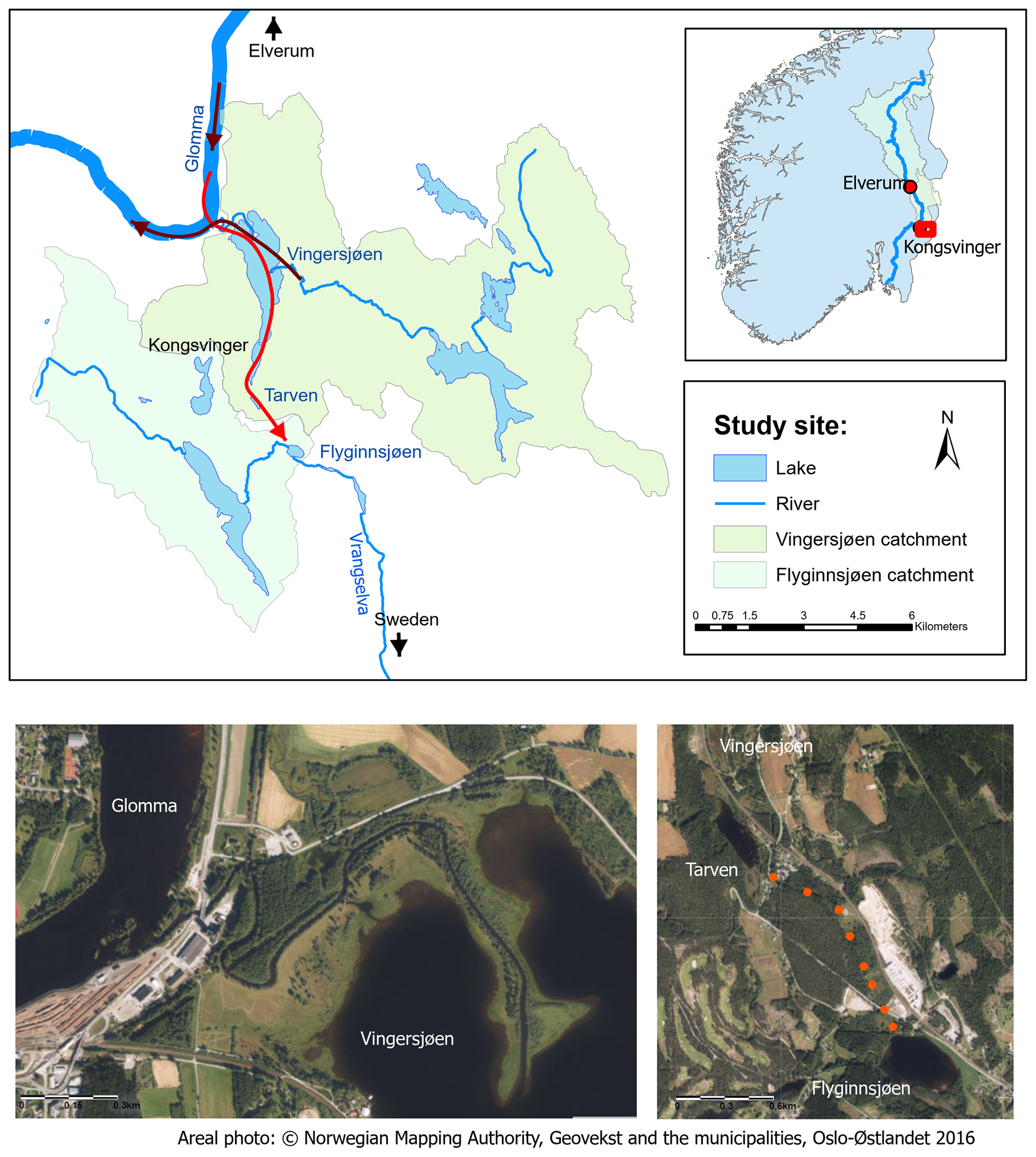
Figure 3Study site for the paleodata. Map: the sediment cores were extracted from Lake Flyginnsjøen. The green arrows indicate the flow direction under normal conditions, whereas the dark red arrow shows the flow direction whenever there is a flood that exceeds 1500 m3 s−1 and bifurcation occurs. Left areal photo: the river between Vingersjøen and Glomma. Under normal conditions the water flows from Vingersjøen into Glomma. Right areal photo: the flood path from Tarven to Flyginnsjøen during bifurcation events is indicated with red dots. Areal photo: © Norwegian Mapping Authority, Geovekst and the municipalities, Oslo-Østlandet 2016.

Figure 4Schematic model of the lakes involved, flood water levels, thresholds, and flood pathways (after Hegge, 1968). The example shows the observed water level exceeding the threshold during the flood in 1967 (2533 m3 s−1) and the normal water level approx. 1 month after the flood event. The dotted red line and arrow show the bifurcation over the threshold, and the red point marks the coring site in Flyginnsjøen. Note that the inlet during bifurcation events is only around 30 m away from the permanent inlet.
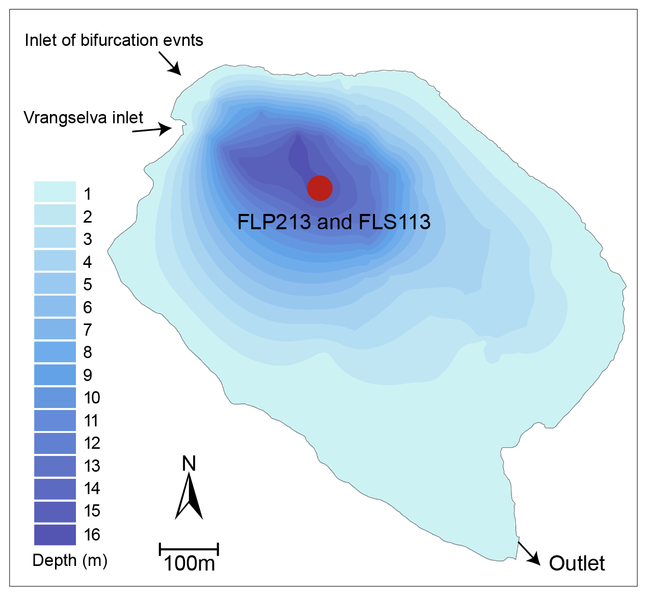
Figure 5Bathymetric map of Lake Flyginnsjøen and the coring sites which were chosen at the deepest part of the lake, close to the inlet. Note that the inlet during bifurcation events is only around 30 m away from the permanent inlet.
3.1 Systematic flood data
Annual maximum flood at Elverum (station number 2.604) for the period 1872–1936 was used for the flood frequency analysis. For this period, we assumed that the flood data were not significantly affected by river regulations (Pettersson, 2000). The mean annual flood for the period 1937–2019 is 1362 m3 s−1. A Wilcoxon test indicates that the difference in the mean value is significant with a p value < 0.01 for the zero hypothesis (i.e. no difference in mean values between the two periods). The modern observations are shown in Fig. 6 together with the known historical floods as well as annual maximum daily floods from the period after 1937, when we observe a minor decrease in average flood size after 1937.
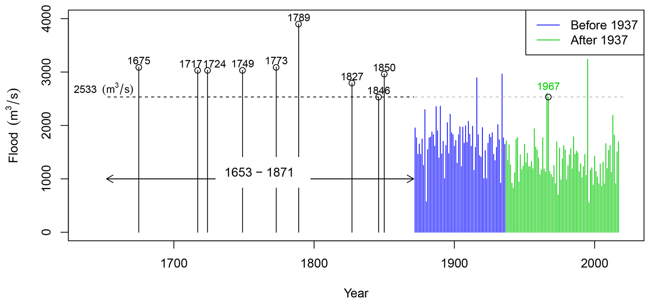
Figure 6Systematic and historical flood data at Elverum. The systematic data from 1872 to 1936 were used for flood frequency analysis. After 1937, the floods are dampened by river regulations. The flood in 1967 reached 2533 m3 s−1 and was used as a threshold for the historical floods. The period for historical floods lasted from 1653 to 1871. The CE 1789 flood known as Stor-Ofsen in Norway stands out in this record.
3.2 Historical flood data
Historical flood information back to 1675 is available as water levels marked at a flood stone in Elverum, located close to Klokkerfossen (“fossen” meaning waterfall) at the Norwegian Forest Museum (Fig. 7 and Tables 1 and 2). Table 1 lists the water levels and discharges for floods exceeding the 1967 flood marked on the flood stone which was erected in 1968. The water levels were carved into the stone in 1969 based on recommendations from NVE (Hegge, 1969); the 1995 flood was added later. There is another flood stone nearby at Grindalen (also shown in Fig. 7). It was erected as early as in 1792 in order to remember the floods of 1773 and 1789, which were large indeed.
Table 1Water levels at Elverum gauging station and at the flood monument from Hegge (1969). The various streamflow peaks are constructed based on the rating curve at gauging station 2.119 and rating curve period 1881–1970. The large floods in 1966, 1967, and 1995 were not included in this study. The flood events in italics are from the period with systematic streamflow measurements.

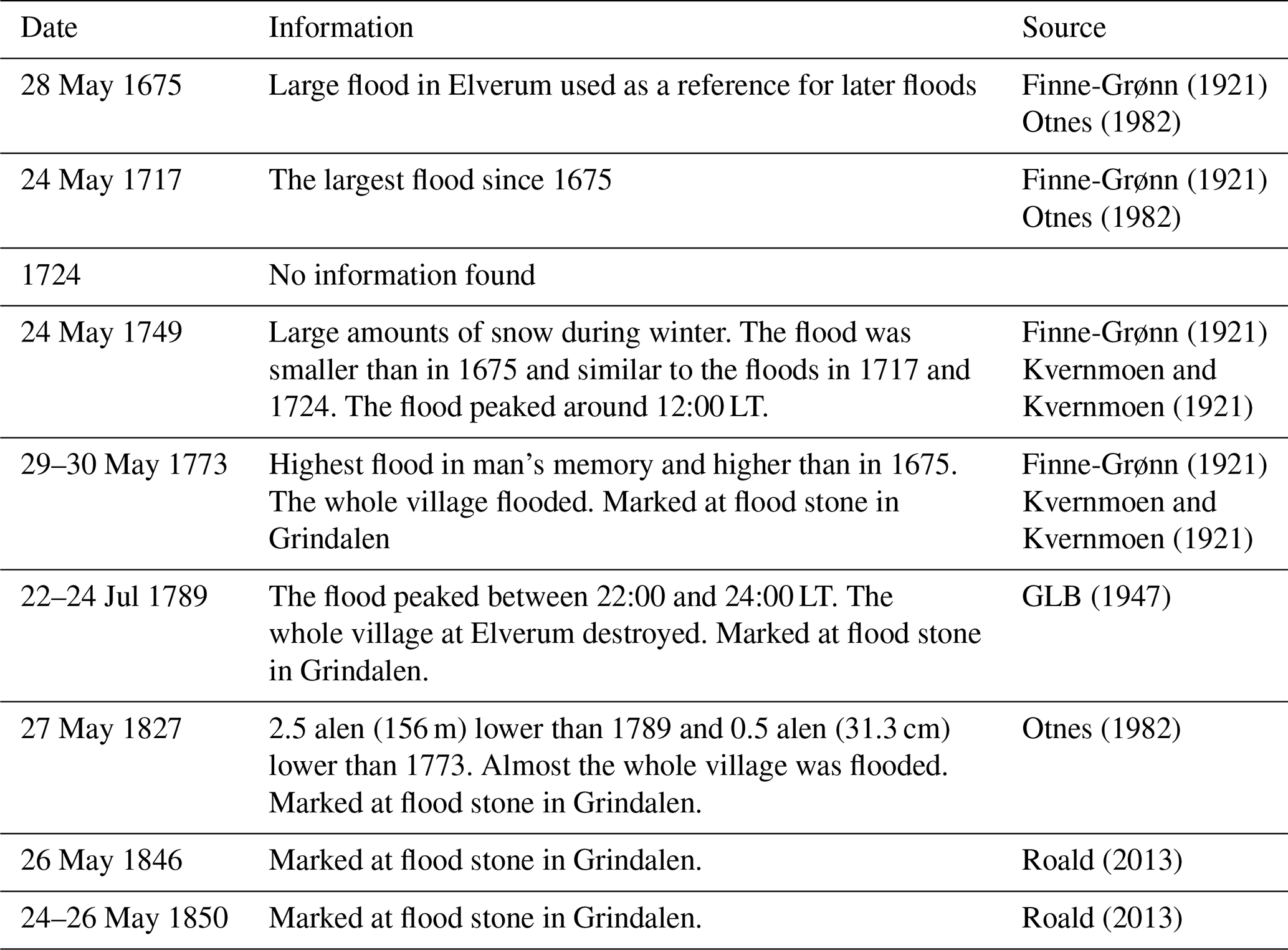
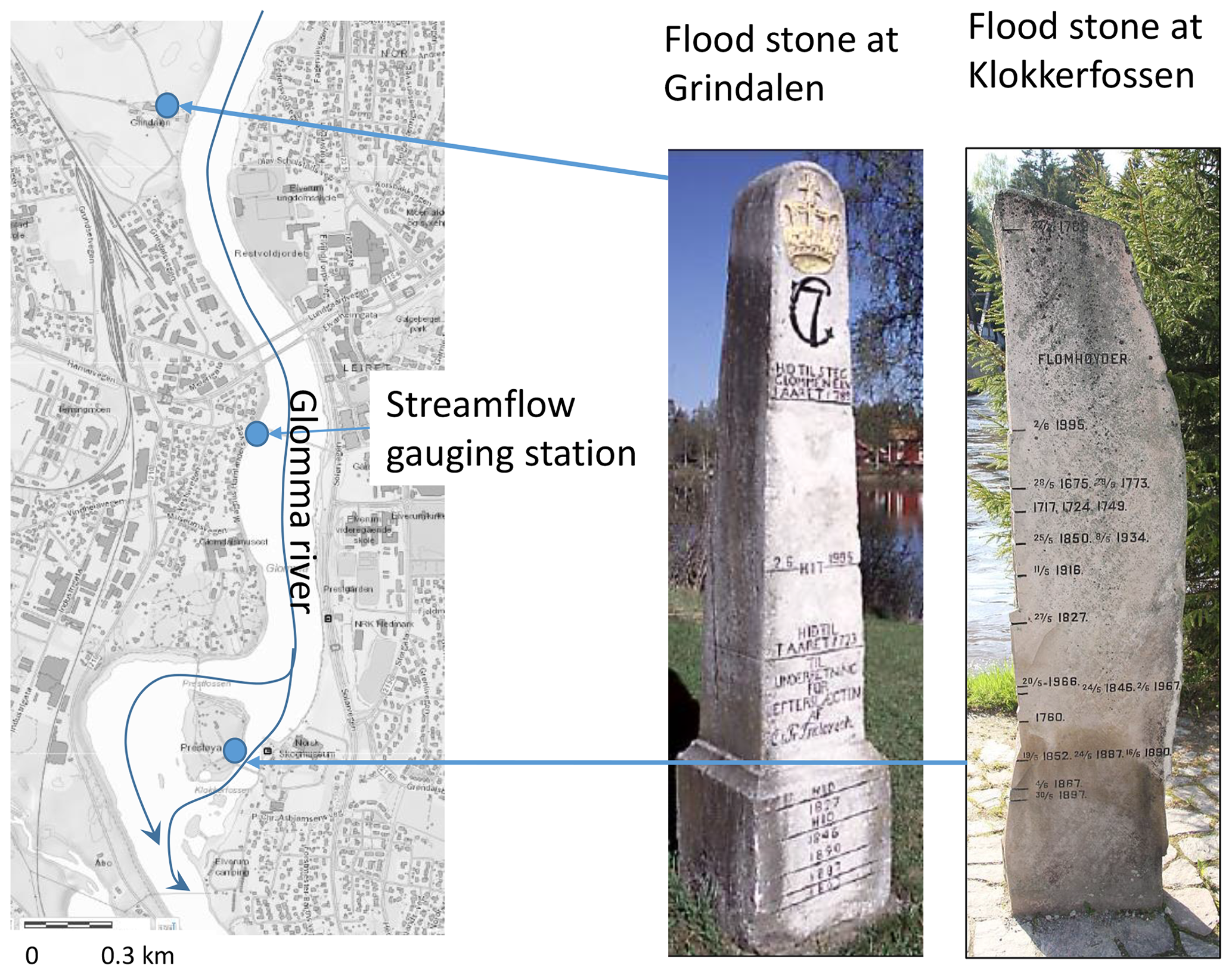
Figure 7Map on the left shows the locations of the flood stones and the gauging station at Elverum (left, created at https://atlas.nve.no/Html5Viewer/index.html?viewer=nveatlas#, last access: 18 November 2020). Pictures to the right show the flood monuments at Grindalen (middle, photo: N. R. Sælthun) and Klokkerfossen at the Norwegian forest museum (right, photo: Ø. Holmstad).
The flood stone at Grindalen is 2 km upstream of the flood stone at Klokkerfossen, with the streamflow gauging station at Elverum in the middle. A waterfall at Klokkerfossen is the controlling profile for the water levels at all three locations. Hegge (1969) developed relationships between water levels at the Elverum gauging station and the flood stone at Klokkerfossen shown here in Table 1. The water levels at the Elverum gauging station were transformed to discharges by using the local rating curve, which assumes that the river profile has been relatively stable since CE 1675. In this study, we included all floods exceeding the observed 1967 flood peak at 2533 m3 s−1 in the flood frequency analysis. By following this approach, we are confident that we only included information on all floods exceeding a specific flood level.
Table 2 summarizes the available historic information and important sources for these floods. The floods in 1675, 1717, and 1749 are all described in Finne-Grønn (1921) and Otnes (1982), whereas information for the flood mark in 1724 is not found in any written source. Detailed information on water levels for floods prior to 1773 was estimated in the absence of historical data. The water levels in 1773, 1789, 1827, and 1846 are all engraved in the flood stone in Grinsdalen and employed here as a basis for calculating the water level at the Elverum gauging station and also for the flood stone at Klokkerfossen. Having said that, we still included all flood water levels listed in Hegge (1969). More information on the historical flood of the Glomma River and at Elverum is provided by Finne-Grønn (1921), Otnes (1982), and Roald (2013). During the period 1675–1870, we see that eight floods exceeded the observed 1967 flood peak at 2533 m3 s−1. The 18th century has a large number of floods at this location. All floods occurred in late May, with the notable exception of Stor-Ofsen in 1789, which occurred in late July.
The largest historical flood in this region was Stor-Ofsen, which took place on 22–23 July 1789 when peak discharge reached 3900 m3 s−1 at Elverum (GLB, 1947), being only slightly smaller than our estimate (see Table 1). Numerous catchments in eastern Norway flooded at the time, resulting in 61 fatalities and destruction of infrastructure, farms, and crops. The economic losses were extraordinary and, in the aftermath of the flood, around 1500 farms got tax reduction (Otnes, 1982).
Prior to Stor-Ofsen, there was a substantial amount of snow in the mountains, deep soil frost, and rainfall that had saturated the soil. During the actual flood event, warm and humid air masses from the south-east were blocked by colder air masses in the north-west, resulting in high rainfall over the entire region. The rainfall intensity peaked on 22 July. The flood started on 21 July in small brooks and culminated the following day (Østmoe, 1985). The main rivers at the bottom of the valleys rose to unprecedented levels, and the flood was also accompanied by numerous landslides. The water levels of this flood are known from several markings cut into rocks, and many flood levels were later transferred to monuments erected at locations near the major rivers (Engeland et al., 2018; Finne-Grønn, 1921; Otnes, 1982; Roald, 2013).
Bifurcation events
Descriptions of bifurcation events and lists of estimated flow volumes in Glomma at Kongsvinger are found in Aano (2017), Pettersson (2001), Hegge (1968), and Reusch (1903). From 1851 to 2013, 79 events in 77 different years were recorded. In 1957 and 1987 there were bifurcation events both in the spring and in the autumn; 4 of the 79 events occurred during the autumn. For the interval between 1953 and 2013, the same period that is covered by FLS113, there were 22 bifurcation events. The transferred volume for the period 1851–2013 is presented in Fig. 8. The five years with the largest transferred volumes are 1916, 1934 1966, 1967, and 1995, with corresponding peak floods at Elverum yielding 2892, 2963, 2600, 2533, and 3238 m3 s−1 respectively. Note that there is a strong statistical correlation (rsq = 0.94) between transferred volume and the maximum transferred discharge. In addition to actual discharge of the individual floods, the duration of each bifurcation event determines the total volume. The estimated peak bifurcation discharge in 1995 was substantially smaller than the estimate for 1916, despite the fact that the water level in Glomma was somewhat higher in 1995 (Pettersson, 2001). Possible explanations for this minor discrepancy are that increased vegetation and/or a local road bridge have reduced the capacity of the intermittent water course. The number of events has decreased since around 1930, mainly due to construction of hydropower reservoirs.
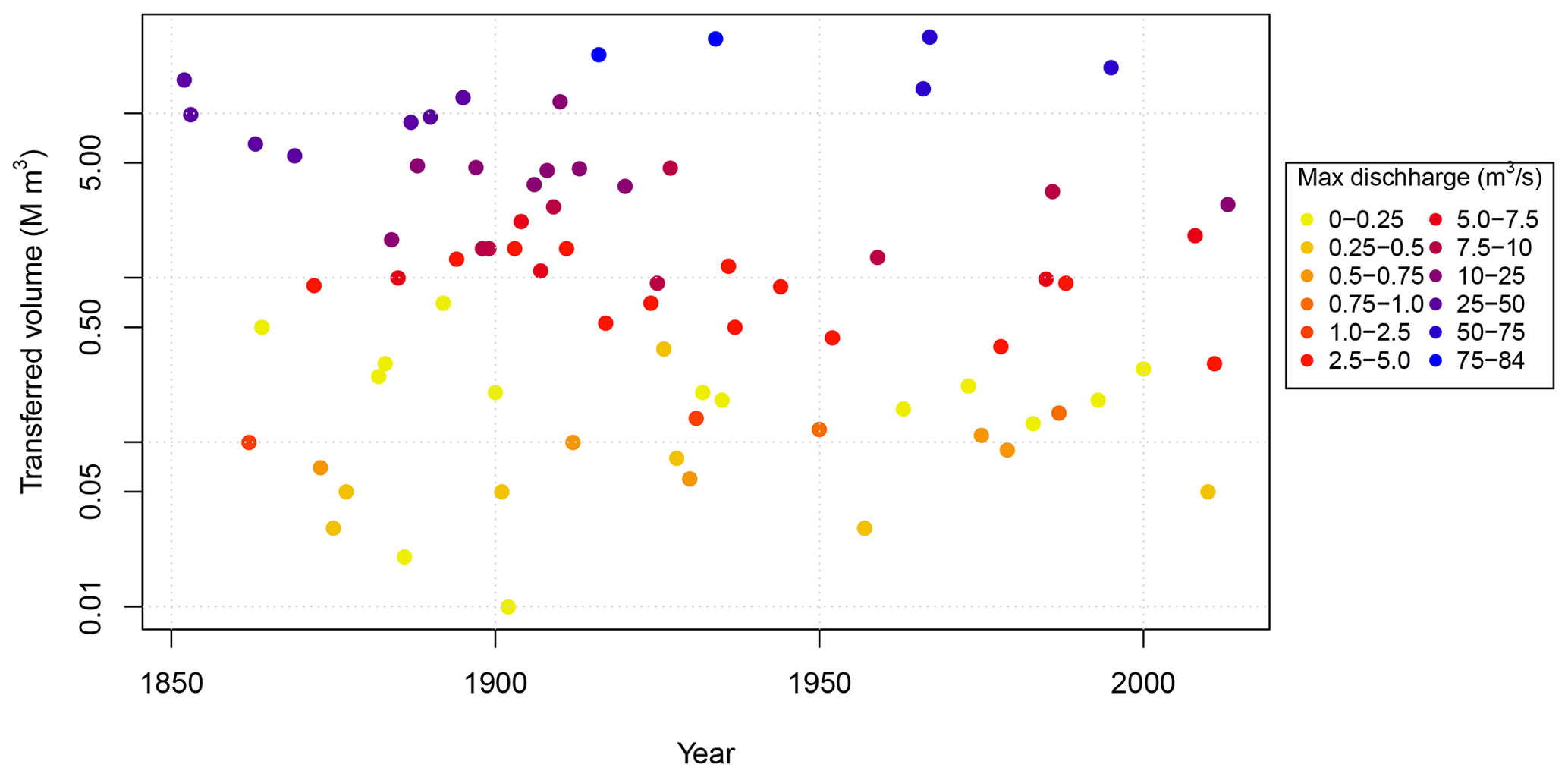
Figure 8Transferred volume (M m3 s−1) and maximum discharge (m3 s−1) indicated by colour for bifurcation events at Kongsvinger. Estimates are obtained from Aano (2017), Pettersson (2001), Hegge (1968), and Reusch (1903).
3.3 Paleohydrological flood data from lakes
Identification of sediment layers
Two sediment cores were retrieved from Flyginnsjøen in 2013 (see Sect. 2.2). Coring sites shown in Fig. 5 were selected at the deepest part of the lake based on a bathymetric survey of the lake using a Garmin Fishfinder echo sounder. A 516 cm long sediment core was retrieved using a 110 mm diameter piston corer (FLP213) (Nesje, 1992). Since the piston corer may disturb sediment layers in the upper 15–20 cm, an HTH gravity corer (FLS113) (Renberg and Hansson, 2008) was used to retrieve a 18 cm core of the youngest sediments. Samples of 1 cm3 were extracted at 0.5 cm intervals from the sediment cores, dried overnight at 105 ∘C, and weighed to measure dry-bulk density (DBD) (Blake and Hartge, 1986). The same samples were subsequently burned at 550 ∘C to measure the weight loss on ignition (LOI) as an estimate of the organic matter content (Dean, 1974). Geochemical properties of the sediment cores were measured using a Cox Analytics ITRAX XRF core scanner at 200 µm resolution, running a Cr X-ray tube at 30 kV and 45 mA for 10 s measurements at each step. XRF measurements were normalized against total scatter (incoherent and coherent) to reduce the potential influence of water content. Images of the split core surface were also captured by the ITRAX core scanner, and 8-bit (255 values) black–white (BW) values were obtained from a 75 px wide average along the length of the core at 200 µm resolution using Image J software. A ProCon Alpha Core computed tomography (CT) scanner running at 100 kV, 200 mA for 250 ms was used to generate 3D X-ray imagery of FLS113 with a voxel resolution of 80 µm. CT data were reconstructed using a ring artefact and median filter in the Volex CT Offline software (ProCon X-ray GmbH) and visualized in Avizo Fire 9.1 (FEI) software. The CT data are given as 16-bit (65 636 values) greyscale values, interpreted as indicating relative densities due to a minimal photoelectric effect at 100 kV (Wellington and Vinegar, 1987) and extracted at 80 µm resolution through a centreline of the FLS113 sediment core. MS was measured on the surface of the split sediment cores at 2 mm sample intervals with a Bartington MS2E point sensor using the CoreSusc MkIII core scanner.
The area between Vingersjøen and Flyginnsjøen (Fig. 4) is rich in glaciofluvial deposits easily remobilized whenever floods occur. Bifurcation events in Glomma cause precisely such a fundamental change in the erosion regime in this area, causing river flooding in a normally dry area (see Sect. “Bifurcation events”). The following calculations and interpretations are thus based on the assumption that bifurcations events can be recorded as a marked increase in minerogenic input to Lake Flyginnsjøen, redeposited from the pre-existing glaciofluvial deposits in the catchment.
To quantify the frequency of such events, a local peak detection algorithm was applied to parameters sensitive to changes in minerogenic input. Flood deposits were defined as peaks in the measured parameters where (i) the measured concentration is higher than the two surrounding values, (ii) the difference between the peak and the lowest value within a specified time window (w) exceeds a specified threshold h1, and (iii) the difference between the peak and the lowest value at each side of the peak (within the time window) exceeds a specified threshold h2, where h2<h1. Each peak should be separated by at least 9 months. We chose a 9-month window since this catchment has one major flood event per year, typically occurring in May/June. For locations with more frequent floods, a smaller time window could be more appropriate.
To produce a Holocene flood record based on the sediment cores from Flyginnsjøen, depth in the core was transformed to time using Bacon age–depth modelling software (Blaauw and Christeny, 2011) (see Sect. 4.1.1), and frequency of events in a 50-year moving window was quantified. In order to test to what extent the lake sediment records reproduce modern and historical observations, identified flood layers were compared with instrumental streamflow data.
3.4 Flood frequency modelling
3.4.1 Stationary flood frequency modelling
A generalized extreme value (GEV) distribution was invoked to establish a flood frequency model for floods at Elverum. The GEV distribution is shown to be a limiting distribution for block maxima (Embrechts et al., 1997; Fisher and Tippett, 1928; Gnedenko, 1943):
where m is a location parameter, α a scale parameter, and k a shape parameter. We estimated the parameters using a Bayesian approach. Their posterior density π* was calculated as
where π is the prior and l(x|m, α, k) is the likelihood of the observation vector x given the parameters m, α, k. The denominator makes the integral under the probability density function (pdf) equal one.
We used non-informative priors for the location and scale parameters (i.e. the location parameter and the log-transformed scale parameter were uniform). A normal distribution with standard deviation 0.2 and expectation 0.0 was used as the prior for the shape parameter k, inspired by Coles and Dixon (1999), Martins and Stedinger (2000), and Renard et al. (2013).
The likelihood for the systematic data is (see Gaál et al., 2010; Stedinger and Cohn, 1986)
where f(xi) is the probability density function for the GEV distribution with the parameter values m, α, k evaluated for the observation xi. For historical and paleo floods, it is assumed that all gj floods exceed a threshold x0,j for the period j where duration hj is known. The likelihood of hj−gj number of floods not exceeding x0,j during the period hj is given as
where F is the GEV distribution given in Eq. (1).
We also need to include available knowledge on floods exceeding x0,j. In the simplest case we know only that gj floods exceeded x0,j; if so, likelihood can be written as
Alternatively, we might know that the floods that exceeded x0 took place within an interval defined by an upper xU and lower xL limit:
And, in an optimal scenario, we know the exact magnitude of all floods exceeding x0,j:
The total likelihood is given as a product of the three major likelihood terms:
where J is the number of sub-periods with specific perception thresholds.
The posterior distribution of the parameters was estimated using a Markov chain Monte Carlo (MCMC) method implemented in R package nsRFA (Viglione, 2012). To estimate return levels, we used the posterior modal values of the parameters. It poses a challenge to set the perception threshold x0 and length of the historical floods h, i.e. for which period the listed floods represent all floods above the threshold. A simple rule is to set the perception threshold to the lowest observed historical flood value in the historical period. The length of the historical period was decided using the average spacing approach as recommended by Engeland et al. (2018) and Prosdocimi (2018).
3.4.2 Plotting position
The plotting positions provided by Hirsch and Stedinger (1987) that build on the Cunnane plotting position (Cunnane, 1978) were used to plot the empirical distribution of the observations. The exceedance probability pi of xi with rank i from a data set with t historical floods representing the historic period h and s systematic floods with e extraordinary floods is given as
where i is the rank, l is the number of extraordinary floods (), and n is the length of the period for which we have information on floods (note that ).
3.4.3 Non-stationary flood frequency modelling
We applied a simple approach to get an estimate of the non-stationary 200-year flood during the recent 1000-year one using the paleorecord. In a first step the parameters m′, α′, and k′ in the GEV distribution were estimated using the systematic flood observations. Then we estimated the flood quantiles as
Note that by replacing F with in Eq. (10) we could calculate the flood quantiles for the return period T.
From the sediment core we estimated a time series of the probability of exceedance wt of the threshold u for each year t by calculating the exceedance rates wt as the mean number of excesses in a sufficiently large moving window. Further, we assumed that the observed non-stationary exceedance rate influenced both the location and scale parameters with a common factor rt. From Eq. (10) we found that
Since the threshold v and the exceedance rate wt are known, the factor rt can be estimated as
The T-year flood for time t can then be estimated as
4.1 Flood variability from the lake sediment cores
The shortest core (FLS113) is 18 cm long and represents the period 1953–2013 (see Fig. 11). The longest core (FLP213) is 516 cm long and represents the period approximately 0–10 300 years before present (present = 1950) (see Table 5 and Fig. 11).
FLP213
The results from the XRF scan (Ti∕total scatter, Ca∕total scatter, and K∕total scatter) and the greyscale value (BW) from a photo of the core are shown as a function of depth in Fig. 9 together with a photo of FLP213. The core consists of a dark brown gyttja with preserved macro fossils including leaf fragments. This gyttja, carrying a low minerogenic content, is referred to here as “the background signal” which is characterized by its dark colour (BW < 30), high LOI (30 %–40 %), low DBD (<0.3 g cm−3), and magnetic susceptibility (MS) with values close to zero (<5 SI × 10−5). Moreover, it returns low K∕total scatter (<0.03), Ti∕total scatter (<0.03), and Ca∕total scatter (<0.03). Interspersed in this “organic slush” there are narrow (millimetre-scale) light grey (BW 40–170) minerogenic layers with LOI lower than 20 %, relatively high density (DBD 0.5–1.0 g cm−3), higher than average MS with peaks at 15–20 SI × 10−5, as well as peaks in K∕total scatter (0.1–0.9), Ti∕total scatter (0.1–0.4), and Ca∕total scatter (0.1–0.7). At 33.5–18.0 cm depth in the core there is an anomalous thick minerogenic layer with LOI at <2 %, DBD at 1.6 (g cm−3), MS at 98 SI × 10−5, and very high K/∕total scatter (0.6), Ti∕total scatter (0.4), and Ca∕total scatter (0.7).
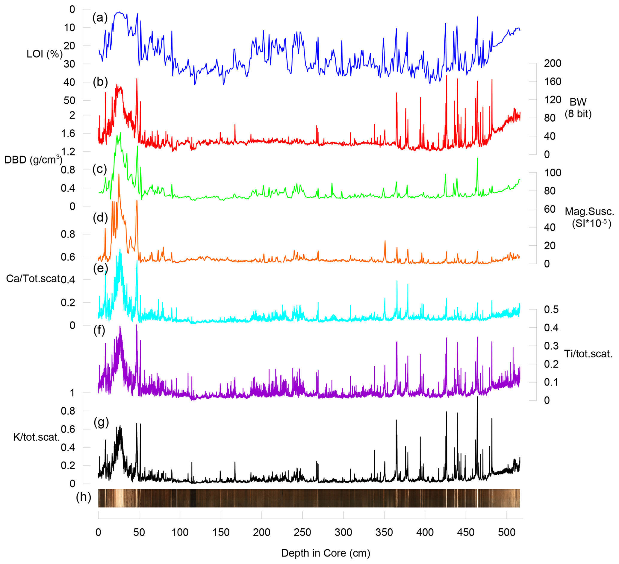
Figure 9Results from measured parameters in FLP213. (a) Loss on ignition (LOI, %) indicated content of organic matter in the core and is plotted on an inverse scale (blue). (b) BW (red) shows the 8 bit (0–255) black–white values extracted from a photo of the core surface where 0 is black. (c) Dry bulk density (DBD) is plotted in unit g cm−3 (green). (d) Magnetic susceptibility (orange) is plotted as SI × 10−5 as magnetic susceptibility is a dimensionless parameter. (e–g) XRF data (K, Ca, and Ti) are normalized against total scatter to reduce the potential effect of water content. (h) RGB photo of core.
The correlation matrix (Table 3) shows strong (and significant) correlations between K∕total scatter, Ti∕total scatter, Ca∕total scatter, MS, and BW. The weakest correlation is 0.74 between MS and BW, which is still very high. LOI is, as expected, negatively correlated with all the other measured variables. We suggest that the main process explaining the relationships between these parameters is driven by the on–off signal related to transport of minerogenic material to Flyginnsjøen during bifurcation events.
Table 3Correlation between measured parameters in FLP213 (in bold) and FLS113 (in italic). LOI, BW, DBD, MS, and the XRF data (K, Ca, and Ti) were measured in FLP213, whereas CT greyscale, MS, and the XRF data (K, Ca, and Ti) were measured in FLP113. LOI (%) indicates content of organic matter in the core; BW is the 8-bit (0–255) black–white values extracted from a photo of the core surface where 0 is black. CT greyscale is a 16-bit number indicating relative densities of the core; DBD is given in unit g cm−3 (green). MS is measured as SI × 10−5 (it is a dimensionless parameter). XRF data (K, Ca, and Ti) are normalized against total scatter to reduce the effect of water content. All correlations are significantly different from zero.

FLS113
This core shows dark organic gyttja with light grey minerogenic layers, similarly to FLS213. The minerogenic layers yield high values of K∕total scatter (0.2–0.8), Ca∕total scatter (0.1–0.4), and Ti/∕total scatter (0.1–0.2) as well as a slight increase in MS (>6 SI × 10−5) (Fig. 10). CT data show that the light grey layers are of high density and reveal numerous thinner layers not visible on the photo or in the lower-resolution XRF and MS data. Slight offsets in the positioning of layers in the CT imagery and optical photo occur due to the fact that the layering is not entirely horizontal.

Figure 10Results from high-resolution analysis of core FLS113. (a) shows a 3D CT visualization of high-density layers (white) in the core. (b) The 2D slice is an 80 µm thick slice from the middle of the sediment core. (c) The optical photo is an RGB photo of the surface of the halved sediment core. The CT greyscale plot (d) shows an 80 µm greyscale variability along a line through the middle of the sediment core. MS (e) is plotted as SI × 10−5 as magnetic susceptibility is a dimensionless parameter. (f–h) XRF data (K, Ca, and Ti) are normalized against total scatter to reduce the effect of water content.
Correlation coefficients between CT greyscale values, MS, K∕total scatter, Ca∕total scatter, and Ti∕total scatter in FLS113 are all over 0.59 and significantly larger than zero. The strongest correlation is seen between K∕total scatter, Ca∕total scatter, and Ti∕total scatter (Table 3). The somewhat weaker correlation with MS and CT greyscale and the fact that CT imagery shows layering (e.g. 11–12 cm depth in the core) not picked up by the other data (Fig. 10) can partly be explained by slight offsets in the positioning of layers between the different scans as well as differences in sampling resolution. The strong correlations and general picture of layered intervals yielding high values, however, indicate that one dominating factor “controls” the variability, providing further support for the interpretation that transport of minerogenic material to Flyginnsjøen during bifurcation events is the main process.
4.1.1 Age–depth models
To establish an age–depth relationship for the cores, sediments were subjected to lead dating (210Pb) of FLS113 and radiocarbon dating (14C) of FLP213. Measurements were performed by the Environmental Radioactive Research Center at the University of Liverpool (Appleby and Piliposian, 2014) and Poznan Radiocarbon Laboratory in Poland. The 210Pb and 14C dates used to establish the age–depth models presented in Fig. 11 are listed in Tables 4 and 5. Estimation of age as a function of depth for FLS113 was done using a quadratic term regression model of CRS model calculations of the 210Pb with the 1963 137Cs peak at 16.25 cm depth in the core (Table 4) as a reference point (Appleby, 2001). For FLP213, we used a Bacon age–depth modelling approach (Blaauw and Christeny, 2011) available in R package Bacon. One 14C sample from 51 cm depth in FLP213 was rejected, as this has a stratigraphically reversed age (see Table 5). The age is clearly too old, possibly related to high content of sawdust bringing in a relatively old carbon core at depth in the core. The sawdust may have originated from a saw mill in the catchment at this time. The 15.5 cm thick anomalous layer at 18.0–33.5 cm depth in the core was classified as “slump” in the Bacon model and thus interpreted as an instantaneous event deposit. This layer has a basal age estimate of 1776 CE from the age model and is likely to be related to the historically documented 1789 CE Stor-Ofsen flood event (see Sect. 3.2).
Table 4Fallout radionuclide concentrations and chronology for FLS113 from Flyginnsjøen.

Table 514C dates for FLP213 from Flyginnsjøen. Radiocarbon ages are calibrated using the IntCal 13 calibration curve (Reimer et al., 2013).
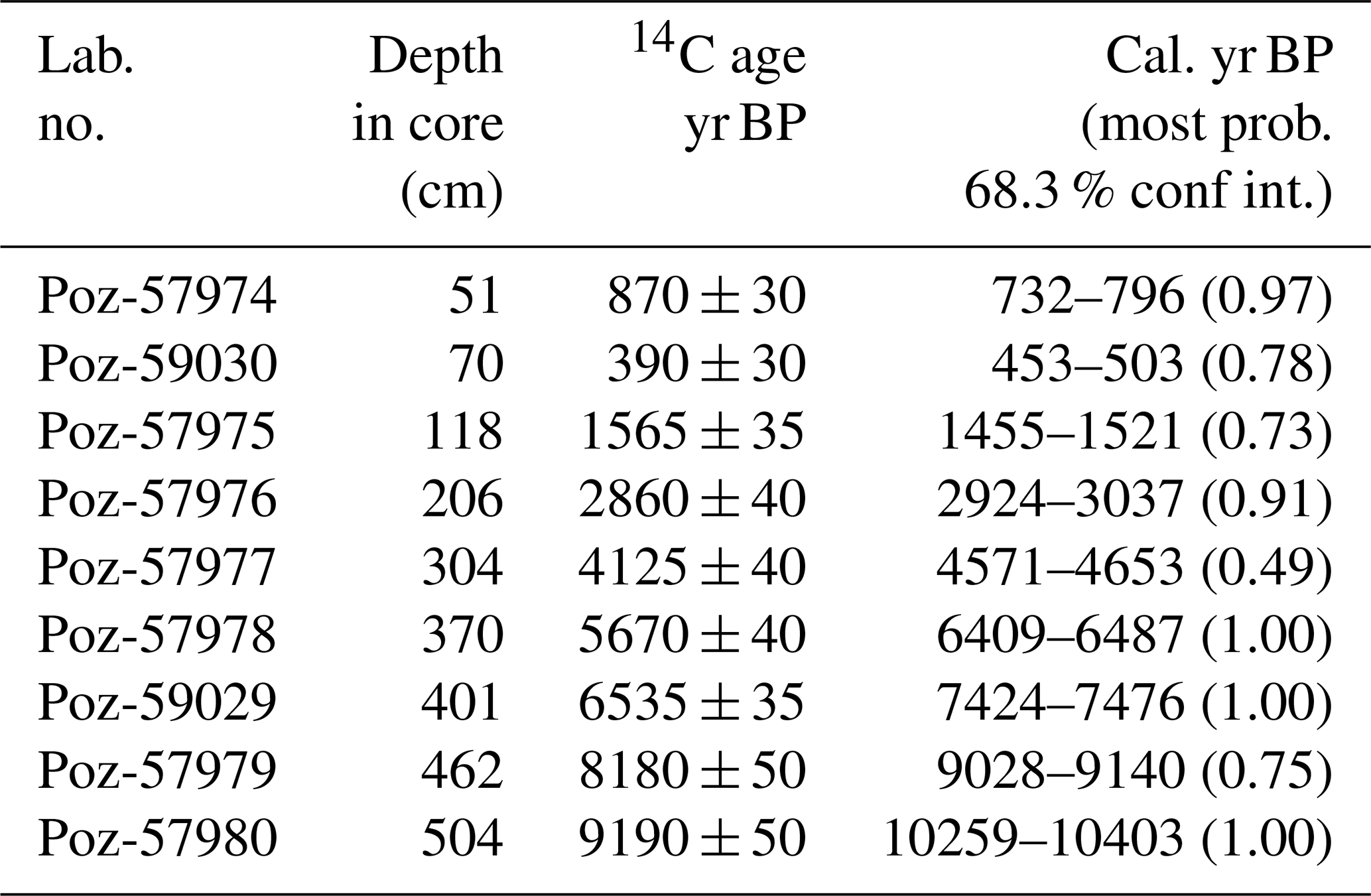
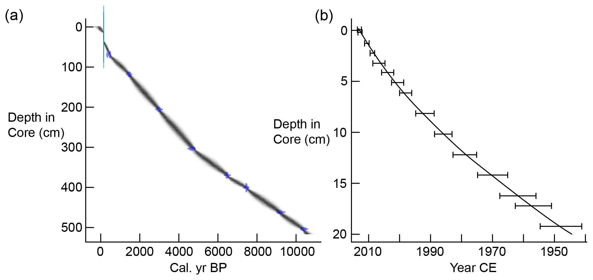
Figure 11Age–depth model for FLP213 (b) and FLS113 (a). Note the step in the FLP213 age–depth model at 33.5–18.0 cm depth in the core related to the Stor-Ofsen flood event in 1789 CE.
4.1.2 Identification of flood layers in FLS113
We used the concentrations of Ti∕total scatter and K∕total scatter from the XRF scan of FLS113 to establish a link between dense, minerogenic sediment layers and the 22 bifurcation events between 1953 and 2013. Note that XRF data (K∕total scatter, Ca∕total scatter, and Ti∕total scatter) correlate strongly with the CT scan (greyscale values) and MS for both FLS113 and FLP213 (Table 3), and this suggests the flood-transported material originates from one source and that this is constant over time. All detected layers are thus interpreted as being related to the same process bringing minerogenic material to Flyginnsjøen. The first step in our approach was to transform the depth of the XRF scan to age using the depth–age model for FLS113. After having identified the flood layers, we used the algorithm described in Sect. “Identification of sediment layers” to identify local peaks in the measured parameter. We used a time window of 1 year and values of 680 and 527 for Ti∕total scatter and K∕total scatter respectively for h1 and which identified 23 local peaks for Ti∕total scatter and K∕total scatter over the same period that we observe 22 bifurcation events. A time series of the bifurcation volumes and the XRF-scan data can be viewed in Fig. 12. Taking into account the uncertainty in the dating (Fig. 11), we see that five of the bifurcation events do not correspond directly to a sediment layer. All three largest flood events were, however, correctly identified, and considering the uncertainties in the age–depth model, this supports our working hypothesis that sediment layers can be used to identify flood events caused by episodes of bifurcation at Kongsvinger.
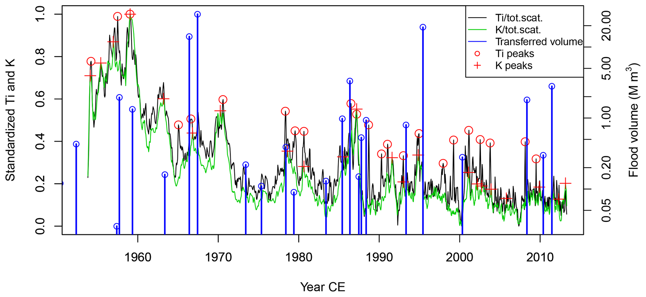
Figure 12Transferred volume of the 23 bifurcation events in the period 1950–2013 CE (in blue) and the 24 identified flood layers (red) identified using XRF scans of Ti∕total scatter and K∕totalscatter for FLS113.
4.1.3 Frequency of flood events during the Holocene
From FLS113 we have established a link between dense, minerogenic sediment layers and bifurcation events. We therefore assumed that the analyses of FLP213 could be used to produce a time series of flood events covering the last 10 300 years. Here we used the local peak detection algorithm presented above to identify sediment layers with high concentrations of K∕total scatter and Ti∕total scatter. Since the uncertainty range in the age estimate is 30 to 50 years, we calculate the average rate of a given flood event within a moving Gaussian time window of 50 years for both Ti∕total scatter and K∕total scatter (Fig. 13). The standard deviation of the estimated flood rate was calculated as , and it was used to assess the 95 % confidence intervals. We see that the flood counts using Ti∕total scatter, K∕total scatter, and BW to a large degree overlap and follow the same Holocene trends, as anticipated due to the high correlation coefficient between the two (see above).
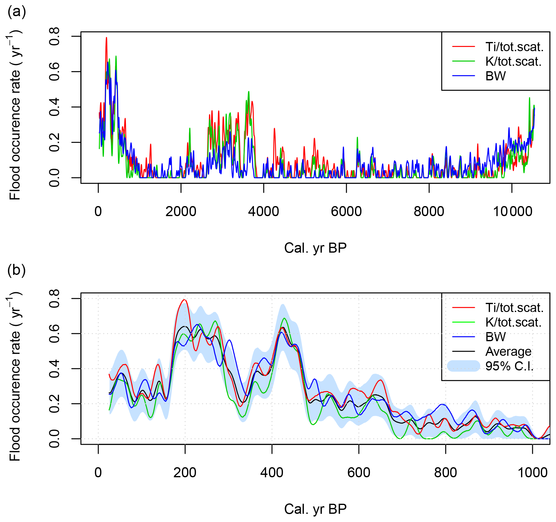
Figure 13In (a), average flood rate per year calculated in a 50-year moving window during the Holocene. In (b), the most recent 1000 years are shown only. Panel (b) also includes a 95 % confidence interval for the average flood rates. The flood rates were identified by detecting local peaks in Ti∕total scatter, K∕total scatter, and BW values.
4.2 Stationarity of flood frequency in the paleoflood data
A key observation in the Holocene flood frequency reconstruction is the large non-stationarity played out across multiple timescales. We observe that there are two major flood-rich periods during the Holocene (Fig. 13a). The first runs from 3800 to 2000 cal yr BP, when it ends abruptly. The second period extends from around 700 cal yr BP up to the present day. Looking at flood frequency over the most recent 1000 years (Fig. 13b), we observe significant internal variability within the flood-rich period. The period with the highest flood rates occurs in the 18th century but also in the 15th century. The data from FLP213 inform us that the flood event in 1789 is truly an anomaly, as is evident from the sheer amount of sediments deposited during this event (no other flood comes close), and it also yields the highest measured values of e.g. density (DBD) as well as magnetic susceptibility (MS) throughout the core (Fig. 9). It is therefore reasonable to assume that the 1789 CE flood was an extraordinary event, making it the largest during the entire time span of the record, i.e. 10 300 years.
Table 6Overview of the three data sources used for flood frequency analysis.
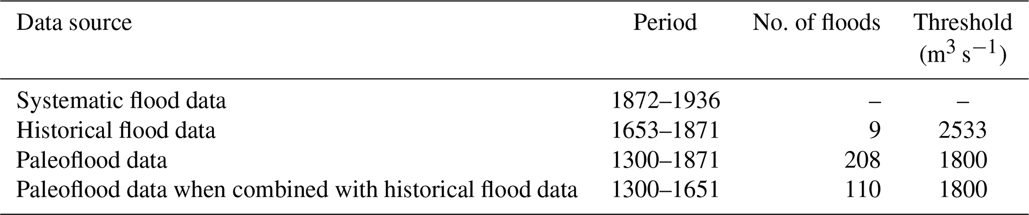
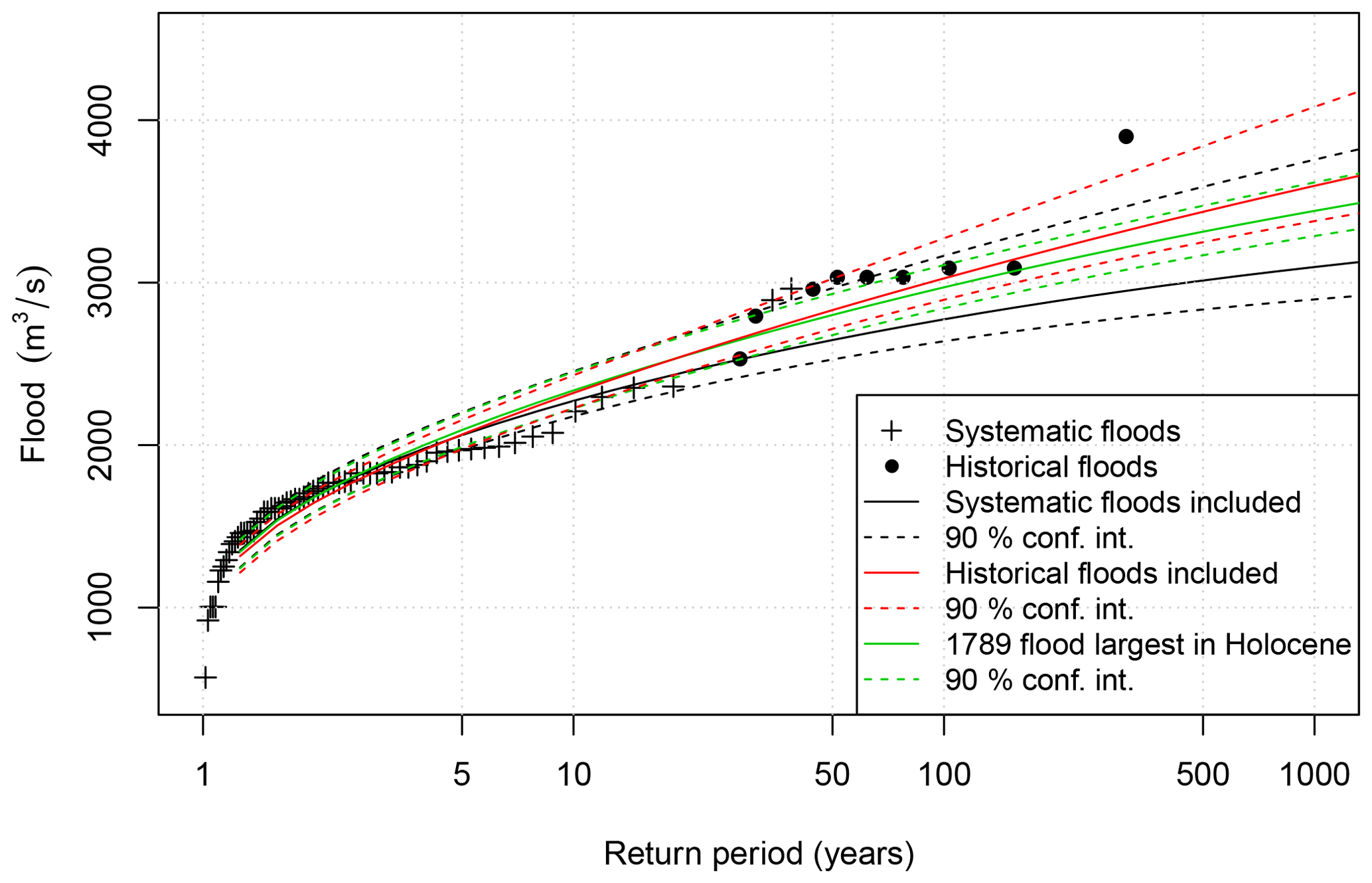
Figure 14The sensitivity of flood frequency analysis to three different combinations of systematic and historical flood data. Annual maximum floods for the period 1872–1836 were used as systematic flood data. Nine historical floods exceeding 2533 m3 s−1 and representing the period 1653–1871 were used as historical floods. Based on the paleorecord, the 1789 CE flood was reweighted to represent a period of 10 000 years. The plotting positions for the systematic and historical floods are based on Hirsch and Stedinger (1987) and explained in Sect. 3.4.2.
4.3 Flood quantile estimation by combining systematic, historical, and paleo flood data
The flood quantiles combining the systematic, historical, and paleo data have been analysed in different but complementary ways. Table 6 provides an overview of the flood information related to the data source and the time intervals they represent. The first step was to estimate the flood quantiles using only systematic data. In the second approach we added all the historical flood data. The smallest historical flood of 2533 m3 s−1 was used as the threshold x0. The length of the historical data period was calculated based on Prosdocimi (2018) and Engeland et al. (2018). Since the average waiting time between the historical floods is 22 years, the start of the historical period was set to be 22 years before 1675 CE (i.e. the year of the oldest historical flood). The historical period ended in 1871 CE, giving h=219 years. The exact sizes of the historical floods (Table 1) were assumed. In the third approach we used the paleorecord as a guide to weigh the historical information. Since the paleorecord indicates that the historical floods in the 18th century occurred in a flood-rich period, we used only the historical flood events from the 19th century. Moreover, the historical flood from 1789 CE was included, and it was suggested that this was the largest flood during the last 10 000 years for the reasons explained above. The results are shown in Fig. 14, and we see that the results are sensitive to the assumption of which period the 1789 CE flood represents.
The next step was to include the paleoflood information in the flood frequency analysis. We did this in two ways: (i) we combined the systematic data and the paleodata and (ii) we combined systematic, historical, and paleo data. For the paleodata we used 1800 m3 s−1 as the threshold x0 since it provided the same number of flood events (i.e. 19 events) from the paleo record and the streamflow observations for the overlapping time period (1891–1950). When we combined the systematic data and the paleodata, we counted 208 flood events representing a period of 572 years (1300–1871 CE). When we combined the systematic, historical, and paleo data, we counted 110 events for a period of 353 years (1300–1652 CE) from the paleodata and used the nine historical floods representing the period 1653–1871. The results are shown in Fig. 15. We see that the estimates are sensitive to historical information. The paleodata did not impact the result to the same degree.
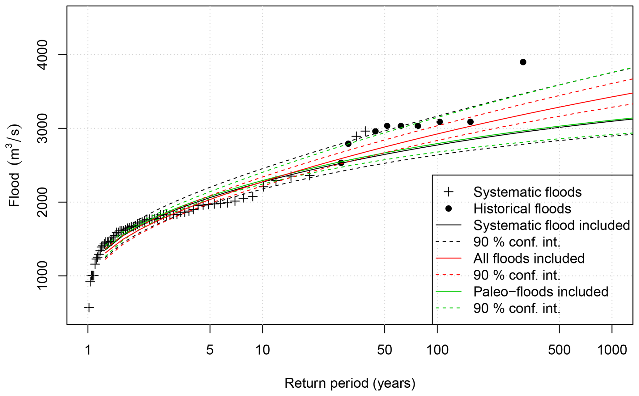
Figure 15The sensitivity of flood frequency analysis to three different combinations of systematic, paleo, and historical flood data. Annual maximum floods for the period 1872–1836 were used as systematic flood data. Paleofloods representing 208 events exceeding 1800 m3 s−1 for the period 1300–1871. When all flood data were combined, the paleofloods represent 110 events for the period 1300–1652, and nine historical floods exceeding 2533 m3 s−1 and representing the period 1653–1871 were used as historical floods. The plotting positions for the systematic and historical floods are based on Hirsch and Stedinger (1987) and explained in Sect. 3.4.2.
To achieve a non-stationary estimate of the design flood, we used the flood occurrence rate presented in Fig. 13 to estimate the 200-year flood in a moving time window as explained in Sect. 3.4.2. We used 1900 m3 s−1 as the threshold v in Eq. (11) since it provided a good agreement between the 200-year flood estimated from the systematic data and the non-stationary 200-year flood for the overlapping period. The results are presented in Fig. 16. We now see that the size of the 200-year flood is non-stationary. During the Little Ice Age (LIA) it was up to 23 % higher than in the present climate, whereas during the period 4000–6000 BP it was around 30 % lower than today.
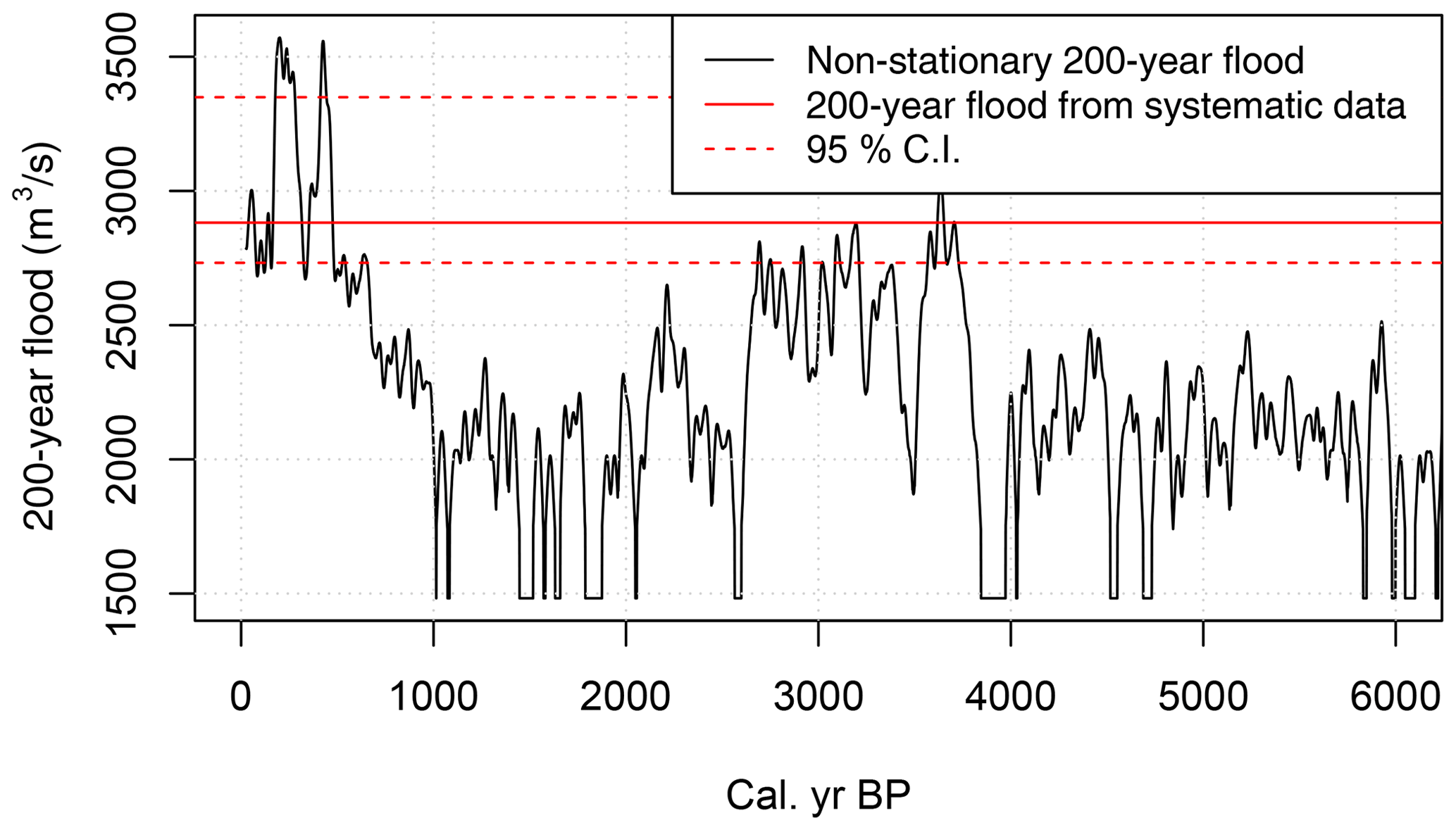
Figure 16Non-stationary estimate of the 200-year flood for the recent 6000 years. The red lines indicate the estimated 200-year flood and the 95 % confidence intervals estimated using systematic streamflow observations.
5.1 The reliability of the historical data and the paleoflood records
The historical data applied in this study are marked as water levels at the flood stone at Elverum, and the associated flood discharges are estimated by Hegge (1969). An assumption for these estimates is that the river profile is relatively stable over the historical period and in particular that the large flood in 1789 CE did not cause any substantial changes. This is a reasonable assumption because, although four large floods occurred between 1781 and 1969 CE, only one rating curve is used for the period. The gauging station was moved around 660 m in 1969.
During the last decade or so lakes across Europe have been studied in detail and high-resolution paleoflood records have been produced from both the lowlands and the highlands (cf. Wilhelm et al., 2018). Unlike many of these studies, we have worked with lakes that only receive flood-delivered sediments whenever the local river (Glomma) exceeds a certain well-known threshold (1500 m3 s−1). This setting tends to suggest that we are working not only with a sedimentary archive that filters out noise, but also one that provides a minimum estimate of the discharge associated with the floods recorded. The flood information extracted from the lake sediment cores, nevertheless, relies on a set of assumptions that is discussed in the following.
The first assumption is that all flood events recorded in Lake Flyginnsjøen are directly related to Glomma. We cannot completely rule out the possibility that minor floods in the local catchment of Flyginnsjøen occurred simultaneously with floods originating from Glomma or even just within the very small catchment surrounding the lake due to local rainstorm events. Given the heavy vegetation cover in the catchment of Flyginnsjøen, its small size, and the low angles of the slopes leading into the lake, we deem the possibility of a local sedimentary imprint to be very low. This is supported by both XRF and MS data. The consistency in bifurcation events causing peaks in concentration in both Ti∕total scatter and K∕total scatter, as well as MS, suggests that the source region for this signal remains the same throughout the record. The most likely source is thus the abundant glaciofluvial material available in the area between Tarven and Flyginnsjøen (see Fig. 4).
A second assumption is that the river channel and landscape geometry controlling the bifurcation events have not changed over the approximately recent 10 000 years to the extent that it alters this interplay between a flooding Glomma and the investigated lake. The current river geometry was shaped by a glacial lake outburst flood (GLOF) some 10 000–10 400 years ago with a peak discharge of more than 106 m3 s−1 (Høgaas and Longva, 2016). This GLOF flushed the valley where Glomma runs and also established the current river channel at Kongsvinger (Pettersson, 2000). Based on Klæboe (1946) and Hegge (1968), the threshold between Vingersjøen and Flyginnsjøen (Fig. 4) is a resilient and stable topographic feature. The intermittent drainage patterns that route water from Vingersjøen to Flyginnsjøen during the bifurcation events may have undergone some changes during the course of time, but it is hard to see how this would directly influence the deposition of flood-delivered sediments to Flyginnsjøen. According to Hegge (1968), the flood events that occurred in 1967 and 1968 CE caused some erosion at the very highest elevation of this intermittent water course. Having said that, these flood events did not cause any major damages to this area (Klæboe, 1946). In recent years, denser vegetation and also the construction of a road bridge has potentially lessened the transfer capacity between the lakes, although we have little or no evidence for this based on what we observe in the lake core.
The resolution of the XRF signal is on average sub-annual, but because of the uncertainty in the age–depth we calculated flood rates, i.e. average number of flood events, for a moving 50-year window. Unlike the findings of Evin et al. (2019), and although the floods are of varying magnitude, there appears to be no systematic relationship between flood sizes and sediment thickness or volume except for the Stor-Ofsen event. This is probably explained by the fact that the sediment transport for individual floods will in part be deposited in the two preceding lakes (Vingersjøen and Tarven) buffering Flyginnsjøen (Fig. 4) but may also indicate that event-specific features such as ground frost or snow cover may regulate sediment availability.
5.2 Non-stationarity in flood records and regional climate co-variability
The paleoflood data presented here document that the flood frequency is non-stationary during the last 10 300 years, being manifested on multiple timescales (Fig. 13). Non-stationarity is typically identified as quasi-cyclic flood-rich and flood-poor periods (for European studies, see e.g. Brázdil et al., 2005; Glaser et al., 2010; Hall et al., 2014; Jacobeit et al., 2003; Kundzewicz, 2012; Mudelsee et al., 2004; Swierczynski et al., 2013), where the flood-rich period may last for 50–60 years (e.g. Glaser et al., 2010). Over the instrumental and historical eras, floods in the Glomma catchment have mainly occurred in late spring (late May, early June) due to the sudden melting of large snow reservoirs following a steep rise in temperatures that often overlaps with persistent rain (Roald, 2013). Under the current climate conditions, the largest floods in the Glomma catchment are caused by (i) high winter precipitation and preferentially cold winters resulting in a large snow storage, (ii) a cold spring followed by a sudden increase in air temperature producing high melt rates, and (iii) large amounts of widespread precipitation combined with snowmelt (Vormoor et al., 2016). Importantly, for these spring-snowmelt-triggered floods, the soils are either frozen and/or already saturated with moisture channeling shallow sub-surface flow and overland flow resulting in a fast discharge response to snowmelt and rain. Based on these observations, we hypothesize that on decadal to centennial timescales, increasing flood sizes can be explained by increasing precipitation, in particular during winter and spring, and cool winter temperatures. Increasing spring and summer temperatures might potentially lead to increasing flood sizes, but this effect depends strongly on the snow storage available for melt.
In Figs. 17 and 18 we compare the flood frequency reconstruction from Flyginnsjøen to several climate reconstructions representing temperature and precipitation on a centennial- to decadal-scale variability. In Fig. 17, the flood frequency is compared to regional summer temperature reconstructions (Moberg et al., 2005), whereas it is compared to local records of glacier variability (upper panel), a flood index (second panel), and local July temperature (third panel) in Fig. 18. No continuous reconstructions of winter precipitation are available for this region; however, the glacier growth in Scandinavia is primarily driven by summer temperatures and winter precipitation, and the reconstructed flood record is therefore compared to glacier variability in Rondane in the upper Glomma catchment. Low values of the flood index produced by Støren et al. (2012) reflect periods with relatively high flood frequency in eastern Norway. We observe co-variability between the reconstructed flood frequency in Flyginnsjøen and several of the climate reconstructions, which may indicate that the non-stationarity of flood frequency is, to a large degree, related to non-stationarities in climate. The data from Flyginnsjøen show, for instance, two distinct intervals with high flood frequency during the LIA, both played out on centennial timescales. Since 1850 there has been a steady increase in summer temperature followed by a reduction in flood frequency. Enhanced flooding during the LIA is observed in other lake studies from eastern Norway as well, including Atnasjø (Nesje et al., 2001), Butjønna (Bøe et al., 2006), Meringdalsvannet (Støren et al., 2010), and also the Grimsa River in the headwater of Glomma (Killingland, 2009).
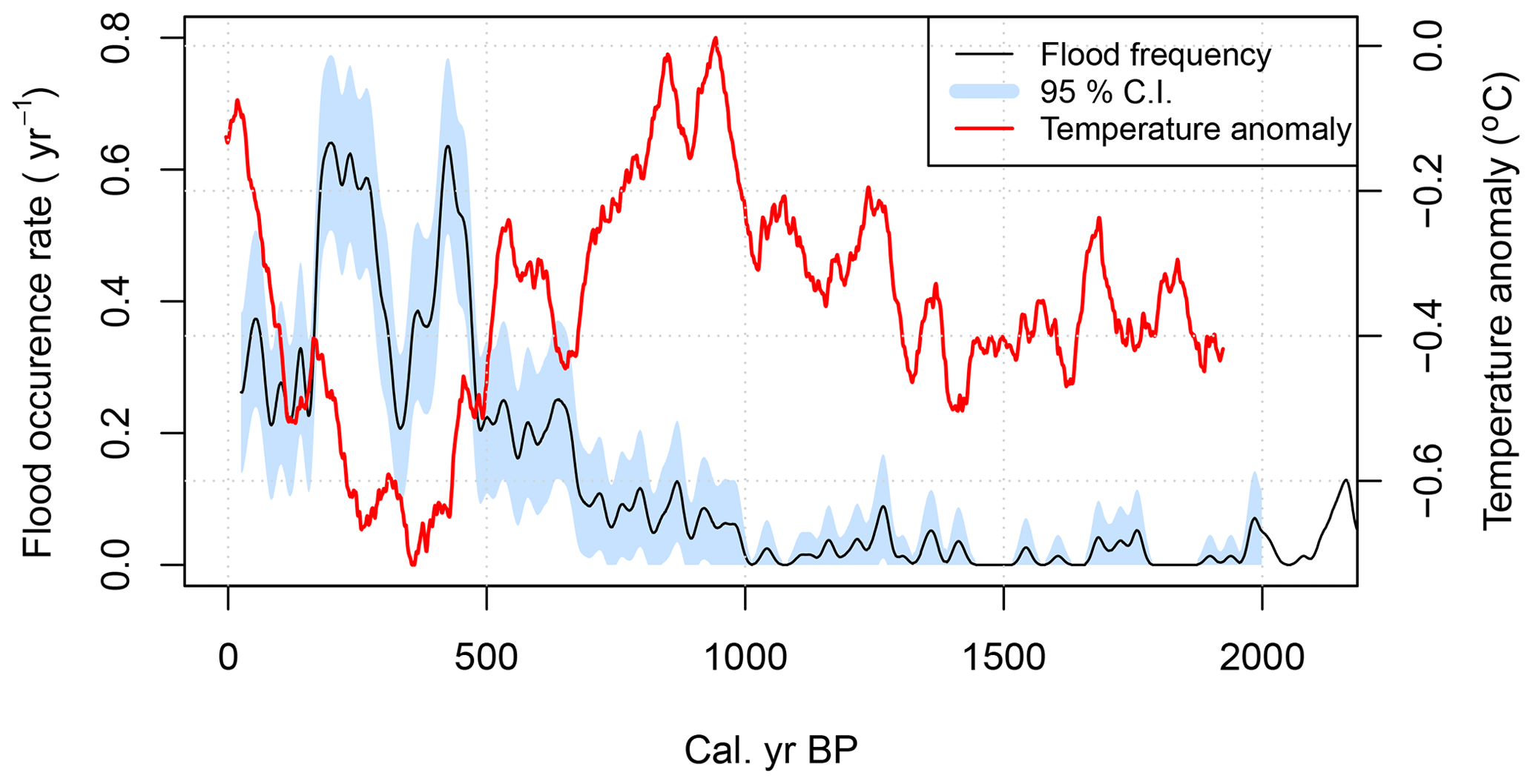
Figure 17Flood frequency in Glomma (blue bars) and 30-year moving average Northern Hemisphere summer temperature anomaly from Moberg et al. (2005).
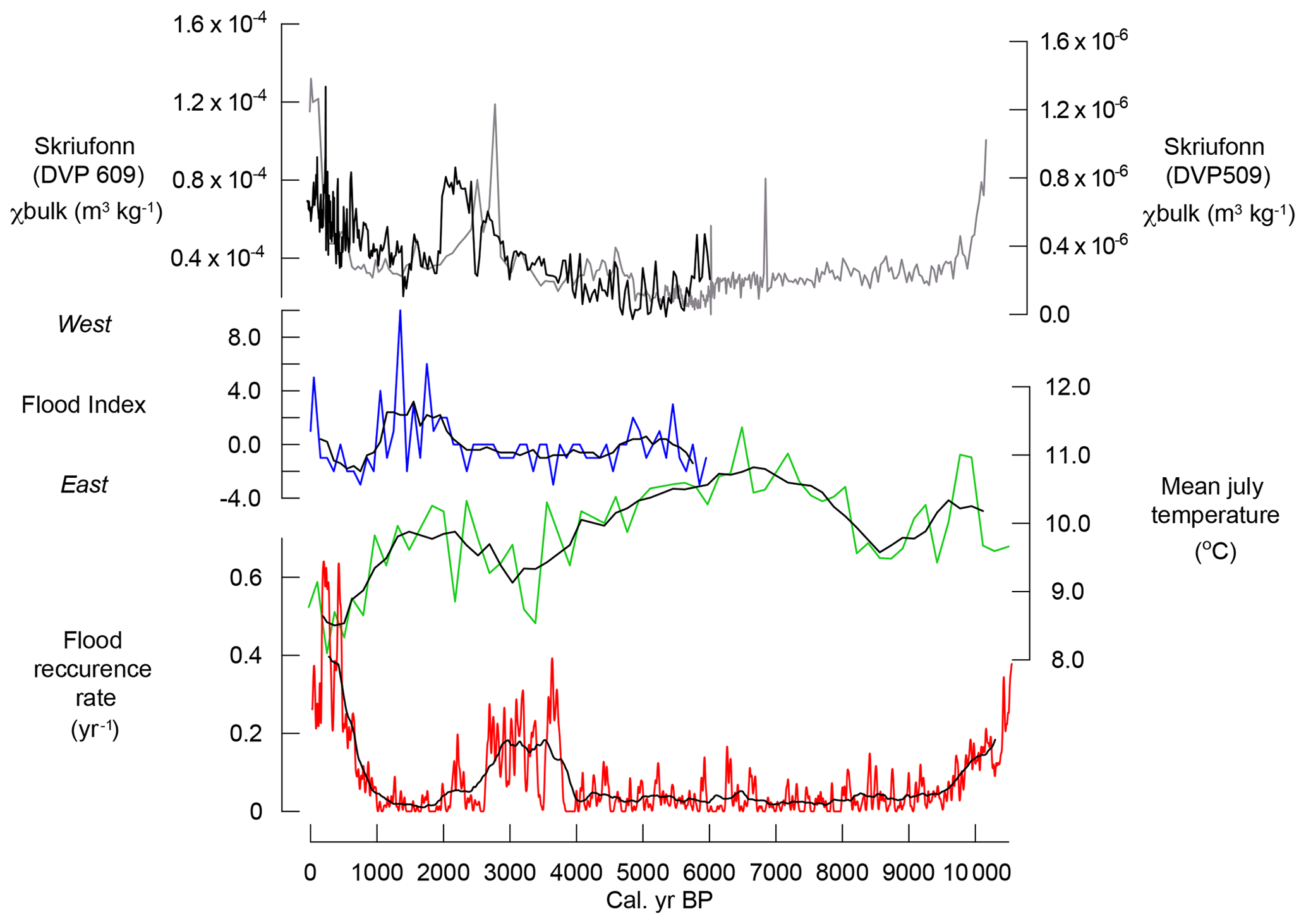
Figure 18Flood frequency in Glomma (red) with a 500-year running average, reconstructed summer temperature from Brurskardtjørni, southern Norway (Velle et al., 2010) (green) with a five-point running average, and flood index (blue) with a five-point running average (Støren et al., 2012) showing the relative distribution of the flood recurrence rate over southern Norway. Glacier activity at Skriufonn, Rondane, southern Norway (Kvisvik et al., 2015) (black and purple).
Another period with heightened flood activity occurred roughly between 4000 and 2000 years ago. The increase in flood frequency in Glomma during this period, and also during the LIA interval, coincides with a recorded decrease in summer temperature at Bruskardstjørni in eastern Jotunheimen (Velle et al., 2010) and increasing glacier growth in Rondane (Kvisvik et al., 2015), the mountainous source area of Glomma (Fig. 18). Multi-decadal periods are typically superimposed on centennial trends, as is the case for both these two flood-rich intervals. The near absence of floods prior to 4000 years ago is another recurring feature in all flood records from eastern Norway (e.g. Støren et al., 2016). Locally, it seems plausible that the effect of raising the 0-isotherm with 100–300 m altitude, the effect of a warmer summer season, will significantly change the potential storage of snow (Støren and Paasche, 2014).
The observed changes in flood frequency occurring during both the LIA and the first half of what sometimes is called the Neoglacial era (4000–2000 years ago) can thus, at least partially, be explained by the combined effect of the flood-generating processes (cf. Vormoor et al., 2016). The near absence of floods prior to the onset of the Neoglacial, when summer temperatures were ca. 1 ∘C higher than today (Velle et al., 2010), may be a valuable albeit imperfect analogue for the coming century. During this period the 200-year flood was around 30 % lower than today (Fig. 16).
In large catchments where snowmelt is the primary flood-generating process, it is suggested that we may see smaller flood sizes for eastern Norway according to Lawrence (2020). For small catchments, in western Norway, where rain-generated floods already dominate, floods are expected to increase. Cooler temperatures, especially in summer and spring, are likely to delay the melting of the snow cover – a scenario increasing the probability of a sudden warming simply because it occurs later in the season.
The increase in flood frequency commencing at ca. 4000 yr BP is a reoccurring feature not only in Europe, but also in parts of the USA (Paasche and Støren, 2014). This hints at a large-scale change in the climate system at the time, with implications for both atmospheric circulation patterns and temperature trends. This major climate shift recorded in Europe is noteworthy because the flood seasonality is different across such a large area for many reasons, including the varying altitudinal differences. In high-lying areas in Austria (north of the Alps, Swierczynski et al., 2013) and in the central Alps (Switzerland and northern Italy, Wirth et al., 2013), floods start to increase, as in eastern Norway, rapidly just after 4000 years ago and remain on average high until 2000 years ago. Studying the relative distribution of floods in Norway, Støren et al. (2012) suggest that the long-term trends in the floods are dependent on changes in the distribution of winter precipitation related to semi-permanent shifts in atmospheric circulation patterns and that an anomalously strong meridional component in the atmospheric circulation pattern is linked to floods in eastern Norway. Over the time period between the two flood-rich periods in Glomma (ca. 2000–1000 yr BP), Støren et al. (2012) recorded a westward shift in the flood frequency likely caused by reduced precipitation in the eastern areas (Fig. 18).
There are also potential catchment feedback mechanisms, not necessarily related to climate, that can both dampen and boost the flood patterns. Humans can potentially influence the landscape by forest clearing, which would alter sediment availability and runoff patterns as well as change the overall buffering capacity.
The flood-rich period occurring between 2500 and 4000 yr BP coincidences largely with the Bronze Age (2500–3700 BP), when settlements and farming expanded in Norway (Hjelle et al., 2018), but whether this early colonization impacted flood patterns remains an open question. Its worthwhile noticing that this interval with increased flooding is also recorded in other lake sediment records from southern Norway (Støren et al., 2010; Bøe et al., 2006) which were only marginally impacted by human activity, if at all (shown in Fig. 18), by farming. We therefore argue that the effect of land use cannot be the main explanation for the observed changes in flood frequency during this period. A similar conclusion was reached by Shubert et al. (2020), who show that logging and agricultural activities around the Mondsee, Austria, were low during flood-rich periods and that the flood record reflects climate variability rather than human activity in the catchment.
In more recent times, deforestation is a candidate that potentially could help explain the increase in flood frequency after 1600 CE. The mining industry that started in Norway in the late 16th century required a large amount of timber, which resulted in widespread deforestation in Glomma's upper catchment. This removal of woodland cover may have influenced the local erosion and sediment transport of the upstream Glomma catchment, but because this area represents only a fraction of the total catchment area, we think that these “excess sediments” would be diluted downstream. Another relevant point here is that the flat downstream gradient of the Glomma River potentially causes sediment deposition long before it reaches the bifurcation point at Kongsvinger. A final point is that the sediment source for the flood layers deposited in Flyginnsjøen is suggested to be mainly local, and the area around the lake and the location of the bifurcation events themselves were not subject to removal of woodland in this period. It is possible that the removal of woodland amplified the size (and frequency) of floods since forests, in most cases, reduce flood peaks. This, however, requires more regional and systematic vegetation change than that related to mining in the upper Glomma catchment to affect the 154 450 km2 large catchment. Some of these mechanisms discussed above could potentially help explain why Stor-Ofsen in 1789 is the largest local flood on record. As mentioned, this flood deposited the thickest sediment layer in the entire record from Flyginnsjøen. The anomalous sediment thickness is also recorded in lake sediment archives for other places in eastern Norway (see Bøe et al., 2006). Another amplifying process that can make floods become larger and also remobilize a larger amount of sediments, as is the case for Stor-Ofsen, was the large number of upstream landslides that took place at the time (Roald, 2013). In fact, the summer of 1789 was named “skriusommaren” (the landslide summer) in the historical material (Roald, 2013).
5.3 Flood quantile estimation by combining systematic, historical, and paleoflood data
The non-stationarity in flood frequency is a major challenge when estimating flood quantiles used for land planning and design of infrastructure given that one needs to predict how the flood frequency will evolve over the lifetime of the construction; e.g. for bridges it is 100 years (Koh et al., 2014). Milly et al. (2008) argued that “stationarity is dead” and that it is necessary to account for non-stationarity in order to avoid underestimation of risks based on design floods.
Conversely, Serinaldi and Kilsby (2015) posited that “stationarity is undead” because a stationary model is robust and can be a useful reference/benchmark. Accounting for uncertainty in a stationary model can be as important as including non-stationarity within a risk assessment framework. A non-stationary model introduces more parameters and, thereby, in most cases increases the estimation uncertainty. An additional challenge when applying a non-stationary model for design flood estimation is to project the flood frequency into the future.
The paleoflood data presented here suggest that the flood frequency is non-stationary and that there are indeed flood-rich and flood-poor periods (Fig. 13). Since design flood estimates are used for assessing average risk over the lifetime of a construction, it is desired that design flood estimates are stable over time and not sensitive to quasi-cyclic variations in flood sizes on annual to decadal timescales. It is, however, important to account for trends or shifts in flood frequency. Macdonald et al. (2014) show that on centennial timescales, the effect of cyclic variations in short systematic records can effectively be removed by a temporal extension of flood time series using historical information. Data from Flyginnsjøen and historical data reveal that a quasi-stationary period can be identified at centennial timescales but not on a sub-millennium timescale where major shifts in flood frequency are identified (Fig. 13).
In this study, we firstly used the stationarity assumption and evaluated several possible ways to combine the three data sources within a stationary framework. The results in Figs. 14 and 15 show that the design flood estimates are sensitive to how we combine the systematic, historical, and paleo flood data. We used 65 years of systematic data covering the period 1872–1936 CE for which we assume that the effect of river regulation is negligible. Adding the historical data from the flood stone covering the period from 1653 to 1871 CE substantially increased the estimates of the flood quantiles and slightly reduced the estimation uncertainty (Fig. 14).
The paleoflood time series provided here suggests that the flood frequency during the historical period is non-stationary where the 18th century was an extremely flood-rich period (Fig. 13) and that the 1789 CE flood was an exceptional flood during the 10 300 years covered by the sediment core. Based on this paleo information, we used historical data from the 19th century and added the 1789 CE flood by assuming it was the largest flood over a period of 10 300 years. This slightly reduced the flood quantile estimates as compared to using all historical information and substantially reduced the estimation uncertainty (Fig. 14). These results show that for the site at Elverum, we should be careful when including historical flood information from the flood-rich period in the 18th century.
As a next step, we added the paleoflood data representing 572 years (i.e. 1300–1871 CE). This resulted in negligible differences in flood quantile and uncertainty estimates (Fig. 15) indicating that the information content in the paleodata alone can be small. A possible explanation is the combination of the relatively low threshold (according to Fig. 15 it is around a 5-year flood) and that we only had information on the number of flood events. Both Macdonald et al. (2014) and Engeland et al. (2018) show that the information content is low when the threshold for historical floods is too low.
In a final step we used the flood rate from the sediment core as a key to explore non-stationarity of the design flood estimates, exemplified by the 200-year flood (Fig. 16). We could see important variation during the recent 6000 years. The 200-year flood was estimated to be around 23 % higher during the flood-rich periods in the 18th century and 20 % lower during the warmest period. The high values for the 200-year flood during the 18th century is confirmed by the historical data. This variation in design floods is, interestingly within the range seen in recent studies on climate change impacts on floods in Norway (Lawrence, 2020). For a future climate that is expected to be warmer, the design flood might be expected to decrease. Furthermore, this shows that the most interesting information we could get from the sediment core was the non-stationarity in floods.
In this study we have (i) compiled historical flood data from the existing literature, (ii) presented an analysis of the sediment core extracted from Lake Flyginnsjøen in Norway including results of XRF and CT scans plus MS measurements and used these data to estimate flood frequency over a period of 10 300 years, and (iii) combined flood data from systematic streamflow measurements, historical sources, and lacustrine sediment cores for estimating design floods and assessing non-stationarities in flood frequency at Elverum in the Glomma catchment located in eastern Norway. Our results show the following.
-
Based on detailed analysis of lake sediments that trap sediments whenever the Glomma River exceeds a local threshold, we could estimate flood frequency in a moving window of 50 years throughout the last 10 300 years.
-
The paleodata show that the flood frequency is non-stationary across timescales. Flood-rich periods has been identified, and these periods corresponds well to similar data in eastern Norway and also in the Alps such as the increase around 4000 years ago. The flood frequency can show significant non-stationarities within a flood-rich period. The most recent period with a high flood frequency was the 18th century, and the 1789 flood (Stor-Ofsen) is probably the largest flood during the entire Holocene.
-
The estimation of flood quantiles benefits from the use of historical and paleo data. The paleodata were in particular useful for evaluating the historical data. We identified that the 1789 flood was the largest one for the recent 10 300 years and that the 18th century was a flood-rich period as compared to the 20th and 19th centuries. Using the frequency of floods obtained from the paleoflood record resulted in minor changes in design flood estimates.
-
We could use the paleodata to explore non-stationarity in design flood estimates. During the coldest period in the 18th century, the design flood was up to 23 % higher than today, and down to 30 % lower in a warmer climate ca. 4000–6000 years ago.
This study has demonstrated the usefulness of paleoflood data, and we suggest that paleodata have a high potential for detecting links between climate dynamics and flood frequency. The data presented in this study could be used alone or in combination with paleoflood data from other locations in Norway and Europe to analyse the links between changes in climate and its variability and flood frequency.
Systematic flood data are available from the national hydrological database at the Norwegian Water Resources and Energy Directorate. The data from the scanning of the sediment cores are available upon request to the authors.
The study was designed and planned by AA, KE, IS, and ES. IS and ES carried out the lake coring and the field work. AA, IS, ØP, and ES all contributed the scanning and analysis of the sediment cores. AA, KE, and ES contributed to systematization of historical and systematic flood data and the flood frequency analysis. AA prepared Figs. 1 and 3. ES and ØP prepared Fig. 4. ES prepared Figs. 5, 9–11, and 18. KE prepared Figs. 2, 6–8, and 12–17. KE prepared the manuscript with contributions from all the co-authors.
The authors declare that they have no conflict of interest.
We would like to extend our thanks to Svein Olaf Dahl, Nils Roar Sæltun, and Chong-Yu Xu, who co-supervised the master projects of Ida Steffensen (Dept. of Geography, UiB) and Anna Aano (Dept. of Geoscience, UiO) that create the basis for this study, and Karoline Follestand and Martin Tvedt, who assisted in coring Lake Flyginnsjøen. This study became part of the Hordaflom project which is funded by RFF-Vest, Hordaland County. Øyvind Paasche is grateful to project ACER, funded by the Research Council of Norway. All core samples, apart from the dating, were measured at the Earth Surface Sediment Laboratory (EARTHLAB) at the Department of Earth Science, University of Bergen.
This research has been supported by the Research Council of Norway (grant nos. 812957 and 226171) and the RFF Vestlandet (grant no. 269682).
This paper was edited by Roger Moussa and reviewed by Daniel Schillereff and one anonymous referee.
Aano, A.: Flood frequency analyses based on streamflow time series, historical information and paleohydrological data, MS thesis, University of Oslo, Oslo, Norway, 2017.
Alfieri, L., Bisselink, B., Dottori, F., Naumann, G., de Roo, A., Salamon, P., Wyser, K. and Feyen, L.: Global projections of river flood risk in a warmer world, Earth's Future, 5, 171–182, https://doi.org/10.1002/2016EF000485, 2017.
Appleby, P. G.: Chronostratigraphic Techniques in Recent Sediments, in: Environmental Change Using Lake Sediments Volume 1: Basin Analysis, Coring, and Chronological Techniques, edited by: Last, W. M. and Smol, J. P., Springer, Dordrecht, the Netherlands, 171–203, https://doi.org/10.1007/0-306-47669-X_9, 2001.
Appleby, P. G. and Piliposian, G. T.: Radiometric Dating of Lake Sediment Cores from Flyginnsjøen and Vingersjøen, Southern Norway (provisional report), Environmental Radioactivity Research Centre, University of Liverpool, Liverpool, 2014.
Baker, V. R.: Paleohydrology and sedimentology of lake missoula flooding in Eastern Washington, Special Paper of the Geological Society of America 144, Geological Society of America, Boulder, Colorado, 1–73, https://doi.org/10.1130/SPE144-p1, 1973.
Baker, V. R.: Paleoflood hydrology and extraordinary flood events, J. Hydrol., 96, 79–99, https://doi.org/10.1016/0022-1694(87)90145-4, 1987.
Baker, V. R.: Paleoflood hydrology: Origin, progress, prospects, Geomorphology, 101, 1–13, https://doi.org/10.1016/j.geomorph.2008.05.016, 2008.
Benito, G. and O'Connor, J. E.: Quantitative paleoflood hydrology, in: Treatise on Geomorphology, vol. 9, Fluvial Geomorphology, edited by: Shroder, J. F. and Wohl, E., Academic Press, San Diego, 459–474, https://doi.org/10.1016/B978-0-12-374739-6.00250-5, 2013.
Benito, G. and Thorndycraft, V. R.: Palaeoflood hydrology and its role in applied hydrological sciences, J. Hydrol., 313, 3–15, https://doi.org/10.1016/j.jhydrol.2005.02.002, 2005.
Benito, G., Brázdil, R., Herget, J., and Machado, M. J.: Quantitative historical hydrology in Europe, Hydrol. Earth Syst. Sci., 19, 3517–3539, https://doi.org/10.5194/hess-19-3517-2015, 2015.
Benson, M. A.: Use of historical data in flood-frequency analysis, Eos Trans. Am. Geophys. Union, 31, 419–424, https://doi.org/10.1029/TR031i003p00419, 1950.
Blaauw, M. and Christeny, J. A.: Flexible paleoclimate age-depth models using an autoregressive gamma process, Bayesian Anal., 6, 457–474, https://doi.org/10.1214/11-BA618, 2011.
Blake, G. R. and Hartge, K. H.: Bulk Density, in: Methods of Soil Analysis: Part 1 – Physical and Mineralogical Methods, edited by: Klute, A., American Society of Agronomy – Soil Science Societey of America, Madison, 363–375, https://doi.org/10.2136/sssabookser5.1.2ed.c13, 1986.
Blöschl, G., Hall, J., Parajka, J., Perdigão, R. A. P., Merz, B., Arheimer, B., Aronica, G. T., Bilibashi, A., Bonacci, O., Borga, M., Čanjevac, I., Castellarin, A., Chirico, G. B., Claps, P., Fiala, K., Frolova, N., Gorbachova, L., Gül, A., Hannaford, J., Harrigan, S., Kireeva, M., Kiss, A., Kjeldsen, T. R., Kohnová, S., Koskela, J. J., Ledvinka, O., Macdonald, N., Mavrova-Guirguinova, M., Mediero, L., Merz, R., Molnar, P., Montanari, A., Murphy, C., Osuch, M., Ovcharuk, V., Radevski, I., Rogger, M., Salinas, J. L., Sauquet, E., Šraj, M., Szolgay, J., Viglione, A., Volpi, E., Wilson, D., Zaimi, K., and Živković, N.: Changing climate shifts timing of European floods, Science, 357, 588–590, https://doi.org/10.1126/science.aan2506, 2017.
Blöschl, G., Hall, J., Viglione, A., Perdigão, R. A. P., Parajka, J., Merz, B., Lun, D., Arheimer, B., Aronica, G. T., Bilibashi, A., Boháč, M., Bonacci, O., Borga, M., Čanjevac, I., Castellarin, A., Chirico, G. B., Claps, P., Frolova, N., Ganora, D., Gorbachova, L., Gül, A., Hannaford, J., Harrigan, S., Kireeva, M., Kiss, A., Kjeldsen, T. R., Kohnová, S., Koskela, J. J., Ledvinka, O., Macdonald, N., Mavrova-Guirguinova, M., Mediero, L., Merz, R., Molnar, P., Montanari, A., Murphy, C., Osuch, M., Ovcharuk, V., Radevski, I., Salinas, J. L., Sauquet, E., Šraj, M., Szolgay, J., Volpi, E., Wilson, D., Zaimi, K., and Živković, N.: Changing climate both increases and decreases European river floods, Nature, 573, 108–111, https://doi.org/10.1038/s41586-019-1495-6, 2019.
Bøe, A.-G., Dahl, S. O., Lie, Ø., and Nesje, A.: Holocene river floods in the upper Glomma catchment, southern Norway: a high-resolution multiproxy record from lacustrine sediments, Holocene, 16, 445–455, https://doi.org/10.1191/0959683606hl940rp, 2006.
Brázdil, R., Pfister, C., Wanner, H., von Storch, H., and Luterbacher, J.: Historical climatology in Europe – The state of the art, Climatic Change, 70, 363–430, https://doi.org/10.1007/s10584-005-5924-1, 2005.
Brázdil, R., Kundzewicz, Z. W., and Benito, G.: Historical hydrology for studying flood risk in Europe, Hydrolog. Sci. J., 51, 739–764, https://doi.org/10.1623/hysj.51.5.739, 2006a.
Brázdil, R., Kundzewicz, Z. W., and Benito, G.: Historical hydrology for studying flood risk in Europe, Hydrolog. Sci. J., 51, 739–764, https://doi.org/10.1623/hysj.51.5.739, 2006b.
Brázdil, R., Máčka, Z., Řezníčková, L., Soukalová, E., Dobrovolný, P., and Grygar, T. M.: Floods and floodplain changes of the River Morava, the Strážnické Pomoraví region (Czech Republic) over the past 130 years, Hydrolog. Sci. J., 56, 1166–1185, https://doi.org/10.1080/02626667.2011.608359, 2011.
Brázdil, R., Kundzewicz, Z. W., Benito, G., Demarée, G., Macdonald, N., and Roald, L. A.: Historical floods in europe in the past millennium, IAHS-AISH Publ., 10, 121–166, https://doi.org/10.1201/b12348-7, 2012.
Bretz, J. H.: Valley Deposits Immediately East of the Channeled Scabland of Washington. I, J. Geol., 37, 393–427, https://doi.org/10.1086/623636, 1929.
Coles, S. G. and Dixon, M. J.: Likelihood-Based Inference for Extreme Value Models, Extremes, 2, 5–23, https://doi.org/10.1023/A:1009905222644, 1999.
Cunnane, C. Unbiased plotting positions – a review – comments, J. Hydrol., 37, 205–222, https://doi.org/10.1016/0022-1694(78)90017-3, 1978.
Czymzik, M., Brauer, A., Dulski, P., Plessen, B., Naumann, R., von Grafenstein, U., and Scheffler, R.: Orbital and solar forcing of shifts in Mid- to Late Holocene flood intensity from varved sediments of pre-alpine Lake Ammersee (southern Germany), Quaternary Sci. Rev., 61, 96–110, https://doi.org/10.1016/j.quascirev.2012.11.010, 2013.
Dana, J. D.: The flood of the Connecticut River valley from the melting of the Quaternary glacier, Am. J. Sci., s3-23, 87–97, https://doi.org/10.2475/ajs.s3-23.134.87, 1882.
Dean Jr., W. E.: Determination of Carbonate and Organic Matter in Calcareous Sediments and Sedimentary Rocks by Loss on Ignition: Comparison With Other Methods, SEPM J. Sediment. Res., 44, 242–248, https://doi.org/10.1306/74d729d2-2b21-11d7-8648000102c1865d, 1974.
Debret, M., Chapron, E., Desmet, M., Rolland-Revel, M., Magand, O., Trentesaux, A., Bout-Roumazeille, V., Nomade, J., and Arnaud, F.: North western Alps Holocene paleohydrology recorded by flooding activity in Lake Le Bourget, France, Quaternary Sci. Rev., 29, 2185–2200, https://doi.org/10.1016/j.quascirev.2010.05.016, 2010.
Embrechts, P., Klüppelberg, C., and Mikosch, T.: Modelling Extremal Events, Springer, Berlin, Heidelberg, 1997.
Engeland, K., Wilson, D., Borsányi, P., Roald, L., and Holmqvist, E.: Use of historical data in flood frequency analysis: A case study for four catchments in Norway, Hydrol. Res., 49, 466–486, https://doi.org/10.2166/nh.2017.069, 2018.
Evin, G., Wilhelm, B., and Jenny, J. P.: Flood hazard assessment of the Rhône River revisited with reconstructed discharges from lake sediments, Global Planet. Chang, 172, 114–123, https://doi.org/10.1016/j.gloplacha.2018.09.010, 2019.
Finne-Grønn, S. H.: Elverum: en bygdebeskrivelse. 2: Bygdens almindelige historie, institutioner og embedsmænd, Cammenmeyers Boghandel, Oslo, available at: https://www.nb.no/items/0c92bf63bcd34a40d851ec9aed2d8f07?page=243&searchText=elverum en bygdebeskrivelse (last access: 5 March 2020), 1921.
Fisher, R. A. and Tippett, L. H. C.: Limiting forms of the frequency distribution of the largest or smallest member of a sample, Math. Proc. Cambridge Philos. Soc., 24, 180–190, https://doi.org/10.1017/S0305004100015681, 1928.
Follestad, K.: Reconstruction of floods in Glomma through the holosen – Effects of climate change on different flood regimes (Rekonstruksjon av flommer i Glomma gjennom holosen – Effekter av klimaendringer på ulike flomregimer – in Norwegian), MS thesis, University of Bergen, Bergen, available at: http://bora.uib.no/bitstream/handle/1956/9148/127896747.pdf (last access: 19 November 2020), 2014.
Gaál, L., Szolgay, J., Kohnová, S., Hlavčová, K., and Viglione, A.: Inclusion of historical information in flood frequency analysis using a Bayesian MCMC technique: a case study for the power dam Orlík, Czech Republic, Contrib. Geophys. Geod., 40, 121–147, https://doi.org/10.2478/v10126-010-0005-5, 2010.
Gilli, A., Anselmetti, F. S., Glur, L., and Wirth, S. B.: Lake Sediments as Archives of Recurrence Rates and Intensities of Past Flood Events, in: Dating Torrential Processes on Fans and Cones, vol. 47, edited by: Schneuwly-Bollschweiler, M., Stoffe, M., and Rudolf-Miklau, F., Springer, Dordrecht, the Netherlands, 225–242, https://doi.org/10.1007/978-94-007-4336-6_15, 2013.
Glaser, R., Riemann, D., Schönbein, J., Barriendos, M., Brázdil, R., Bertolin, C., Camuffo, D., Deutsch, M., Dobrovolný, P., van Engelen, A., Enzi, S., Halíčková, M., Koenig, S. J., Kotyza, O., Limanówka, D., Macková, J., Sghedoni, M., Martin, B., and Himmelsbach, I.: The variability of European floods since AD 1500, Climatic Change, 101, 235–256, https://doi.org/10.1007/s10584-010-9816-7, 2010.
GLB: Glommen og Laagens Grukseierforening 1918–43, Grøndahl & Søns Boktrykkeri, Oslo, 1947.
Gnedenko, B.: Sur La Distribution Limite Du Terme Maximum D'Une Serie Aleatoire, Ann. Math., 44, 423–453, https://doi.org/10.2307/1968974, 1943.
Grønlund, A., Njøs, A., and Kløve, B.: Endringer i landbrukets arealbruk i Glommas nedbørfelt, Oslo, available at: http://publikasjoner.nve.no/hydra/rapport/n02.pdf (last access: 5 March 2020), 1999.
Hall, J., Arheimer, B., Borga, M., Brázdil, R., Claps, P., Kiss, A., Kjeldsen, T. R., Kriaučiūnienė, J., Kundzewicz, Z. W., Lang, M., Llasat, M. C., Macdonald, N., McIntyre, N., Mediero, L., Merz, B., Merz, R., Molnar, P., Montanari, A., Neuhold, C., Parajka, J., Perdigão, R. a. P., Plavcová, L., Rogger, M., Salinas, J. L., Sauquet, E., Schär, C., Szolgay, J., Viglione, A., and Blöschl, G.: Understanding flood regime changes in Europe: a state-of-the-art assessment, Hydrol. Earth Syst. Sci., 18, 2735–2772, https://doi.org/10.5194/hess-18-2735-2014, 2014.
Hanssen-Bauer, I. Førland, E. J. Haddeland, I., Hisdal, H., Lawrence, D., Mayer, S., Nesje, A., Sandven, J. E. Ø., Sandø, A. B., and Sorteberg, A., and Ådlandsvik, B.: Climate in Norway 2100: a knowledge based for climate adaptation, NCCS Report 1/2017, The Norwegian Center for Climate Services, Oslo, Norway, 2017.
Hegge, K.: Glommas Bifurkasjon Ved Kongsvinger, Norsk Geografisk Tidsskrift, 22, 166–171, https://doi.org/10.1080/00291956808551859, 1968.
Hegge, K.: Letter to: The Norwegian Forest Museum (Elverum, Norway), Large floods in Glomma (Store flommer i Glomma – in Norwegian), The Norwegian Water Resources and Energy Directorate, Oslo, Norway, 2 pp., 4 September 1969.
Hirabayashi, Y., Mahendran, R., Koirala, S., Konoshima, L., Yamazaki, D., Watanabe, S., Kim, H., and Kanae, S.: Global flood risk under climate change, Nat. Clim. Change, 3, 816–821, https://doi.org/10.1038/nclimate1911, 2013.
Hirsch, R. M. and Stedinger, J. R.: Plotting positions for historical floods and their precision, Water Resour. Res., 23, 715–727, https://doi.org/10.1029/WR023i004p00715, 1987.
Hjelle, K. L., Halvorsen, L. S., Prøsch-Danielsen, L., Sugita, S., Paus, A., Kaland, P. E., Mehl, I. K., Overland, A., Danielsen, R., Høeg, H. I., and Midtbø, I.: Long-term changes in regional vegetation cover along the west coast of southern Norway: the importance of human impact, J. Veg. Sci., 29, 404–415, https://doi.org/10.1111/jvs.12626, 2018.
Høgaas, F. and Longva, O.: Mega deposits and erosive features related to the glacial lake Nedre Glomsjø outburst flood, southeastern Norway, Quaternary Sci. Rev., 151, 273–291, https://doi.org/10.1016/j.quascirev.2016.09.015, 2016.
IPCC: Managing the Risks of Extreme Events and Disasters to Advance Climate Change Adaptation – IPCC, edited by: Field, C. B., Barros, V., Stocker, T. F., Qin, D., Dokken, D. J., Ebi, K. L., Mastrandrea, M. D., Mach, K. J., Plattner, G.-K., Allen, S. K., Tignor, M., and Midgley, P. M., Cambridge University Press, available at: https://www.ipcc.ch/report/managing-the-risks-of-extreme-events-and-disasters-to- (last access: 4 March 2020), 2012.
Jacobeit, J., Glaser, R., Luterbacher, J., and Wanner, H.: Links between flood events in central Europe since AD 1500 and large-scale atmospheric circulation modes, Geophys. Res. Lett., 30, 2–5, https://doi.org/10.1029/2002GL016433, 2003.
Killingland, K. E. N.: Extreme floods in Grimsa, upper Glomma, Reconstruction of flood frequency through holocene and vulnerability analysis of today's river (Ekstremflommer i Grimsa, øvre Glommavassdraget Rekonstruksjon av flomfrekvens gjennom holosen og sårbarhetsanalyse av dagens elv, MS thesis, University of Bergen, Bergen, available at: http://bora.uib.no/bitstream/handle/1956/3543/63038069.pdf (last access: 19 November 2020), 2009.
Kjeldsen, T. R., Macdonald, N., Lang, M., Mediero, L., Albuquerque, T., Bogdanowicz, E., Brázdil, R., Castellarin, A., David, V., Fleig, A., Gül, G. O., Kriauciuniene, J., Kohnová, S., Merz, B., Nicholson, O., Roald, L. A., Salinas, J. L., Sarauskiene, D., Šraj, M., Strupczewski, W., Szolgay, J., Toumazis, A., Vanneuville, W., Veijalainen, N., and Wilson, D.: Documentary evidence of past floods in Europe and their utility in flood frequency estimation, J. Hydrol., 517, 963–973, https://doi.org/10.1016/j.jhydrol.2014.06.038, 2014.
Klæboe, H.: Glommas bifurkasjon ved kongsvinger, Norsk Geografisk Tidsskrift, 11, 266–275, https://doi.org/10.1080/00291954608551633, 1946.
Kochel, R. C. and Baker, V. R.: Paleoflood hydrology, Science, 215, 353–361, https://doi.org/10.1126/science.215.4531.353, 1982.
Koh, H. M., Park, W., and Choo, J. F.: Lifetime design of long-span bridges, Struct. Infrastruct. Eng., 10, 521–533, https://doi.org/10.1080/15732479.2013.769013, 2014.
Kundzewicz, Z. (Ed.): Changes in flood risk in Europe, International Association of Hydrological Sciences, SP10, Wallingford, UK, 2012.
Kvernmoen, G. T. and Kvernmoen, T.: Flomopptegnelser (1740–1839), in: Elverum – en bygdebeskrivelse – II – Bygdens almenne historie, S. H. Finne-Grønn, Oslo, 1921.
Kvisvik, B. C., Paasche, Ø., and Dahl, S. O.: Holocene cirque glacier activity in Rondane, southern Norway, Geomorphology, 246, 433–444, https://doi.org/10.1016/j.geomorph.2015.06.046, 2015.
Lawrence, D.: Uncertainty introduced by flood frequency analysis in projections for changes in flood magnitudes under a future climate in Norway, J. Hydrol.: Reg. Stud., 28, 100675, https://doi.org/10.1016/j.ejrh.2020.100675, 2020.
Lovdata: Dam Safety Regulation (Forskrift om sikkerhet ved vassdragsanlegg, in Norwegian), available at: https://lovdata.no/dokument/SF/forskrift/2009-12-18-1600?q=damsikkerhet (last access: 5 March 2020), 2010.
Macdonald, N. and Sangster, H.: High-magnitude flooding across Britain since AD 1750, Hydrol. Earth Syst. Sci., 21, 1631–1650, https://doi.org/10.5194/hess-21-1631-2017, 2017.
Macdonald, N., Kjeldsen, T. R., Prosdocimi, I., and Sangster, H.: Reassessing flood frequency for the Sussex Ouse, Lewes: the inclusion of historical flood information since AD 1650, Na. Hazards Earth Syst. Sci., 14, 2817–2828, https://doi.org/10.5194/nhess-14-2817-2014, 2014.
Martins, E. S. and Stedinger, J. R.: Generalized maximum-likelihood generalized extreme-value quantile estimators for hydrologic data, Water Resour. Res., 36, 737–744, https://doi.org/10.1029/1999WR900330, 2000.
Martins, E. S. and Stedinger, J. R.: Historical information in a generalized maximum likelihood framework with partial duration and annual maximum series, Water Resour. Res., 37, 2559–2567, https://doi.org/10.1029/2000WR000009, 2001.
Milly, P. C. D., Betancourt, J., Falkenmark, M., Hirsch, R. M., Kundzewicz, Z. W., Lettenmaier, D. P., and Stouffer, R. J.: Stationarity Is Dead: Whither Water Management?, Science, 319, 573–574, https://doi.org/10.1126/science.1151915, 2008.
Moberg, A., Sonechkin, D. M., Holmgren, K., Datsenko, M. H., and Karlén, W.: Highly variable Northern Hemisphere temperatures reconstructed from low- and high-resolution proxy data, Nature, 433, 613–617, https://doi.org/10.1038/nature03265, 2005.
Mudelsee, M., Börngen, M., Tetzlaff, G., and Grünewald, U.: Extreme floods in central Europe over the past 500 years: Role of cyclone pathway “Zugstrasse Vb”, J. Geophys. Res.-Atmos., 109, 1–21, https://doi.org/10.1029/2004JD005034, 2004.
Nesje, A.: A piston corer for lacustrine and marine sediments, Arct. Alp. Res., 24, 257–259, https://doi.org/10.2307/1551667, 1992.
Nesje, A., Dahl, S. O., Matthews, J. A., and Berrisford, M. S.: A ∼4500 yr record of river floods obtained from a sediment core in Lake Atnsjøen, eastern Norway, J. Paleolimnol., 25, 329–342, https://doi.org/10.1023/A:1011197507174, 2001.
NVE flood zone maps: NVE flood zone maps, available at: https://gis3.nve.no/link/?link=flomsone (last access: 23 May 2020), 2020.
Orvedal, K. and Peereboom, I. O.: Flood zone map Førde (Flaumsonekart Delprosjekt Førde – in Norwegian), NVE Report 61/2014, The Norwegian Water Resources and Energy Directorate, Oslo, Norway, available at: http://publikasjoner.nve.no/rapport/2014/rapport2014_61.pdf (last access: 18 November 2020), 2014.
Østmoe, A.: The Large flood of 1789: the weather system that led to the largest flood disaster in Norway (Stor-ofsen 1789: værsystemet som førte til den største flomkatastrofen i Norge – in Norwegian), Oversiktsregisteret, Ski, Norway, 1985
Otnes, J.: Old floodmarks at River Glomma (Gamle flommerker langs Glåma, Årbok for Glåmdalen 41, 6–26), Elverum Trykk, Elverum, 1982.
Paasche, Ø. and Støren, E. W. N.: How Does Climate Impact Floods? Closing the Knowledge Gap, Eos Trans. Am. Geophys. Union, 95, 253–254, https://doi.org/10.1002/2014EO280001, 2014.
Payrastre, O., Gaume, E., and Andrieu, H.: Usefulness of historical information for flood frequency analyses: Developments based on a case study, Water Resour. Res., 47, W08511, https://doi.org/10.1029/2010WR009812, 2011.
Pettersson, L.-E.: Flood estimation for the Glomma river upstream Vorma (Flomberegning for Glommavassdraget oppstrøms Vorma – in Norwegian), Oslo, available at: https://www.nve.no/ (last access: 5 March 2020), 2000.
Pettersson, L.-E.: Glomma's bifucation at Kongsvinger (Glommas bifurkasjon ved Kongsvinger – in Norwegian), Oslo, available at: https://www.nve.no/ (last access: 5 March 2020), 2001.
Prosdocimi, I.: German tanks and historical records: the estimation of the time coverage of ungauged extreme events, Stoch. Environ. Res. Risk A., 32, 607–622, https://doi.org/10.1007/s00477-017-1418-8, 2018.
Reimer, P. J., Bard, E., Bayliss, A., Beck, J. W., Blackwell, P. G., Ramsey, C. B., Buck, C. E., Cheng, H., Edwards, R. L., Friedrich, M., Grootes, P. M., Guilderson, T. P., Haflidason, H., Hajdas, I., Hatté, C., Heaton, T. J., Hoffmann, D. L., Hogg, A. G., Hughen, K. A., Kaiser, K. F., Kromer, B., Manning, S. W., Niu, M., Reimer, R. W., Richards, D. A., Scott, E. M., Southon, J. R., Staff, R. A., Turney, C. S. M., and van der Plicht, J.: IntCal13 and Marine13 Radiocarbon Age Calibration Curves 0–50,000 Years cal BP, Radiocarbon, 55, 1869–1887, https://doi.org/10.2458/azu_js_rc.55.16947, 2013.
Renard, B., Sun, X., and Lang, M.: Bayesian methods for nonstationary extreme value analysis, in: Extremes in a Changing Climate: Detection, Analysis and Uncertainty, Water Science and Technology Library, edited by: AghaKouchak, A., Easterling, D., Hsu, K., Schubert, S., and Sorooshian, S., Springer, the Netherlands, 39–95, https://doi.org/10.1007/978-94-007-4479-0_3, 2013.
Renberg, I. and Hansson, H.: The HTH sediment corer, J. Paleolimnol., 40, 655–659, https://doi.org/10.1007/s10933-007-9188-9, 2008.
Reusch, H.: Glomma's bend at Kongsvinger (Glommens bøining ved Kongsvinger), Norges Geografiske Selskab, Aarbog, 96–102, 1903.
Roald, L.: Floods in Norway (Flom i Norge – in Norwegian), Forlaget Tom& Tom, Oslo, 2013.
Schendel, T. and Thongwichian, R.: Considering historical flood events in flood frequency analysis: Is it worth the effort?, Adv. Water Resour., 105, 144–153, https://doi.org/10.1016/j.advwatres.2017.05.002, 2017.
Schillereff, D. N., Chiverrell, R. C., Macdonald, N., and Hooke, J. M.: Flood stratigraphies in lake sediments: A review, Earth-Sci. Rev., 135, 17–37, https://doi.org/10.1016/j.earscirev.2014.03.011, 2014.
Schubert, A., Lauterbach, S., Leipe, C., Scholz, V., Brauer, A., and Tarasov, P. E.: Anthropogenic and climate controls on vegetation changes between 1500 BCE and 500 CE reconstructed from a high-resolution pollen record from varved sediments of Lake Mondsee, Austria, Palaeogeogr. Palaeocl., 559, 109976, https://doi.org/10.1016/j.palaeo.2020.109976, 2020.
Serinaldi, F. and Kilsby, C. G.: Stationarity is undead: Uncertainty dominates the distribution of extremes, Adv. Water Resour., 77, 17–36, https://doi.org/10.1016/j.advwatres.2014.12.013, 2015.
Stedinger, J. R. and Cohn, T. A.: Flood Frequency Analysis With Historical and Paleoflood Information, Water Resour. Res., 22, 785–793, https://doi.org/10.1029/WR022i005p00785, 1986.
Steffensen, I. G.: Reconstruction of large floods in Glomma through the Holocene – possible links to natural climate variability and global atmospheric circulation (Rekonstruksjon av storflommer i Glomma gjennom holosen-mulige koblinger til naturlig klimavariabilitet og global atmosfaerisk sirkulasjon – in Norwegian), The University of Bergen, Bergen, 15 May 2014.
Støren, E. N. and Paasche, Ø.: Scandinavian floods: From past observations to future trends, Global Planet. Change, 113, 34–43, https://doi.org/10.1016/j.gloplacha.2013.12.002, 2014.
Støren, E. N., Dahl, S. O., Nesje, A., and Paasche, Ø.: Identifying the sedimentary imprint of high-frequency Holocene river floods in lake sediments: development and application of a new method, Quaternary Sci. Rev., 29, 3021–3033, https://doi.org/10.1016/j.quascirev.2010.06.038, 2010.
Støren, E. N., Kolstad, E. W., and Paasche, Ø.: Linking past flood frequencies in Norway to regional atmospheric circulation anomalies, J. Quaternary Sci., 27, 71–80, https://doi.org/10.1002/jqs.1520, 2012.
Støren, E. W. N., Paasche, Ø., Hirt, A. M., and Kumari, M.: Magnetic and geochemical signatures of flood layers in a lake system, Geochem. Geophy. Geosy., 17, 4236–4253, https://doi.org/10.1002/2016GC006540, 2016.
Swierczynski, T., Lauterbach, S., Dulski, P., Delgado, J., Merz, B., and Brauer, A.: Mid- to late Holocene flood frequency changes in the northeastern Alps as recorded in varved sediments of Lake Mondsee (Upper Austria), Quaternary Sci. Rev., 80, 78–90, https://doi.org/10.1016/j.quascirev.2013.08.018, 2013.
Tarr, R. S.: A hint with respect to the origin of terraces in glaciated regions, Am. J. Sci., s3-44, 59–61, https://doi.org/10.2475/ajs.s3-44.259.59, 1892.
TEK17: Building regulations (Byggtekninsk forskrift TEK17 – in Norwegian), available at: https://dibk.no/byggereglene/byggteknisk-forskrift-tek17/7/7-2/ (last access: 18 November 2020), 2018.
Velle, G., Bjune, A. E., Larsen, J., and Birks, H. J. B.: Holocene climate and environmental history of Brurskardstjørni, a lake in the catchment of Øvre Heimdalsvatn, south-central Norway, Hydrobiologia, 642, 13–34, https://doi.org/10.1007/s10750-010-0153-7, 2010.
Viglione, A.: nsRFA: Non-supervised Regional Frequency Analysis, R package version 0.7-11, available at: http://cran.r-project.org/package=nsRFA (last access: 18 November 2020), 2012.
Viglione, A., Merz, R., Salinas, J. L., and Blöschl, G.: Flood frequency hydrology: 3. A Bayesian analysis, Water Resour. Res., 49, 675–692, https://doi.org/10.1029/2011WR010782, 2013.
Vormoor, K., Lawrence, D., Schlichting, L., Wilson, D., and Wong, W. K.: Evidence for changes in the magnitude and frequency of observed rainfall vs. snowmelt driven floods in Norway, J. Hydrol., 538, 33–48, https://doi.org/10.1016/j.jhydrol.2016.03.066, 2016.
Walker, M., Johnsen, S., Rasmussen, S. O., Popp, T., Steffensen, J.-P., Gibbard, P., Hoek, W., Lowe, J., Andrews, J., Björck, S., Cwynar, L. C., Hughen, K., Kershaw, P., Kromer, B., Litt, T., Lowe, D. J., Nakagawa, T., Newnham, R., and Schwander, J.: Formal definition and dating of the GSSP (Global Stratotype Section and Point) for the base of the Holocene using the Greenland NGRIP ice core, and selected auxiliary records, J. Quaternary Sci., 24, 3–17, 2009.
Wellington, S. L. and Vinegar, H. J.: X-Ray Computerized Tompgraphy, J. Petrol. Technol., 39, 885–898, https://doi.org/10.2118/16983-PA, 1987.
Wilhelm, B., Ballesteros Canovas, J. A., Corella Aznar, J. P., Kämpf, L., Swierczynski, T., Stoffel, M., Støren, E., and Toonen, W.: Recent advances in paleoflood hydrology: From new archives to data compilation and analysis, Water Secur., 3, 1–8, https://doi.org/10.1016/j.wasec.2018.07.001, 2018.
Wirth, S. B., Glur, L., Gilli, A., and Anselmetti, F. S.: Holocene flood frequency across the Central Alps – solar forcing and evidence for variations in North Atlantic atmospheric circulation, Quaternary Sci. Rev., 80, 112–128, https://doi.org/10.1016/j.quascirev.2013.09.002, 2013.
The requested paper has a corresponding corrigendum published. Please read the corrigendum first before downloading the article.
- Article
(12137 KB) - Full-text XML