A skewed perspective of the Indian rainfall–El Niño–Southern Oscillation (ENSO) relationship

Wavelet coherence is a method that is commonly used in hydrology to extract scale-dependent, nonstationary relationships between time series. However, we show that the method cannot always determine why the time-domain correlation between two time series changes in time. We show that, even for stationary coherence, the time-domain correlation between two time series weakens if at least one of the time series has changing skewness. To overcome this drawback, a nonlinear coherence method is proposed to quantify the cross-correlation between nonlinear modes embedded in the time series. It is shown that nonlinear coherence and auto-bicoherence spectra can provide additional insight into changing time-domain correlations. The new method is applied to the El Niño–Southern Oscillation (ENSO) and all-India rainfall (AIR), which is intricately linked to hydrological processes across the Indian subcontinent. The nonlinear coherence analysis showed that the skewness of AIR is weakly correlated with that of two ENSO time series after the 1970s, indicating that increases in ENSO skewness after the 1970s at least partially contributed to the weakening ENSO–AIR relationship in recent decades. The implication of this result is that the intensity of skewed El Niño events is likely to overestimate India's drought severity, which was the case in the 1997 monsoon season, a time point when the nonlinear wavelet coherence between AIR and ENSO reached its lowest value in the 1871–2016 period. We determined that the association between the weakening ENSO–AIR relationship and ENSO nonlinearity could reflect the contribution of different nonlinear ENSO modes to ENSO diversity.

1 Introduction

The South Asian monsoon, which is the dominant precipitation source for the Indian subcontinent, has been a target for seasonal prediction for well over a century (Blanford, 1884). Despite this long heritage of research, skillful prediction remains a challenge, driving extensive and ongoing research on statistically and dynamically based prediction methods (e.g., REFS). It is difficult to overstate the importance of the South Asian monsoon to the well-being of citizens in India. Strong monsoon years have caused catastrophic flooding (Kale, 2012; Sanyal and Lu, 2005) and large landslides (Dortch et al., 2009), while weak monsoons have led to water shortages (Mishra et al., 2016) and crop losses (Parthasarathy et al., 1988; Prasanna, 2014) that resulted in significant food shortages in the past (Fagan, 2009). Thus, while the majority of monsoon forecast studies target the prediction of rainfall totals, the hydrological and agricultural impacts of monsoon variability provide the most pressing motivation for our work.

Much of the research on South Asian monsoon prediction has focused on the relationship between the El Niño–Southern Oscillation (ENSO; Walker and Bliss, 1932) and monsoon strength. During El Niño years, droughts are favored, while rainfall surpluses are favored during La Niña years (Shukla and Paolino, 1983; Kripalani and Kulkarni, 1997). However, there is no one-to-one relationship between ENSO and Indian rainfall. As a result, summer rainfall predictions based on ENSO have proven challenging. For example, the 1997–1998 El Niño event was extremely strong, yet climatological Indian monsoon conditions were observed (Shen and Kimoto, 1999; Slingo and Annamalai, 2000). It is therefore important to understand why certain El Niño events are not accompanied by monsoon failures.

There are a few reasons for the challenges faced when predicting Indian rainfall using ENSO. The first reason is that the relationship between ENSO and India's rainfall is nonstationary. As shown by Torrence and Webster (1999), the relationship between ENSO and India's rainfall cycles between periods of high and low coherence. Kumar et al. (1999) found that the relationship between Indian rainfall and ENSO weakened in the 1970s and hypothesized that a southward shift in Walker circulation anomalies associated with ENSO events and increased Eurasian spring and winter surface temperatures were responsible for the weakening relationship. Other works suggest that the changing ENSO–Indian rainfall relationship is the result of the modulating influence of tropical Atlantic sea surface temperatures (SSTs) and the Atlantic Multi-decadal Oscillation (AMO; Lu et al., 2006; Kucharski et al., 2007, 2009; Chen et al., 2010). In contrast, Kumar et al. (2006) and Fan et al. (2017) argued that the occurrence of different ENSO flavors (Johnson, 2013), such as the eastern Pacific and central Pacific types, could explain the ENSO–Indian rainfall relationship changes. Other investigators adopted another perspective to explain changes in the ENSO–Indian rainfall relationship and concluded that temporal undulations in the ENSO–Indian rainfall relationship are related to statistical undersampling and stochastic fluctuations (Gershunov et al., 2001; van Oldenborgh and Burgers, 2005; Delsole and Shukla, Cash et al., 2017). In a recent analysis, Yun and Timmermann (2018) showed that changes in the ENSO–Indian rainfall relationship are consistent with a stochastically perturbed ENSO signal and argued that changes in the ENSO–Indian monsoon relationship may not be related to external climate-forcing mechanisms.

The second reason for the ENSO-related prediction challenges is that ENSO itself is a nonstationary phenomenon. Using wavelet analysis, Kestin et al. (1998) found that the interannual variability of ENSO from 1930 to 1960 was dominated by a 4- to 7-year periodicity, whereas from 1960 to 1990 the interannual variability was also dominated by a 2- to 5-year periodicity. A wavelet power spectral analysis conducted by Torrence and Webster (1999) and Schulte (2016a) showed that ENSO signal energy in the 2- to 7-year band undulates throughout the historical period and increases after the 1960s (Schulte, 2016a). These changes in spectral characteristics are relevant to Indian monsoon prediction because differing spectral characteristics among predictors (e.g., ENSO) and predictands (e.g., Indian rainfall) can negatively impact the predictive skill of statistical models (Jiang et al., 2020). Using a wavelet-based variance transformation method, Jiang et al. (2020) demonstrated that accounting for differences in spectral characteristics can improve prognostic skill. That study suggests that Indian monsoon prediction could be improved by using wavelet-based methods instead of time-domain correlation and regression methods.

The nonlinear characteristics (e.g., skewness) of ENSO are also nonstationary and undergo interdecadal changes (Wu and Hsieh, 2003). Numerous studies have reported an ENSO regime shift in the 1970s in which ENSO began to evolve more nonlinearly than in previous decades (An, 2004, 2009; An and Jin, 2004). It is a curious fact that the ENSO regime shift in the 1970s coincided with the weakening ENSO–Indian rainfall relationship, as documented by Kumar et al. (1999). This observation creates a question that begs to be answered, namely whether nonlinear ENSO regime changes are related to changes in the ENSO–Indian rainfall relationship.

Various mechanisms have been proposed to explain the cause of ENSO skewness. Kang and Kug (2002) suggested that the asymmetry between the magnitude of El Niño and La Niña events is related to the relative westward displacement of zonal wind stress anomalies during La Niña events compared to El Niño events. Jin et al. (2003) and An and Jin (2004) found that ENSO asymmetry is related to nonlinear dynamical heating (NDH), where the magnitude of NDH is related to the propagation characteristics of ENSO. As shown by An and Jin (2004), NDH during strong El Niño events like the 1982–1983 and 1997–1998 events tends to be stronger than during weak El Niño events because SST anomalies tend to propagate eastward. Since the late 1970s there has been a propensity for eastward propagation characteristics of ENSO (Santoso et al., 2013), contrasting with the time period before the 1970s that consisted of the relatively weak El Niño events of 1957–1958 and 1972–1973 (An and Jin, 2004; An, 2009). More recently, Su et al. (2010) showed that vertical temperature advection may have an opposing effect on ENSO asymmetry, and that the asymmetry in the extreme eastern equatorial Pacific is related to meridional ocean temperature advection.

Previous investigators have used different metrics to quantify ENSO asymmetry. To measure the nonlinear character of ENSO, An and Jin (2004) used time-domain metrics, such as skewness and maximum potential intensity (MPI), to quantify the skewness of SST anomalies and the skewness of individual ENSO events, respectively. An (2004) applied a principal component analysis (PCA) to a 21-year moving window of tropical Pacific SST skewness and found that the first PCA mode is characterized by positive skewness across the eastern equatorial Pacific and negative skewness across the central equatorial Pacific. This pattern means that interdecadal changes in the nonlinearity of ENSO are associated with positively skewed SST anomalies across the eastern equatorial Pacific, implying that El Niño events are stronger than La Niña events. While the methods implemented in the aforementioned studies provided important insights, they cannot reveal the frequency modes of ENSO that are contributing to the skewness.

Recognizing the limitations of time-domain approaches, Timmermann (2003) conducted a bispectral analysis of the Niño 3 anomaly time series, where a peak (f₁; f₂) in the bispectrum means there is statistical phase dependence among oscillators with frequencies of f₁ and f₂ and f₁+f₂. That bispectral analysis revealed statistically significant bispectral power at several frequency pairs, including (0.038, 0.038), (0.028, 0.028), (0.0225, 0.0225), (0.0045, 0.032), and (0.0045, 0.045) [months⁻¹]. The peaks (0.0045, 0.032) and (0.0045, 0.045) [months⁻¹] were identified with the nonlinear interactions among the 18- and 2-year variability. Although the analysis provided new insights, the Fourier-based analysis could not reveal how the nonlinear nature of ENSO changed with time, which is an important property to capture given how the nonlinear characteristics of ENSO are nonstationary (Santoso et al., 2013). Much like the cross-wavelet power (Maraun and Kurths, 2004) and time-domain covariance, bispectral power is not a bounded quantity, and so high bispectral power does not always mean strong phase dependence.

In this study, the deficiencies associated with the abovementioned techniques are addressed using higher-order wavelet analysis, which allows for the quantification of frequency-dependent and nonstationary nonlinearities in time series (Van Milligen et al., 1995; Elsayed, 2006; Schulte, 2016b). More specifically, the objectives of the paper are the following: (1) to quantify the nonlinearity of ENSO using higher-order wavelet analysis together with recently developed statistical tests, (2) to determine if different nonlinear modes of ENSO are associated with distinct SST patterns, and (3) to develop nonlinear wavelet coherence methods to test the hypothesis that the breakdown of the ENSO–Indian rainfall relationship in recent decades is related to the shift of ENSO from a linear regime to a nonlinear one. The paper is organized as follows: in Sect. 2, the data used are described. Section 3 includes the description of the implemented methodologies. Results are presented in Sect. 4, and concluding remarks are provided in Sect. 5.

2 Data

The variability in India rainfall from 1871 to 2016 was analyzed using the all-India rainfall (AIR; Parthasarathy et al., 1994) time series, which was created by averaging representative rain gauges at various locations across India. The full monsoon season (June–September) and the late monsoon (August–September) season were used to identify possible within-season variations in the ENSO–all-India rainfall (ENSO–AIR) relationships. To remove the influence of the annual cycle, AIR time series were converted into anomaly time series by subtracting the 1871–2016 long-term mean for each month from the individual monthly values. The AIR anomaly (hereafter AIR) time series were subsequently standardized by dividing them by their 1871–2016 standard deviations. Because wavelet analysis focuses on specific frequency components that are not impacted by long-term time-domain trends, no detrending of the data was performed.

The monthly data for the Niño 1 and 2, Niño 3, Niño 3.4, and Niño 4 indices (available at: https://www.psl.noaa.gov/gcos_wgsp/Timeseries/, last access: 15 March 2019) from 1871 to 2016 were used to understand how the nonlinear characteristics of SSTs varied from one ENSO region to another. The Niño 1+2 index is the average SST in the region, with latitudinal boundaries of 0^∘ and 10^∘ S and longitudinal boundaries of 90 and 80^∘ W. The Niño 3 index is the average SST in the region, with latitudinal boundaries of 5^∘ N and 5^∘ S and longitudinal boundaries of 150 and 90^∘ W. Variations in SSTs further west were described using the Niño 3.4 and Niño 4 indices, where the Niño 3.4 index is defined as the average SST in the region bounded by 5^∘ N and 5^∘ S and 170 and 120^∘ W. The Niño 4 index is defined as average SSTs in the region bounded by 5^∘ N and 5^∘ S and 160^∘ E and 150^∘ W. The seasonal cycle was removed from these time series in the same way as it was removed from the AIR time series.

The monthly SST data from 1871 to 2016 were based on the Hadley Centre Global Sea Ice and Sea Surface Temperature (HadISST1; Rayner et al., 2003). The data at each grid point were converted to monthly anomalies in the same way as they were computed for the ENSO and AIR time series.

3 Methods

3.1 Wavelet analysis

To better diagnose the changes in time series statistics associated with AIR and ENSO, we adopted a wavelet analysis. For a time series, X, comprising data points $x_{\mathrm{1}},x_{\mathrm{2}},\mathrm{\dots },x_N$, the continuous wavelet transform is given by the following:

$$\begin{array}{}\text{(1)}& W_n\left(s\right)=\sqrt{{\displaystyle \frac{\mathit{\delta }t}{s}}}{\sum }_{n^{\prime =\mathrm{1}}}^N{x}_{n^{\prime }}{\mathit{\psi }}_{\mathrm{0}}\left[\left(n^{\prime }-n\right){\displaystyle \frac{\mathit{\delta }t}{s}}\right],\end{array}$$

where s is the wavelet scale, ψ₀ is an analyzing wavelet, δt is a time step (1 month in this study), and n is time. The sample wavelet power spectrum ${\left|W_n\left(s\right)\right|}^{\mathrm{2}}$ measured the energy content of a signal at time n and scale s. The commonly used Morlet wavelet, with angular frequency ω=6, was used throughout this paper because it balances time and frequency localization, and because it is commonly used in hydrological and climate studies (Schaefli et al., 2007; Zhang et al., 2007; Holman et al., 2011; Carey et al., 2013). The readers are referred to Torrence and Compo (1998) and Grinsted et al. (2004) for more details about wavelet analysis.

Linear wavelet coherence (Table 1) was used to quantify the linear relationship between two time series as a function of frequency and time. The linear wavelet coherence between two time series X and Y is given by the following:

$$\begin{array}{}\text{(2)}& R_n^{\mathrm{2}}\left(s\right)={\displaystyle \frac{{\left|S{s}^{-\mathrm{1}}{W}_n^{\mathrm{XY}}\left(s\right)\right|}^{\mathrm{2}}}{S\left(s^{-\mathrm{1}}{\left|W_n^X\left(s\right)\right|}^{\mathrm{2}}\right)S\left(s^{-\mathrm{1}}{\left|W_n^Y\left(s\right)\right|}^{\mathrm{2}}\right)}},\end{array}$$

where S is a smoothing operator (Grinsted et al., 2004) and $W_n^{\mathrm{XY}}\left(s\right)$ is the cross-wavelet power spectrum. Two time series are perfectly coherent ($R_n^{\mathrm{2}}\left(s\right)=\mathrm{1}$) at s if ${\mathit{\varphi }}_n^X\left(s\right)-{\mathit{\varphi }}_n^Y\left(s\right)=c$ over a sufficiently long time interval, where c is a constant, ${\mathit{\varphi }}_n^X\left(s\right)$ is the phase associated with X, and ${\mathit{\varphi }}_n^Y\left(s\right)$ is the wavelet phase associated with Y.

Table 1 Wavelet quantities and the relationships they measure.

In the context of the Indian monsoon, strong coherence between rainfall and a climate pattern (e.g., ENSO) at a scale s indicates shared temporal characteristics between a climate pattern and rainfall. Because the theory supports a causal link between ENSO and monsoon variability through changes in the Walker circulation (Ropelewski and Halpert, 1987), strong coherence means that when ENSO is in a warm (cool) phase at the scale s, negative (positive) rainfall anomalies are preferred. Thus, a periodic climate forcing could create periodicities in an otherwise noisy rainfall time series.

3.2 Higher-order wavelet analysis

Although the wavelet power spectrum is useful for quantifying the signal energy at a scale s and time n, it cannot determine if there is a nonlinear relationship among different frequency components. In fact, the power spectrum can only fully describe time series in frequency space in the case of linear systems in which the output is proportional to the input (King, 1996). As ENSO is nonlinear, we adopted higher-order wavelet methods to address the deficiencies in traditional wavelet methods. The type of nonlinearities considered in this study were quadratic nonlinearities in which the scales s₁, s₂, and s₃ satisfied the sum rule as follows:

$$\begin{array}{}\text{(3)}& {\displaystyle \frac{\mathrm{1}}{s_{\mathrm{3}}}}={\displaystyle \frac{\mathrm{1}}{s_{\mathrm{1}}}}+{\displaystyle \frac{\mathrm{1}}{s_{\mathrm{2}}}},\end{array}$$

and the wavelet phases satisfied the following:

$$\begin{array}{}\text{(4)}& {\mathit{\varphi }}_n\left(s_{\mathrm{3}}\right)={\mathit{\varphi }}_n\left(s_{\mathrm{1}}\right)+{\mathit{\varphi }}_n\left(s_{\mathrm{2}}\right).\end{array}$$

These types of nonlinearities arise, for example, when a sinusoid is squared, in which case a harmonic is produced. More generally, quadratic nonlinearities induce time series skewness, which was computed in this study using the following:

$$\begin{array}{}\text{(5)}& \text{skewness}={\displaystyle \frac{\frac{\mathrm{1}}{N}{\sum }_{i=\mathrm{1}}^N{\left(x_i-\overline{x}\right)}^{\mathrm{3}}}{\mathrm{SD}}},\end{array}$$

where SD in the standard deviation of the time series, and $\overline{x}$ is the mean of the time series. Positive (negative) skewness meant that the right (left) tail of the time series distribution is longer than the left (right). In other words, positive (negative) skewness meant that there was a tendency for positive (negative) time series events (i.e., anomalies) to be more intense than negative (positive) ones.

In this paper, quadratic nonlinearities giving rise to time series skewness were quantified using local and global wavelet-based auto-bicoherence methods (Schulte, 2016b). Global auto-bicoherence (Table 1) was computed as follows:

$$\begin{array}{}\text{(6)}& \begin{array}{rl}& {\mathrm{bi}}_{\mathrm{global}}^X\left(s_{\mathrm{1}},s_{\mathrm{2}}\right)=\\ & {\displaystyle \frac{{\left|B_{\mathrm{global}}^X\left(s_{\mathrm{1}},s_{\mathrm{2}}\right)\right|}^{\mathrm{2}}}{\left({\sum }_{n=\mathrm{1}}^N{\left|W_n^X\left(s_{\mathrm{1}}\right)W_n^X\left(s_{\mathrm{2}}\right)\right|}^{\mathrm{2}}\right)\left({\sum }_{n=\mathrm{1}}^N{\left|W_n^X\left(s_{\mathrm{3}}\right)\right|}^{\mathrm{2}}\right)}},\end{array}\end{array}$$

where

$$\begin{array}{}\text{(7)}& B_{\mathrm{global}}^X\left(s_{\mathrm{1}},s_{\mathrm{2}}\right)={\sum }_{n=\mathrm{1}}^N{\widehat{W}}_n^X\left(s_{\mathrm{3}}\right)W_n^X\left(s_{\mathrm{1}}\right)W_n^X\left(s_{\mathrm{2}}\right)\end{array}$$

is the global bispectrum, and the hat denotes the complex conjugate. Identical to wavelet coherence, auto-bicoherence is bounded by 0 and 1, with a value of 1 indicating the strongest possible phase coupling among the phases ϕ_n(s₃), ϕ_n(s₂), and ϕ_n(s₁), such that sum rules of Eqs. (3–4) are satisfied. A peak in the auto-coherence spectrum at (s₁, s₂) indicated that there was quadratic-phase coupling among oscillatory modes that was contributing to time series skewness. It is important to note that the auto-bicoherence method cannot detect other types of nonlinearities such as cubic nonlinearities, whose detection would require trispectra (Collis et al., 1998).

To determine if the strength of the quadratic-phase coupling was a function of time, the local auto-bicoherence spectrum (Schulte, 2016b) given by the following:

$$\begin{array}{}\text{(8)}& \begin{array}{rl}& {\mathrm{bi}}_n^X\left(s_{\mathrm{1}},s_{\mathrm{1}}\right)=\\ & {\displaystyle \frac{{\left|S{s}_{\mathrm{1}}^{-\mathrm{1}}{B}_n^X\left(s_{\mathrm{1}},s_{\mathrm{1}}\right)\right|}^{\mathrm{2}}}{S\left(s_{\mathrm{1}}^{-\mathrm{1}}{\left|W_n^X\left(s_{\mathrm{1}}\right)W_n^X\left(s_{\mathrm{1}}\right)\right|}^{\mathrm{2}}\right)S\left(s_{\mathrm{1}}^{-\mathrm{1}}{\left|W_n^X\left(\frac{s_{\mathrm{1}}}{\mathrm{2}}\right)\right|}^{\mathrm{2}}\right)}}\end{array}\end{array}$$

was computed, where $B_n^X\left(s_{\mathrm{1}},s_{\mathrm{1}}\right)$ is the local bispectrum, given as follows:

$$\begin{array}{}\text{(9)}& B_n^X\left(s_{\mathrm{1}},s_{\mathrm{1}}\right)={\widehat{W}}_n^X\left(s_{\mathrm{3}}\right)W_n^X\left(s_{\mathrm{1}}\right)W_n^X\left(s_{\mathrm{1}}\right)\end{array}$$

and $s_{\mathrm{3}}=s_{\mathrm{1}}/\mathrm{2}$. In this special case, the local auto-bicoherence spectrum revealed the time evolution of the auto-bicoherence estimates located along the diagonal slices of the global auto-bicoherence spectra. Local biphase is as follows:

$$\begin{array}{}\text{(10)}& {\mathit{\psi }}_n(s_{\mathrm{1}},s_{\mathrm{1}})={\mathit{\varphi }}_n\left(s_{\mathrm{1}}\right)+{\mathit{\varphi }}_n\left(s_{\mathrm{1}}\right)-{\mathit{\varphi }}_n\left(s_{\mathrm{3}}\right)\end{array}$$

and was used to measure the skewness and asymmetries of waveforms. A biphase of 0^∘ meant that the relationship among the scale components produced positive skewness with respect to a horizonal axis so that positive deviations from the mean are larger than negative deviations from the mean (King, 1996; Maccarone, 2013; Schulte, 2016b). On the other hand, a biphase of 180^∘ indicated negative skewness with respect to the mean. Biphases near −90^∘ or 90^∘ indicated that a time series rose (fell) more quickly than it fell (rose).

To be consistent with the wavelet power and coherence analyses, results for the higher-order wavelet analysis were casted in terms of the Fourier period rather than wavelet scale. The Fourier period corresponding to s_i was denoted by p_i, where the Fourier period is obtained by multiplying s_i by 1.03 for the Morlet wavelet (Torrence and Compo, 1998). Thus, the local diagonal slice of the auto-bicoherence spectra were plotted using the Fourier period p₁ corresponding to s₁ as the vertical axis and time as the horizonal axis.

3.3 Statistical hypothesis testing

The statistical significance of all wavelet spectra was evaluated using the cumulative area-wise test (Schulte, 2016a, 2019a) to account for the simultaneous testing of multiple hypotheses (Maraun and Kurths, 2004; Maraun et al., 2007). This test evaluated the statistical significance of points in the wavelet domain based on the area of contiguous regions of point-wise significance (i.e., patches) to which they belong, so a larger area implies a greater statistical significance. Given that the patch area can change as the point-wise significance changes, the cumulative area-wise test was used to evaluate significance based on the patch area averaged across a set of point-wise significance levels (Schulte, 2019a). The test was applied at the 5 % cumulative area-wise significance level, using point-wise significance levels ranging from 0.02 to 0.18, because this choice of point-wise significance levels was shown to result in the cumulative area-wise test outperforming the point-wise test in terms of true positive detection for moderate to high signal-to-noise ratios, even though the cumulative area-wise test is more stringent. The test was performed using the Advanced Biwavelet Wavelet R software package (available at: http://justinschulte.com/wavelets/advbiwavelet.html, last access: 20 July 2020). Technical details of the testing procedure can be found in Schulte (2019a) and Appendix A.

To assess the statistical significance of the global auto-bicoherence estimates, a modified version of the cumulative area-wise test was applied. In the modified version of the cumulative area-wise test, the normalized area of patches was computed by dividing the patch area by the product $\widehat{s_{\mathrm{1}}}\widehat{s_{\mathrm{2}}}$, where $\widehat{s_{\mathrm{1}}}$ is the mean first coordinate of the patch, and $\widehat{s_{\mathrm{2}}}$ is the mean second coordinate. The reason for this modified normalized area is that dividing area by, say, ${\widehat{s_{\mathrm{1}}}}^{\mathrm{2}}$ retained the correlation between the normalized area and s₂. The test was applied using the same point-wise significance levels that were used to assess the statistical significance of wavelet power and coherence.

3.4 Higher-order coherence

Although wavelet coherence spectra can provide information regarding how the relationship between two climate variables changes at a scale s, it cannot completely explain why the time-domain correlation between the climate variables temporally fluctuates. The reason is that linear wavelet coherence only examines how well the variance of one time series corresponds to the variance of another at a scale s (Table 1) because linear coherence is determined by the wavelet power spectra of the time series. However, for two time series to be perfectly correlated in the time domain, higher skewness of one time series must also correspond to higher skewness of the other time series.

Recognizing the skewness associated with two time series was correlated in frequency space using the following:

$$\begin{array}{}\text{(11)}& \begin{array}{rl}& {\mathrm{Bi}}_n^{\mathrm{2}}(s_{\mathrm{1}},s_{\mathrm{2}})=\\ & {\displaystyle \frac{{\left|S{s}_{\mathrm{smooth}}^{-\mathrm{1}}{B}_n^{\mathrm{XY}}(s_{\mathrm{1}},s_{\mathrm{2}})\right|}^{\mathrm{2}}}{S\left(s_{\mathrm{smooth}}^{-\mathrm{1}}{\left|B_n^X\left(s_{\mathrm{1}},s_{\mathrm{2}}\right)\right|}^{\mathrm{2}}\right)S\left(s_{\mathrm{smooth}}^{-\mathrm{1}}{\left|B_n^Y\left(s_{\mathrm{1}},s_{\mathrm{2}}\right)\right|}^{\mathrm{2}}\right)}},\end{array}\end{array}$$

which was referred to as third-order coherence (nonlinear coherence, hereafter; the readers are referred to Appendix B for a more general definition of higher-order coherence). In Eq. (11), s_smooth is one of the three scales, and $B_n^{\mathrm{XY}}(s_{\mathrm{1}},s_{\mathrm{2}})$ is the third-order cross-wavelet power spectrum, which is the product of the bispectrum of X and the conjugate of the bispectrum of Y, the higher-order analog of the cross-wavelet power spectrum. The word cross-bispectrum was not used to avoid confusion with cross-bicoherence analysis (Van Milligen,1995). Like wavelet coherence, the nonlinear coherence is bounded by 0 and 1, with a value of 1 indicating that the bispectra of X and Y at (s₁, s₂) are perfectly and linearly correlated. The statistical significance of nonlinear coherence was assessed using the cumulative area-wise test in the same way as it was used to assess the statistical significance of linear wavelet coherence.

Higher-order wavelet analysis can also be interpreted in terms of linear and nonlinear modes. A linear mode ${\mathit{\gamma }}_{s_i}^X$ is the signal component of X at the scale s_i obtained by setting all wavelet coefficients to zero, except those at s_i, and taking the inverse wavelet transform of the result. Because linear modes are only composed of a single frequency component, the local cross-correlation (coherence) between ${\mathit{\gamma }}_{s_i}^X$ and ${\mathit{\gamma }}_{s_i}^Y$ is only impacted by the variances in X and Y at s_i. On the other hand, nonlinear coherence measures the local cross-correlation between the skewness of ${\mathit{\gamma }}_{s_{\mathrm{1}}}^X+{\mathit{\gamma }}_{s_{\mathrm{2}}}^X+{\mathit{\gamma }}_{s_{\mathrm{3}}}^X$ and ${\mathit{\gamma }}_{s_{\mathrm{1}}}^Y+{\mathit{\gamma }}_{s_{\mathrm{2}}}^Y+{\mathit{\gamma }}_{s_{\mathrm{3}}}^Y$ or between ${\mathit{\gamma }}_{s_{\mathrm{1}}}^X+{\mathit{\gamma }}_{s_{\mathrm{1}}/\mathrm{2}}^X$ and ${\mathit{\gamma }}_{s_{\mathrm{1}}}^Y+{\mathit{\gamma }}_{s_{\mathrm{1}}/\mathrm{2}}^Y$ in the case that s₁=s₂.

To better understand nonlinear coherence, we supposed that, in the following:

$$\begin{array}{}\text{(12)}& {\displaystyle }{\mathit{\varphi }}_n^X\left(s_{\mathrm{1}}\right)-{\mathit{\varphi }}_n^Y\left(s_{\mathrm{1}}\right)={\mathrm{c}}_{\mathrm{1}}\text{(13)}& {\displaystyle }{\mathit{\varphi }}_n^X\left(s_{\mathrm{2}}\right)-{\mathit{\varphi }}_n^Y\left(s_{\mathrm{2}}\right)={\mathrm{c}}_{\mathrm{2}}\text{(14)}& {\displaystyle }{\mathit{\varphi }}_n^X\left(s_{\mathrm{3}}\right)-{\mathit{\varphi }}_n^Y\left(s_{\mathrm{3}}\right)={\mathrm{c}}_{\mathrm{3}}\end{array}$$

was applied for constants c₁, c₂, and c₃. Adding Eqs. (12) and (13) and subtracting Eq. (14) from the result produced the equality, as follows:

$$\begin{array}{}\text{(15)}& \begin{array}{rl}& {\mathit{\varphi }}_n^X\left(s_{\mathrm{1}}\right)+{\mathit{\varphi }}_n^X\left(s_{\mathrm{2}}\right)-{\mathit{\varphi }}_n^X\left(s_{\mathrm{3}}\right)-({\mathit{\varphi }}_n^Y\left(s_{\mathrm{1}}\right)+{\mathit{\varphi }}_n^Y\left(s_{\mathrm{2}}\right)\\ & -{\mathit{\varphi }}_n^Y\left(s_{\mathrm{3}}\right))={\mathit{\psi }}_n^X\left(s_{\mathrm{1}},s_{\mathrm{2}}\right)-{\mathit{\psi }}_n^Y\left(s_{\mathrm{1}},s_{\mathrm{2}}\right)=\\ & {\mathit{\psi }}_n^{\mathrm{bi}}\left(s_{\mathrm{1}},s_{\mathrm{2}}\right)=K,\end{array}\end{array}$$

for some constant $\mathrm{K}={\mathrm{c}}_{\mathrm{1}}+{\mathrm{c}}_{\mathrm{2}}-{\mathrm{c}}_{\mathrm{3}}.$ Thus, if X was found to be perfectly nonlinearly coherent with Y,then Xand Ywere perfectly coherent at the three scales participating in the quadratic-phase coupling. Even if the coherence was perfect at two scales, the relative biphase ${\mathit{\psi }}_n^{\mathrm{bi}}\left(s_{\mathrm{1}},s_{\mathrm{2}}\right)$ fluctuated randomly if the relative phase difference at the remaining scale fluctuated randomly, so the nonlinear coherence was low. Thus, if nonlinear coherence was high, then there was some nonrandom relationship between X and Y at all three scales, even if high linear coherence was not identified at one or more scales. This theoretical idea indicates that nonlinear coherence can uncover relationships that linear coherence cannot (see Fig. S1 in the Supplement).

The relative biphase difference ${\mathit{\psi }}_n^{\mathrm{bi}}\left(s_{\mathrm{1}},s_{\mathrm{2}}\right)$ is the higher-order analog of the relative phase difference between two time series. It measures how much the cycle geometry of one time series lags that of another. A lagged biphase of 180^∘ means that the skewness or asymmetry of the forcing time series is opposite to that of the response. For example, if the forcing has positive skewness, then the response will have negative skewness. If the relative biphase is 0^∘, then a negative (positive) skewness of the forcing produces a negative (positive) skewness of the response, contributing to the positive time-domain correlation between the time series. Scales and time points for which nonlinear coherence is high are where the relative biphase is stable.

In this paper, we focused on nonlinear coherence computed along the diagonal slices (p₁=p₂) of the time series bispectra so that $s_{\mathrm{smooth}}=s_{\mathrm{1}}=s_{\mathrm{2}}$ in this study. The nonlinear coherence spectra were then plotted using p₁ as the vertical axis and time as the horizonal axis. High nonlinear coherence at p₁ and n meant that the skewness or asymmetry between ${\mathit{\gamma }}_{p_{\mathrm{1}}}^X+{\mathit{\gamma }}_{p_{\mathrm{1}}/\mathrm{2}}^X$ and ${\mathit{\gamma }}_{p_{\mathrm{1}}}^Y+{\mathit{\gamma }}_{p_{\mathrm{1}}/\mathrm{2}}^Y$ were locally cross-correlated.

To demonstrate the concept of nonlinear coherence, we considered a simple example in which the nonlinear climate forcing time series was given by the following:

$$\begin{array}{}\text{(16)}& F\left(t\right)=\cos \left({\displaystyle \frac{\mathrm{2}\mathit{\pi }}{p_{\mathrm{1}}}}t+\mathit{\phi }\right)+\mathit{\gamma }\left(t\right)\cos \left({\displaystyle \frac{\mathrm{2}\mathit{\pi }}{p_{\mathrm{3}}}}t+\mathrm{2}\mathit{\phi }\right)+W_{\mathrm{F}}\left(t\right),\end{array}$$

and the response to the forcing was given as follows:

$$\begin{array}{}\text{(17)}& R\left(t\right)=\cos \left({\displaystyle \frac{\mathrm{2}\mathit{\pi }}{p_{\mathrm{1}}}}t+\mathit{\phi }\right)+W_{\mathrm{R}}\left(t\right).\end{array}$$

In Eqs. (16) and (17), γ(t) is a time-varying nonlinear coefficient, W_F(t) is Gaussian white noise associated with the forcing, W_R(t) is Gaussian white noise associated with the response, φ= 0 is phase, and $p_{\mathrm{1}}=\mathrm{2}{p}_{\mathrm{3}}=\mathrm{32}$. The nonlinear coefficient was assumed to be a linear function of time, as follows:

$$\begin{array}{}\text{(18)}& \mathit{\gamma }\left(t\right)=t/\mathrm{500}.\end{array}$$

The effect of the coefficient was to linearly increase the variance of F(t) at p₃=16 and increase the strength of the quadratic-phase coupling between the modes with periods $p_{\mathrm{3}}=p_{\mathrm{1}}/\mathrm{2}=\mathrm{16}$ and p₁=32.

As shown in Fig. 1a, F(t) (black curve) and R(t) (thick green curve) evolve coherently from t=0 to t=200. After t=200, F(t) begins to noticeably exceed R(t) at certain time points (e.g., t=430), while the relationship between them at other points is reversed (e.g., t=450) in the sense that a positive forcing produces a negative response. As a result, the correlation between F(t) and R(t) weakens (Fig. 1b). An inspection of the wavelet coherence spectrum (Fig. 2a) reveals that the coherence at p₁=32 is strong and stable, so changes in the relationship strength at that timescale are not the cause of the weakening time-domain correlation. The coherence at all other periods is also stationary by construction, so it is not the changing relationship strength at any timescale that is causing the time-domain correlation weakening. However, the variance of F(t) at p₃=16 increases with time (not shown), and the coherence between F(t) and R(t) is also weak at that timescale, implying that larger fluctuations in F(t) at p₃=16 are not accompanied by larger fluctuations in R(t). Thus, a variance increase of F(t) is one reason for the weakening time-domain correlation, though the linear coherence and wavelet power methods cannot explain why the skewness of F(t) increases without a corresponding increase in the skewness of R(t) (Fig. 1c).

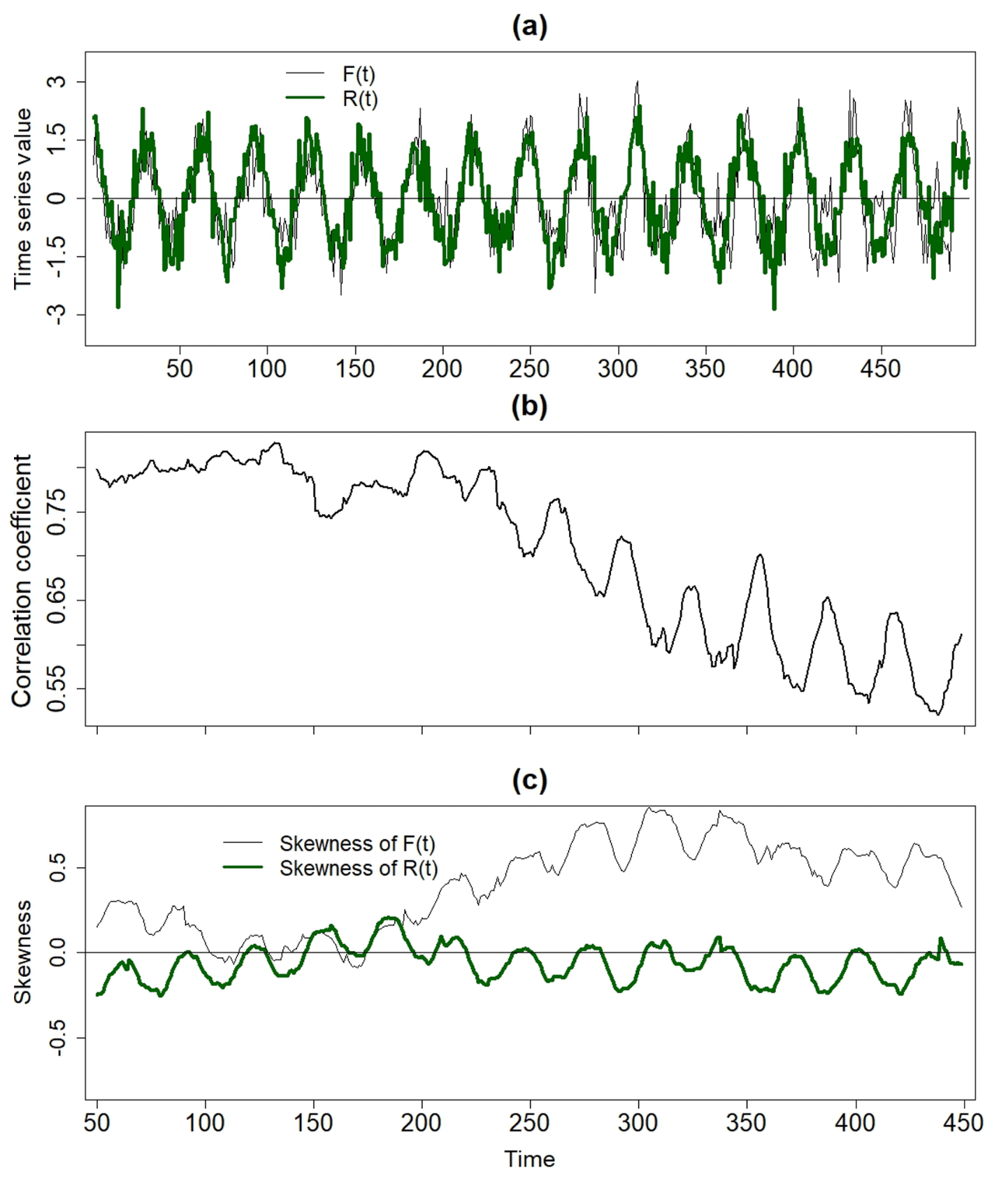
Figure 1 (a) An idealized nonlinear forcing time series, together with an idealized response R(t). The 120 point sliding correlation between F(t) and R(t). (c) The 120 point sliding skewness of F(t) and R(t).

An inspection of the local auto-bicoherence spectrum of F(t) (Fig. 2b) reveals that the auto-bicoherence at p₁=32 is increasing with time, indicating that the phase coupling between modes with periods p₃=16 and p₁=32 is strengthening with time. The biphase of 0^∘, as indicated by arrows pointing to the right, confirms that the quadratic-phase coupling is contributing to the positive skewness, seen in Fig. 1a, to an increasing degree. Furthermore, the nonlinear coherence between R(t) and F(t) is weak and mostly statistically insignificant at p₃=32 (Fig. 2c), implying the skewness of ${\mathit{\gamma }}_{\mathrm{16}}^{\mathrm{F}}+{\mathit{\gamma }}_{\mathrm{32}}^{\mathrm{F}}$ is uncorrelated with the skewness of ${\mathit{\gamma }}_{\mathrm{16}}^{\mathrm{R}}+{\mathit{\gamma }}_{\mathrm{32}}^{\mathrm{R}}$, where ${\mathit{\gamma }}_{\mathrm{16}}^{\mathrm{F}}+{\mathit{\gamma }}_{\mathrm{32}}^{\mathrm{F}}$ is the sum of the cosines in Eq. (16) and the components of W_F(t) at p₃=16 and p₁=32. The nonlinear mode ${\mathit{\gamma }}_{\mathrm{16}}^{\mathrm{R}}+{\mathit{\gamma }}_{\mathrm{32}}^{\mathrm{R}}$ is the sum of the cosine in Eq. (17) and the components of W_R(t) at p₃=16 and p₁=32. Thus, the skewness of R(t) in the time domain is practically uncorrelated with the skewness of F(t) because the skewness of F(t) is solely related to the phase coupling between the modes with periods p₃=16 and p₁=32. Thus, the increase in the skewness of F(t) also contributes to the weakening time-domain correlation.

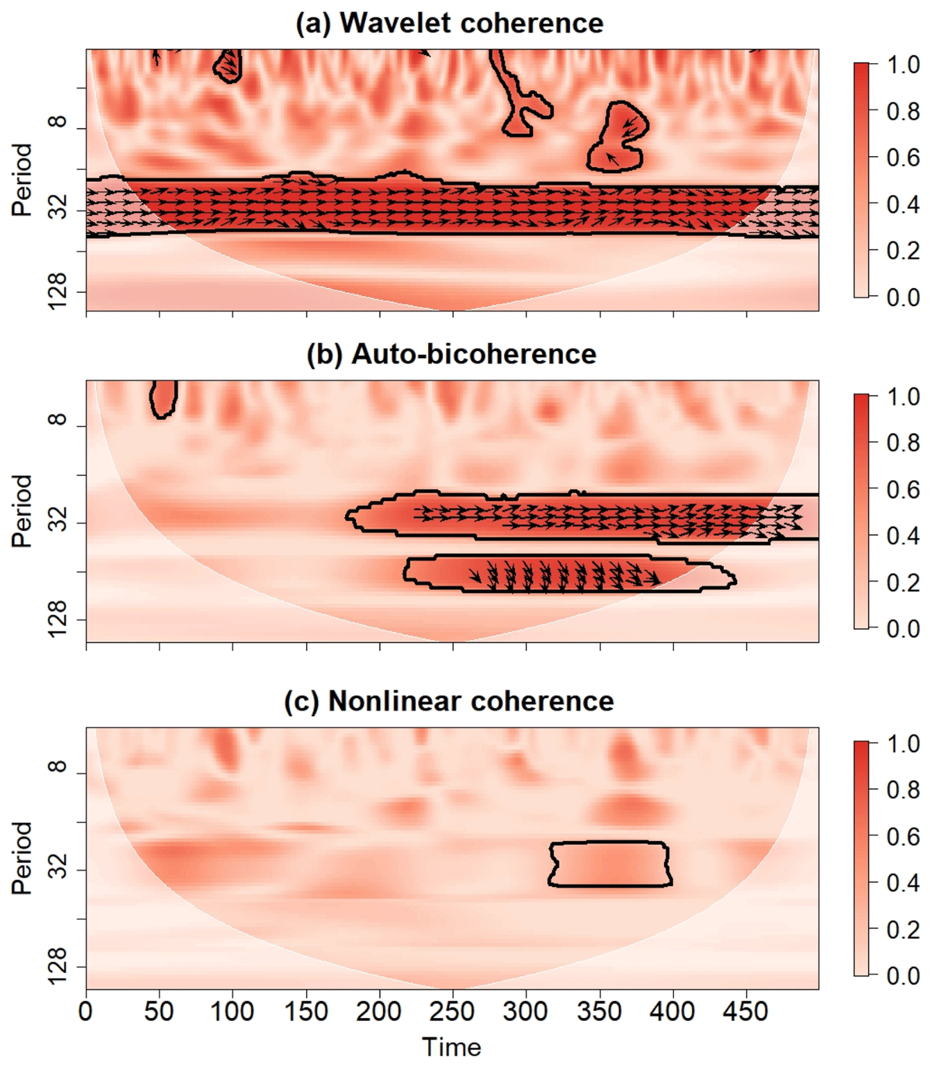
Figure 2 (a) Wavelet coherence between the time series of F(t) and R(t) as shown in Fig. 1. Arrows indicate the relative phase difference, where arrows pointing to the right mean that the time series are in phase. (b) The local diagonal slice of the auto-bicoherence spectrum of F(t). Arrows represent the biphase, where arrows pointing to the right mean that the quadratic-phase coupling between the mode with period indicated on the vertical axis and its harmonic contributes to positive skewness. (c) Nonlinear coherence between F(t) and R(t). Contours in all panels enclose regions of 5 % cumulative area-wise significance. The shaded region represents the cone of influence where edge effects may be important.

The lack of nonlinear coherence at timescales for which F(t) is nonlinear has implications for empirical prediction. At time points where F(t) is positively skewed, R(t) is overestimated because R(t) is not inheriting the skewness of F(t). That is, if one created a linear regression model based on the relationship between F(t) and R(t) from t=0 to t=200, one would find that a forcing value of, say, 1 would produce a response close to 1. If the same model was used to predict R(t) at, say, t=430, one would predict that the forcing with a value of around 2 should result in a response near 2. However, because the relatively large value F(430) results from skewness, and R(t) is uncorrelated with its skewness, the response is only as strong as the part of F(t) not resulting from the quadratic-phase coupling. The more nonlinear F(t) becomes, the more F(t) will overestimate R(t) when F(t) is positively skewed. Similarly, the positive forcing produces a negative response at t=450 because of skewness and not simply because of a change in variance. Nonlinear coherence allows for the quantification and identification of these time-domain aberrations.

The weakening relationship shown in Fig. 1b could lead a researcher studying a hydrological process to believe that another direct-forcing mechanism must be influencing the hydrological process. This belief could lead to the application of partial wavelet coherence (Ng and Chan, 2012) and partial correlation analyses to identify another influential forcing mechanism. However, in this case, there are no other direct-forcing mechanisms; the weakening time-domain relationship is solely related to how F(t) transitioned from a linear regime to a nonlinear regime. This theoretical result suggests that hydrological studies using wavelet coherence should also consider the nonlinearity of the times series.

4 Results

4.1 The ENSO and Indian monsoon time series and their time-domain relationship

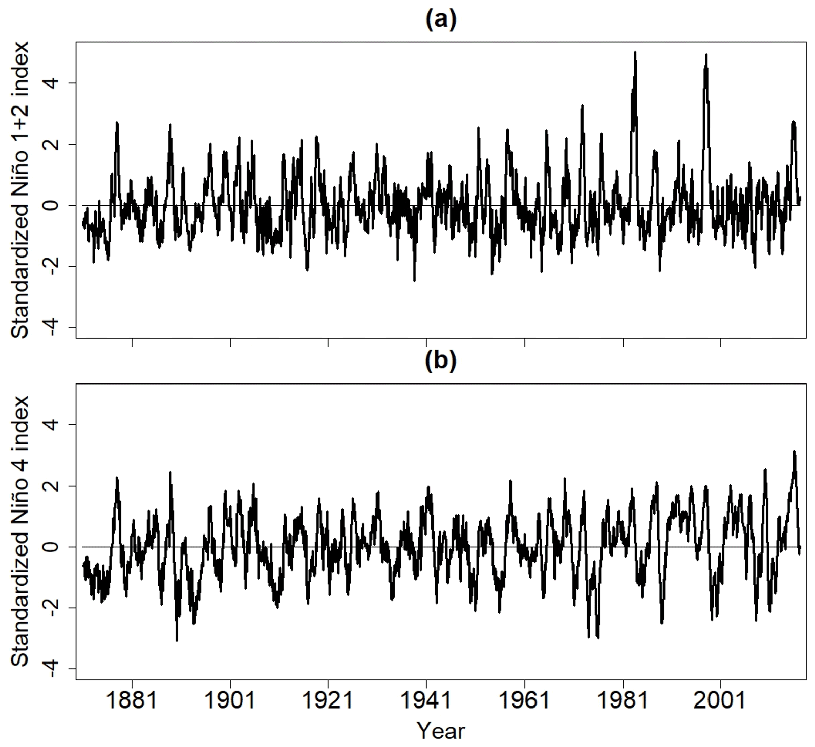
The contrasting Niño 1+2 and Niño 4 indices are shown in Fig. 3. For the Niño 1+2 time series (Fig. 3a), a few recent and notably intense warm events are located around 1982–1983, 1997–1998, and 2015–2016, coinciding with the strongest El Niño events in recent decades (McPhaden, 1999; Hu and Fedorov, 2017; Santoso et al, 2017). A few notably intense Niño 1+2 events are also seen in the 1800s, indicating that intense ENSO events are not unique to recent decades. An inspection of Fig. 3a also reveals that the recent intense warm Niño 1+2 events are also skewed in the sense that they are stronger than the surrounding cool Niño 1+2 events. Unlike the 1982–1983 and 1997–1998 Niño 1+2 events, the 1982–1983 and 1997–1998 warm events for the Niño 4 time series are unremarkable (Fig. 3b). Furthermore, cool Niño 4 events are preferentially stronger than warm events after the 1960s, suggesting an intensification of the negative skewness.

Figure 3 The time series of the (a) Niño 1+2 and (b) Niño 4 indices.

The 20-year sliding skewness time series of the Niño 1+2 index (Fig. 4) reveals enhanced skewness during the 1800s, near-zero skewness around the 1930s and early 1940s, and especially enhanced skewness after the 1970s associated with an upward trend in skewness beginning around the 1940s. In contrast to the Niño 1+2 index, the skewness of the Niño 4 index becomes more negative after the 1960s, and the magnitude of the skewness is generally smaller than that of the Niño 1+2 time series. This finding suggests that the transition of the Niño 1+2 time series to a nonlinear regime is more pronounced than the transition associated with the Niño 4 time series.

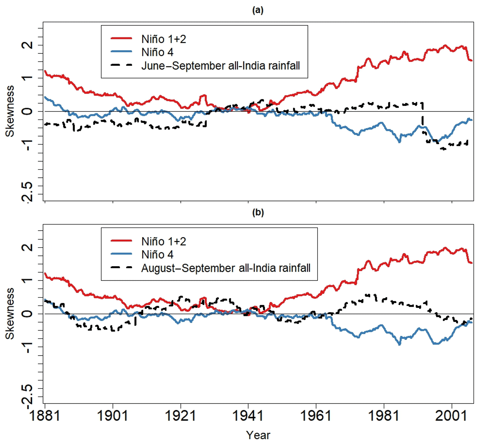
Figure 4 The 20-year sliding skewness of (a) June–September and (b) August–September all-India rainfall (AIR) and full time series for the Niño 1+2 and Niño 4 indices.

Interestingly, a 20-year sliding skewness analysis of AIR (Fig. 4) reveals that the skewness of June–September AIR remains close to zero until the 1990s, despite the upward trend in Niño 1+2 skewness beginning in the 1940s (Fig. 4a). Similarly, the skewness of August–September AIR does not increase to the extent that Niño 1+2 skewness does (Fig. 4b). On the other hand, the skewness of August–September AIR could be negatively correlated with the skewness of the Niño 4 index after the 1960s, consistent with how the August–September AIR and the Niño 4 index are negatively correlated. The skewness of June–September AIR becomes more negative in the 1990s and 2000s, but it is unclear if that negative skewness is related to ENSO, noise, or another climate pattern because the skewness of the Niño 1+2 and Niño 4 indices do not change as abruptly. Negative June–September AIR skewness is accompanied by enhanced positive skewness of the Niño 1+2 index prior to the 1940s, which is consistent with how June–September AIR is negatively correlated with the Niño 1+2 index during that time period (Fig. 5a).

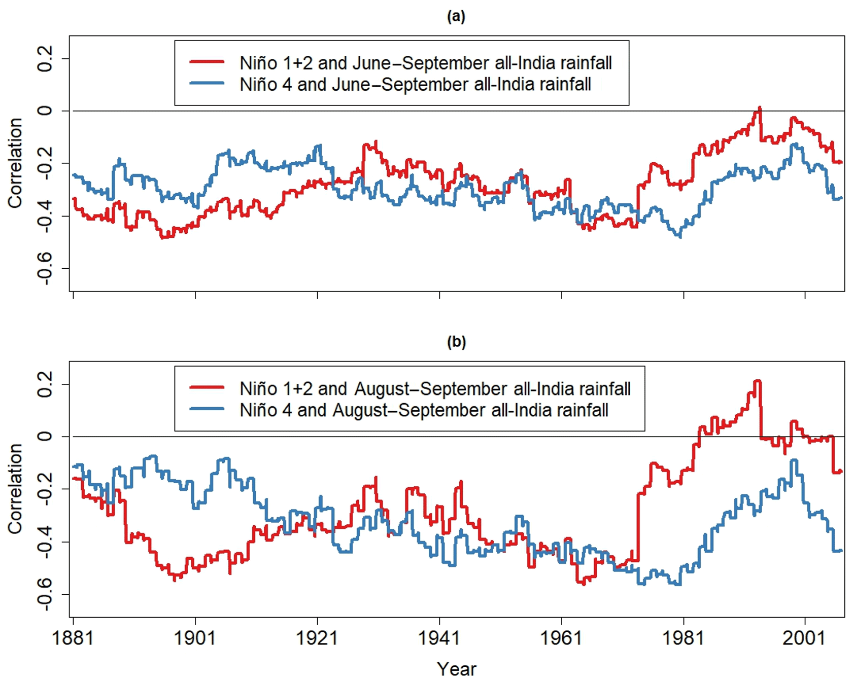
Figure 5 The 20-year sliding correlation between anomalies for June–September AIR, and the time series for the June–September Niño 1 and 2 and Niño 4 indices. (b) Same as (a) but for the August–September season.

The differences in skewness shown in Fig. 4 suggests that the correlation between the ENSO time series and AIR degrades after the 1970s, which is confirmed by the 20-year sliding correlation between the June–September AIR and ENSO time series (Fig. 5a). The relationship with the Niño 1+2 generally weakens from the 1800s to the 2000s. In contrast, the June–September AIR–Niño 4 index relationship appears to have no long-term trend, resulting in the Niño 4 index becoming more strongly correlated with AIR than the Niño 1+2 index after the 1970s.

The stronger AIR–Niño 4 index relationship compared to the AIR–Niño 1+2 index relationship after the 1970s is more evident in the August–September analysis (Fig. 5b). An abrupt weakening of the August–September AIR–Niño 1+2 index relationship occurs around the 1970s, with the relationship reversing around the 1990s. A comparison of Figs. 4b and 5b reveals that the weakening and reversal of the relationship occurs during the time period when the Niño 1+2 index is especially skewed. The difference in the magnitudes of Niño 1+2 and Niño 4 skewness after the 1970s could explain why the August–September AIR–Niño 1+2 index relationship weakens more abruptly than the AIR–Niño 4 index relationship. Thus, a further investigation is needed to better understand the temporal changes in ENSO statistics and their impact on the ENSO–AIR relationship.

4.2 Wavelet power analysis and coherence

The wavelet power spectra associated with the Niño 1+2 and Niño 4 time series (Fig. 6) reveal enhanced variance in the 16 to 64 month band after 1965 for all the time series. The appearance of holes in the contoured regions suggests that there are oscillatory modes with nearby frequencies (Schulte, et al., 2015), though the wavelet power spectra cannot determine if there is quadratic-phase coupling between the oscillatory modes.

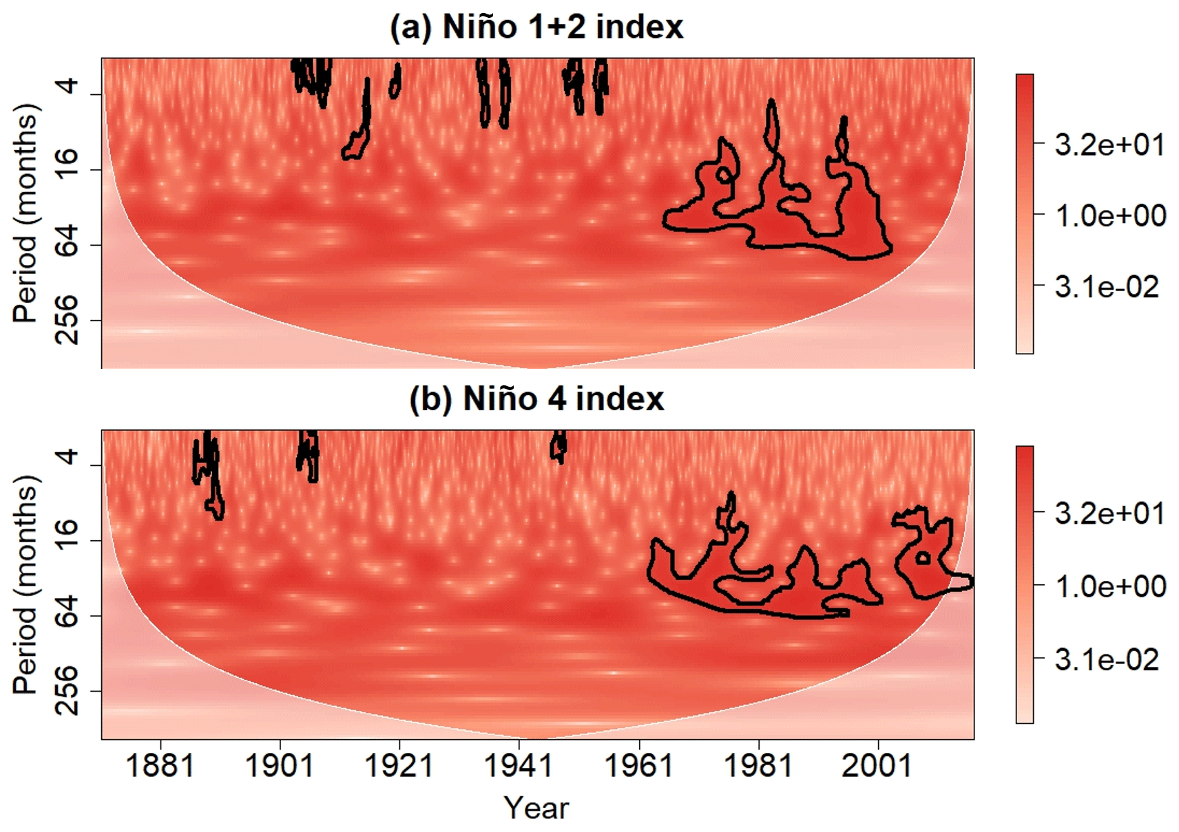
Figure 6 Wavelet power spectrum of the (a) Niño 1 and 2 and (d) Niño 4 indices. Contours enclose regions of 5 % cumulative area-wise significance. The shaded region represents the cone of influence, which is the region where edge effects are nonnegligible.

The linear wavelet coherence spectrum, shown in Fig. 7, indicates that the AIR relationship with the Niño 1+2 and Niño 4 indices in the 16 to 64 month band breaks down after 1995, which is consistent with the findings from the sliding correlation analysis shown in Fig. 5. The relationship between AIR and these ENSO indices also weakens around 1925, but this weakening does not appear in the sliding correlation analysis. Note that the lack of linear coherence after 1995 coincides with the enhanced ENSO variance (Fig. 6), implying that higher ENSO variance need not be associated with higher AIR variance at those timescales, so changes in ENSO variance could be contributing to the weakening ENSO–AIR time-domain correlation. However, ENSO skewness is also enhanced during this time period (Fig. 4), so the weakening relationships may not simply be related to ENSO variance. Thus, further analysis is needed to extract information unrevealed by the linear wavelet power and coherence methods.

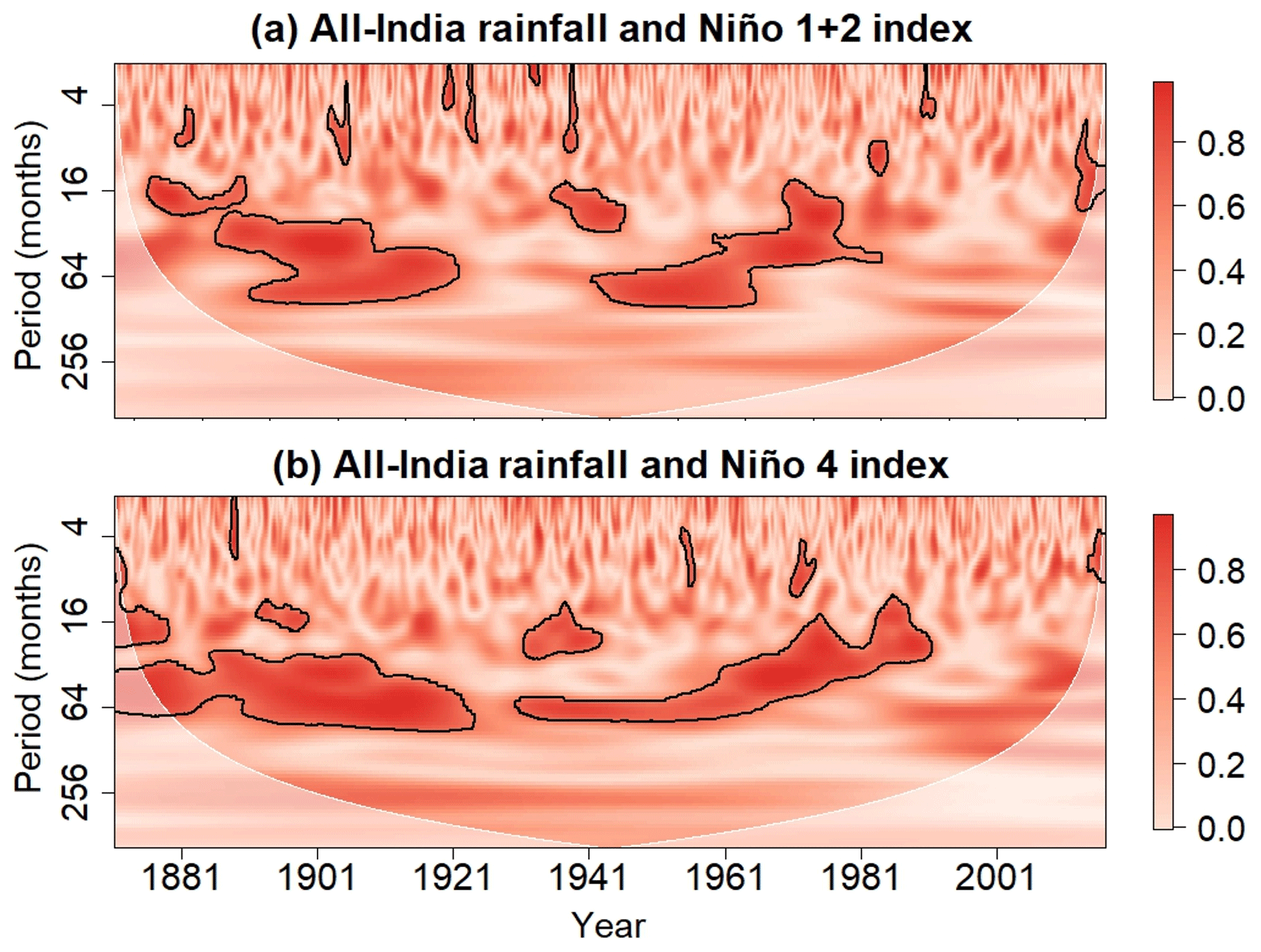
Figure 7 Wavelet coherence spectrum between AIR and time series for the (a) Niño 1 and 2 and (b) Niño 4 indices. Contours enclose regions of 5 % cumulative area-wise significance. The shaded region represents the cone of influence, which is the region where edge effects are nonnegligible.

4.3 Local auto-bicoherence of ENSO

Figure 8 shows that the local auto-bicoherence spectra of all ENSO time series contain statistically significant local auto-bicoherence, but the spectrum of the Niño 4 index is only associated with a few statistically significant regions, such as the one around 2015 at a period of 32 months. For the Niño 1+2 index, there is an intensification in the auto-bicoherence spectrum after the 1970s, which is consistent with the ENSO regime shift (Santoso et al., 2013). A comparison of Figs. 4 and 8 reveals that enhanced skewness coincides with stronger auto-bicoherence on the 32 to 64 month timescale, suggesting that the skewness partially arises from the stronger quadratic-phase coupling among oscillatory modes with periods ranging from 32 to 64 months.

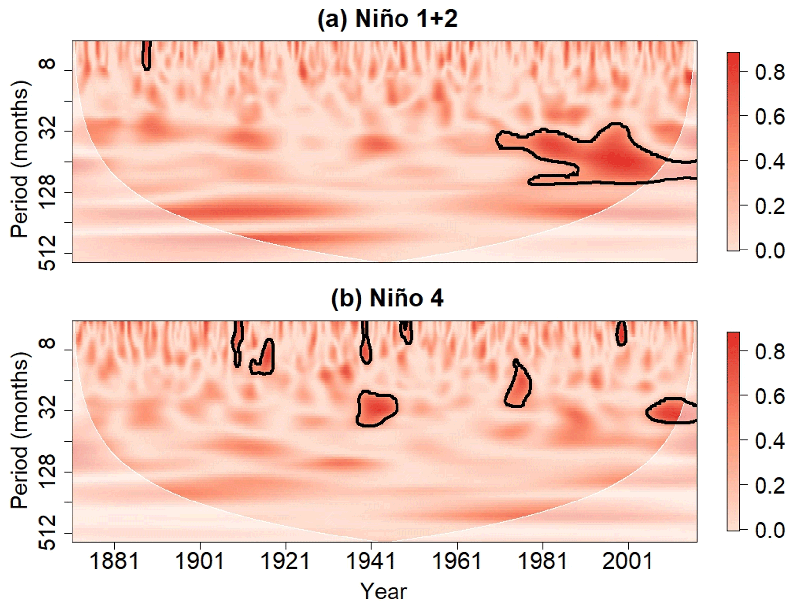
Figure 8 Local auto-bicoherence spectra of the (a) Niño 1 and 2 and (b) Niño 4 indices. Contours enclose regions of 5 % cumulative area-wise significance, and the shading represents the cone of influence.

To confirm that the nonlinear-phase coupling identified in Fig. 8 is associated with skewed waveforms, we inspected the corresponding local biphase spectra (not shown). It was found that the biphase in the 42 to 64 month band is generally 0^∘, so the nonlinear-phase coupling in that band contributes to the positive skewness of the 1982–1983, 1997–1998, and 2015–2016 events.

4.4 Nonlinear coherence between all-India rainfall and ENSO

The results shown in Fig. 9 indicate that the nonlinear wavelet coherence between AIR and the time series for the Niño 1+2 and Niño 4 indices is statistically significant in the 32 to 64 month band, mainly prior to the 1980s. The nonlinear coherence in this band appears to peak around the 1972–1973 El Niño event, indicating that an increase in the positive skewness of ENSO should tend to coincide with the enhanced negative skewness of AIR around this time. However, much of the statistically nonlinear coherence is located during the time period when ENSO is more linear than it has been in recent decades (Fig. 8), so the effects of the nonlinearities are small regardless of the nonlinear wavelet coherence. In contrast, the auto-bicoherence of the Niño 1+2 time series in the 32 to 64 month band is statistically significant and high after the 1970s (Fig. 8), so the lack of nonlinear coherence after the 1980s, shown in Fig. 9, is expected to impact the time-domain correlation more strongly, much like the theoretical situation shown in Figs. 1 and 2. Our results are consistent with this theoretical idea because the AIR–Niño 1+2 relationship weakens more than the AIR–Niño 4 relationship after the 1970s (Fig. 5), which is expected because the Niño 1+2 index is more nonlinear than the Niño 4 index during this time period. However, unlike the theoretical example shown in Fig. 2, the linear coherence between the ENSO time series and AIR also weakens around the 1990s (Fig. 7), so the weakening relationship could be the result of a combination of factors that includes ENSO nonlinearity.

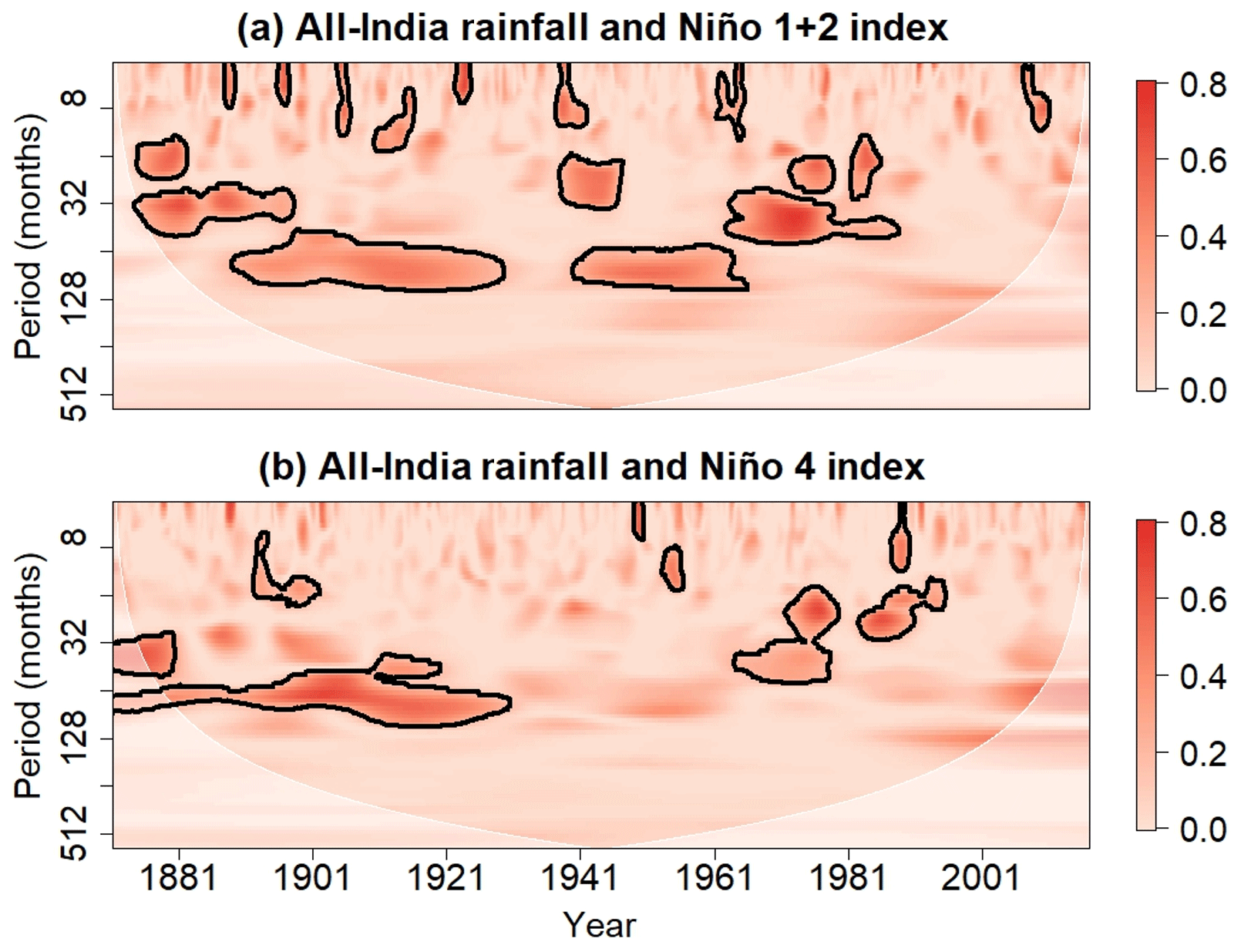
Figure 9 Nonlinear wavelet coherence between the full AIR time series and full times series for the (a) Niño 1 and 2 and (b) Niño 4 indices. Contours enclose regions of 5 % cumulative area-wise significance, and the shading represents the cone of influence.

The 20-year sliding mean of the ENSO auto-bicoherence, coherence, and nonlinear coherence averaged in the 32 to 64 month band further highlights the impact of ENSO nonlinearity. As shown in Fig. 10a, the sliding mean nonlinear coherence between the Niño 1+2 index and AIR fluctuates less than the linear coherence and reaches a clear global maximum around the 1970s before rapidly declining to a global minimum around the late 1990s when the Niño 1+2 index is very nonlinear. As shown in Fig. 10a, the Niño 1+2 auto-bicoherence peaks around the same time that the August–September AIR–Niño 1+2 index correlation is positive. In fact, the correlation between the sliding September–August AIR–Niño 1+2 correlation time series and the sliding Niño 1+2 auto-bicoherence time series is 0.81, much higher than the correlation with the linear coherence ($r=-\mathrm{0.11}$) and nonlinear coherence ($r=-\mathrm{0.34}$) time series. These results support the idea that the Niño 1+2 regime shift impacted the weakening time-domain correlation. On the other hand, the correlation between the Niño 4 auto-bicoherence and the August–September AIR–Niño 4 correlation time series is weak, so changes in the nonlinearity of the Niño 4 index are unlikely to contribute substantially to changes in the AIR–Niño 4 relationship. Nevertheless, this result agrees with theory that suggests that nonlinearity is only an important contributor when the time series is highly nonlinear, which is not the case for the Niño 4 index because of the low auto-bicoherence (Figs. 8b and 10b). Because the nonlinear coherence between AIR and indices for the Niño 1+2 and Niño 4 is weak (Figs. 9 and 10), the more pronounced change in the August–September AIR–Niño 1+2 correlation reflects the more intense increase in Niño 1+2 nonlinearity compared to that of the Niño 4 index in recent decades.

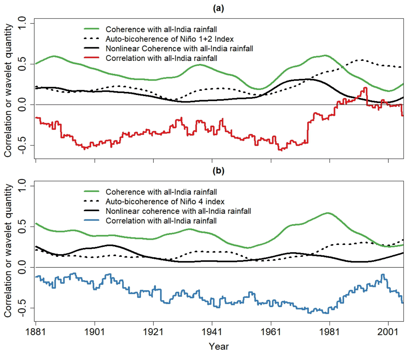
Figure 10 (a) The 20-year sliding mean time series of the linear wavelet coherence between AIR and the Niño 1 and 2 index, the auto-bicoherence of the Niño 1 and 2 index, and the nonlinear coherence between the Niño 1 and 2 index and AIR after they have been averaged in the band of 16 to 64 months. The red curve is the 20-year sliding correlation between the August–September Niño 1 and 2 index and AIR. (b) The same as (a) but for the Niño 4 index. The blue curve is the 20-year sliding correlation between the August–September Niño 4 index and AIR.

4.5 A possible explanation for the ENSO nonlinearity impacts

To better understand the association between ENSO nonlinearity and the AIR–ENSO relationship, the global auto-bicoherence spectra associated with the ENSO time series were first computed (Fig. 11). Then, the auto-bicoherence of SSTs associated with a few select peaks (p₁ and p₂) in Fig. 11 were computed at each grid point in the domain bounded by 20^∘ N and 20^∘ S and by 146^∘ E and 80^∘ W. The peaks were selected based on the auto-bicoherence spectra of the Niño 3.4 and Niño 1+2 indices. To select the peaks, local maxima in the auto-bicoherence within the statistically significance regions shown in Fig. 11 were identified, where points associated with local maxima were chosen because they were associated with the clearest patterns.

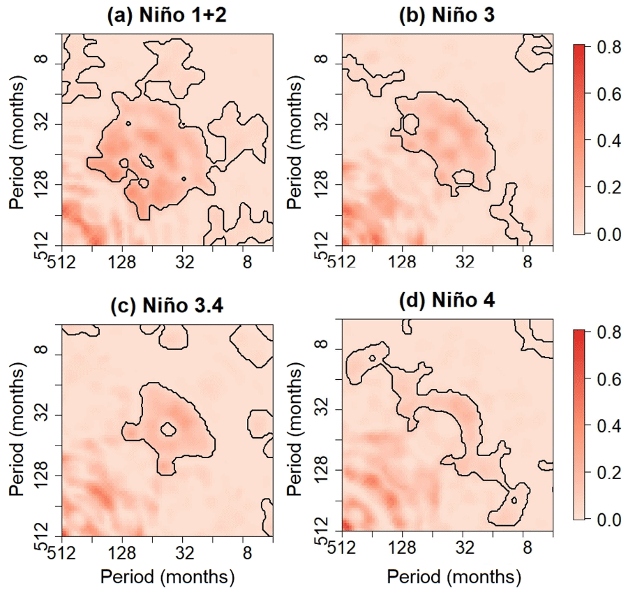
Figure 11 Global auto-bicoherence spectra of the (a) Niño 1 and 2, (b) Niño 3, (c) Niño 3.4, and (d) Niño 4 indices. Contours enclose regions of 5 % cumulative area-wise significance.

The spatial structure of global auto-bicoherence corresponding to the peaks in the Niño 3.4 auto-bicoherence spectrum are shown in Fig. 12. The auto-bicoherence associated with the pair (31, 31) is greatest across the central equatorial Pacific, with the overall spatial pattern being reminiscent of a central Pacific El Niño (Lee and McPhaden, 2010). This result suggests that the phase coupling between the 31 month mode and the 15.5 month mode could be related to the occurrence of central Pacific El Niño events (Sect. 5). In contrast, the auto-bicoherence pattern associated with the pair (56, 56) is more uniform, with auto-bicoherence slightly greater across the extreme eastern equatorial Pacific than the central equatorial Pacific. This pattern is reminiscent of an eastern Pacific El Niño. Like the pattern corresponding to the pair (31, 31), the auto-bicoherence for the pair (105, 57) tends to be greater across the central equatorial Pacific. Our findings suggest that different nonlinear modes contribute to different ENSO flavors. Although An and Jin (2004) and Burgers and Stephenson (1999) showed that the skewness is greatest across the eastern equatorial Pacific, we determined that such a time-domain approach is unable to capture frequency-dependent patterns in nonlinearity.

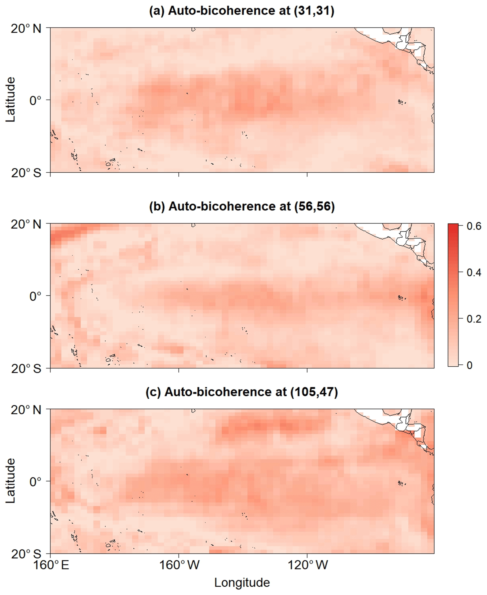
Figure 12 (a, b, c) Global auto-bicoherence corresponding to the monthly pairs, namely (31, 31), (56, 56), and (105, 47), respectively.

The spatial auto-bicoherence plots associated with the peaks in the Niño 1+2 auto-bicoherence spectrum are shown in Fig. 13. The auto-bicoherence associated with the pairs (148, 53) and (148, 105) is strong across the eastern equatorial Pacific but weak across the central equatorial Pacific, suggesting that the quadratic-phase coupling between the 148 and 105 month modes and between the 148 and 53 month modes is associated with the skewness of eastern equatorial Pacific SSTs. The pattern associated with the pair (62, 44) is reminiscent of an eastern Pacific El Niño, and the auto-bicoherence associated with the pair (88, 88) is relatively weak across the entire equatorial Pacific. A comparison of Figs. 12 and 13 shows that there is a tendency for auto-bicoherence to be greater across the eastern equatorial Pacific than the central equatorial Pacific, which is consistent with how SSTs across the eastern equatorial Pacific are most skewed (Burgers and Stephenson, 1999; An and Jin, 2004).

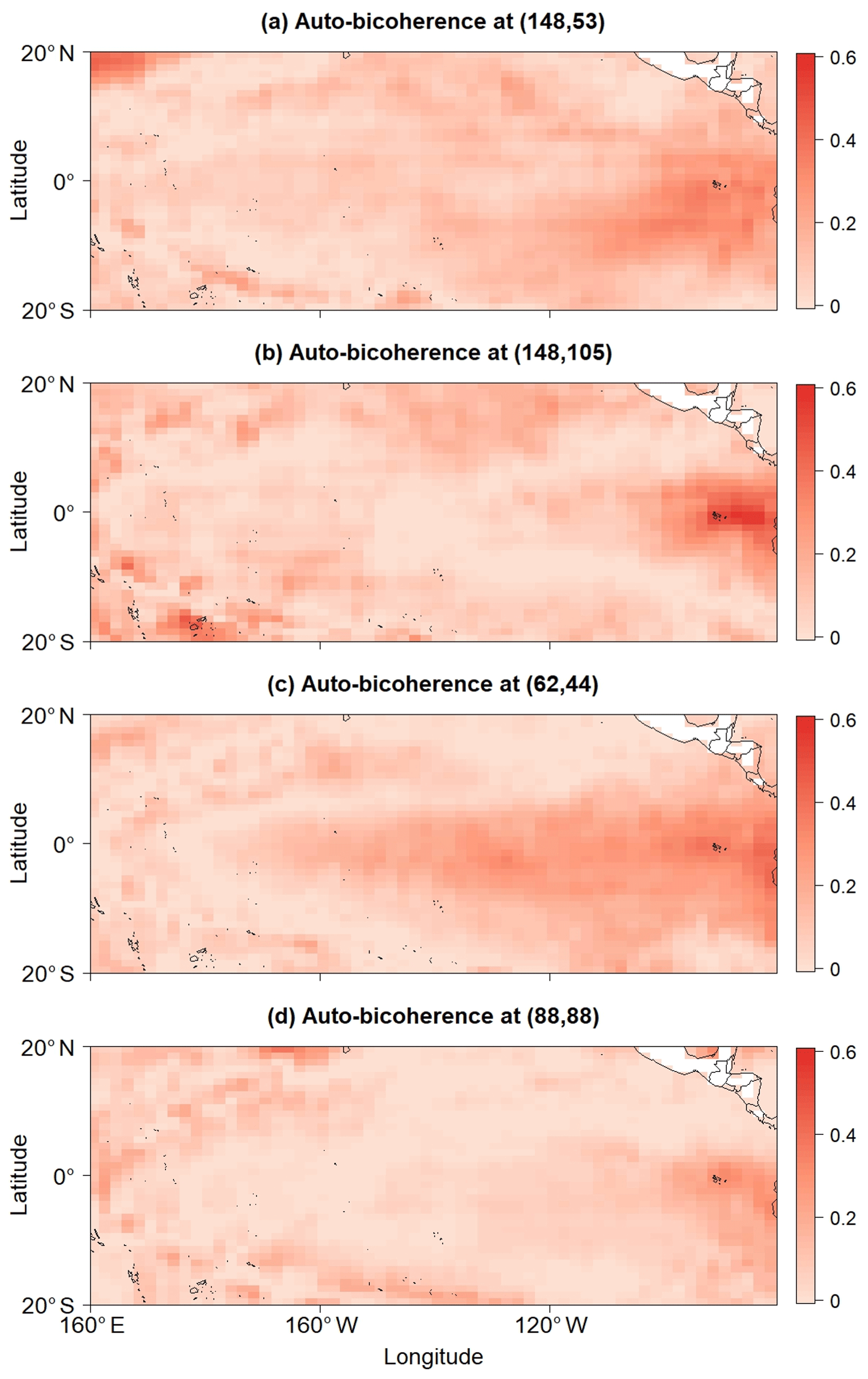
Figure 13 (a, b, c, d) Global auto-bicoherence corresponding to the monthly pairs, namely (158, 43), (148, 105), (62, 44), and (88, 88), respectively.

5 Discussion and conclusion

The nonlinear nature of ENSO was examined using higher-order wavelet methods. The auto-bicoherence spectra of the Niño 1+2 and Niño 4 indices time series revealed that ENSO skewness arose from the quadratic-phase coupling of modes with various periods. For the Niño 1+2 index, the quadratic-phase coupling after the 1970s was especially strong, which is consistent with how ENSO underwent a regime shift around the 1970s (Santoso et al., 2013) that was marked by an increase in ENSO skewness. Although the Niño 3.4 time series was not considered in detail in this study, an auto-bicoherence analysis of the time series (not shown) revealed phase coupling between modes with periods of 31 and 15.5 months in addition to coupling between modes with periods of 61 and 30.5 months. The phase coupling between the 31 and 15.5 modes was found to be especially strong after 1995, whereas the quadratic-phase coupling between the 61 and 30.5 month modes was found to intensify after the 1970s. These additional results suggest that nonlinear modes vary in intensity and time of occurrence.

The evolution of SSTs across the Niño 4, Niño 3.4, Niño 3, and Niño 1+2 regions was found to be nonlinear, but the degree to which the time series are nonlinear is different (Fig. 11). Overall, the Niño 1+2 time series were found to be the most nonlinear, while the Niño 4 index was found to be the most linear. The spatial patterns associated with the nonlinearities depend on the frequency components contributing to the nonlinearities. For example, the quadratic-phase coupling between the modes with periods of 31 and 15.5 months was found to be the strongest in the central equatorial Pacific and weakest across the eastern equatorial Pacific. This finding suggests that the more frequent occurrence of central Pacific El Niño events in recent decades (Lee and McPhaden, 2010) could be linked to the strengthening of this quadratic-phase coupling, which could explain the relationship between ENSO nonlinearity and changes in the ENSO–AIR relationship because central Pacific El Niño events have been shown to be more effective at creating drought-inducing subsidence over India (Kumar et al., 2006).

The results from the present and previous studies (Fan et al., 2017) support the idea that changes in the ENSO–AIR relationship are related to ENSO flavors because ENSO nonlinearity appears to be related to ENSO flavors (Figs. 12 and 13), which is in opposition to the findings of other work showing that the changes are related to sampling variability or to noise. According to Yun and Timmermann (2018), the changes in the time-domain correlation between AIR and ENSO are consistent with the assumption that AIR is the sum of the ENSO signal and Gaussian white noise (i.e., AIR = ENSO and white noise). However, for this hypothesis to hold, the difference in AIR–ENSO must be Gaussian white noise. As shown in this study, the nonlinear wavelet coherence between ENSO metrics and AIR is weak, and ENSO–AIR contains periodicities (Fig. S2), which means that AIR is not simply a stochastically perturbed ENSO signal as noise does not contain periodicities. The retention of non-Gaussian noise features was certainly the case for R(t)–F(t) in the example in Sect. 3.5 because the difference retains the cosine function with a period of 16.

The fact that nonlinear coherence between rainfall and ENSO is determined by linear coherence between ENSO and rainfall at two or three frequencies means that the changing time-domain correlation could be more fully understood by determining why linear coherence changes at the frequencies that contribute to ENSO skewness. Such an analysis could provide a more mechanistic perspective than the theoretical perspective adopted in this study. A preliminary analysis showed that there was enhanced linear coherence between the North Atlantic Oscillation index and AIR after 1995 in the 16 to 64 month band associated with ENSO nonlinearity. This result suggests that conditions across the North Atlantic (Kakade and Dugam, 2000; Bhatla et al., 2016) could influence the nonlinear coherence between ENSO and AIR and, thus, the corresponding time-domain correlation.

The tools used and developed in this study may have important applications for understanding how forecasting systems replicate Indian rainfall and its associated teleconnections. These methods, for example, could determine if forecasting systems can reproduce nonlinear characteristics of climate time series. As such, an R software package has been developed to implement these methods (available at: http://justinschulte.com/wavelets/advbiwavelet.html; last access: 22 November 2019). These methods could provide new directions for improving current forecasting systems and, ultimately, predictions of Indian rainfall.

Appendix A

The first step (Step 1) in assessing the cumulative-area significance of a point was the calculation of the N=12 sets as follows:

$$\begin{array}{}\text{(A1)}& P_{\mathrm{pw}}^i=\left\{\left(b,a\right):{\mathit{\rho }}_{\mathrm{pw}}\left(b,a\right)<{\mathit{\alpha }}_i\right\},\end{array}$$

where each set is the subset of the wavelet domain consisting of points for which the wavelet quantities are point-wise significant at the α_i level (i.e., the point-wise test p-value, ρ_pw, is less than α_i). In this paper, α₁=0.02, α₁₂= 0.18, and ${\mathit{\alpha }}_{i+\mathrm{1}}-{\mathit{\alpha }}_i=\mathrm{0.02}$. In the second step (Step 2), a geometric pathway about x was computed, where a geometric pathway is a nested sequence, as follows:

$$\begin{array}{}\text{(A2)}& P_{\mathrm{1}}^x\subseteq P_{\mathrm{2}}^x\subseteq \mathrm{\dots }\subseteq P_N^x,\end{array}$$

such that, in the following:

$$\begin{array}{}\text{(A3)}& P_i^x=\left\{\left(b,a\right):\left(b,a\right)\in P_{\mathrm{pw}}^i,\left(b,a\right)\sim x\right\}\end{array}$$

are path-components of $P_{\mathrm{pw}}^i$ containing x. The equivalence relation ∼ on $P_{\mathrm{pw}}^i$ makes two points in $P_{\mathrm{pw}}^i$ equivalent if they can be connected by a continuous path in $P_{\mathrm{pw}}^i$. The third step (Step 3) involved the calculation of the normalized area corresponding to $P_i^x$. The normalized area is defined as the patch area divided by the square of the mean-scale coordinate of the patch, where $A_i^x$ was assumed to be 0 if $P_i^x=\mathit{\varphi }$ or $P_i^x=\left\{x\right\}$. The critical area $A_i^{\mathrm{crit}}$ was obtained by computing the (1−α_c)th percentile of the null distribution of normalized areas corresponding to the significance level α_i, where α_c is the significance level of the cumulative area-wise test. The null distributions were constructed by generating 1000 patches at the α_i significance level under the null hypothesis of red noise. The final step (Step 4) was to compute the following:

$$\begin{array}{}\text{(A4)}& r^x={\displaystyle \frac{\mathrm{1}}{N}}{\sum }_{j=\mathrm{1}}^N{\mathit{\lambda }}_j^x,\end{array}$$

where ${\mathit{\lambda }}_i^x=$ 2 if $A_i^x/A_i^{\mathrm{crit}}\mathit{>}\mathrm{1}$ and ${\mathit{\lambda }}_i^x=$ 0 if $A_i^x/A_i^{\mathrm{crit}}\mathit{<}=\mathrm{1}$. The wavelet quantity at the point x was deemed statistically significant at the α_c cumulative area-wise level if r^x>1.

Appendix B

For p>1, the (p+1)th-order poly-spectrum of a time series X is given by the following:

$$\begin{array}{}\text{(B1)}& B_n^X\left(s_{\mathrm{1}},s_{\mathrm{2}},\mathrm{\dots },s_p\right)={\widehat{W}}_n^X\left(s_{p+\mathrm{1}}\right)\left({\prod }_{k=\mathrm{1}}^p{W}_n^X\left(s_k\right)\right),\end{array}$$

where

$$\begin{array}{}\text{(B2)}& {\displaystyle \frac{\mathrm{1}}{s_{p+\mathrm{1}}}}={\sum }_{k=\mathrm{1}}^p{\displaystyle \frac{\mathrm{1}}{s_k}}.\end{array}$$

The third-order poly-spectrum is the bispectrum, and the fourth-order poly-spectrum is the trispectrum (Collis et al., 1998) which identifies the frequency components contributing to kurtosis. The (p+1)th-order coherence between two time series is given as follows:

$$\begin{array}{}\text{(B3)}& \begin{array}{rl}& R_n^{\mathrm{2}}\left(s\right)=\\ & {\displaystyle \frac{{\left|S{s}_{\mathrm{smooth}}^{-\mathrm{1}}{B}_n^{\mathrm{XY}}(s_{\mathrm{1}},s_{\mathrm{2}},\mathrm{\dots },s_p)\right|}^{\mathrm{2}}}{S\left(s_{\mathrm{smooth}}^{-\mathrm{1}}{\left|B_n^X(s_{\mathrm{1}},s_{\mathrm{2}},\mathrm{\dots },s_p)\right|}^{\mathrm{2}}\right)S\left(s_{\mathrm{smooth}}^{-\mathrm{1}}{\left|B_n^Y\left(s_{\mathrm{1}},s_{\mathrm{2}},\mathrm{\dots },s_p\right)\right|}^{\mathrm{2}}\right)}},\end{array}\end{array}$$

where $B_n^{\mathrm{XY}}(s_{\mathrm{1}}{s}_{\mathrm{2}},\mathrm{\dots },s_p)$ is the (p+1)th-order cross spectrum given by the following:

$$\begin{array}{}\text{(B4)}& B_n^{\mathrm{XY}}\left(s_{\mathrm{1}},s_{\mathrm{2}},\mathrm{\dots },s_p\right)=B_n^X(s_{\mathrm{1}},s_{\mathrm{2}},\mathrm{\dots },s_p){\widehat{B}}_n^Y(s_{\mathrm{1}},s_{\mathrm{2}},\mathrm{\dots },s_p).\end{array}$$

When p=2, Eq. (B3) measures the local cross-correlation between skewness, and when p=3, the equation measures the local cross-correlation between kurtosis.