Estimation of rainfall erosivity based on WRF-derived raindrop size distributions

Soil erosion can cause various ecological problems, such as land degradation, soil fertility loss, and river siltation. Rainfall is the primary water-driven force for soil erosion, and its potential effect on soil erosion is reflected by rainfall erosivity that relates to the raindrop kinetic energy. As it is difficult to observe large-scale dynamic characteristics of raindrops, all the current rainfall erosivity models use the function based on rainfall amount to represent the raindrops' kinetic energy. With the development of global atmospheric re-analysis data, numerical weather prediction techniques become a promising way to estimate rainfall kinetic energy directly at regional and global scales with high spatial and temporal resolutions. This study proposed a novel method for large-scale and long-term rainfall erosivity investigations based on the Weather Research and Forecasting (WRF) model, avoiding errors caused by inappropriate rainfall–energy relationships and large-scale interpolation. We adopted three microphysical parameterizations schemes (Morrison, WDM6, and Thompson aerosol-aware) to obtain raindrop size distributions, rainfall kinetic energy, and rainfall erosivity, with validation by two disdrometers and 304 rain gauges around the United Kingdom. Among the three WRF schemes, Thompson aerosol-aware had the best performance compared with the disdrometers at a monthly scale. The results revealed that high rainfall erosivity occurred in the west coast area at the whole country scale during 2013–2017. The proposed methodology makes a significant contribution to improving large-scale soil erosion estimation and for better understanding microphysical rainfall–soil interactions to support the rational formulation of soil and water conservation planning.

1 Introduction

Soil erosion plays a pivotal role in shaping the Earth's physical landscape; however, it can threaten both ecosystems and human societies (Alewell et al., 2015). Accurate quantification of soil loss impact at large spatial scales is therefore important for developing land-use planning and sustainable conservation practices (Bilotta et al., 2012). The soil erosion rate is driven by a combination of factors, including rainfall, topography, soil characteristics, land cover, and land management applications (Wischmeier and Smith, 1958; Panagos et al., 2015b). Among these, rainfall is a driving force that accounts for a large proportion of soil loss throughout most of the world (Panagos et al., 2015b). The erosive force of rainfall with consequent runoff is represented as erosivity of rainfall. This is a crucial factor for estimating soil loss in large-scale soil erosion models, for instance, the Universal Soil Loss Equation (USLE, Wischmeier and Smith, 1978; or RUSLE, Renard et al., 1997), Limburg Soil Erosion Model (LISEM) (De Roo et al., 1996), and USLE-M (Kinnell and Risse, 1998).

Rainfall erosivity estimation involves the microphysical properties of rainfall and rainfall–soil interactions on different time steps (Petan et al., 2010). The impact of rainfall, the main mechanism driving the splashing of soil particles from the soil mass, which leads to soil erosion through soil disintegration and mobilization, relies on the kinetic energy (KE) of raindrop motions (Wischmeier and Smith, 1958; Wang et al., 2014). Robust measurement of raindrop size and terminal velocity is vital for estimating and predicting rainfall erosivity. Many measurements can be used to obtain these two parameters, including the stained paper or flour pellet methods (Marshall and Palmer 1948; Wischmeier and Smith, 1958), high speed cameras (Jones, 1959; Kinnell, 1981; McIsaac, 1990), and disdrometers (Petan et al., 2010; Angulo-Martinez et al., 2012). Accurate measurements of raindrop size can be provided in all their methods, and terminal velocity of raindrops can be further measured by video cameras and disdrometers. Velocity can also be estimated as the function of raindrop diameter from the empirical relationship (Beard, 1976; Atlas and Ulbrich, 1977; Uplinger, 1981; Van Dijk et al., 2002). When using ground observations, rainfall KE can be estimated at a given site.

However, direct measurement of rainfall KE in a large area is difficult because it requires considerable effort, as well as a dense network of expensive instruments that provide accurate outputs (Fornis et al., 2005; Mikoš et al., 2006; Meshesha et al., 2016; Dai et al., 2017). Previous studies have, therefore, mainly employed more readily accessible records like rainfall intensity and attempted to estimate rainfall KE from the empirical relationship of unit KE (ke) with intensity (ke–I). Since Marshall and Palmer (1948) first observed a two-parameter exponential relationship between drop size and intensity, several forms of ke–I mathematical expressions for specific locations and climatic conditions have been proposed, including power-law (Park et al., 1982; Meshesha et al., 2016), linear (Sempere-Torres et al., 1998; Nyssen et al., 2005), polynomial (Carter et al., 1974), logarithmic (Wischmeier and Smith, 1978; Davison et al., 2005; Meshesha et al., 2014), and exponential (Kinnell, 1981; Brown and Foster, 1987) relationships. Among these, the exponential function is preferentially used currently (Van Dijk et al., 2002; Fornis et al., 2005; Petan et al., 2010; Sanchez-Moreno et al., 2012; Lim et al., 2015). Accurate raindrop size distribution (DSD) measured by disdrometers is widely used to derive ke–I relationships (Angulo-Martínez et al., 2016; Meshesha et al., 2016). However, such empirically derived formulas indicate that rainfall ke will increase infinitely with increasing intensity, whereas studies (Rosewell, 1986; Angulo-Martínez et al., 2016; Meshesha et al., 2019) have found that rainfall ke reaches a top value when intensity is around 70 mm h⁻¹ (Hudson, 1963; Wischmeier and Smith, 1978). More importantly, such a ke–I relationship only represents local climate and precipitation microphysics and is valid for such regions. There is great uncertainty associated with rainfall erosivity estimation using this ke–I relationship in a large domain (Angulo-Martínez and Barros, 2015), especially due to the poor spatial and temporal predictability of the ke–I relationship. This has motivated researchers to directly calculate KE based on large-scale DSD measurements.

Ground- and space-based radar can be used to obtain DSD parameters (Atlas et al., 1973; Doelling et al., 1998). For example, the space-borne Dual-frequency Precipitation Radar (DPR) radar containing Ku- and Ka-bands in the Global Precipitation Measurement (GPM) satellite allows researchers to estimate the global three-dimensional spatial distribution of hydrometeors. Unfortunately, ground dual-polarization radars are available in limited areas (Prigent, 2010) with large uncertainties (Dai et al., 2019), and the GPM DPR instrument, which measures DSD with daily or longer temporal resolutions, fails to capture a full storm and meet the requirement for rainfall kinetic estimation. Mesoscale numerical weather prediction models, for instance, the WRF model, can simulate microphysical cloud processes and predict the evolution of particle size distribution through computationally feasible parametrization schemes (Dai and Han, 2014; Brown et al., 2016). DSD on the ground can be derived from the WRF model through consideration of various physical processes, types of hydrometeor, and free degrees of size distributions in hydrometeor. As such, a number of recent studies have investigated the retrieval and uncertainty of DSD parameters by WRF (Gilmore et al., 2004; Ćurić et al., 2009; Brown et al., 2016; Yang et al., 2019).

The WRF model runs with initial and boundary conditions using global reanalysis datasets, such as those of the European Centre for Medium-range Weather Forecasts (ECMWF) and National Centers for Environmental Prediction (NCEP). In other words, WRF-derived DSD can be obtained for any given area with fine spatial and temporal resolutions rather than traditional course linear interpolations. We therefore attempted to estimate rainfall erosivity for the entirety of the United Kingdom (UK) domain using WRF-derived DSD. For comparison, we also calculated interpolated traditional disdrometer-derived rainfall erosivity. To our knowledge, this work is the first attempt to take advantage of a numerical weather prediction model for estimating rainfall erosivity anywhere around the world. The current study contributes to the development of large-scale soil erosion estimation and provides a better comprehension of microphysical rainfall–soil interactions.

2 Methodology

2.1 Disdrometer-based rainfall KE estimation

KE dominates the ability of raindrops to separate soil particles. The KE (e, unit: J) of a raindrop with mass m (g) and terminal velocity v (m s⁻¹) is defined by the following:

$$\begin{array}{}\text{(1)}& e={\displaystyle \frac{\mathrm{1}}{\mathrm{2}}}m{v}^{\mathrm{2}}.\end{array}$$

Assuming a spherical volume for every raindrop shape, the mass of a drop can be calculated from the cube of the diameter D (mm). Because instruments (e.g., disdrometers) generally sample drop size, the mean radius and falling velocity of the corresponding sampling drop-size class are used to represent D and v, expressed as D_i and v_i, respectively. In such cases, the e_i with any drop of a given class is given as follows:

$$\begin{array}{}\text{(2)}& e_i={\displaystyle \frac{\mathrm{1}}{\mathrm{12}}}{\mathrm{10}}^{-\mathrm{6}}\mathit{\pi }\mathit{\rho }{v}_i^{\mathrm{2}}{D}_i^{\mathrm{3}},\end{array}$$

where ρ is the water density (g cm⁻³). The sum of the KE of each individual raindrop within a given rain depth that hits a given area defines the total KE. The unit rainfall KE ke_t in the tth minute (MJ ha⁻¹ mm⁻¹) can be calculated as the sum of each drop KE in each size set, as follows:

$$\begin{array}{}\text{(3)}& {\mathrm{ke}}_t={\displaystyle \frac{e_{\mathrm{sum}}}{A{P}_t}}={\displaystyle \frac{\mathrm{1}}{A{P}_t}}\sum _{i=\mathrm{1}}^{ni}{N}_i{e}_i,\end{array}$$

where A represents the sample area of the sensor, P_t is rainfall depth at time t, and N_i is the drop number in class i. The instrument sums up the number of raindrops in each sampling class and produces the raindrop spectra for a time step. Here, we use the term ke to represent the disdrometer-based KE estimated by DSD directly measured every minute. The terminal velocity of a raindrop can be estimated from its power-law empirical relationship with raindrop diameter (Atlas and Ulbrich, 1977), with this considered more suitable for Chilbolton in the UK (Islam et al., 2012):

$$\begin{array}{}\text{(4)}& v_{\mathrm{Atl}}=\mathrm{3.78}{D}_i^{\mathrm{0.67}}\end{array}$$

Thus, unit rainfall KE estimates per minute are obtained by replacing v_i in Eq. (2) with v_Atl.

The other form of rainfall KE is expressed at an event scale and represents the sum of the storm energy covering all time steps covering an event. The individual event energy (MJ ha⁻¹) is calculated as follows:

$$\begin{array}{}\text{(5)}& E=\sum _{t=\mathrm{1}}^{\mathrm{nt}}{\mathrm{ke}}_t{P}_t,\end{array}$$

where P_t is the rainfall amount (mm) in the tth minute and nt is the time step number. Historical rainfall data are divided into wet and dry periods. A string of erosive rainfall storms is first extracted through the predefined rules. A continuous 6 h dry-period interval was used to divide rainfall events (Hanel et al., 2016), following the “minimum dry-period duration” definition of a rainfall event (Bonta, 2004). Moreover, a rainfall amount of 12.7 mm was set as the threshold to filter effective rainfall events (Renard et al., 1997).

Rainfall KE is obtained for a given site based on size and velocity of raindrops. When disdrometer data are absent, energy can be estimated from empirical relationships using rainfall intensity I (mm). Five commonly used functions (including exponential, logarithmic, power law, and inverse proportion) have been mentioned in Section 1. Taking the exponential form as an example, the rainfall KE at any location can be estimated as follows:

$$\begin{array}{}\text{(6)}& E_{max}=e_{max}\left(\mathrm{1}-a{e}^{-bI}\right),\end{array}$$

where e_max is the mean maximal value of energy measured under high rainfall intensity, and a and b are coefficients modelling the equation curve. Here, minimum KE can be determined by parameters a and e_max together, while the overall shape of the curve is modelled by parameter b.

2.2 WRF-based rainfall KE estimation

Differing from disdrometer measurements, the complete DSD cannot be obtained from the WRF model. Instead, the DSD of the microphysical parameterization (MP) scheme is handled with a constrained-gamma distribution model, which is defined as follows:

$$\begin{array}{}\text{(7)}& N\left(D\right)=N_{\mathrm{0}}{D}^{\mathit{\mu }}{e}^{-\mathit{\lambda }D},\end{array}$$

where N₀, μ, and λ are the intercept, shape, and slope parameters of the DSD. In terms of double-moment bulk schemes, N₀ and λ can be abstracted from the number concentration N and predicted mixing ratio q, as shown below:

$$\begin{array}{}\text{(8)}& {\displaystyle }{N}_{\mathrm{0}}={\displaystyle \frac{N{\mathit{\lambda }}^{u+\mathrm{1}}}{\mathrm{\Gamma }(\mathit{\mu }+\mathrm{1})}},\text{(9)}& {\displaystyle }\mathit{\lambda }={\left[{\displaystyle \frac{cN\mathrm{\Gamma }(\mathit{\mu }+d+\mathrm{1})}{q\mathrm{\Gamma }(\mathit{\mu }+\mathrm{1})}}\right]}^{\frac{\mathrm{1}}{d}}.\end{array}$$

c and d are the assumed power-law coefficients between diameter and mass (m=cD^d), and Γ represents the function in gamma form (Morrison et al., 2009). The value of the shape parameter μ (μ=0) in double-moment schemes is fixed, except for the WRF double-moment 6-class (WDM6) schemes, following gamma distribution, which defined μ=1 (Jung et al., 2010; Johnson et al., 2016).

Because DSD retrieval is sensitive to MPs (Cintineo et al., 2014; Morrison et al., 2015), the WRF model in this study completely or partially incorporates three types of double-moment cloud MP schemes. The Morrison double-moment scheme involves the number concentrations and mixing ratios of multiple hydrometeors (Morrison et al., 2009). Moreover, the WDM6 scheme further considers a prognostic factor to estimate and predict the cloud condensation nuclei (CCN) number concentration (Hong et al., 2010; Lim and Hong, 2010). Finally, the Thompson aerosol-aware (TAA) scheme can predict both ice nuclei (IN) and CCN number concentrations (Thompson and Eidhammer, 2014).

The DSD parameters were thus obtained under the three WRF MPs. For theoretical DSD, ke estimates per minute were obtained by integration of the full raindrop size spectrum using the following:

$$\begin{array}{}\text{(10)}& {\mathrm{ke}}_t^{\prime }={\displaystyle \frac{\mathrm{1}}{A{R}_t}}\underset{\mathrm{0}}{\overset{\mathrm{\infty }}{\int }}N\left(D\right){\displaystyle \frac{\mathrm{1}}{\mathrm{12}}}{\mathrm{10}}^{-\mathrm{6}}\mathit{\pi }\mathit{\rho }{v}_i^{\mathrm{2}}{D}_i^{\mathrm{3}}\mathrm{d}D.\end{array}$$

For the WRF-derived DSD covering the whole study area, there was no need to construct a ke–I relationship to interpolate KE in ungauged areas. The WRF-based rainfall KE under storm event scale is thus given as follows:

$$\begin{array}{}\text{(11)}& E_{\mathrm{W}}=\sum _{t=\mathrm{1}}^{\mathrm{nt}}{\mathrm{ke}}_t^{\prime }{P}_t.\end{array}$$

2.3 Rainfall erosivity estimation

Most storm events have relatively low intensities and KEs with occasional peaks, based on the disdrometer DSD data used to evaluate the rainfall ke–I function. Proper estimation of rainfall erosivity potential should consider total KE over a long period. The rainfall erosivity factor (or R factor) is calculated by a multi-annual average of the total storm erosivity index (Wischmeier and Smith, 1958; Van Dijk et al., 2002), while annual rainfall erosivity R can be obtained using the following:

$$\begin{array}{}\text{(12)}& R=\sum _{m=\mathrm{1}}^M{\left({\mathrm{EI}}_{\mathrm{30}}\right)}_m,\end{array}$$

where M is the total number of erosive events within a year. (EI₃₀)_m denotes total rainfall kinetic energy and maximum 30 min rainfall intensity recorded within 30 consecutive minutes (unit: mm h⁻¹), respectively, for the mth event.

Wischmeier and Smith (1958) first proposed the use of EI₃₀, as the rainfall erosivity for each event, based on research data from many sources. I₃₀ was calculated to have higher relevance to soil erosion than maximum 5, 15, or 60 min rainfall intensities (Wischmeier and Smith, 1958). The calculation of EI₃₀ initially uses recording-rain gauge data to divide continuous rainfall into time periods with equal rainfall intensity. Though rainfall measurements with high temporal resolutions are required, it is difficult to obtain them from general rainfall measurements. Therefore, short-time equal-interval rainfall data with higher accuracy over multiple years are preferred for estimating EI₃₀. For example, Xie et al. (2016) used 1 min rainfall data instead of recording-rain gauge records. For coarse-resolution, equally spaced data, researchers have proposed a conversion factor to reduce bias error (Weiss, 1964; Williams and Sheridan, 1991).

The rainfall erosivity can be derived from rainfall KE. It plays a main dynamic role in USLE/RUSLE, representing the potential for soil erosion caused by rainfall. To distinguish the disdrometer- and WRF-derived rainfall erosivity in this study, we use the terms R_D and R_W, respectively.

2.4 Evaluation methods

Because there is no direct way to measure rainfall erosivity across a large area, it is difficult to validate outcomes using observations. However, R_D is considered to be relatively accurate due to its specific measurement of raindrops. We therefore assumed that R_W values were accurate if they closely matched R_D of a given location. A long-term comparison of R_W and R_D at disdrometer stations was thus conducted to evaluate the validity of R_W.

Three indicators were introduced for the evaluation: Pearson's correlation coefficient, mean absolute error (MAE), and coefficient of determination (R²) (Borrelli et al., 2017). The Pearson correlation coefficient is an index used to evaluate the linear correlation between two variables and is defined as follows:

$$\begin{array}{}\text{(13)}& \begin{array}{rl}& \mathrm{Pearson}=\\ & {\displaystyle \frac{n\sum R_{{\mathrm{D}}_i}\sum R_{{\mathrm{W}}_i}-\sum R_{{\mathrm{D}}_i}\sum R_{{\mathrm{W}}_i}}{\sqrt{n\sum R_{{\mathrm{D}}_i}^{\mathrm{2}}-{\left(\sum R_{{\mathrm{D}}_i}\right)}^{\mathrm{2}}}\sqrt{n\sum R_{{\mathrm{W}}_i}^{\mathrm{2}}-{\left(\sum R_{{\mathrm{W}}_i}\right)}^{\mathrm{2}}}}},\end{array}\end{array}$$

where n is the number of variable samples. Because this correlation cannot reveal the absolute bias of rainfall erosivity values, the MAE was also used; this is defined as follows:

$$\begin{array}{}\text{(14)}& \mathrm{MAE}={\displaystyle \frac{\sum \left|R_{{\mathrm{W}}_i}-R_{{\mathrm{D}}_i}\right|}{n}}.\end{array}$$

R² is an indicator to assess the fit of the trend line, expressed as the ratio of the variance in the dependent variable predicted from the independent variable. It measures the extent to which the model replicates observations based on the proportion of the results interpreted by the model to the total change, written as follows:

$$\begin{array}{}\text{(15)}& R^{\mathrm{2}}=\mathrm{1}-{\displaystyle \frac{{\mathrm{SS}}_{\mathrm{res}}}{{\mathrm{SS}}_{\mathrm{tot}}}},\end{array}$$

where SS_res is the sum of squares of residuals between two variables, and SS_tot is the total sum of squares.

3 Study area and data sources

The whole of the UK was set as the experimental area for investigating rainfall erosivity estimation. The UK consists of mostly lowland terrain, with a maximum elevation of 1345 m. Water and wind are the most significant forces of soil erosion in the UK. Together, they cause approximately 2.2 million tons of topsoil to be eroded annually, seriously affecting soil productivity, water quality, and aquatic ecosystems through siltation of watercourses (Environment Agency, 2004). According to the Environmental Agency, the total cost of soil erosion in the UK is approximately USD 88 million each year, including an agricultural production loss of USD 17.6 million (O'Neill, 2007). More importantly, the changing climate may exacerbate the degree of erosion. For example, hotter, drier climates make soils more susceptible to wind erosion, and intense storms increase rainfall erosivity (Defra, 2009). Studies of water erosion in England and Wales (Morgan, 1985; Evans, 1990) have found that loose soils (especially sand), such as the soils found in Shropshire and Herefordshire in Wales, are more susceptible to water erosion. In a study of rainfall erosion in Europe, Panagos et al. (2015a) found that the humid Atlantic climate results in highly variable rainfall erosivity, such as higher R factor values in western England and lower values in the eastern UK.

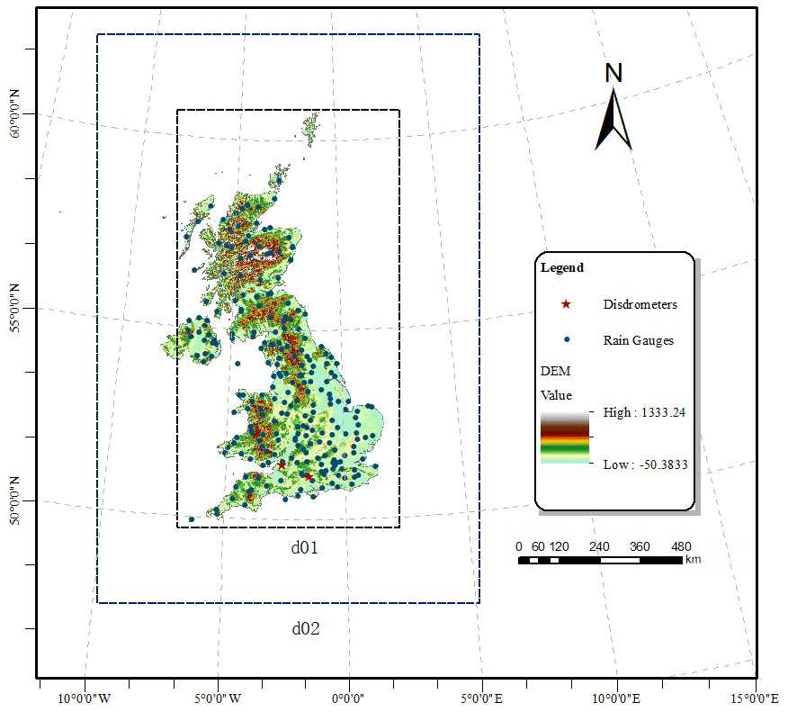
Figure 1 Location of rain gauges, Joss–Waldvogel disdrometer (JWD) at Chilbolton Observatory, OTT Parsivel² disdrometer (OPD) at Bristol Observatory and configurations of domain set-ups in the WRF model.

The gauge datasets used are from the land surface and marine surface measurements datasets (data availability: 1853–present) provided by the UK Met Office. A network of rain gauges covering 304 stations across the whole UK observes continuous rainfall data in hours (Fig. 1). The base data of most stations comprise the times of each tip (0.2 mm per tip), converted into 1 h rain accumulations. The rainfall observations are not always valid for each hour at each station. The hourly grid-based rainfall maps are then calculated based on ordinary kriging interpolation of rain gauge network data to obtain the spatial distribution of rainfall for each time step, as inputs for rainfall erosivity estimation. This wide-range-use geostatistical approach can account for both the distance and pairwise spatial relationship between points through variograms. The precipitation interpolation method uses sample gauge points taken at different locations and creates a continuous surface to achieve an accurate spatial variation estimation of rainfall patterns.

We used data from two disdrometers in southern England. The first was Chilbolton station (51^∘08^′ N, 1^∘26^′ W), with an impact-type Joss–Waldvogel disdrometer (JWD) mainly used to compute rainfall erosivity. It can measure drop sizes from 0.3 to 5.0 mm in 127 bins. The sampling period and collector area were 10 s and 50 cm², respectively. Data were available for April 2003 to July 2018. The second was the University of Bristol station (51^∘27^′ N, 2^∘36^′ W), with an OTT Parsivel² disdrometer (OPD). Data were available for November 2015 to December 2018. This disdrometer subdivides particles into appropriate classes and has a nominal cross-sectional area of 54 cm². The 10 s period measurement data from the two disdrometers were averaged into a 1 min period to filter out time variations (Montopoli et al., 2008; Islam et al., 2012; Song et al., 2017).

Meteorological data come from the ERA-Interim dataset, a global atmosphere re-analysis product, generated by the ECMWF. For the scientific community, ERA-Interim is considered to be one of the most important atmospheric datasets, with its data-rich period available since 1979 and updated in current time (Dee et al., 2011). The Integrated Forecasting System released in 2006 contains a 12 h window-derived 4-D variational analysis, driving the data assimilation system to generate ERA-Interim. The dataset covers 60 vertical classes of approximately 80 km from the ground to 0.1 hPa. The gridded binary format is used to store data for 3 months in a separate file. A data processing scheme was established to collect and retrieve ERA-Interim data of each rainfall event.

The rain gauge and Chilbolton disdrometer datasets can be obtained from British Atmospheric Data Centre in the National Centre for Atmospheric Science research centre (Meteorological Office, 2012). ERA-Interim data can be obtained from the ECMWF Public Dataset website (https://apps.ecmwf.int/, last access: 15 November 2020). Considering the availability of the above datasets and model requirements, we mainly used data covering the period 2004–2017.

4 Results

4.1 Empirically derived rainfall erosivity estimation

To evaluate the R_W, the raindrop spectrum collected by the Chilbolton station disdrometer is used to estimate rainfall KE first. The key to estimating rainfall KE by disdrometer lies in building an empirical relationship between rainfall amount and KE. We used DSD measurements from 2004 to 2013 to establish five empirical relationships between unit rainfall kinetic energy (ke) and intensity (I) (Table 1) and used 2014–2017 data for the cross-validation. It can be seen from Table 1 that the inverse proportional relationship (Eq. III) had the worst performance, in that both the calibration and validation R² values were < 0.3. The values of the other equations were > 0.48, among which the exponential formula (Eq. I) had the highest calibration R² (0.50) and validation R² (0.45), respectively. In addition, the power-law formula (Eq. V) showed a similar performance to the exponential formula at rainfall intensities < 5 mm h⁻¹. However, the power-law formula also had a continuously increasing trend, which may not be suitable for high intensities. Figure 2 shows the ke–I relationship and five fitted curves at Chilbolton station. It can be seen that the two logarithmic curves (Eqs. II and IV) invariably overlap. The logarithmic form has been used for a long time in USLE (Wischemier and Smith, 1978). It describes ke well at both low and high I but does not have an upper limit. The power-law curve (Eq. V) can predict ke well at lower I but overestimates ke at high I. The exponent-based relationship (Eq. I) is widely used in the literature and in forecast models such as RUSLE (Renard et al., 1997), which fits the data particularly well in Fig. 2. Even though ke in an exponential curve has a minimum value at very low I, it also should be noted that higher rainfall intensities are much more important in determining overall storm energy than lower intensities. Therefore, we adopted it here as the empirical formula to estimate rainfall erosivity in the UK.

Table 1 Relationship of ke–I at Chilbolton Station (2004–2013).

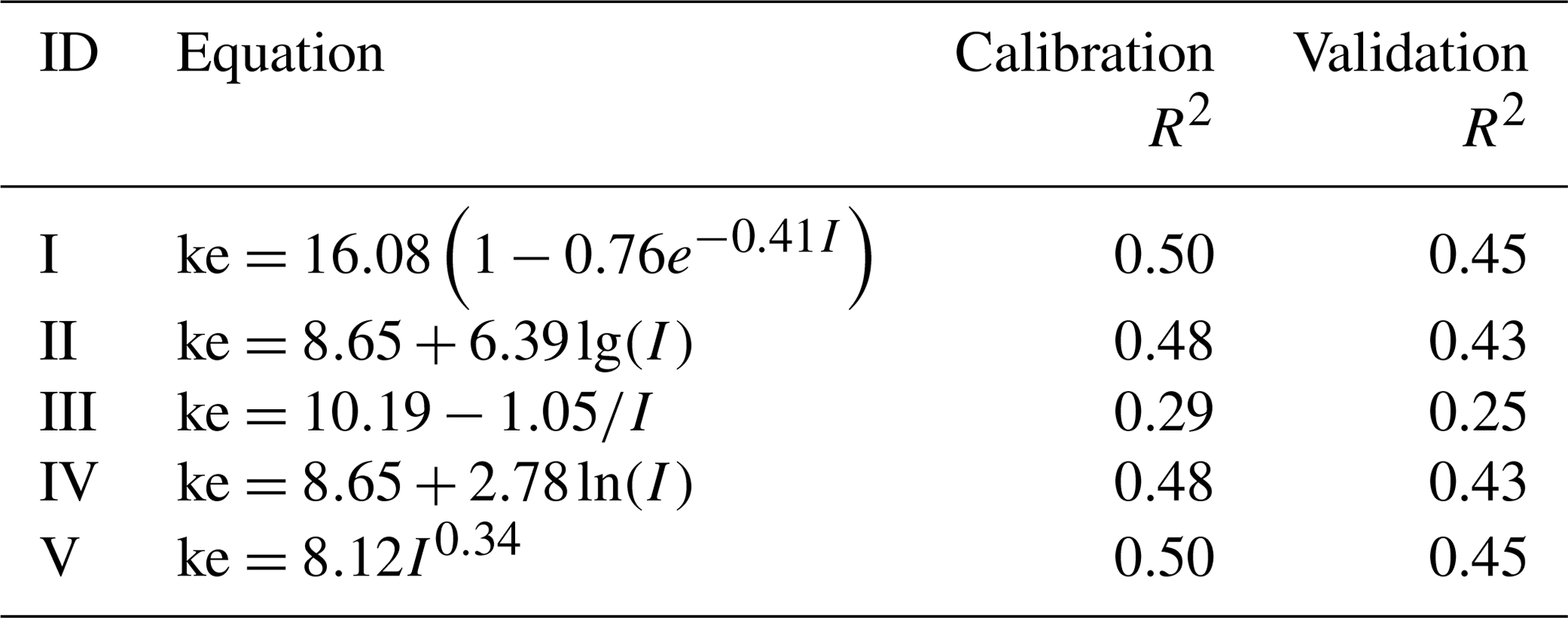
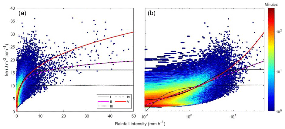
Figure 2 Number of minutes per intensity class (x axis) and ke class (y axis) with five fitted ke–I curves at Chilbolton station (2004–2013), plotted on linear (a) and logarithmic (b) intensity scales.

Based on rainfall KE, the point R_D can be obtained at a disdrometer location. In the current study, we established a method to estimate the R using 60 min rainfall data. EI₃₀ obtained from 1 min DSD data was considered as the standard R at Chilbolton Station. Hourly rain gauge data at the same location were used to calculate (EI₃₀)₆₀, which refers to EI₃₀ calculated from 60 min data. The regression relationship between EI₃₀ and (EI₃₀)₆₀ was then established. The (EI₃₀)₆₀ of each month, obtained from the 60 min rainfall data of the Chilbolton Station rain gauge in 2004–2013, was calculated. The regression relationship between the monthly sum of (EI₃₀)₆₀ and the standard monthly EI₃₀ from DSD was calculated to obtain a coefficient of 1.836. Rainfall erosivity can subsequently be calculated by multiplying (EI₃₀)₆₀ by the coefficient.

Figure 3 Gauge-based interpolation maps of annual rainfall amount (Rain), rainfall kinetic energy (E), and rainfall erosivity (R) in 2013–2017.

Beyond assuming that the disdrometer-derived ke–I relationship can be applied to a whole study area, point rainfall measurements must be interpolated to obtain areal rainfall values in traditional rainfall erosivity estimation. We obtained 60 min rainfall data from 304 rain gauges around the UK from 2004 to 2017. Note that not all rain gauges were available for the whole period (available gauges each year are indicated in Fig. 3). We used the ordinary kriging interpolation method to obtain the spatial distribution of rainfall for each time step. This wide-range-use geostatistical approach can account for both the distance and pairwise spatial relationship between points through variograms. Figure 3 shows the results of annual rainfall (Rain), annual rainfall kinetic energy (E), and annual rainfall erosivity (R) for different years. The distribution trends of Rain, E, and R were similar and positively correlated except for certain locations or periods. For instance, in 2013, Rain in the northwestern UK decreased from west to east, while E and R decreased from south to north; furthermore, areas with large E and R values in the southeastern UK could not be directly observed from the rain map.

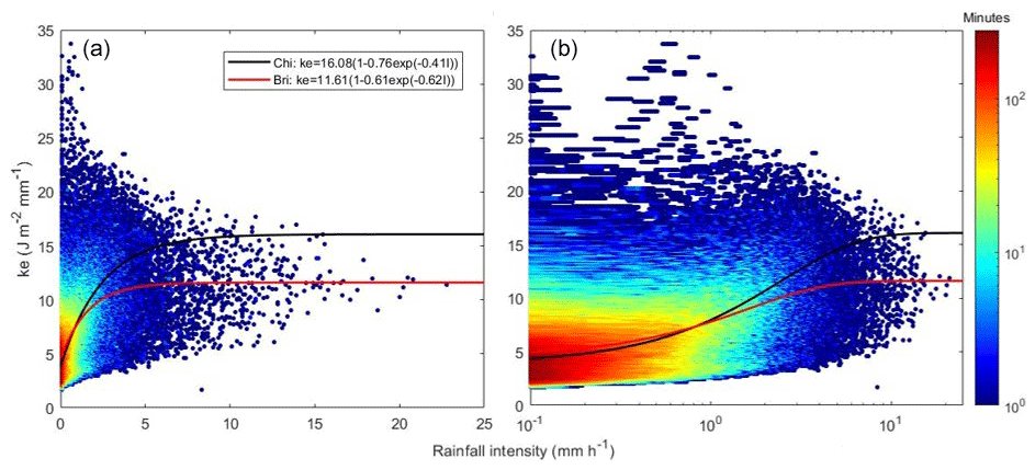
Figure 4 Minutes number per intensity class (x axis) and ke class (y axis) with fitted ke–I curves at Bristol station (2015–2018), plotted on linear (a) and logarithmic (b) intensity scales.

The key concern in traditional rainfall erosivity estimation is the spatial predictability of the ke–I relationship. To verify the regional reliability of this relationship, we used data from a newer disdrometer located at the University of Bristol, approximately 87 km from Chilbolton Station. The validation data at Bristol Station discontinuously covered the period 2016–2019. Figure 4 shows the exponential relationship of ke–I at Bristol station, which differed substantially from that based on data from Chilbolton station. A comparison of the modelled and observed event rainfall erosivity is shown in Fig. 5. The modelled erosivity of rainfall event was not consistent with the observed event rainfall erosivity. The linear regression coefficient between these values was > 1.2, which was the result of the low ke for Bristol Station, and R² was < 0.85, indicating considerable uncertainty associated with disdrometer-based rainfall erosivity estimation.

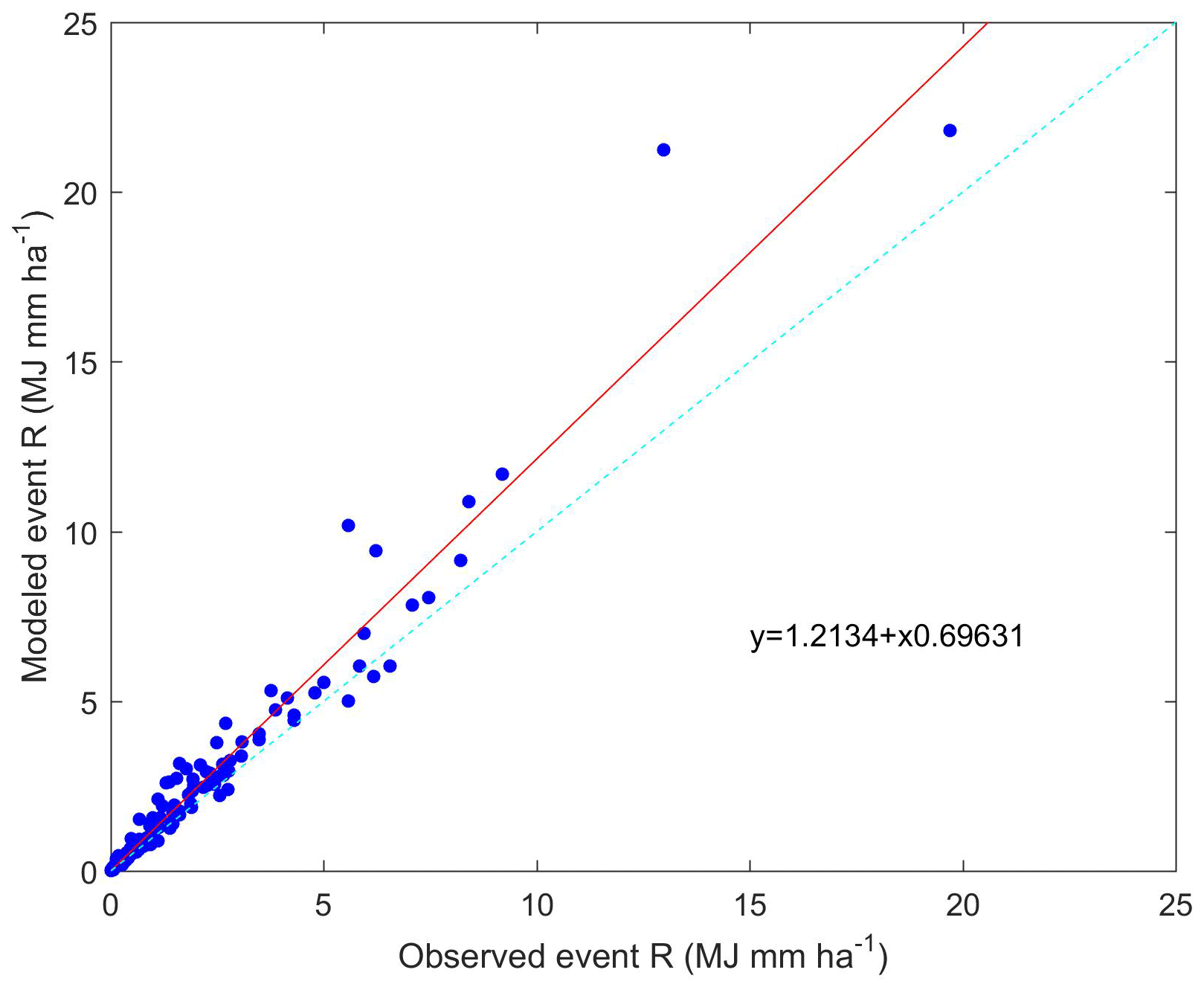
Figure 5 Comparison of observed and modelled event rainfall erosivity at Bristol Station, covering the period of 2016–2019.

In summary, the point rainfall erosivity estimated by disdrometer is considered to be accurate compared to other methods. However, a large-scale rainfall erosivity through a simple interpolation of rainfall KE is subjected to a significant uncertainty. In the following analysis, the point R_D is used to appraise the performance of the proposed WRF-based estimated method, and the R_D in the whole UK is only used for a general comparison of spatial and temporal distribution of rainfall erosivity.

4.2 Rainfall and DSD estimation by WRF

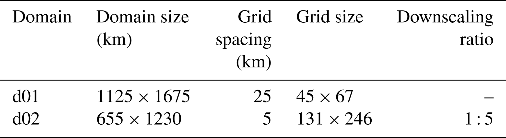
We used the WRF model version 3.8, which has an Advanced Research WRF dynamical core, to downscale the ERA-Interim reanalysis data. The double-nested domain configuration used in the WRF model was centred at 55^∘19^′ N, 2^∘21^′ W and applied at a downscaling ratio of 1 : 5, a finest grid of 5 km, and a temporal resolution of 1 h. Table 2 lists the detailed parameters used in this domain configuration. With the top pressure level set at 50 hPa in each, both domains include 28 vertical levels. To obtain favourable initial weather conditions, the model ran continuously to obtain 5 years of WRF simulation results.

Table 2 The configurations of the WRF model for two nested domains.

Simulations were performed using three different bulk double-moment MPs: the Morrison (Morrison et al., 2009), WDM6 (Hong et al., 2010; Lim and Hong, 2010), and TAA (Thompson and Eidhammer, 2014) schemes. All three can predict the number concentration and hydrometeors mixing ratio for each time step. The WDM6 scheme also predicts the number concentration of CCN (Hong et al., 2010; Lim and Hong, 2010), while the TAA scheme is able to predict both IN and CCN number concentrations (Thompson and Eidhammer, 2014). Additionally, other physical parameterizations include the Dudhia shortwave radiation scheme (Dudhia, 1989), Mellor–Yamada–Janjic planetary boundary layer scheme (Janjić, 1994), RRTM longwave radiation scheme (Mlawer et al., 1997), Noah land-surface model (Ek et al., 2003), and Kain–Fritsch cumulus scheme (Kain, 2004).

The median volume diameter parameter (D₀) and generalized intercept parameter (N_W) are generally used in the DSD model of WRF (Islam et al., 2012).

$$\begin{array}{}\text{(16)}& {\displaystyle }{N}_{\mathrm{W}}={\displaystyle \frac{N_{\mathrm{0}}{D}_m^{\mathit{\mu }}}{f\left(\mathit{\mu }\right)}},\text{(17)}& {\displaystyle }f\left(\mathit{\mu }\right)={\displaystyle \frac{\mathrm{6}(\mathrm{4}+\mathit{\mu }{)}^{\mathit{\mu }+\mathrm{4}}}{{\mathrm{4}}^{\mathrm{4}}\mathrm{\Gamma }(\mathit{\mu }+\mathrm{4})}},\end{array}$$

where D_m is the mass-weighted mean diameter. The f(μ) is a function of the shape parameter μ. The parameter μ is assumed as zero or one (based on microphysical scheme configuration) in WRF. Figure 6 displays the spatial distribution of D₀ and generalized intercept parameter N_W for a given day with rainfall countrywide (January 10, 2013). D₀ and N_W had similar patterns and were mainly distributed across the southwestern and northeastern UK. The white strip in the middle of the maps in Fig. 6 represents an area that received no rain. However, the three MPs yielded large differences; D₀ of MP-TAA was the highest among three MPs, whereas N_W of MP-WDM6 was significant larger than the others. In addition, D₀ and N_W did not consistently show a positive correlation. The different MP estimation results underscore the complexity of the rainfall process, which is the reason we estimated rainfall KE using WRF schemes instead of traditional formulas.

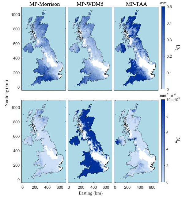
Figure 6 Map of average WRF DSD D₀ and N_W (10 January 2013).

4.3 Comparison of WRF- and disdrometer-derived rainfall erosivity at Chilbolton station

With the WRF-based rainfall intensity and DSD estimations, rainfall erosivity was derived using Eqs. (10)–(12). Hereafter, this is referred to as R_W, which is further distinguished based on the three MP schemes used: R_W-Morrison, R_W-WDM6, and R_W-TAA. Figure 7 compares disdrometer- and WRF-derived monthly rainfall erosivity estimations at Chilbolton station for the period 2014–2017. The general patterns of the four rainfall erosivity values were similar. R_W-Morrison tended to be larger than R_D in some months, whereas R_W-TAA matched the R_D value relatively well for smaller values. Because WRF data were taken from a 2 km × 2 km grid around Chilbolton station, there was a spatial error in addition to the systematic error of estimating rainfall erosivity. Based on the 4-year data, the study area is rainy throughout the year with little monthly R, or seasonal pattern changes (Fig. 8), influenced by the temperate oceanic climate. Figure 8 also indicated that through the perspective of monthly average results, R_W-WDM6 values are low, R_W-TAA has a good similarity with low R_D, and R_W-Morrison is the closest to R_D in value.

Figure 7 Comparison of disdrometer- and WRF-derived monthly rainfall erosivity estimations at Chilbolton station (2014–2017).

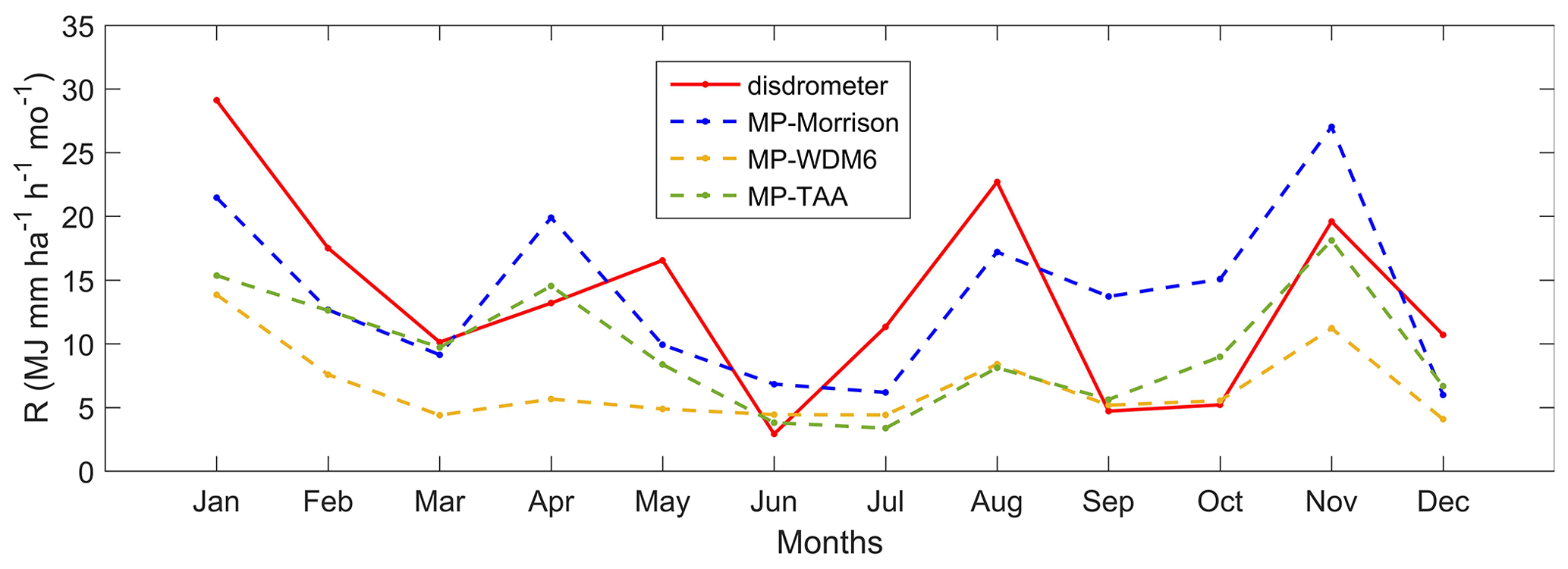
Figure 8 Comparison of disdrometer- and WRF-derived average monthly rainfall erosivity estimations at Chilbolton station (2014–2017).

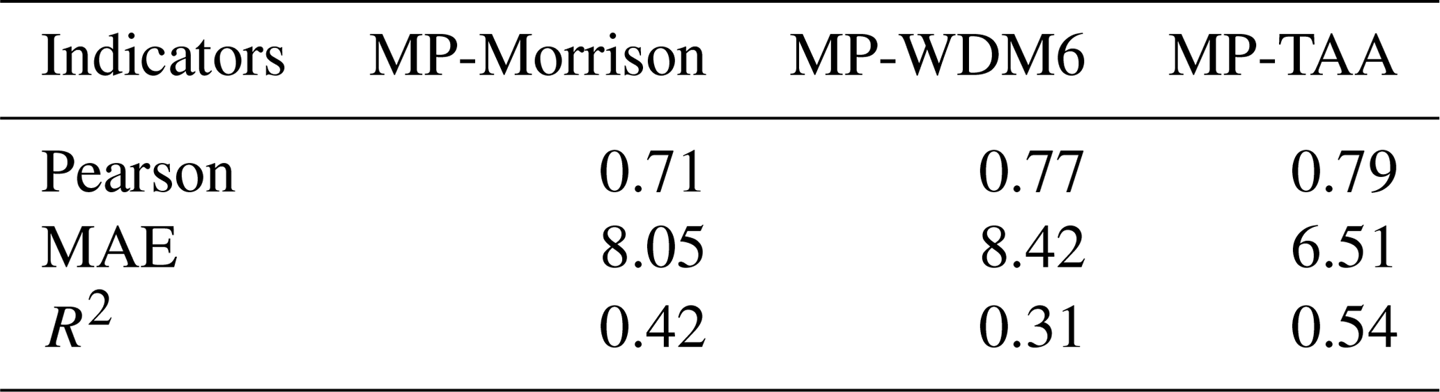
Table 3 shows the correlation indicator results between monthly R_D and the three types of R_W at Chilbolton station. The Pearson correlation coefficients generally exceeded 0.7, supporting the potential utility of WRF-based estimation. In terms of MAE, R_W-TAA had the best performance (6.51), whereas R_W-Morrison and R_W-WDM6 showed slightly worse performance (approximately 8). Among the three schemes, R_W-TAA had the best fit with R_D. The indicators and comparison results suggest that the deviations in results need to be considered; therefore, a method of bias elimination is described in Sect. 4.4.

Table 3 Indicator comparison between disdrometer-derived rainfall erosivity R_D and three types of WRF-derived rainfall erosivity at Chilbolton station on monthly scale (2014–2017).

4.4 R_W estimation for the whole UK

The R_W at Chilbolton station showed obvious systematic deviations compared with the disdrometer-derived results (see Sect. 4.2 and 4.3). Simple bias correction was therefore applied to adjust the individual storm KE estimations of R_W. The biases from dividing average R_W-Morrison, R_W-WDM6, and R_W-TAA by average R_D during 2014–2017 were 0.55, 0.20, and 0.36, respectively.

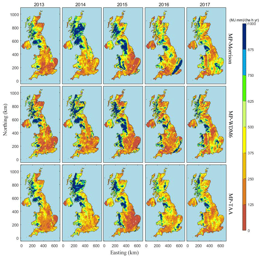
Figure 9 WRF-derived annual rainfall erosivity maps of the whole UK for different years.

The rainfall erosivity distribution for the whole UK was then obtained. Figure 9 shows the distribution of R_W at the annual scale covering the period 2013–2017. The pattern of the rainfall erosivity maps showed a general regional-dominant characteristic. For example, it always decreased from west to east, predominantly shaped by orography. Affected by the prevailing westerly winds, there was abundant rainfall in the western and northern mountains, as indicated by high rainfall KE values in these regions. In addition, among the study years, 2014 and 2015 showed higher national rainfall erosivity, with a large range in the west coast area.

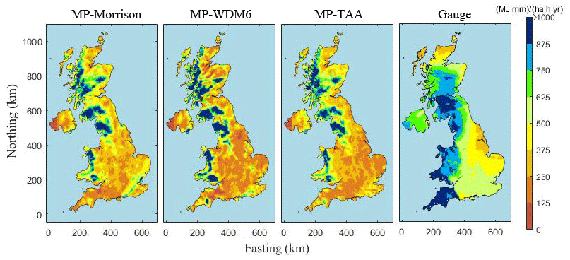
Figure 10 The 5-year (2013–2017) average annual rainfall erosivity maps based on WRF grids and rain gauge interpolation.

Figure 10 shows the average R distribution for 2013–2017 estimated by rain gauges and WRF MPs. WRF grids could cover all regions in the UK evenly, offering more detailed erosivity results, especially in the mountainous northwestern region. Here, values of an average-R map calculated by rain gauges were much higher than three types of R_W, although they all have R that decreased from west to east. Note that the ke–I empirical equation at Chilbolton station, used in the whole UK, will not always be accurate in regions with different rainfall characteristics. In terms of R_W results, the three MPs obtained the same spatial pattern in rainfall erosivity, where R_W-WDM6 yielded the greatest geographical difference. It is clear that the proposed WRF-based estimated method can capture more details of the spatial change of rainfall erosivity compared with the traditional disdrometer-based method.

The highest rainfall erosivity regions in the UK are concentrated in the mountainous areas along the western coast, related to their rainfall system. The moist air brought by the prevailing westerly wind from the Atlantic Ocean moves from west to east across the UK and rises when it encounters the mountains of western England. Therefore, the mountainous regions along the UK western coast have the highest rainfall amount and rainfall erosivity in the UK. In addition, western Scotland is under the subpolar oceanic climate, which enhances its humidity. On the contrary, eastern Scotland and northeastern England are more likely to be exposed to continental polar air mass, which brings dry and cold air and lower rainfall erosivity.

To evaluate the change in rainfall erosivity with time in the UK, the average value of all the WRF grids covering the whole UK was calculated over 2013–2017 (Fig. 11). The average R_W trends of R_W-Morrison and R_W-TAA were similar, both increasing from a minimum in 2013 to a maximum in 2014 and then gradually decreasing from 2014 to 2017. The red line in Fig. 11 indicates a series of mean values of the three MPs results, which varied from 367.82 to 516.00 MJ mm ha⁻¹ h⁻¹ yr⁻¹ (mean: 432.16 MJ mm ha⁻¹ h⁻¹ yr⁻¹).

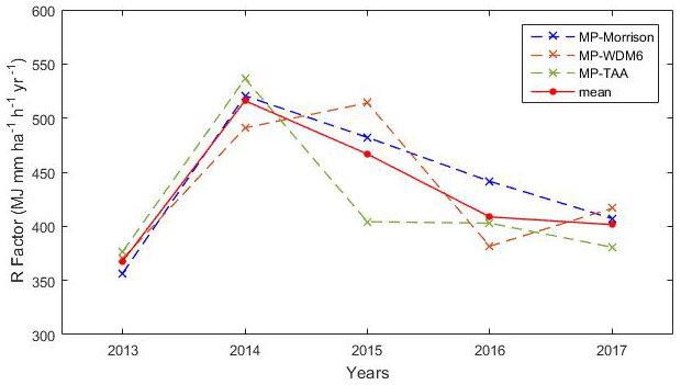
Figure 11 WRF-derived average annual rainfall erosivity of all the WRF grids covering the whole UK (2013–2017).

The maximum values for R_W-Morrison and R_W-TAA occurred in 2014, whereas that of R_W-WDM6 occurred in 2015. A sequence of extreme weather events occurred in the UK in 2014, including major winter storms in late January to mid-February, which caused widespread flooding and other economic losses and greatly increased rainfall erosivity that year. However, the gauge-based interpolation map shows the average annual rainfall amounts for the years 2013–2017 were 884.9, 1014.0, 1008.5, 894.9, and 937.3 mm, respectively. The large rainfall erosivity difference between 2014 and 2015 and the 2 years with similar rainfall amount indicate that much rainfall erosion occurs during the rainfall events of high intensity instead of simply high rainfall amount. A more notable variation pattern of rainfall erosivity may be found with longer simulation. The strength of the proposed method lies in its ability to estimate large covering and long-term rainfall erosivity.

5 Discussion

Compared to the previous large-scale rainfall erosivity studies based on empirical formulas and spatial interpolation, this study presents a WRF-driven approach directly using the simulated rainfall microphysical variables. As demonstrated in the literature, the relation between rainfall intensity and erosivity is not straightforward (Panagos et al., 2015a, 2017; Ballabio et al., 2017). However, although all works show that rainfall erosivity decreases from west to east in UK, previous studies (Panagos et al., 2015a; Naipal et al., 2015) using traditional methods lead to an overestimation of rainfall erosivity, which may be due to parameter a in the universal KE–I relationship being too high for the UK. Considering the 5 years (2013–2017) as a whole, the averaged R_W-Morrison, R_W-WDM6, and R_W-TAA factor in each grid can be calculated. Nationally, the mean values of the three R_W factors are 446.57, 640.92, and 416.35 MJ mm ha⁻¹ h⁻¹ yr⁻¹, and their coefficients of variation (CVs) are 0.56, 0.81, and 0.59, respectively. Compared with the outcomes (mean R factor = 746.6 MJ mm ha⁻¹ h⁻¹ yr⁻¹, CV = 0.81) of the Panagos et al. (2015a), the R factors of WDM6 scheme are quite similar, while other schemes have relatively low R factors and low CVs.

Although an acceptable rainfall erosivity estimation is obtained using the WRF model, some uncertainties associated with it cannot be ignored. For example, as the MPs of WRF were closely related to DSD, improper determination of MPs will introduce additional uncertainty. The marked discrepancy among the three schemes (especially between Morrison and the others) in this study underscored the possible uncertainty associated with R_W. The reliability of the WRF model is heavily dependent on the model-driving initial data provided by mesoscale or global models and complicated scheme setting and parameter adjustment (Liu et al., 2012; Thompson and Eidhammer, 2014; Kumar et al., 2017). However, numerous uncertainties are observed in the parameterization of the WRF simulation, and the choice of microphysical schemes has a significant influence on the inverted DSD (Ćurić et al., 2009; Yang et al., 2019). Therefore, combining the DSDs obtained by an increasing number of disdrometers and the WRF model is valuable. For example, the Disdrometer Verification Network (DiVeN) in the UK (Pickering et al., 2019) started in February 2017 can be introduced to support and improve our estimation in future studies. Moreover, the measurement error by disdrometer may also contaminate the evaluation process. For example, when comparing the observed raindrop velocities based on the disdrometer at Bristol station with their empirical values, we observed dispersion of raindrops, with a number of drops showing significant deviations. This velocity distribution resulted in uncertainty in ke estimation.

Soil erosion in the UK is dominated by water erosion (10–30 t km⁻² yr⁻¹), especially in areas with abundant rainfall in Scotland, where the soil loss rate is approximately 5–10 times that of dry areas (McManus and Duck, 1996). Thus, it is significant to estimate rainfall erosivity to elucidate the microphysical characteristics of rainfall and rainfall–soil interactions. Benaud et al. (2020) collated empirical soil erosion observations from UK-based studies into a geodatabase. However, there is a limitation that this database does not cover the entirety of the UK, especially the limited records in northern Scotland. In our future work, we propose to compare the soil loss database with our estimated soil loss using WRF DSD-based rainfall erosivity and a soil erosion model (such as RUSLE). We believe that we can not only better analyse the impact of rainfall and rainfall erosivity on the UK soil loss, but also help to better understand microphysical rainfall–soil interactions to support the rational formulation of soil and water conservation planning.

6 Conclusions

This study presented a novel method for large-scale rainfall KE and erosivity estimation based on high-resolution, WRF-derived DSDs. Three microphysical parameterizations schemes (Morrison, WDM6, and TAA) were designed to obtain raindrop size distributions, rainfall KE and rainfall erosivity for the entire of the UK covering the period of 2013–2017. With validation from the long-term observations of a disdrometer, the WRF-based rainfall erosivity exhibited an acceptable performance at Chilbolton station. Among the three WRF schemes, TAA exhibited the most superior performance and was recommended for future investigation. The results revealed that high rainfall erosivity occurred in the west coast area of the UK. Compared with the traditional empirical method, the proposed method can explain rainfall erosivity from a microphysical perspective and reflect more spatial variation because of changes in rainfall KE at the whole-country scale. Therefore, the development of a numerical weather prediction model offers an opportunity to better understand rainfall erosivity directly from its true definition. More importantly, because the WRF model is able to be driven by the global reanalysis data to obtain large-scale rainfall kinetic information, the proposed scheme can be easily applied to other regions, especially in ungauged areas.

Some problems remain with the proposed scheme, as discussed in Sect. 5. Some of the problems, such as temporal downscaling of rainfall and point-to-area representative error by WRF, may introduce further uncertainty. This should be put in perspective for future work. It is expected that further exploration of research areas with different climatic and geographical characteristics would help us to establish a greater degree of accuracy on this matter.