the Creative Commons Attribution 4.0 License.
the Creative Commons Attribution 4.0 License.
 | 10 Nov 2020
Assimilating shallow soil moisture observations into land models with a water budget constraint
Bo Dan
Xiaogu Zheng
Tao Li
Assimilating observations of shallow soil moisture content into land models is an important step in estimating soil moisture content. In this study, several modifications of an ensemble Kalman filter (EnKF) are proposed for improving this assimilation. It was found that a forecast error inflation-based approach improves the soil moisture content in shallow layers, but it can increase the analysis error in deep layers. To mitigate the problem in deep layers while maintaining the improvement in shallow layers, a vertical localization-based approach was introduced in this study. During the data assimilation process, although updating the forecast state using observations can reduce the analysis error, the water balance based on the physics in the model could be destroyed. To alleviate the imbalance in the water budget, a weak water balance constrain filter is adopted.
The proposed weakly constrained EnKF that includes forecast error inflation and vertical localization was applied to a synthetic experiment. An additional bias-aware assimilation for reducing the analysis bias is also investigated. The results of the assimilation process suggest that the inflation approach effectively reduces the analysis error from 6.70 % to 2.00 % in shallow layers but increases from 6.38 % to 12.49 % in deep layers. The vertical localization approach leads to 6.59 % of the analysis error in deep layers, and the bias-aware assimilation scheme further reduces this to 6.05 %. The spatial average of the water balance residual is 0.0487 mm of weakly constrained EnKF scheme, and 0.0737 mm of a weakly constrained EnKF scheme with inflation and localization, which are much smaller than the 0.1389 mm of the EnKF scheme.
- Article
(1540 KB) - Full-text XML
- BibTeX
- EndNote


Soil moisture content is one of the most important variables that affect the water cycle and energy balance through land–atmosphere interactions, especially evaporation and precipitation (Han et al., 2014; Kumar et al., 2014; McColl et al., 2019; Pinnington et al., 2018). Adequate knowledge of the horizontal and vertical distributions of soil moisture at subseasonal to seasonal timescales could improve weather and climate predictions (Delworth and Manabe, 1988; Pielke, 2001). Alongside snow cover, soil moisture content is an important component of the meteorological memory of the climate system over land (McColl et al., 2019; Robock et al., 2000; Zhao and Yang, 2018). It is also a primary water resource for the terrestrial ecosystem and affects runoff (Gusev and Novak, 2007).
There are several ways to estimate the soil moisture content. Land surface models can provide temporally and spatially continuous estimates of the soil moisture content but are limited by the uncertainty in the models' parameters, errors in the forcing data and imperfect physical parameterizations (Bonan, 1996; Dai et al., 2003; Dickinson et al., 1993; Oleson et al., 2010; Yang et al., 2009). Compared with the results of models, in situ observations of the soil moisture content provide more accurate profiles (Bosilovich and Lawford, 2002; Dorigo et al., 2011; Robock et al., 2000); however, networks of in situ observations are usually too sparse to estimate the soil moisture content on a regional scale (Gruber et al., 2018; Loizu et al., 2018). Satellite remote sensing retrievals could provide soil moisture content data on regional scales (Bartalis et al., 2007; Crow et al., 2017; Entekhabi et al., 2010; Kerr et al., 2010; Lu et al., 2015; Njoku et al., 2003), but they are only available for the shallow layer of the soil and the quality is poor in vegetated areas (Pinnington et al., 2018; Yang et al., 2009).
Many studies indicated that a better approach to improving the estimates of soil moisture contents on regional scales is to constrain land model predictions by assimilating surface soil moisture data (Crow and Loon, 2006; Crow and Wood, 2003; Reichle and Koster, 2005). It can provide better estimates of the true soil moisture content column states than the model forecasts (Crow et al., 2017; Lu et al., 2012; Lu et al., 2015) and can further improve land surface model initial conditions for coupled short-term weather prediction (Chen et al., 2014; Santanello et al., 2016; Yang et al., 2016). In particular, surface soil moisture data can be provided by in situ observations and passive microwave measurements (brightness temperatures) observed by remote sensing.
A good estimate of the forecast error covariance matrix is crucial for the compromise between uncertain observations and imperfect model predictions in data assimilation (Anderson and Anderson, 1999; Miyoshi, 2011; Miyoshi et al., 2012; Wang and Bishop, 2003). For the ensemble Kalman filter (EnKF) assimilation method, the forecast error covariance matrix is estimated using the sample covariance matrix of the ensemble forecasts (Dumedah and Walker, 2014; Evensen, 1994; Han et al., 2014). However, it is usually underestimated due to sampling and model errors, which can eventually result in filter divergence (Anderson and Anderson, 1999; Constantinescu et al., 2007; Yang et al., 2015). To address this problem, it is suggested that the forecast covariance matrix be multiplied by a factor (Dee and Da Silva, 1999; Dee et al., 1999; Li et al., 2012; Zheng, 2009). This approach is referred to as inflation, and it becomes particularly important when the error in the model is large (Bauser et al., 2018; El Gharamti et al., 2019; Liang et al., 2012; Raanes et al., 2019; Wu et al., 2013). Therefore, it could work well in this situation because of the enormous errors in the land model.
In this study, a scheme for assimilating synthetic observations of the soil moisture content into land models was developed based on the EnKF method, which can provide a foundation for further satellite data assimilation. For the synthetic experiment, the Version 4.0 of the Community Land Model (CLM 4.0, Lawrence et al., 2011; Oleson et al., 2010) was used to generate the “true values” and the Common Land Model (CoLM, Dai et al., 2003) was selected as the forecast operator. The differences in these two models are referred to the model error in an imperfect land surface model. The inflation factors are estimated at every observation time step during the assimilation process by maximizing the likelihood function of the difference between the forecast and the observation (Liang et al., 2012; Zheng, 2009). For assimilating observations near the surface only, such an inflation approach can improve the estimates of the forecast error statistics in shallow soil layers but may artificially enlarge the forecast error statistics in deep soil layers. To avoid the possibility of decreasing the quality of the estimates in deep soil layers, a vertical localization with weighting of observations is adopted (Janjić et al., 2011). In this approach, a localization function multiplies the weights on the components of the state vector according to the distance from the state layer to the observation. Moreover, the method based on the maximum likelihood estimation was proposed to estimate the optimal localization scale factor.
A major objective of soil moisture data assimilation is to address biases in models and observations (Koster et al., 2009; Reichle and Koster, 2004). In this study, we only assume that models could be biased, while the soil moisture observations are assumed to be unbiased. Moreover, the soil moisture observations are restricted in shallow layers, so there is no observation available to directly correct the modeled soil moisture biases in deep layers. However, bias can be detected by monitoring observation-minus-forecast statistics in the assimilation system (Dee and Todling, 2000). Then a bias-aware assimilation method can be designed to estimate and correct the systematic errors sequentially with the model state variables (Dee, 2005). Such a bias correction method is adopted in this study to detect the performance among different assimilation schemes. Furthermore, the analysis error is decomposed to a short-lived error (random error) and a bias (system error). It demonstrates that the proposed scheme can reduce both errors for soil moisture in shallow layers. These improvement steps can also result in reasonable estimates of the soil moisture content in the deep layers.
In addition to improving assimilation accuracy, this study also focuses on the imbalance in the water budget that occurs during the process of assimilating the soil moisture data. The terrestrial water budget is a key part of the global hydrologic cycle. A better understanding of the budget can help us to improve our knowledge of land–atmosphere water exchange and related physical mechanisms and, therefore, can improve our ability to develop models (Pan and Wood, 2006). Generally speaking, analyses do not conserve the water budget due to inconsistencies between predictions made by models and observations (Li et al., 2012; Pan and Wood, 2006; Wei et al., 2010; Yilmaz et al., 2011; Yilmaz et al., 2012). It is really a problem if the water balance is violated in a systematic manner (for example, the model is biased), which suggests a trouble in data assimilation. Pan and Wood (2006) proposed a method based on a strong constraint to reincorporate the water balance. However, this method redistributes the error among the different terms in the water budget, which could result in unrealistic estimates (Pan and Wood, 2006; Yilmaz et al., 2011).
To overcome this shortcoming, Yilmaz et al. (2011) proposed using a weakly constrained ensemble Kalman filter (WCEnKF) to reduce the imbalance in the water budget. In a synthetic study, they concluded that the accuracy of a WCEnKF-based analysis is close to that of an EnKF-based analysis but the water budget balance residuals are much smaller than those of an unconstrained filter. Nevertheless, the observations of the soil moisture content cover the entire column and a perfect model was used in their studies. This is not generally true, especially when only satellite observations are assimilated. In this study, the experiments were further designed to assimilate surface observations into an imperfect land model.
The structure of this paper is arranged as follows: the data and models used in this study are described in Sect. 2. The details of the WCEnKF-based methods that incorporate inflation, vertical localization and bias-aware assimilation are provided in Sect. 3. The experimental designs and evaluations of synthetic experiments are set in Sect. 4. The primary results are given in Sect. 5. The discussion and conclusion comprise Sects. 6 and 7.
2.1 Study area
The study area is located in the Mongolian Plateau and comprises approximately 9352 square kilometers between 46 and 46.5∘ N and between 106.125 and 107∘ E. The dominant biome is grassland, and no river flows through the area (see Fig. 1).
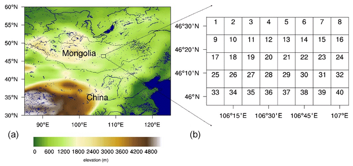
Figure 1The topography and river distribution (a) and the geographical location of the synthetic study area (b).
The soil moisture content and related meteorological and hydrological parameters are monitored by automatic stations maintained by the Coordinated Enhanced Observing Period Asian Monsoon Project (CEOP_ AP) (Bosilovich and Lawford, 2002; Lawford et al., 2004). The CEOP_AP was launched by the World Climate Research Programme (WCRP) to develop an integrated global dataset that can be used to address issues relating to water and energy budget simulations and predictions, monsoon processes, and the prediction of river flows. More details can be found at https://archive.eol.ucar.edu/projects/ceop/dm/insitu/sites/ceop_ap/ (last access: 15 June 2018; Koike, 2004).
2.2 Forcing data
In this study, synthetic experiments were conducted to explore the accuracy of the assimilation schemes. The simulations were driven by forcing data (including radiation, wind, pressure, humidity, precipitation and temperature) from the ERA-Interim dataset (Dee et al., 2011) that had been scaled down to provide a temporal resolution of 1 h.
2.3 Models
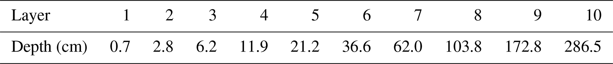
The Common Land Model (CoLM) developed by Dai et al. (2003) is a third-generation land surface model. It combines the best features of three successful models, the Land Surface Model (LSM, Bonan, 1996), the Biosphere-Atmosphere Transfer Scheme (BATS, Dickinson et al., 1993) and the 1994 version of the Chinese Academy of Sciences/Institute of Atmospheric Physics model (IAP94, Dai et al., 2003), and is being further developed. The primary characteristics of the model include 10 unevenly spaced soil layers (see Table 1), 1 vegetation layer, 5 snow layers (depending on the snow depth), explicit treatment of the mass of liquid water, ice and phase changes within the system of the snow and soil, runoff parameterization following the TOPMODEL concept, a tiled treatment of the subgrid fraction of the energy and water budget balance (Dai et al., 2003), and a canopy photosynthesis–conductance mode that describes the simultaneous transfer of CO2 and water vapor into and out of the vegetation. The model parameters include data on the global terrain, elevation, land use, vegetation, land–water mask and hybrid FAO/STATSGO soil types from the USGS, which are available at a resolution of 30 arcsec.
Table 1The node depths (cm) of the 10 soil layers in the CoLM model.
Version 4.0 of the Community Land Model (CLM 4.0) (Lawrence et al., 2011; Oleson et al., 2010) is the land surface parameterization used with the Community Atmosphere Model (CAM 4.0) and the Community Climate System Model (CCSM 4.0). The CLM 4.0 includes bio-geophysics, the hydrologic cycle, biogeochemistry and the dynamic vegetation. CLM 4.0 simulates the bio-geophysical processes in each subgrid unit independently and maintains its own prognostic variables. The parameters used in the CLM4.0 differ from those used in the CoLM. For example, the soil texture data are derived from the IGBP soil data, and the land use data are derived from the UNH Transient Land Use and Land Cover Change Dataset (http://luh.umd.edu/, last access: 15 June 2018).
In addition to using different parameters, the two models have different structures. For example, a model of groundwater–soil-water interactions (Niu et al., 2007; Niu et al., 2005) has been incorporated into the CLM 4.0, while zero water flux at the bottom of a soil column is assumed in the CoLM. Besides, the CLM 4.0 has the same vertical discretization scheme as the CoLM (see Table 1), which makes comparing the results of the two models convenient.
3.1 Forecast and observation systems
Using notation similar to that used by Yilmaz et al. (2011), the forecast system can be written as
where t=1, …, T is the time index, n=1, …, N represents an ensemble member (in this study, the ensemble size is set to 100), is a CoLM forced by the nth perturbed atmospheric forcing, and y is a state vector containing 126 variables. The superscript “f” and “a” specify the forecast and analysis, respectively.
Let x be the state variables related to the water budget, which comprises SM, SIC (the soil moisture content and the soil ice content in percentage at the 10 vertical levels listed in Table 1), CWC and SWE (the canopy's water content and the snow water equivalent in kilograms per square meter, kg m−2). In this study, only x is updated by data assimilation, while the model propagates changes to the other variables over time.
For the traditional EnKF, the forecast error covariance matrix Pt is obtained from the ensemble of their anomalies,
where is the component of related to the water budget, and is the ensemble mean of . To avoid overestimation of the co-variability between shallow observations and soil moisture deeper than a threshold layer s (see Sect. 3.2 for the estimation of s), the following vertical localization function with weighting of observations ρs (Janjić et al., 2011) will be applied on Pt, i.e.,
where l represents for the l-level soil layer, and dl and do represent the depths of l-level soil layer and observation, respectively. |dl−do| is the Euclidian distance between the two layers. μs is estimated by minimizing the following mean square error between vertical localization function Eq. (3) and a step function with threshold layer s,
The estimated μs is listed in Table 2.
Table 2Estimated localization scale factor for different cases.

The observations of the soil moisture content are collected at a depth of 3 cm at 06:00 LT (local time) every day (denoted by ot). The observation system is defined as
where observational operator h is a 22-dimensional vector which linearly interpolates the soil moisture at depths of 2.8 and 6.2 cm to a depth of 3 cm, xt represents the true values of the state variables related to the water budget at the time step t, and εt is the observational error with mean zero and variance Rt. Since the main objective of this study is for methodology related to linear observational operators, choosing the linear interpolation as the observational operator is only for convenience.
3.2 Assimilation with water budget constraint
Assimilating data on the soil moisture content usually results in an imbalance in the water budget. To reduce this imbalance, a weak constraint on the water budget (Yilmaz et al., 2011) is adopted in this study. The ensemble water budget residual at time step t can be expressed as
where
where c is a 22-dimensional vector that converts the units to millimeters (mm) and adds up the states in x, and the diagnostic variables Prt, Ev and Rn (mm) are scalars specifying the states of the precipitation, evapotranspiration and runoff, respectively, in each pixel.
The cost function used to estimate the state variables with the weak water budget constraint (Eq. 6) is
where
is an estimate of the variance of βn,t, and Ps,t represents a forecast error covariance matrix defined by
where Pt is defined as Eq. (2); [ρs] is a diagonal matrix which localizes the soil moisture error (i.e., it is ρs defined by Eq. (3) for the soil moisture contents and 1 for other variables). is also a diagonal matrix which inflates the forecast soil moisture error (i.e., it is a scalar λt for the soil moisture contents and 1 for other variables). λt is estimated by minimizing −2 times the log-likelihood function of the difference between the forecast and the observation (Dee and Da Silva, 1999; Liang et al., 2012; Zheng, 2009),
The estimated forecast error inflation factor is denoted as . The perturbed analysis states of the variables related to water budget can be derived by minimizing Eq. (8), which has the analytic form
where εn,t is generated from a normal distribution with mean zero and variance Rt, and
its analysis error covariance matrix.
To estimate the optimal threshold layer, define −2 times the log-likelihood function of the total difference between the forecasts and the observations,
The optimal threshold layer is selected as the smallest number s such that Ls is the minimum of . The final analysis state is the selected corresponding to the optimal threshold layer . The complete assimilation procedure with water budget constraint is shown in Fig. 2.
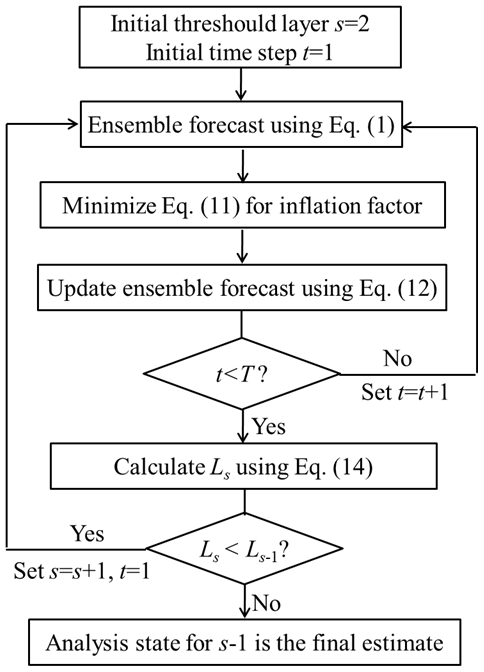
Figure 2The assimilation procedure and localization scale factor estimation in the experiments. All of the equations are in accordance with that described in the text.
3.3 Bias-aware assimilation
The bias-aware data assimilation proposed by Dee (2005) is adopted to correct the analysis bias.
Let bt be the estimated bias at time step t and set b1=0. For t>1,
where the scalar parameter γ that controls the magnitude of the forecast bias is estimated following Dee and Todling (2000) (see Eqs. A5–A6 of Appendix A), is the ensemble mean of the perturbed forecast states from the analysis state , and is the corresponding adjusted forecast error covariance (see Eq. A2 of Appendix A).
Then the perturbed assimilated states are
where and are defined by Eqs. (A7)–(A9) in Appendix A, respectively.
4.1 Experimental design
To investigate the performance of the WCEnKF-based methods that incorporate inflation, vertical local localization and bias-aware assimilation, synthetic experiments were performed using the CoLM. Unlike the “perfect model” assumption used in Yilmaz et al. (2011), the assumptions of this study account for the error in the model, especially the structural error. Because there were structural differences in the models of the water cycle (see Sect. 2.3) used in the two models, CLM 4.0 was used to generate the “true values” (i.e., to perform a reference run) for the synthetic experiments and CoLM was selected as the forecast operator (i.e., to perform an open-loop run). Therefore, the CLM 4.0 and the CoLM were both integrated on a 0.125∘ grid (see Fig. 1 for the locations) with a time step of 1 h. The assimilation time was set to 06:00 LT every day. The assimilation experiments were conducted with five scenarios: the traditional ensemble Kalman filter (EnKF), a weakly constrained ensemble Kalman filter (WCEnKF), a weakly constrained ensemble Kalman filter with inflation (WCEnKF-Inf), a weakly constrained ensemble Kalman filter with inflation and localization (WCEnKF-Inf-Loc), and a weakly constrained ensemble Kalman filter with inflation, localization and bias-aware assimilation (WCEnKF-Inf-Loc-BA).
Synthetic observations were obtained by interpolating to a depth of 3 cm and adding noise with a normal distribution ( %)). The initial state x0 was generated by running the CoLM from 1 October 2002 to 1 June 2003. Each component of the initial state was perturbed using an independent standard Gaussian random variable times 5 % of magnitude of the component. The forcing data were perturbed in the manner described in Yilmaz et al. (2011). The synthetic experiments were conducted from 1 June to 1 October 2003. The state variables for each pixel were updated independently.
4.2 Validation statistics
4.2.1 Model error and bias
The model errors are defined as the difference between the actual values and the model's predictions based on true initial values, and the bias is the average of the error in the model during the relevant period. Let xt denote the true values of the soil moisture content at time t for a location and vertical soil layer. denotes the model-predicted soil moisture from the true state at the previous time step t−1. The model's bias and error variance for one step can be written as
where ats is the number of time steps over which the observations made at 06:00 LT each day are assimilated.
4.2.2 Validation of analysis soil moisture
The true soil moisture content values from 07:00 to 05:00 LT the next day are used to validate analysis states. For a location and vertical soil layer, let xt,h be the true soil moisture content at hour h on day t, and let represent the forecasted soil moisture content at hour h from analysis state at 06:00 LT on day t. The analysis bias is defined as
The analysis error variance is defined as
(See Appendix B for the proof.)
4.2.3 Water balance
Following Yilmaz (2011), the water budget imbalance at the location is evaluated using the water balance residual,
where N is the ensemble size, ats is the number of assimilation time steps, and rn,t is the ensemble water budget residual at time step t as defined in Eq. (6).
In the synthetic experiments, the magnitudes of the model's bias and error were calculated using Eqs. (17) and (18), respectively, and are shown in Fig. 3. It shows that the model's bias was almost negative from Fig. 3a. The negative bias in the surface layer was the result of a combination of a lower surface roughness and a larger leaf area index in the CoLM; these values led to more soil evaporation and more canopy interception and could result in a smaller amount of water infiltrating the soil than the amount modeled using the CLM 4.0. In the CoLM, the porosity of each layer was less than it was in the CLM 4.0, which retained less water and contributed to the negative bias of the upper nine layers. However, the magnitude of the bias increased to 2 % in the bottom layer. The significant difference between the two models at the bottom layer could be ascribed to their different boundary conditions. Interactions between the soil moisture content and the ground water at the bottom of the soil column were modeled in the CLM 4.0 (Oleson et al., 2010) but not in the CoLM. The error in each model (Fig. 3b) fluctuated in a manner similar to that of the model's bias. Unbiased observations are necessary for correcting bias in a model, which is not possible in many realistic applications, especially in assimilating remote sensing retrievals. Since satellite observations of the soil moisture content of deep layers are unavailable, only removing the bias in shallow layers would introduce error in model dynamics.
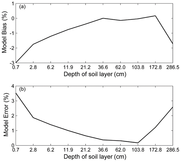
Figure 3The areal average of the model's bias (a) and error (b) for one step in the soil moisture content between the CoLM and the CLM 4.0. The horizontal axis represents the layer depth.
5.1 Forecast error inflation and vertical localization
In the synthetic experiments, the study domain comprised 40 pixels. At each point in the grid-scale threshold layer, the localization scale factor μs was determined independently. Therefore, in total nine sets of experiments with different localization scale factors (see Table 2) were conducted separately. Among these experiments, the “optimal” case for each pixel was defined as the case in which the column- averaged analysis error (Eq. 20) was minimized (shown in Fig. 4). According to Fig. 4a, the corresponding threshold layer s of μs was generally between 5 and 6 in both cases, which could be ascribed to the homogeneous soil texture and land cover. In the WCEnKF-Inf-Loc, there were 19 pixels in which the threshold layers were “optimal,” and the layers selected in the other pixels were suboptimal (most were roughly one layer away from the “optimal” case). As shown in Fig. 4b, the spatial average of the root analysis error variance (Eq. 20) of the WCEnKF-Inf-Loc (4.09 %) was comparable with the optimal value (3.84 %) even though s was not selected on the basis of minimizing the analysis error.
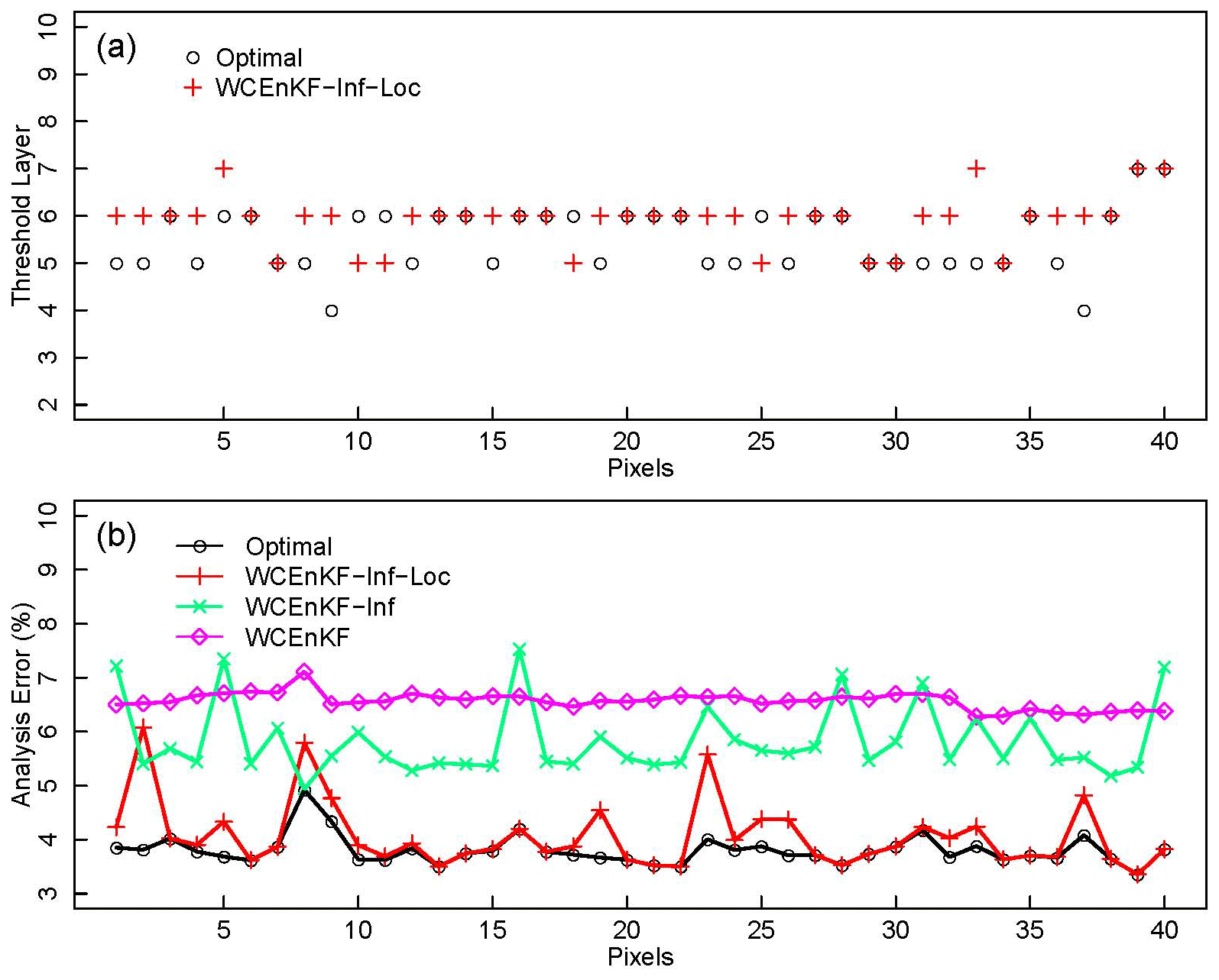
Figure 4The threshold layers and analysis error for each pixel in the synthetic experiment. Graph (a) illustrates the optimal and WCEnKF-Inf-Loc threshold layers of each pixel. Graph (b) shows the column RSME of each pixel in different schemes with water balance constraint (Optimal, WCEnKF-Inf-Loc, WCEnKF-Inf and WCEnKF). The horizontal axes of (a) and (b) represent the 40 pixels in the study domain.
The spatial average of the root analysis error variance in each layer in the schemes with (WCEnKF-Inf-Loc and WCEnKF-Inf) and without (WCEnKF) inflation are displayed in Fig. 5a. Above 36.6 cm, the analysis errors of the schemes without inflation (6.70 %) were substantially larger than those of the schemes with inflation (2.00 %) for the synthetic experiments. This suggested that inflation provided a better estimate in the layers close to the observation. When no inflation was performed, the accuracy of the soil moisture content was barely improved over that of the open loop (not shown here).
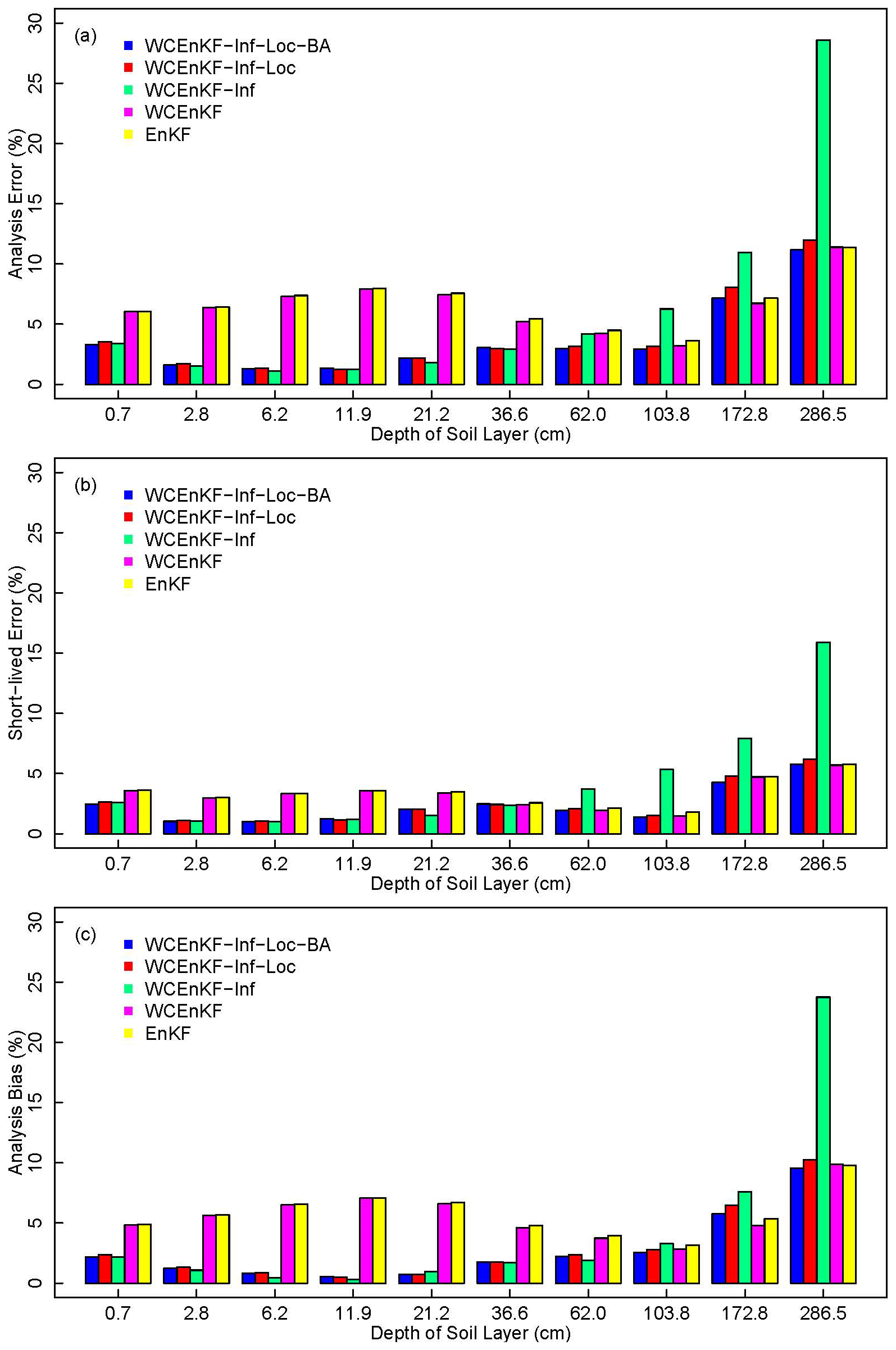
Figure 5The assimilation results in each layer for the five schemes: a weakly constrained bias-aware ensemble Kalman filter with forecast error inflation and vertical localization (WCEnKF-Inf-Loc-BA), a weakly constrained ensemble Kalman filter with forecast error inflation and vertical localization (WCEnKF-Inf-Loc), a weakly constrained ensemble Kalman filter with forecast error inflation (WCEnKF-Inf), a weakly constrained ensemble Kalman filter (WCEnKF), and the traditional assimilation (EnKF). Graphic (a) is for spatial averaged analysis error of the soil moisture content, (b) is for the short-lived error and (c) is for the analysis bias.
By comparing the schemes with (WCEnKF-Inf-Loc) and without (WCEnKF-Inf) vertical localization, the impact of this approach on the assimilation accuracy in each layer is shown in Fig. 5a. Because the threshold layer of the localization function ρs was layer 6 (36.6 cm) for 28 of the pixels (see Fig. 4a), the spatial average of root analysis error variance of the results of the WCEnKF-Inf-Loc is almost identical to that of the results of the WCEnKF-Inf for depths above 36.6 cm. In contrast, inflation increased the analysis error in the soil moisture content of the deep layers in the WCEnKF-Inf from 6.38 % to 12.49 %. In this model, the sample error covariances of the moisture contents of shallow and deep soil were inflated by a factor greater than 6 (the average inflation factor was 6.25). This could lead to larger assimilation errors for deep soil moisture profiles in the WCEnKF-Inf. Therefore, inflation should be used with vertical localization to reduce the spurious covariance resulting from the covariance inflation-based approach.
As it was in the synthetic experiments, vertical localization (WCEnKF-Inf-Loc) was helpful in avoiding erroneous estimates of the soil moisture contents at lower levels (in the WCEnKF-Inf). A comparison of the analysis error at a depth of 3 cm (i.e., the depth of the assimilated observations was 3 cm) in the models with (WCEnKF-Inf and WCEnKF-Inf-Loc) and without (WCEnKF) inflation showed that the inflation technique significantly reduces the analysis error at the depth at which observations are made.
To investigate the role of bias correction, the spatial averaged root analysis error variances (Eq. 20) of WCEnKF-Inf-Loc-BA and WCEnKF-Inf-Loc were compared. According to Fig. 5a, the spatial averaged root analysis error variances of the two schemes were comparable with each other (2.12 % for the WCEnKF-Inf-Loc-BA and 2.16 % for the WCEnKF-Inf-Loc) in the layers that were shallower than 36.6 cm. This could be due to the observations being closer to the shallow layers and the vertical localization approach being reasonably effective at reducing the bias. However, for the layers that were deeper than 62.0 cm, the averaged root analysis error of the WCEnKF-Inf-Loc-BA (6.05 %) was less than that of the WCEnKF-Inf-Loc (6.59 %).
5.2 The water budget constraint
In the synthetic experiment, the weak constraint on the water budget reduced the water balance residual significantly in each pixel and the results are shown in Fig. 6. It shows that the spatial average of the water balance residual of the WCEnKF scheme was 0.0487 mm, which was much smaller than that of the EnKF scheme (0.1389 mm). Therefore, the assimilation scheme with a water budget constraint can indeed reduce the water balance residuals relative to the assimilation scheme without a water budget constraint, which is consistent with the results of previous studies (Yilmaz et al., 2011; Yilmaz et al., 2012). The interquartile range of the water balance residuals in the 40 pixels for the WCEnKF scheme was 0.0042 mm, which was less than half of that for the EnKF scheme (0.0098 mm). The reduced spread of the water balance residuals signals a more stable water balance budget with the water budget constraint.
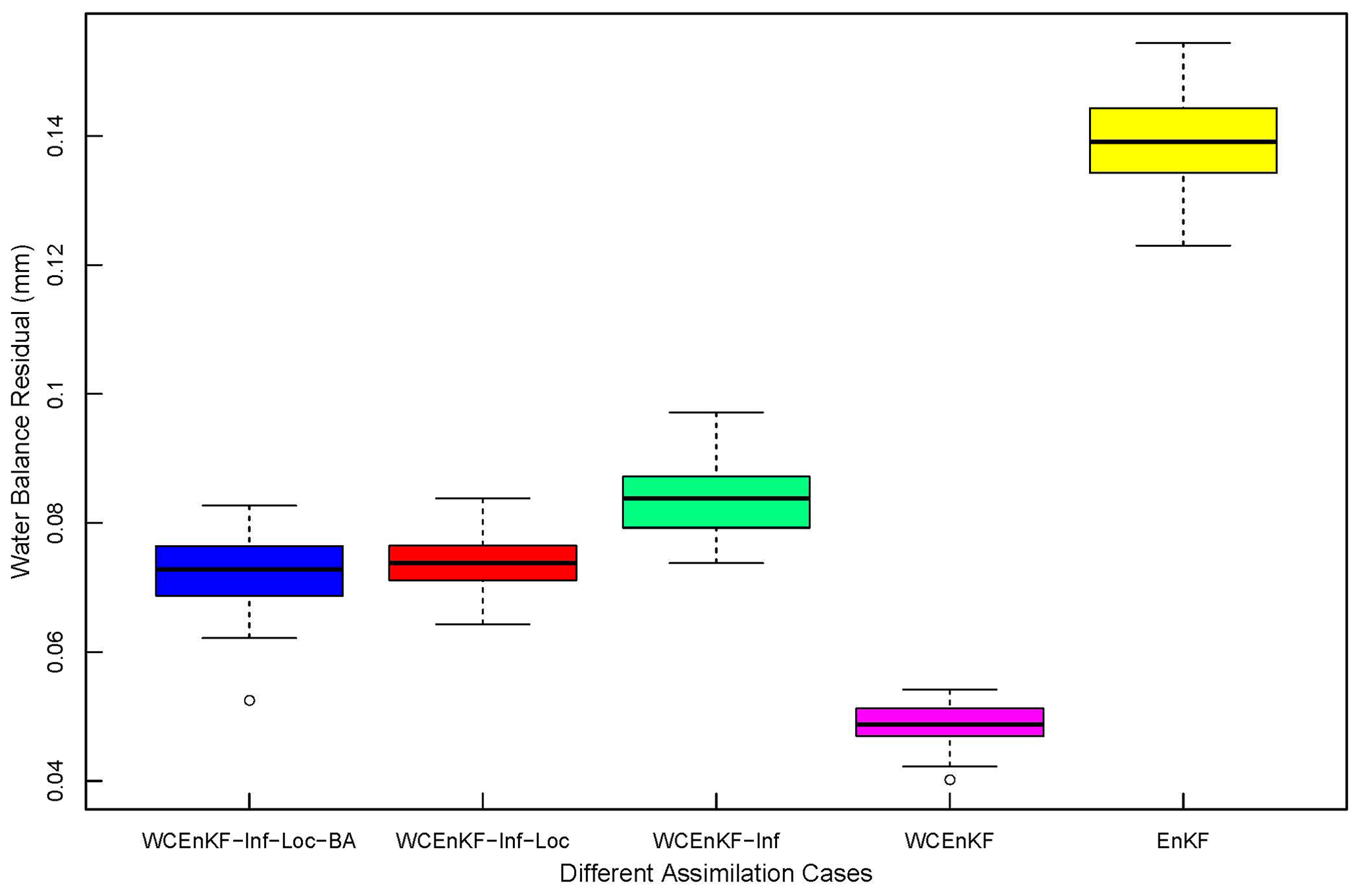
Figure 6The box plot of the water balance residual in all 40 pixels for the WCEnKF-Inf-Loc-BA, WCEnKF-Inf-Loc,WCEnKF-Inf, WCEnKF and EnKF assimilation schemes.
The spatial averages of the water balance residual for WCEnKF-Inf, WCEnKF-Inf-Loc and WCEnKF-Inf-Loc-BA were 0.0834, 0.0737 and 0.0723 mm, respectively. The corresponding interquartile range was 0.0079, 0.0051 and 0.0072 mm, respectively. They are still much smaller than those for the EnKF scheme, despite a greater increase compared to WCEnKF. This demonstrates the weak water budget constraint is still effective in reducing the magnitude and spread of the water imbalance, despite the association of more complicated assimilation approaches.
6.1 Covariance inflation and vertical localization
In this study, the cost function used to estimate the state variables with the weak water budget constraint (Eq. 8) consists of three parts, which are related with observations, model forecasts and water residuals (Yilmaz et al., 2012). It is represented as a summation of three scalars, no matter how many observations are assimilated. Therefore, inflating one scalar (e.g., model forecasts) seems to have a similar impact to deflating another one (e.g., water residual), and in particular the weights associated with this problem can be shown as a function of the ratio of these three scalars. Specifically, inflation of forecast error covariance has a somewhat similar impact to deflation of the water balance residual covariance. If the focus of a study or experiment is reducing water balance, WCEnKF could be a better choice and computationally faster than the WCEnKF-Inf and WCEnKF-Inf-Loc schemes. Accordingly, it is plainly obvious that the water balance residual of the WCEnKF-Inf scheme is larger than that of the WCEnKF scheme. However, the objective in this study is to reduce water balance without significantly increasing the analysis error. Since the analysis errors for WCEnKF in the layers shallower than 36.6 cm are significantly larger than those for the schemes with inflation, WCEnKF is not preferred.
According to Fig. 5a, the covariance inflation improved the estimates of the soil moisture content in the shallow layers independently of whether vertical localization was used. This is primarily because the observation operator, h, is the linear operator that was used to interpolate the soil moisture content at depths of 2.8 and 6.2 cm to a depth of 3 cm. Then, the likelihood function for the inflation factor (Eq. 11) depends only on the observations and predictions of the soil moisture content in the second and third layers. The mean value of the inflation factor is 6.25 for WCEnKF-Inf, indicating that the initial forecast spread is not large enough. This leads to an improvement in the forecast error statistics in the shallow layers, and to further improvements in the assimilated soil moisture contents of those layers.
However, the soil moisture contents of the deep layers are not directly related to the inflation factor. Inflating the forecast errors in the deep layers leads to an overestimation of the corresponding forecast error covariance and could lead to larger analysis errors in the deep layers (see WCEnKF-Inf in Fig. 5a). Therefore, in this study, the vertical localization approach was developed to prevent soil moisture over-fitting for deep layers. Using all observations for threshold s is only for model selection (from the 10 layers), not for fitting parameters. When vertical localization is used, the soil moisture contents of the deep layers are not significantly updated. Consequently, larger errors are avoided in the deep layers (see WCEnKF-Inf-Loc in Fig. 5a).
Compared to traditional EnKF without inflation and localization, although mainly the soil moisture contents of layers above the threshold layer (usually the fifth or sixth layer) were updated at each time step during the assimilation process when the WCEnKF-Inf-Loc was used, Fig. 5a shows that the soil moisture contents of the layers below the threshold layer, especially the sixth and seventh layers, are also improved. This may be because the model propagates changes in the shallow layers downward, adjusting the soil moisture contents of the deep layers. Because the soil moisture content of layers above the threshold layer was improved during the previous time step, this process results in better predictions of the soil moisture contents of layers below the threshold layer and, therefore, reduces the analysis error in layers below the threshold layer.
6.2 Bias correction
Geophysical models are never perfect and usually produce estimates with biases that vary in time and in space (Reichle, 2008). Therefore, bias correction is important for assimilating data into models. In this study, only soil moisture in shallow layers can be observed (in order to mimic the satellite observation), so the bias for the soil moisture in deeper layers cannot be entirely removed using only the observations. However, bias can be detected by monitoring statistics of observation-minus-forecast residuals in the assimilation systems. Therefore the bias-aware assimilation proposed by Dee (2005) was further applied to reduce the bias of soil moisture in all layers.
For further evaluating the efficacy of the bias-aware assimilation scheme, the analysis error variance was decomposed to a short-lived component (Fig. 5b) and a bias component (Fig. 5c) for the synthetic experiment. It shows that for the bias-blind data assimilation scheme (WCEnKF-Inf-Loc), both short-lived errors and biases are reduced in the layers close to observation, while maintaining similar levels to those for EnKF for the deeper layers. The covariance inflation can play an important role in bias reduction. Bias can only be seen during long assimilation periods. At an instant time, bias and error are mixed. For the traditional EnKF, the forecast error covariance matrix obtained from the ensemble of their anomalies (Eq. 2) mainly represents short-lived error, so it has to be inflated to include error related to bias. Moreover, the bias could be further reduced by the additional bias-aware assimilation.
There are other bias estimation approaches in data assimilation, for example, treading bias as model variables and estimate in assimilation (De Lannoy et al., 2007; Dee and Da Silva, 1998), adjusting the state variable of the forecast model (not only their covariance matrix) in each forecast step (Zhang et al., 2014, 2015), and addressing the biases in the model and observations by rescaling their cumulative distribution functions (Koster et al., 2009; Reichle and Koster, 2004). The scheme proposed here can provide a baseline to validate the efficacy of these approaches and could be further improved after these bias corrections.
6.3 Broader implications
In our schemes, the canopy's water content was directly updated by the soil moisture observations, following the approach of previous studies (Yilmaz et al., 2011; Yilmaz et al., 2012). The canopy's water content (CWC) and snow water equivalent (SWE) are related to the water budget. If the water budget constraint is absent, they are normally not updated, and the vegetation module transports the water into the vegetation layer. However, the present study focused on the assimilation with the water budget constraint, so updating CWC and SWE would help to reduce the water budget residuals.
For the assimilation with the water budget constraint but without updates of CWC and SWE, the state variables related to the water budget are decomposed as , where 1x comprises SM and SIC, and 2x comprises CWC and SWE. converts the units of to millimeters (mm). The assimilation for the non-updated 2x can be achieved by substituting x and βn,t in Sect. 3.2 with 1x and 1βn,t, respectively, that is
where Prt, Ev and Rn are diagnostic variables specifying the states of the precipitation, evapotranspiration and runoff, respectively. In this way, the canopy's water content are not updated and the vegetation module transports the water into the vegetation layer. In this study, the range of the estimated CWCs for all assimilations with or without an update of 2x is only about 0.005 mm. Considering the estimated water budget residuals are between 0.05 mm and 0.14 mm and there is no SWE in the summer period, we conclude that an update of CWC has a little impact on water balance in this study.
The highest computational cost in the assimilation system is computing the localization function at each model grid cell. For the synthetic experiments with the CoLM model and 40 grids, it takes about 24 h runtime on the personal workstation. For global data assimilation with 2∘ resolution it could take about 3 months. However, the super-server and parallel computation can significantly shorten the computational time. A regional scale using soil texture or climate regimes can also be used to delineate different regions. In this way, the computational time of global data assimilation can be further reduced.
In the near future, we plan to validate the major conclusions under different soil conditions and land cover types. Vertical localization, which uses adjacent observations, should also be tested in future work. More detailed analyses of the bias correction for assimilating remote sensing retrievals should be performed. The response of the analytic soil moisture content to weather predictions also needs to be investigated. Completing these studies should improve the state of research into land-atmosphere interactions.
In this study, observations of the soil moisture content at a depth of 3 cm were assimilated using an ensemble Kalman filter with several improvements. Firstly, an adaptive forecast error inflation based on maximum-likelihood estimation was adopted to reduce the analysis error. This study supports the idea that the proper form of the forecast error covariance matrix is crucial for reducing the analysis error near the layers in which observations are made. Secondly, an adequate vertical localization for the ensemble-based filter was proposed, associated with the forecast error covariance inflation, to avoid misestimates of the soil moisture contents of deep layers. Lastly, a constraint on the water balance was used in this study to reduce the water budget residual substantially without significantly changing the assimilation accuracy. The experiment results of synthetic study show that the WCEnKF-Inf-Loc assimilation scheme can reduce the analysis error from 6.70 % to 2.00 % in the shallow layers, with both the short-lived analysis error and the analysis bias reduced. It also leads to a rational water budget residual with spatial average 0.0737 mm, which is much smaller than 0.1389 mm of the EnKF scheme. The bias-aware assimilation scheme is potentially useful to further reduce the analysis error arising from model bias.
For correcting the bias of the analysis states in Eq. (12), the bias-aware assimilation (Dee, 2005) is applied.
Let bt is the forecast bias at time step t, and set b1=0. Then
where is the ensemble mean of the perturbed forecast states predicted from the perturbed analysis state at previous time step , the forecast error covariance matrix is in the form
where the localization threshold s is adopted from the bias-blind scheme documented in Sect. 3.2,
and the inflation factor is estimated by minimizing
The scalar parameter γ in Eq. (A1) that controls the magnitude of the forecast bias estimates, is derived by
where μ is estimated by minimizing the following objective function (Dee and Todling, 2000)
Then the perturbed analysis states is calculated as
where
and
For a location and vertical soil layer, the analysis error variance in the synthetic experiment is defined as
From the definition of analysis bias (Eq. 19), the last term on the right hand side of is zero, so Eq. (21) is proved.
The soil moisture observations are available at https://archive.eol.ucar.edu/projects/ceop/dm/insitu/sites/ceop_ap/ (Koike, 2004). The ERA-Interim forcing data used in the synthetic experiments are obtained from https://apps.ecmwf.int/datasets/data/interim-full-daily/levtype=sfc/ (last access: 15 June 2018, Dee et al., 2011).
BD performed the simulations and assimilations. XZ and GW designed the research. GW analyzed the results. TL collected and preprocessed the data. GW and XZ prepared the paper with contributions from all co-authors.
The authors declare that they have no conflict of interest.
We would like to thank the Editor and three anonymous reviewers for their insightful comments, which improved the paper. We also thank Yongjiu Dai and Qingyun Duan for their help in land surface model.
This study research has been supported by the National Key R&D Program of China (grant nos. 2019YFC1510002, 2015CB953703) and the National Natural Science Foundation of China (grant nos. 41930970, 42077421, 41705086).
This paper was edited by Shraddhanand Shukla and reviewed by three anonymous referees.
Anderson, J. L. and Anderson, S. L.: A Monte Carlo implementation of the nonlinear fltering problem to produce ensemble assimilations and forecasts, Mon. Weather Rev., 127, 2741–2758, 1999.
Bartalis, Z., Wagner, W., Naeimi, V., Hasenauer, S., Scipal, K., Bonekamp, H., Figa, J., and Anderson, C.: Initial soil moisture retrievals from the METOP-A Advanced Scatterometer (ASCAT). Geophys. Res. Lett., 34, L20401, https://doi.org/10.1029/2007gl031088, 2007.
Bauser, H. H., Berg, D., Klein, O., and Roth, K.: Inflation method for ensemble Kalman filter in soil hydrology, Hydrol. Earth Syst. Sci., 22, 4921–4934, https://doi.org/10.5194/hess-22-4921-2018, 2018.
Bonan, G. B.: Land surface model (LSM version 1.0) for ecological, hydrological, and atmospheric studies: Technical description and users guide. Technical note, National Center for Atmospheric Research, Boulder, CO (United States), Climate and Global Dynamics Div., 1996.
Bosilovich, M. G. and Lawford, R.: Coordinated enhanced observing period (CEOP) international workshop, B. Am. Meteorol. Soc., 83, 1495–1499, 2002.
Chen, F., Crow, W. T., and Ryu, D.: Dual Forcing and State Correction via Soil Moisture Assimilation for Improved Rainfall-Runoff Modeling, J. Hydrometeorol., 15, 1832–1848, 2014.
Constantinescu, E. M., Sandu, A., Chai, T., and Carmichael, G. R.: Ensemble-based chemical data assimilation I: general approach, Q. J. Roy. Meteor. Soc., 133, 1229–1243, 2007.
Crow, W. T. and Loon, E. V.: Impact of incorrect model error assumptions on the sequential assimilation of remotely sensed surface soil moisture. J. Hydrometeorol., 7, 421–432, 2006.
Crow, W. T. and Wood, E. F.: The assimilation of remotely sensed soil brightness temperature imagery into a land surface model using Ensemble Kalman filtering: a case study based on ESTAR measurements during SGP97, Adv. Water Resour., 26, 137–149, 2003.
Crow, W. T., Chen, F., Reichle, R. H., and Liu, Q.: L band microwave remote sensing and land data assimilation improve the representation of prestorm soil moisture conditions for hydrologic forecasting, Geophys. Res. Lett., 44, 5495–5503, 2017.
Dai, Y., Zeng, X., Dickinson, R. E., Baker, I., Bonan, G. B., Bosilovich, M. G., Denning, A. S., Dirmeyer, P. A., Houser, P. R., Niu, G., Oleson, K. W., Schlosser, C. A., and Yang, Z.-L.: The Common Land Model, B. Am. Meteorol. Soc., 84, 1013–1023, 2003.
Dee, D. P.: Bias and data assimilation, Q. J. Roy. Meteoro. Soc., 131, 3323–3343, 2005.
Dee, D. P. and Da Silva, A. M.: Data assimilation in the presence of forecast bias, Q. J. Roy. Meteor. Soc., 124, 269–295, 1998.
Dee, D. P. and Da Silva, A.M.: Maximum-likelihood estimation of forecast and observation error covariance parameters. Part I: Methodology, Mon. Weather Rev., 127, 1822–1834, 1999.
Dee, D. P. and Todling, R.: Data assimilation in the presence of forecast bias: The GEOS moisture analysis, Mon. Weather Rev., 128, 3268–3282, 2000.
Dee, D. P., Gaspari, G., Redder, C., Rukhovets, L., and Da Silva, A. M.: Maximum-likelihood estimation of forecast and observation error covariance parameters. Part II: Applications, Mon. Weather Rev., 127, 1835–1849, 1999.
Dee, D. P., Uppala, S. M., Simmons, A. J., Berrisford, P., Poli, P., Kobayashi, S., Andrae, U., Balmaseda, M. A., Balsamo, G., Bauer, P., Bechtold, P., Beljaars, A. C. M., van de Berg, L., Bidlot, J., Bormann, N., Delsol, C., Dragani, R., Fuentes, M., Geer, A. J., Haimberger, L., Healy, S. B., Hersbach, H., Hólm, E. V., Isaksen, L., Kållberg, P., Köhler, M., Matricardi, M., McNally, A. P., Monge-Sanz, B. M., Morcrette, J. J., Park, B. K., Peubey, C., de Rosnay, P., Tavolato, C., Thépaut, J. N., and Vitart, F.: The ERA-Interim reanalysis: configuration and performance of the data assimilation system, Q. J. Roy. Meteor. Soc., 137, 553–597, 2011.
De Lannoy, G. J. M., Reichle, R. H., Houser, P. R., Pauwels, V. R. N., and Verhoest, N. E. C.: Correcting for forecast bias in soil moisture assimilation with the ensemble Kalman filter. Water Resour. Res., 43, W10799, https://doi.org/10.1029/2007WR006542, 2007.
Delworth, T. L. and Manabe, S.: The influence of potential evaporation on the variabilities of simulated soil wetness and climate, J. Climate, 1, 523–547, 1988.
Dickinson, R. E., Henderson-Sellers, A., and Kennedy, P. J.: Biosphere Atmosphere Transfer Scheme (BATS) Version le as Coupled to the NCAR Community Climate Model, NCAR Tech. Note NCAR/TN-378+STR, 72 pp., 1993.
Dorigo, W. A., Wagner, W., Hohensinn, R., Hahn, S., Paulik, C., Xaver, A., Gruber, A., Drusch, M., Mecklenburg, S., van Oevelen, P., Robock, A., and Jackson, T.: The International Soil Moisture Network: a data hosting facility for global in situ soil moisture measurements, Hydrol. Earth Syst. Sci., 15, 1675–1698, https://doi.org/10.5194/hess-15-1675-2011, 2011.
Dumedah, G. and Walker, J. P.: Evaluation of Model Parameter Convergence when Using Data Assimilation for Soil Moisture Estimation, J. Hydrometeorol., 15, 359–375, 2014.
El Gharamti, M., Raeder, K., Anderson, J., and Wang, X.G.: Comparing Adaptive Prior and Posterior Inflation for Ensemble Filters Using an Atmospheric General Circulation Model, Mon. Weather Rev., 147, 2535–2553, 2019.
Entekhabi, D., Njoku, E. G., O'Neill, P. E., Kellogg, K. H., Crow, W. T., Edelstein, W. N., Entin, J. K., Goodman, S. D., Jackson, T. J., and Johnson, J.: The soil moisture active passive (SMAP) mission, P. IEEE, 98, 704–716, 2010.
Evensen, G.: Sequential data assimilation with a nonlinear quasi-geostrophic model using Monte Carlo methods to forecast error statistics, J. Geophys. Res., 99, 10143–10162, 1994.
Gruber, A., Crow, W. T., and Dorigo, W. A.: Assimilation of Spatially Sparse In Situ Soil Moisture Networks into a Continuous Model Domain, Water Resour. Res., 54, 1353–1367, 2018.
Gusev, Y. and Novak, V.: Soil water–main water resources for terrestrial ecosystems of the biosphere, J. Hydrol. Hydromech., 55, 3–15, 2007.
Han, E., Crow, W. T., Holmes, T., and Bolten, J.: Benchmarking a Soil Moisture Data Assimilation System for Agricultural Drought Monitoring, J. Hydrometeorol., 15, 1117–1134, 2014.
Janjić, T., Nerger, L., Albertella, A., Schröter, J., and Skachko, S.: On Domain Localization in Ensemble-Based Kalman Filter Algorithms, Mon. Weather Rev., 139, 2046–2060, 2011.
Kerr, Y. H., Waldteufel, P., Wigneron, J.-P., Delwart, S., Cabot, F., Boutin, J., Escorihuela, M.-J., Font, J., Reul, N., and Gruhier, C.: The SMOS mission: New tool for monitoring key elements ofthe global water cycle, P. IEEE, 98, 666–687, 2010.
Koike, T.: Coordinated Enhanced Observing Period (CEOP) – an initial step for integrated global water cycle observation, World Meteorological Organization Bulletin, 53, 115–121, 2004.
Koster, R. D., Guo, Z. C., Yang, R. Q., Dirmeyer, P. A., Mitchell, K., and Puma, M. J.: On the Nature of Soil Moisture in Land Surface Models, J. Climate, 22, 4322-4335, 2009.
Kumar, S. V., Peters-Lidard, C. D., Mocko, D., Reichle, R., Liu, Y. Q., Arsenault, K. R., Xia, Y. L., Ek, M., Riggs, G., Livneh, B., and Cosh, M.: Assimilation of Remotely Sensed Soil Moisture and Snow Depth Retrievals for Drought Estimation, J. Hydrometeorol., 15, 2446–2469, 2014.
Lawford, R., Stewart, R., Roads, J., Isemer, H., Manton, M., Marengo, J., Yasunari, T., Benedict, S., Koike, T., and Williams, S.: Advancing global-and continental-scale hydrometeorology: Contributions of GEWEX hydrometeorology panel, B. Am. Meteorol. Soc., 85, 1917–1930, 2004.
Lawrence, D. M., Oleson, K. W., Flanner, M. G., Thornton, P. E., Swenson, S. C., Lawrence, P. J., Zeng, X., Yang, Z.-L., Levis, S., Sakaguchi, K., Bonan, G. B., and Slater, A. G.: Parameterization improvements and functional and structural advances in Version 4 of the Community Land Model, J. Adv. Model. Earth Sy., 3, M03001, https://doi.org/10.1029/2011ms000045, 2011.
Li, B., Toll, D., Zhan, X., and Cosgrove, B.: Improving estimated soil moisture fields through assimilation of AMSR-E soil moisture retrievals with an ensemble Kalman filter and a mass conservation constraint, Hydrol. Earth Syst. Sci., 16, 105–119, https://doi.org/10.5194/hess-16-105-2012, 2012.
Liang, X., Zheng, X., Zhang, S., Wu, G., Dai, Y., and Li, Y.: Maximum likelihood estimation of inflation factors on error covariance matrices for ensemble Kalman filter assimilation, Q. J. Roy. Meteor. Soc., 138, 263–273, 2012.
Loizu, J., Massari, C., Alvarez-Mozos, J., Tarpanelli, A., Brocca, L., and Casali, J.: On the assimilation set-up of ASCAT soil moisture data for improving streamflow catchment simulation, Adv. Water Resour., 111, 86–104, 2018.
Lu, H., Koike, T., Yang, K., Hu, Z. Y., Xu, X. D., Rasmy, M., Kuria, D., and Tamagawa, K.: Improving land surface soil moisture and energy flux simulations over the Tibetan plateau by the assimilation of the microwave remote sensing data and the GCM output into a land surface model. Int. J. Appl. Earth Obs., 17, 43–54, 2012.
Lu, H., Yang, K., Koike, T., Zhao, L., and Qin, J.: An Improvement of the Radiative Transfer Model Component of a Land Data Assimilation System and Its Validation on Different Land Characteristics, Remote Sensing, 7, 6358–6379, 2015.
McColl, K. A., He, Q., Lu, H., and Entekhabi, D.: Short-Term and Long-Term Surface Soil Moisture Memory Time Scales Are Spatially Anticorrelated at Global Scales, J. Hydrometeorol., 20, 1165–1182, 2019.
Miyoshi, T.: The Gaussian approach to adaptive covariance inflation and its implementation with the local ensemble transform Kalman filter, Mon. Weather Rev., 139, 1519–1534, 2011.
Miyoshi, T., Kalnay, E., and Li, H.: Estimating and including observation-error correlations in data assimilation, Inverse Prob. Eng., 32, 1–12, 2012.
Niu, G. Y., Yang, Z. L., Dickinson, R. E., and Gulden, L. E.: A simple TOPMODEL-based runoff parameterization (SIMTOP) for use in global climate models, J. Geophys. Res.-Atmos., 110, D21106, https://doi.org/10.1029/2005JD006111, 2005.
Niu, G.-Y., Yang, Z.-L., Dickinson, R. E., Gulden, L. E., and Su, H.: Development of a simple groundwater model for use in climate models and evaluation with Gravity Recovery and Climate Experiment data, J. Geophys. Res., 112, D07103, https://doi.org/10.1029/2006jd007522, 2007.
Njoku, E. G., Jackson, T. J., Lakshmi, V., Chan, T. K., and Nghiem, S. V.: Soil moisture retrieval from AMSR-E, IEEE T. Geosci. Remote, 41, 215–229, 2003.
Oleson, K. W., Lawrence, D. M., Gordon, B., Flanner, M. G., Kluzek, E., Peter, J., Levis, S., Swenson, S. C., Thornton, E., and Feddema, J.: Technical description of version 4.0 of the Community Land Model (CLM), NCAR Tech. Note NCAR/TN-478+STR, 257 pp., 2010.
Pan, M. and Wood, E. F.: Data assimilation for estimating the terrestrial water budget using a constrained ensemble Kalman filter, J. Hydrometeorol., 7, 534–547, 2006.
Pielke, R. A.: Influence of the spatial distribution of vegetation and soils on the prediction of cumulus Convective rainfall, Rev. Geophys., 39, 151–177, 2001.
Pinnington, E., Quaife, T., and Black, E.: Impact of remotely sensed soil moisture and precipitation on soil moisture prediction in a data assimilation system with the JULES land surface model, Hydrol. Earth Syst. Sci., 22, 2575–2588, https://doi.org/10.5194/hess-22-2575-2018, 2018.
Raanes, P. N., Bocquet, M., and Carrassi, A.: Adaptive covariance inflation in the ensemble Kalman filter by Gaussian scale mixtures, Q. J. Roy. Meteor. Soc., 145, 53–75, 2019.
Reichle, R. H.: Data assimilation methods in the Earth sciences, Adv. Water Resour., 31, 1411–1418, 2008.
Reichle, R. H. and Koster, R. D.: Bias reduction in short records of satellite soil moisture, Geophys. Res. Lett., 31, L19501, https://doi.org/10.1029/2004GL020938, 2004.
Reichle, R. H. and Koster, R. D.: Global assimilation of satellite surface soil moisture retrievals into the NASA Catchment land surface model, Geophys. Res. Lett., 32, L02404, https://doi.org/10.1029/2004GL021700, 2005.
Robock, A., Vinnikov, K. Y., Srinivasan, G., Entin, J. K., Hollinger, S. E., Speranskaya, N. A., Liu, S., and Namkhai, A.: The global soil moisture data bank, B. Am. Meteorol. Soc., 81, 1281–1299, 2000.
Santanello, J.A., Kumar, S.V., Peters-Lidard, C.D., and Lawston, P.M.: Impact of Soil Moisture Assimilation on Land Surface Model Spinup and Coupled Land-Atmosphere Prediction, J. Hydrometeorol., 17, 517–540, 2016.
Wang, X. and Bishop, C. H.: A comparison of breeding and ensemble transform kalman filter ensemble forecast schemes, J. Atmos. Sci., 60, 1140–1158, 2003.
Wei, J., Dirmeyer, P. A., Guo, Z., Zhang, L., and Misra, V.: How Much Do Different Land Models Matter for Climate Simulation? Part I: Climatology and Variability, J. Climate, 23, 3120–3134, 2010.
Wu, G., Zheng, X., Wang, L., Zhang, S., Liang, X., and Li, Y.: A New Structure for Error Covariance Matrices and Their Adaptive Estimation in EnKF Assimilation, Q. J. Roy. Meteor. Soc., 139, 795–804, 2013.
Yang, K., Koike, T., Kaihotsu, I., and Qin, J.: Validation of a dual-pass microwave land data assimilation system for estimating surface soil moisture in semiarid regions, J. Hydrometeorol., 10, 780–793, 2009.
Yang, K., Zhu, L., Chen, Y., Zhao, L., Qin, J., Lu, H., Tang, W., Han, M., Ding, B., and Fang, N.: Land surface model calibration through microwave data assimilation for improving soil moisture simulations, J. Hydrol., 533, 266–276, 2016.
Yang, S.-C., Kalnay, E., and Enomoto, T.: Ensemble singular vectors and their use as additive inflation in EnKF, Tellus A, 67, 26536, https://doi.org/10.3402/tellusa.v67.26536, 2015.
Yilmaz, M. T., DelSole, T., and Houser, P. R.: Improving Land Data Assimilation Performance with a Water Budget Constraint, J. Hydrometeorol., 12, 1040–1055, 2011.
Yilmaz, M. T., DelSole, T., and Houser, P. R.: Reducing Water Imbalance in Land Data Assimilation: Ensemble Filtering without Perturbed Observations, J. Hydrometeorol., 13, 413–420, 2012.
Zhang, S., Yi, X., Zheng, X., Chen, Z., Dan, B., and Zhang, X.: Global carbon assimilation system using a local ensemble Kalman filter with multiple ecosystem models, J. Geophys. Res.-Biogeo., 119, 2171–2187, 2014.
Zhang, S., Zheng, X., Chen, J. M., Chen, Z., Dan, B., Yi, X., Wang, L., and Wu, G.: A global carbon assimilation system using a modified ensemble Kalman filter, Geosci. Model Dev., 8, 805–816, https://doi.org/10.5194/gmd-8-805-2015, 2015.
Zhao, L. and Yang, Z.L.: Multi-sensor land data assimilation: Toward a robust global soil moisture and snow estimation, Remote Sens. Environ., 216, 13–27, 2018.
Zheng, X.: An adaptive estimation of forecast error covariance parameters for Kalman filtering data assimilation, Adv. Atmos. Sci., 26, 154–160, 2009.