Anthropogenic influence on the Rhine water temperatures

River temperature is an important parameter for water quality and an important variable for physical, chemical and biological processes. River water is also used by production facilities as cooling agent. We introduced a new way of calculating a catchment-wide air temperature using a time-lagged and weighed average. Regressing the new air temperature vs. river water temperature, the meteorological influence and the anthropogenic heat input could be studied separately. The new method was tested at four monitoring stations (Basel, Worms, Koblenz and Cologne) along the river Rhine and lowered the root mean square error of the regression from 2.37 ^∘C (simple average) to 1.02 ^∘C. The analysis also showed that the long-term trend (1979–2018) of river water temperature was, next to the increasing air temperature, mostly influenced by decreasing nuclear power production. Short-term changes in timescales < 5 years were connected with changes in industrial production. We found significant positive correlations for the relationship.

1 Introduction

River water temperature (T_w) greatly influences the most important physical and chemical processes in rivers and is a key factor for river system health (Delpla et al., 2009). T_w also confines animal habitats (Gaudard et al., 2018; Isaak et al., 2012; Durance and Ormerod, 2009), regulates the spread of invasive species (Wenger et al., 2011; Hari et al., 2006) and is therefore an important ecological parameter. River water is not solely important from an environmental perspective but is also of very significant interest for the economy. Especially for energy-intensive industries such as power plants, oil refineries, paper or steel mills, river water is an important resource. Its availability is a basic requirement for the location of the facilities (Förster and Lilliestam, 2010). As a cooling agent, given a 32 % energy efficiency, 68 % of the energy is discharged through the cooling system into the respective stream (Förster and Lilliestam, 2010). This leads to a significant heat load, even on large rivers such as the Rhine (IKSR, 2006; Lange, 2009). As a consequence, anthropogenic effects such as industrial heat input, river regulation or streamside land change can contribute significantly to the heat budget of a river and, furthermore, on T_w (Cai et al., 2018; Gaudard et al., 2018; Råman Vinnå et al., 2018). The natural influences on T_w are the following: (1) meteorology, including sensible heat flux, latent heat flux and radiative heat fluxes; (2) source temperature, which describes the origin of the water, e.g., snow-fed, glacier-fed and groundwater-fed; (3) hydrology, which influences the water temperature through the amount of water and the flow velocity, together with the change in riparian vegetation; and (4) ground heat flux.

Dependent on data availability, computing power, accuracy and the questions asked, T_w can be modeled in different ways. The common options are statistical models and physically based models.

A physically based T_w model (Sinokrot and Stefan, 1993) usually parameterizes or estimates the meteorological and ground heat fluxes and adds anthropogenic heat input. Each modeled heat flux is then applied to the water mass and initialized with the starting and boundary conditions of source temperature and discharge. However, it is difficult to obtain a good estimation of these different terms over a larger catchment area. Hybrid models are in between physically based and statistical models. They use the physical formulation of fluxes but determine their parameters stochastically (Piccolroaz et al., 2016). Hybrid models can reproduce river water temperatures better than simple statistical models (e.g., linear regression; Toffolon and Piccolroaz, 2015). Their approach includes more parameters and, thus, is more complex. However, a simple hybrid model with three parameters is comparable to a statistical model with the same number of parameters. Statistical models use air temperature (T_a) as a proxy for sensible, latent and radiative heat fluxes (ground heat flux can be neglected) and establish a T_a→T_w relationship through regression. T_a is rather easily available from meteorological networks or reanalysis products. This is an established method, and depending on the complexity, linear or exponential models are used (Stefan and Preudhomme, 1993; Mohseni et al., 1998; Koch and Grünewald, 2010). Generally, exponential models deliver better results with temperature extremes. However, they lack the distinct separation between contribution to T_w from anthropogenic heat input and natural influences. Using linear models, Markovic et al. (2013) show that between 81 % and 90 % of the T_w variability can be described by T_a. Furthermore, the authors showed that 9 %–19 % can be attributed to hydrological factors (e.g., discharge). The study was conducted for the Danube and Elbe basins using data from 1939 to 2008. These two rivers have comparable discharges and catchment areas to the Rhine river, which could mean these results are transferable. These, although simple, linear models are able to clearly separate the different influences on T_w. Another development is spatial statistical models. They correlate various landscape variables (e.g., elevation, orientation, hill shading, river slope, channel width, etc.) across the catchment area and aim to statistically determine their influence on T_w at a certain point. These correlations can be across any distance and do not have to satisfy flow connection or direction in the river system. As a prerequisite, a detailed knowledge about the river system and its characteristics is needed (Jackson et al., 2017a, b). An improvement on spatial statistic models was recognizing rivers as a network of connected segments with a definite flow direction (Hoef et al., 2006; Hoef and Peterson, 2010; Isaak et al., 2010; Peterson and Hoef, 2010; Isaak et al., 2014). The correlation of the variables (e.g., T_a, T_w discharge, etc.) which influence other T_w is weighed on their flow connectivity and Euclidean distance or flow distance. These models can also include time lag considerations using temporal auto correlation (Jackson et al., 2018). Artificial neural networks (ANN) are a subset of the statistical models and are used when an incomplete understanding of most contributing processes is given (Hassoun, 1995). ANN use a sample data set to train artificial neurons the relationship between input (e.g., air temperature) and output (T_w) (Zhu et al., 2018).

We used a simple linear regression model (transferable to other streams) to investigate the temperature changes in the Rhine, over 40 years, which had been influenced by 12 nuclear power plants (NPPs) along the Rhine. These NPPs had caused, for decades, the largest part of anthropogenic heat input (Lange, 2009). The nuclear power production increased in the 1970s and 1980s and reached a peak in the mid-1990s. After the Fukushima disaster (2011), the German government decided to exit nuclear power production, and the first NPPs were shut down. After this political decision, a distinct drop in nuclear power production was visible on top of the already decreasing production rates. By July 2019, eight NPPs remained operational in the catchment area of the Rhine that were using (partly) river water as a cooling agent. In this publication, we hypothesized that, next to environmental factors, the long-term decrease in power production, which is coupled to a decreasing use of river water as cooling agent, has a long-term (> 10 years) impact on T_w of the Rhine. Short-term economic changes, observable in the change in the gross domestic product (GDP), may influence T_w on shorter timescales (< 5 years). As several industrialized hot spots are present along the river, this impact might be spatially heterogeneous. Using the nuclear power production and GDP data, we also investigated the varying anthropogenic impact on T_w along the Rhine at four monitoring stations (Basel, Worms, Koblenz and Cologne).

2 Methods

We investigated the change in anthropogenic heat input and its spatial and temporal heterogeneity along the Rhine, combining ideas from spatial correlation models, to develop a new method for calculating a representative catchment air temperature (T_c). T_c and discharge at the measurement station Q were used in a multiple linear regression T_c→T_w (Eq. 1). The resulting regression coefficients a₁, a₂ and a₃ describe the magnitude of the respective influences (anthropogenic heat input and meteorological and hydrological influences).

$$\begin{array}{}\text{(1)}& T_{\mathrm{w}}=a_{\mathrm{1}}+a_{\mathrm{2}}\cdot T_{\mathrm{c}}+a_{\mathrm{3}}\cdot Q.\end{array}$$

Using an improved calculation method for T_c, which includes catchment-wide averaging with river size weighing and a time lag, the regression should deliver a better estimate for a₁, a₂ and a₃.

The model was run on a T_w time series, from 1979 to 2018, measured at four Rhine stations, namely Basel in Switzerland (CH) and Worms, Koblenz and Cologne in Germany (DE). From 1979 to 2018, several changes in anthropogenic heat input to the Rhine catchment area occurred, making it an interesting data set to study. Webb et al. (2003) and Markovic et al. (2013) have shown that Q is inversely related to T_w and an important factor in the T_c→T_w relationship. Additionally, it may function as a measure of how fast the water mass responds to changes in T_w. Ground heat flux, ground water influx and heat generation due to friction were not included in this model because of the comparably small influence (Sinokrot and Stefan, 1993, for the Mississippi; Caissie, 2006, as a review article).

Using the multiple regression (Eq. 1), we especially investigated the change in a₁ over time, which we call, in this study, the Rhine base temperature (RBT). This temperature represents T_w, without the influence of meteorology (T_a) and discharge (Q). RBT was defined as an indicator for industrial heat input and the use of Rhine water as cooling agent, in case both are mostly independent of T_a and Q.

2.1 Water temperature and discharge

We used a data set of daily averaged T_w and Q from 1979 to 2018 provided by WSA (2019), BfG (2019), LfU (2019) and BAFU (2019). The original data sets had a 10 min sample frequency and were averaged to a daily output. Table 1 lists the respective stations along the Rhine, stream kilometers, data availability, the important tributaries upstream and the data provider.

BAFU (2019)LfU (2019)BfG (2019)WSA (2019)

Table 1 Monitoring stations used in this study from Switzerland (Basel) to the lower Rhine region (Cologne, Germany). The location is shown as a Rhine kilometer (KM), and the time period, the important upstream tributary and the data source are listed.

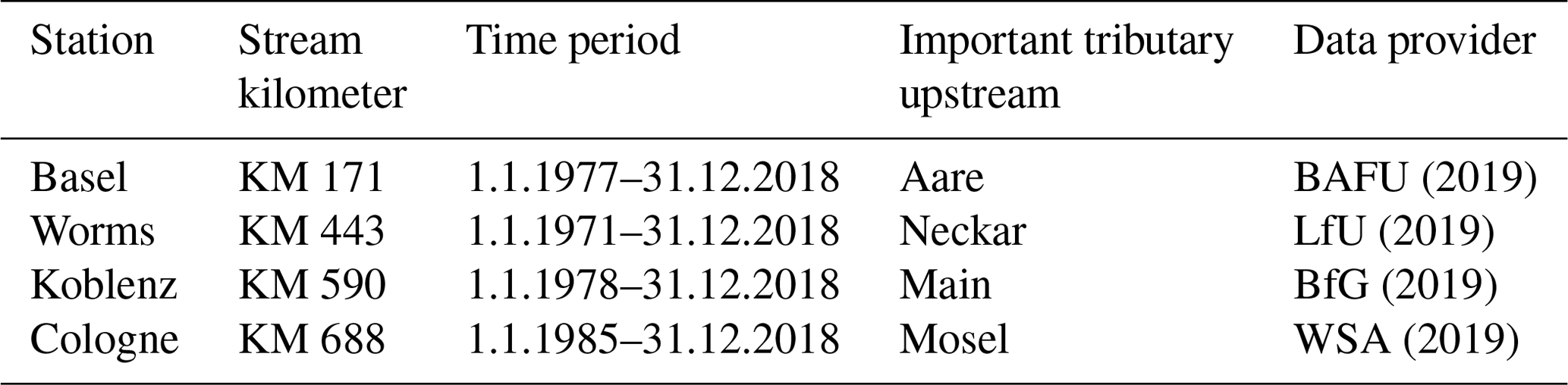
T_w was measured by platinum resistivity sensors (Pt100). The accuracy of these sensors is commonly ±0.5 ^∘C, but the precision, which describes the ability to detect temperature changes, is 0.05 ^∘C. As we focused on the change of T_w over time and did not compare the absolute temperature, the accuracy was not essential, and the precision of the sensors was sufficient for this study. Measurement uncertainties (e.g., depth and location of the sensor) did not influence the calculation with respect to the aim of this study, as long as the measured T_w was a linearly dependent proxy for the average river temperature. Q was provided as daily averages in m³ s⁻¹ by the source in Table 1 and usually calculated from a river stage nearby.

The original data sets were provided by the state and federally operated monitoring stations, which usually run backup measurement systems. They verified the data, and we additionally screened the data set for suspicious features. Missing data points for up to 1 week were linearly interpolated. Longer or recurring data outages were not given.

2.2 Air temperature

T_a is retrieved from the European Centre for Medium-Range Weather Forecasts (ECMWF) Reanalysis Model ERA5. It provides an hourly time resolution of the 2 m T_a on a $\frac{\mathrm{1}}{\mathrm{4}}$^∘ by ${\frac{\mathrm{1}}{\mathrm{4}}}^o$ grid. The data set is available from 1979 to 2018. We took the hourly T_a output and calculated a daily mean for each grid point between 1979 and 2018 to fit the time resolution of T_w.

2.3 Nuclear power plants

The annual electrical power production (EPP) by NPPs is available from the International Atomic Energy Agency (IAEA) Power Reactor Information System (PRIS; IAEA, 2019). A total of 12 NPPs (1986–1988) were online in the Rhine catchment area, and eight remained operational by July 2019. All shutdowns were undertaken in Germany. In this study, separate reactor blocks of the same plant NPPs were combined.

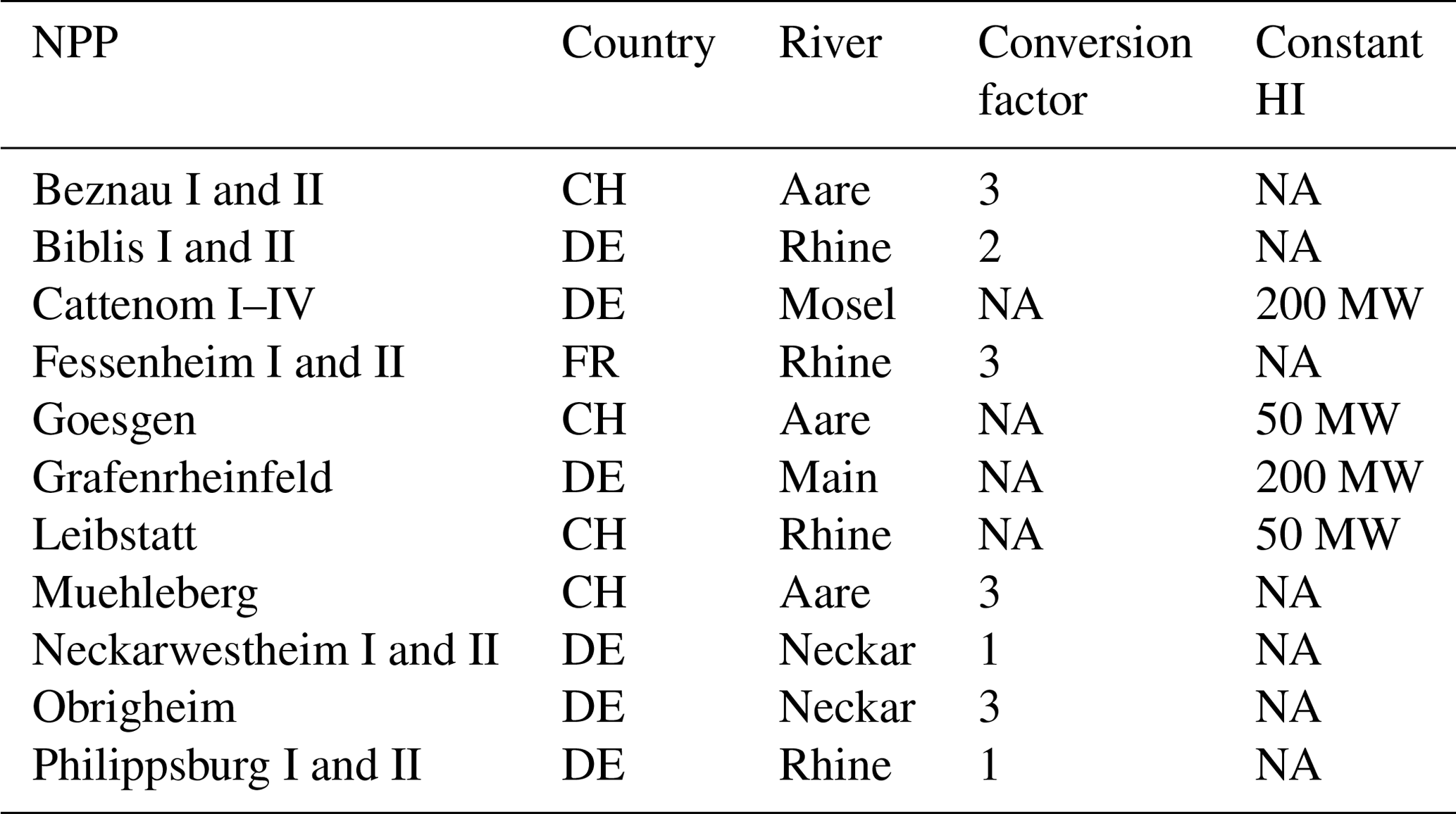
The heat input (HI) by NPPs to the Rhine was calculated for each monitoring station using the conversion factor c and the yearly EPP; see Eq. (2). NPPs with an exclusive river water cooling system have a conversion factor of 3, which is based on the power efficiency of electricity generation (Lange, 2009). Other factors are estimated depending on the cooling system and personal communication with technicians from NPPs. If no conversion factor was available, a constant HI was assumed (Lange, 2009).

$$\begin{array}{}\text{(2)}& \mathrm{HI}\left[\mathrm{GW}\right]={\displaystyle \frac{c\cdot \mathrm{EPP}\left[\mathrm{GWh}\right]}{\mathrm{365}\cdot \mathrm{24}\left[\mathrm{h}\right]}}.\end{array}$$

The NPPs, their conversion factor and, if applicable, the constant HI are shown in Table 2. The time series of upstream HI by NPPs for each monitoring station is shown in Fig. 1.

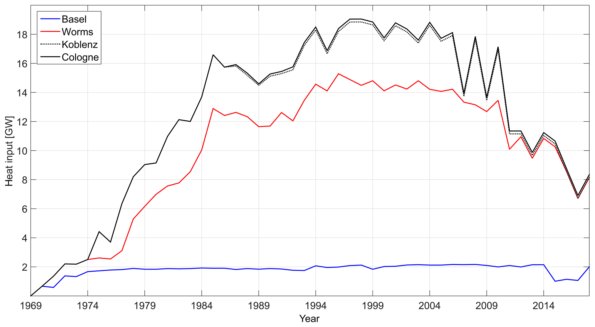
Figure 1 Heat input by upstream nuclear power plants (NPPs) from 1969 to 2018 at each monitoring station.

Table 2 NPPs included in this study. The conversion factor describes the conversion from electrical power production (EPP) to heat input (HI). If cooling towers are installed, a constant heat input was used for the calculation based on Lange (2009). Note: NA – not available.

Calculated temperature change

We calculated the expected change ΔT_w based on a change in HI (Δ HI) from NPPs using the average discharge $\stackrel{\mathrm{‾}}{Q}$, the heat capacity of the water c_p and the water density ρ; see Eq. (3).

$$\begin{array}{}\text{(3)}& \mathrm{\Delta }{T}_{\mathrm{w}}={\displaystyle \frac{\mathrm{\Delta }\mathrm{HI}}{c_{\mathrm{p}}\cdot \stackrel{\mathrm{‾}}{Q}\cdot \mathit{\rho }}}.\end{array}$$

This approach follows the idea that the contribution of NPPs significantly alters the T_w and only influences the RBT fraction.

2.4 Gross domestic product (GDP)

The GDP for the adjacent German federal states is obtained from Arbeitskreis VGdL (2019a, 2007b). Due to changes in the calculation method of the GDP before and after the German reunification (1990), two separate data sets were used. For this study, only the GDP change in the secondary sector (construction and production) was taken into account.

The RBT, if compared to the GDP, was filtered using a 10th order Butterworth bandpass filter. The sampling rate of the GDP was 1 yr⁻¹. We used 1.1 yr⁻¹ as higher and 0.05 yr⁻¹ as lower cutoff frequencies for RBT. This means that signals with a periodicity larger than 20 years and lower than 0.9 years were excluded from the calculations and display. The reasoning for this was to make the RBT data comparable to the yearly data of the GDP change. The low-frequency cutoff was canceling long-term trends, as the GDP change was only related to the previous year. The high-frequency cutoff was used to dampen fast, alternating RBT signals in comparison to the slow sampled GDP data.

2.5 Rescaled adjusted partial sums

Rescaled adjusted partial sums (RAPSs) were used to visualize trends in time series which may not be clearly visible in the unprocessed data set. Equation (4) shows the calculation of the RAPS index X, using time series Y.

$$\begin{array}{}\text{(4)}& X_k=\sum _{i=\mathrm{1}}^{i=k}{\displaystyle \frac{Y_i-\stackrel{\mathrm{‾}}{Y}}{{\mathit{\sigma }}_Y}}.\end{array}$$

$\stackrel{\mathrm{‾}}{Y}$ is the average over the total time series, σ is the standard deviation of the whole time series and Y_i is the ith data point in Y.

A change in the slope of the RAPS index only indicates a change in the slope of the original time series. A negative RAPS slope does not indicate a negative slope in the original time series. Garbrecht and Fernandez (1994) and Basarin et al. (2016) used this method to investigate trends in hydrological time series.

2.6 Catchment area

The catchment area was calculated using the HydroSHEDS database (Lehner et al., 2008). The $\frac{\mathrm{1}}{\mathrm{125}}$^∘ by $\frac{\mathrm{1}}{\mathrm{125}}$^∘ gridded data set provides the information, at each grid point, according to which cell the water of a grid cell is drained. By selecting a starting location, e.g., Koblenz at 50.350^∘ N and 7.602^∘ E, it was possible to iteratively identify all grid points draining into this location. These grid points represent the catchment area of this location (in the example from Fig. 2 at Koblenz). By counting the iteration steps, the distance a water drop travels to reach the monitoring station of Koblenz was determined. This was done for each of the four stations. Additionally, the accumulation number (ACC) was obtained from the data set. It defines how many cells in total were draining into a particular cell, and it is a measure for the size of a river. Finally, a grid, which defines the catchment area, the ACC and the hydrological distance, was established, spanning the whole catchment area. Figure 2 shows the catchment area, the hydrological distance and the calculated flow time to the Koblenz monitoring station.

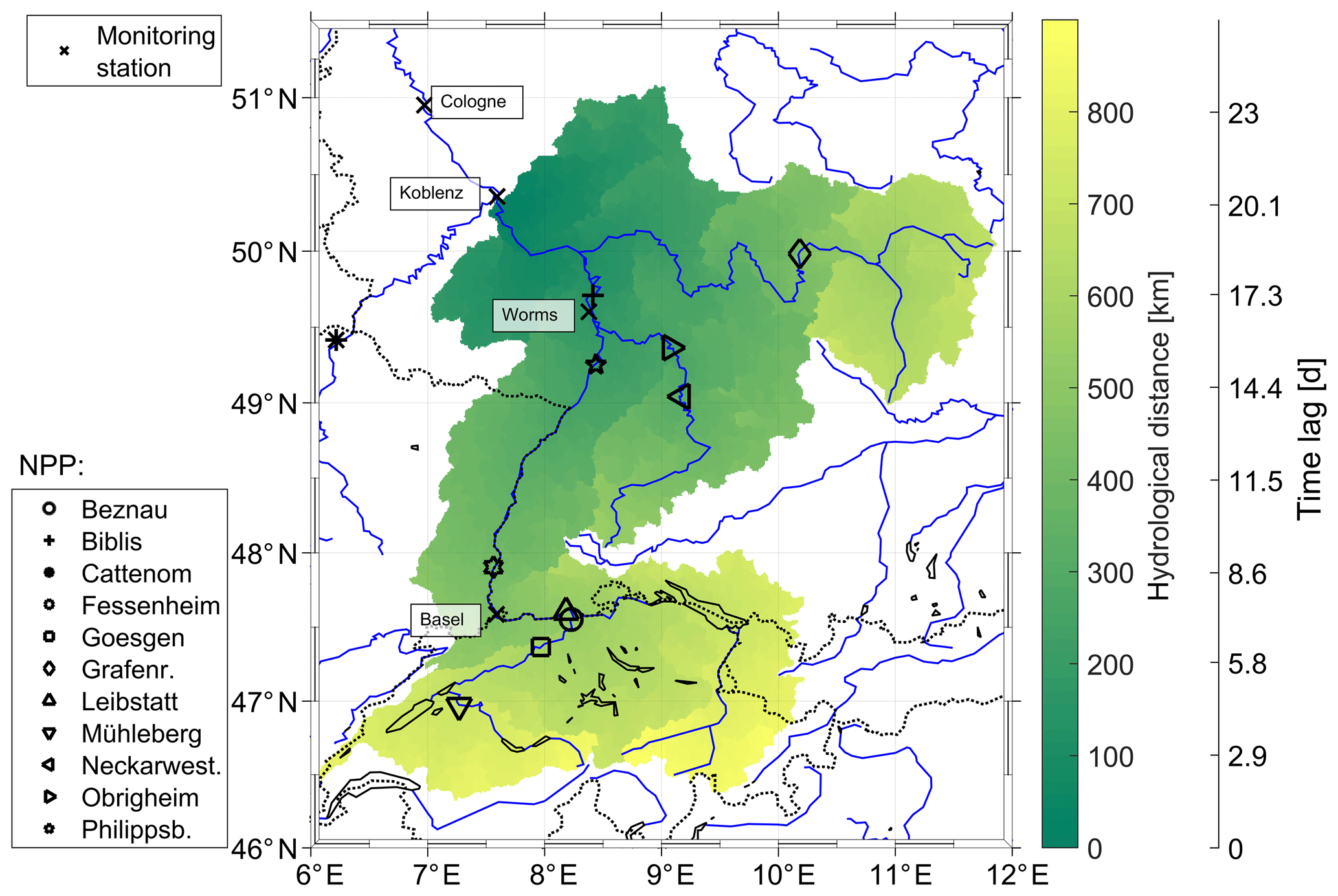
Figure 2 Catchment area of the Koblenz monitoring station as an example. The colors show the hydrological distance between the monitoring station and each grid point of the catchment area. The second y axis shows the time it takes in days, in our setup, to flow from a certain grid point to the monitoring station, based on the hydrological distance. The flow speed is 0.4 m s⁻¹ and was defined to be constant in space and time. All monitoring stations are marked by a cross. The other markers show the location of the NPPs.

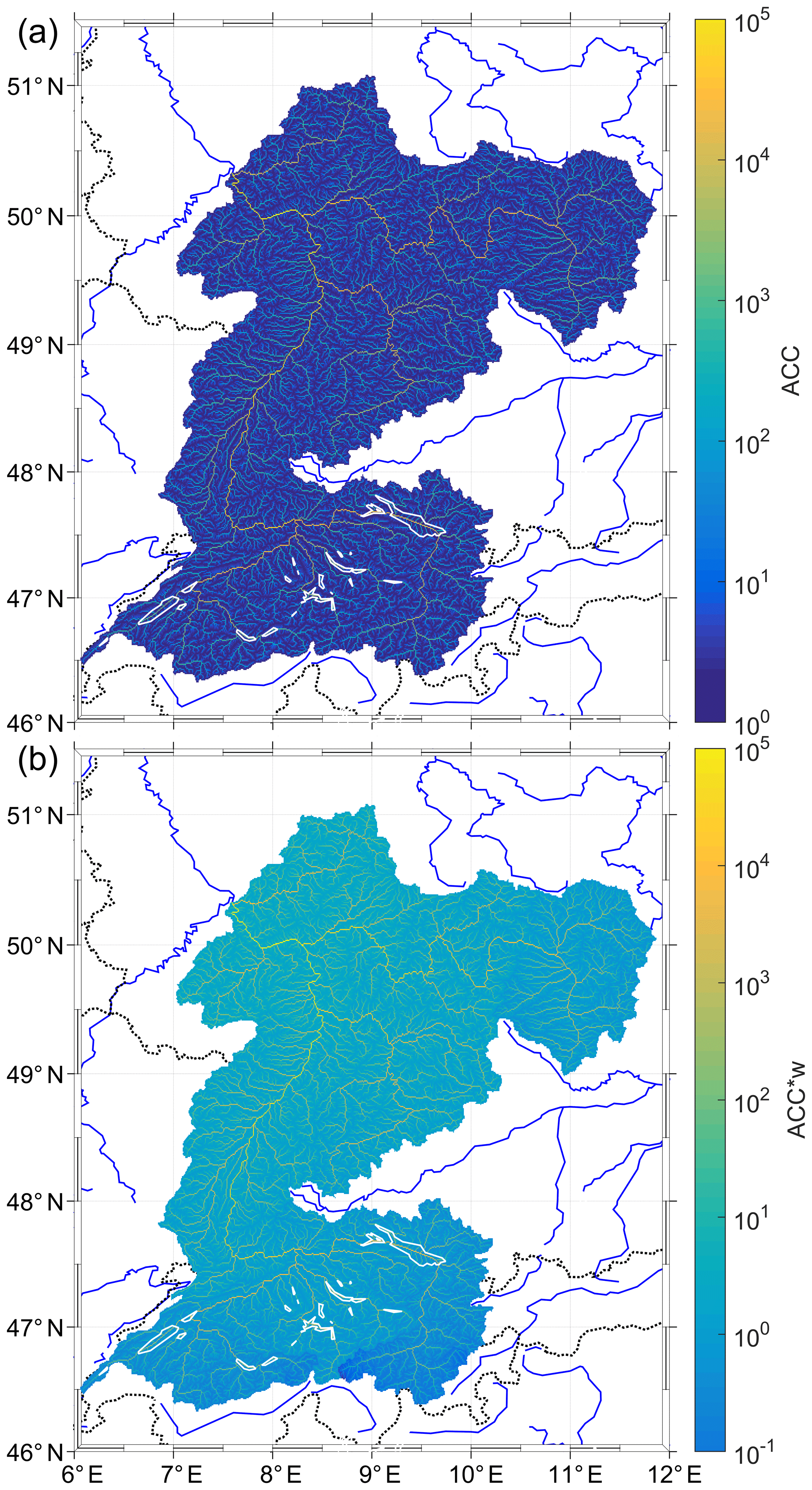
Figure 3 The catchment area of the Koblenz monitoring station. (a) Number of grid points (accumulation number – ACC) which are upstream of each specific grid point. (b) ACC ⋅w, distance and ACC-weighed grid cells.

2.7 Multiple regression

A multiple linear regression was used to separate the anthropogenic heat input a₁ and meteorological a₂ and hydrological a₃ contributions to the river water temperature. T_w was regressed with T_c and river discharge Q. Their regression coefficients a₂ (T_c slope) and a₃ (Q slope) represent the magnitude of the respective influences. The offset a₁ (RBT) combines all other influences which were not related to a change in T_c or Q. We hypothesized that the RBT is directly linked to heat input by power plants, which are NPPs in this study, and other industrial facilities.

Instead of taking T_a directly at the monitoring station, we improved Eq. (1) by a time-dependent and weighed average of T_a ($x,y,t$) over the whole catchment; see Eq. (5). There were spatial coordinates (x,y) in the catchment area, and the subscript ₀ marks the location of the monitoring station.

$$\begin{array}{}\text{(5)}& \begin{array}{rl}{T}_{\mathrm{w}}\left(x_{\mathrm{0}},y_{\mathrm{0}},t_{\mathrm{0}}\right)& =a_{\mathrm{1}}+a_{\mathrm{2}}\cdot T_{\mathrm{c}}\left(x_{\mathrm{0}},y_{\mathrm{0}},t_{\mathrm{0}}+\mathrm{\Delta }t\left(x,y\right)\right)\\ & +a_{\mathrm{3}}\cdot Q\left(x_{\mathrm{0}},y_{\mathrm{0}},t_{\mathrm{0}}\right).\end{array}\end{array}$$

The new representative catchment temperature was called $T_{\mathrm{c}}\left(x_{\mathrm{0}},y_{\mathrm{0}},t_{\mathrm{0}}\right)$. It was a weighed average of the whole catchment area (x,y), which is defined by the measurement point (x₀,y₀). The difference between the measurement time t₀ and the reading of T_a is called time lag Δt(x,y) and depends on the hydrological distance between the measurement point and the reading. Δt(x,y) is negative and points to a moment in time before the measurement.

2.7.1 Time lag

A change in T_w is slower than a change in T_a. The time lag Δt describes this lag and is commonly used in water temperature models.

A reason for the occurrence of Δt is that the water mass mixing capability, heat capacity and surface area cause strong thermal inertia. Changing T_w through new meteorological conditions and heat fluxes takes time. Therefore, linear and exponential models include either a fixed Δt for T_a (Eq. 6) or an average of T_a, including a time span from before (Eq. (7); Stefan and Preudhomme, 1993; Webb and Nobilis, 1995, 1997; Haag and Luce, 2008; Benyaha et al., 2008).

$$\begin{array}{}\text{(6)}& {\displaystyle }{T}_{\mathrm{c}}\left(x_{\mathrm{0}},y_{\mathrm{0}},t_{\mathrm{0}}\right)=T_{\mathrm{a}}\left(x_{\mathrm{0}},y_{\mathrm{0}},t_{\mathrm{0}}+\mathrm{\Delta }t\right)\text{(7)}& {\displaystyle }{T}_{\mathrm{c}}\left(x_{\mathrm{0}},y_{\mathrm{0}},t_{\mathrm{0}}\right)=\sum _{t=t_{\mathrm{0}}}^{t=t_{\mathrm{0}}+\mathrm{\Delta }t}{T}_{\mathrm{a}}\left(x_{\mathrm{0}},y_{\mathrm{0}},t\right).\end{array}$$

A second reason for the mismatch is advection. Rivers, in this case the Rhine, exhibit current velocities which enable their water to cover significant distances on timescales larger than days. Therefore, it is necessary to take the change in T_a, in space and time, during advection into account. This is especially important for daily averaged T_w (Erickson and Stefan, 2000). Pohle et al. (2019) average 8 d of hydroclimatic variables over the whole catchment area; see Eq. (8). However, this approach does not include the characteristics of flow path and flow speed.

$$\begin{array}{}\text{(8)}& T_{\mathrm{c}}\left(x_{\mathrm{0}},y_{\mathrm{0}},t_{\mathrm{0}}\right)=\sum _{x=\mathrm{0},y=\mathrm{0},t=t_{\mathrm{0}}}^{x=n,y=m,t=t_{\mathrm{0}}-\mathrm{8}}{T}_{\mathrm{a}}\left(x,y,t\right).\end{array}$$

We combined the general idea of a time lag and averaging T_a over the whole catchment area (see Eqs. 6, 7 and 8), but in this study, each grid point was linked to a specific time lag Δt(x,y) which is dependent on a fixed flow speed v and the hydrological distance s(x,y) to the measurement point (see Fig. 2). The distance was obtained from the discharge map (Sect. 2.6) and calculated with v, as described by Eq. (9). The new Δt(x,y) represents the mismatch by advection but not specifically the mismatch through thermal inertia. The thermal inertia would be independent of s(x,y) and a constant added to Δt. However, we are of the opinion that a sufficient part of the thermal inertia time lag was included in our representation of Δt(x,y).

$$\begin{array}{}\text{(9)}& \mathrm{\Delta }t\left(x,y\right)=-{\displaystyle \frac{s\left(x,y\right)}{v}}.\end{array}$$

2.7.2 Weighing coefficients

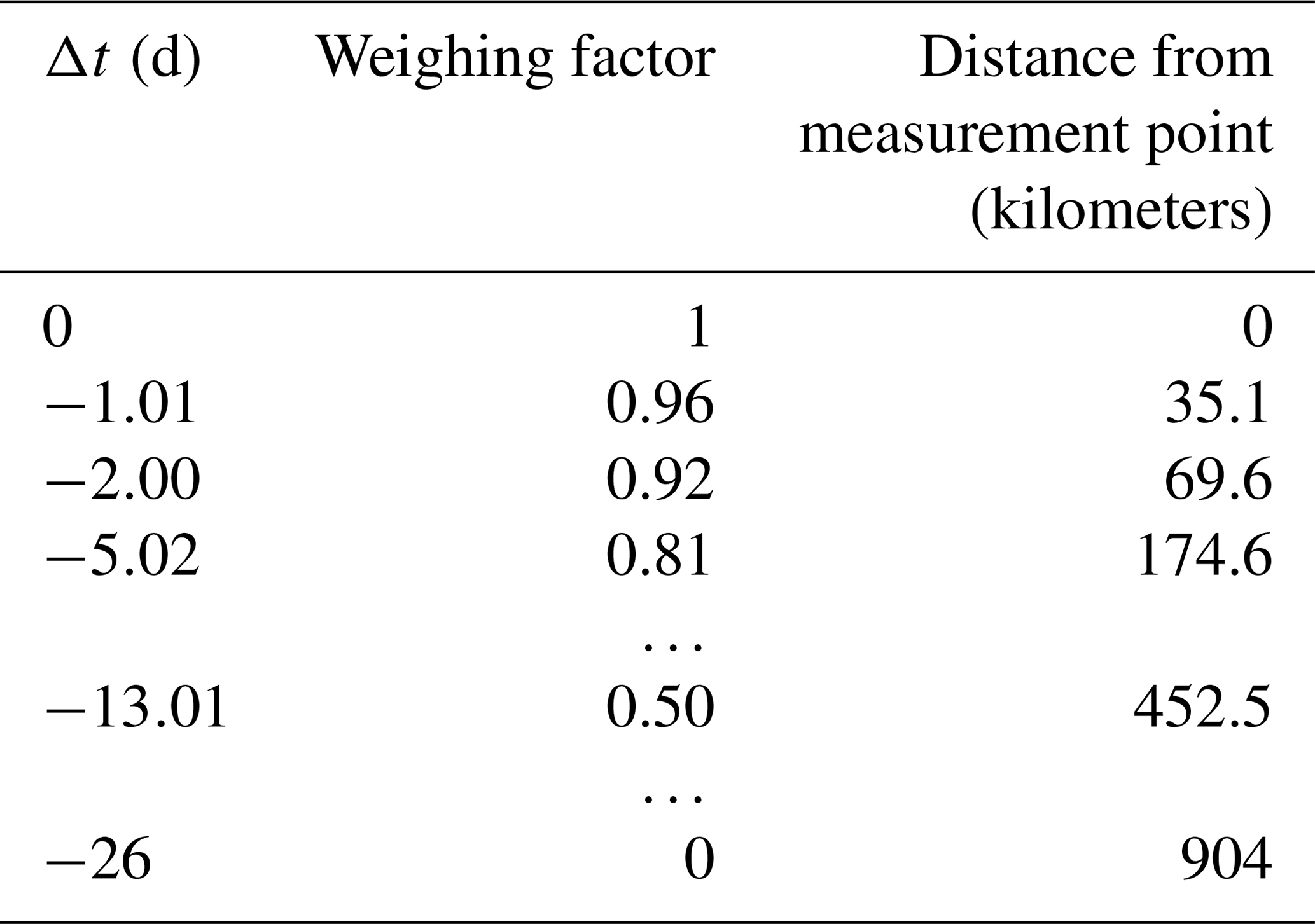
Tobler (1970) proposed that close spatial and temporal conditions tend to be more highly correlated than those further away. This led to the introduction of the weighing factor w. A linear decreasing weighing factor from 1 to 0 was used; 1 marks the grid point closest (smallest Δt) to the monitoring station and 0 the point farthest away (largest Δt). As the sizes of the catchment areas were different for the four monitoring stations, four weighing coefficient tables were calculated. As an example, Table 3 shows the weighing coefficient for Koblenz.

Table 3 Weighing factors for the distance and the resulting Δt for the monitoring station of Koblenz. Δt is calculated from distance and flow speed; see Eq. (9). The weighing coefficient is linearly correlated to Δt.

A catchment-wide hydrological flow model, estimating the flow speed at every grid point for every hydrological scenario, was not used. It was not available yet for every grid point of the catchments, and the focus of this study was to create a simple setup that is also transferable to other river catchments. Therefore, using a constant flow speed of 0.4 m s⁻¹ was decided on. This flow speed was determined by calculating the root mean square error (RMSE; whole data set) of the ACC +Δt model, with a step-wise reduction in the flow speed from 1.4 to 0.3 m s⁻¹. The lowest RMSE was obtained at Koblenz at 0.4 m s⁻¹. The RMSE and Nash–Sutcliffe coefficient (NSC) coefficients at all flow speeds and all stations are shown in the Supplement. For Basel and Worms, slower flow speeds lowered the RMSE further. We did not include this as it would create unreasonable low flow speeds. The reason for the low flow speeds, with lowest RMSE, might be the thermal inertia. As thermal inertia is not explicitly represented in Δt (Eq. 9), a smaller flow speed could compensate for that, especially in smaller catchment areas.

The weighing coefficient w is combined with ACC. ACC is used as a second coefficient which overweighs grid points with large accumulation and, therefore, large water masses. This ensures a balance between the large number of low ACC grid points, which carry less water, and the influence of T_a on large water masses. Figure 3b shows ACC ⋅w over the whole catchment area of Koblenz.

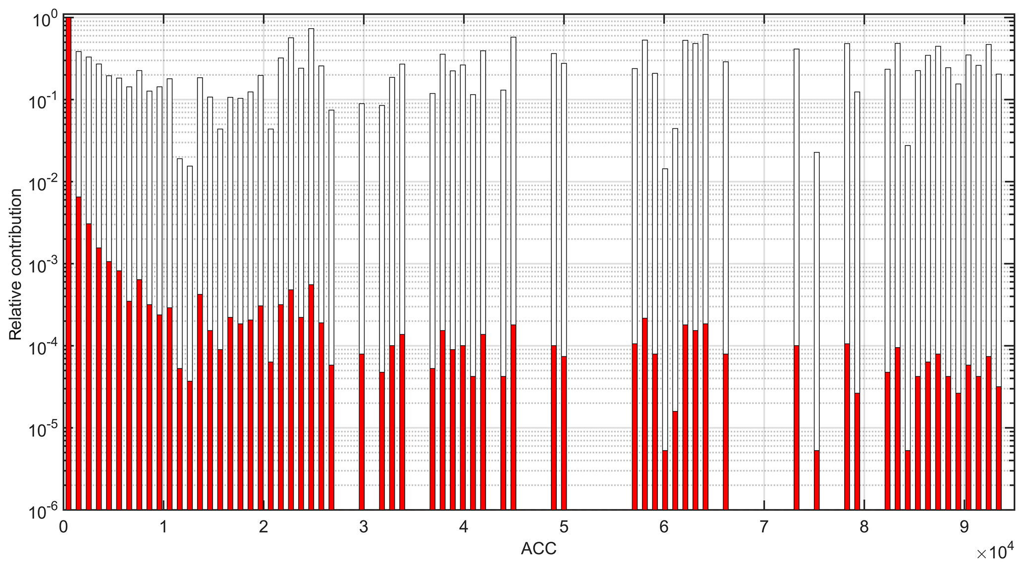
Figure 4 ACC bins (x axis) vs. the relative contribution (y axis). The grid points are binned by their ACC value. The red bars show the relative contribution (largest contribution normalized to one) by the number of grid points in this bin only. The white bars show the distribution using the number of grid points in this bin and weighing ACC ⋅w.

2.7.3  T_c

Combining Δt, ACC ⋅w weighing and the gridded temperature reanalysis data of Sect. 2.2, we proposed a new 3D $\left(x,y,t\right)$ averaging of T_a, which is shown in Eq. (10).

$$\begin{array}{}\text{(10)}& \begin{array}{rl}{T}_{\mathrm{c}}& \left(x_{\mathrm{0}},y_{\mathrm{0}},t_{\mathrm{0}}\right)={\displaystyle \frac{\mathrm{1}}{n\cdot m}}{\displaystyle \frac{\mathrm{1}}{\sum w\left(\mathrm{\Delta }t\left(x,y\right)\right)\cdot \mathrm{ACC}\left(x,y\right)}}\\ & \sum _{x=\mathrm{1},y=\mathrm{1}}^{x=n,y=m}w\left(\mathrm{\Delta }t\left(x,y\right)\right)\cdot \mathrm{ACC}\left(x,y\right)\\ & \cdot T_{\mathrm{a}}\left(x,y,t_{\mathrm{0}}+\mathrm{\Delta }t\left(x,y\right)\right).\end{array}\end{array}$$

$T_{\mathrm{c}}\left(x_{\mathrm{0}},y_{\mathrm{0}},t_{\mathrm{0}}\right)$ was calculated by weighed (ACC ⋅w) averaging $T_{\mathrm{a}}\left(x,y,t+\mathrm{\Delta }t\left(x,y\right)\right)$ over all grid points of the catchment area ($x=\mathrm{1},\mathrm{\dots }ny=\mathrm{1},\mathrm{\dots }m$), which was set by the measurement point (x₀,y₀). The time lag Δt was an estimate for the time it takes a water droplet from a specific grid point (x,y) in the catchment area to reach the measurement location.

Based on Eq. (10), the daily T_c was calculated for each monitoring station. This temperature represents the meteorological influence all water droplets have experienced on their way to the monitoring station and is subsequently used in the multiple linear regression.

2.7.4 T_c calculation methods

Additionally, we used these four calculations methods, namely (1) w+Δt, (2) avg +Δt, (3) avg and (4) point, to compare the results of the linear regression to the calculation proposed in Eq. (10).

(1) In the following, only w weight (Eq. 11) and time lag are shown:

$$\begin{array}{}\text{(11)}& \begin{array}{rl}{T}_{\mathrm{c}}& \left(x_{\mathrm{0}},y_{\mathrm{0}},t_{\mathrm{0}}\right)={\displaystyle \frac{\mathrm{1}}{n\cdot m}}{\displaystyle \frac{\mathrm{1}}{\sum w\left(\mathrm{\Delta }t\left(x,y\right)\right)}}\\ & \sum _{x=\mathrm{1},y=\mathrm{1}}^{x=n,y=m}w\left(\mathrm{\Delta }t\left(x,y\right)\right)\cdot T_{\mathrm{a}}\left(x,y,t_{\mathrm{0}}+\mathrm{\Delta }t\left(x,y\right)\right).\end{array}\end{array}$$

(2) Here, no weight and only time lag (Eq. 12) are shown, as follows:

$$\begin{array}{}\text{(12)}& T_{\mathrm{c}}\left(x_{\mathrm{0}},y_{\mathrm{0}},t_{\mathrm{0}}\right)={\displaystyle \frac{\mathrm{1}}{n\cdot m}}\sum _{x=\mathrm{1},y=\mathrm{1}}^{x=n,y=m}{T}_{\mathrm{a}}\left(x,y,t_{\mathrm{0}}+\mathrm{\Delta }t\left(x,y\right)\right).\end{array}$$

(3) A mean $T_{\mathrm{a}}(x_{\mathrm{0}},y_{\mathrm{0}},t_{\mathrm{0}})$ over the whole catchment area at the time t₀ of the measurement was calculated; see Eq. (13). Δt was not used in the following:

$$\begin{array}{}\text{(13)}& \begin{array}{rl}w\left(x,y\right)& =\mathrm{1}\\ & T_{\mathrm{c}}\left(x_{\mathrm{0}},y_{\mathrm{0}},t_{\mathrm{0}}\right)={\displaystyle \frac{\mathrm{1}}{n\cdot m}}\sum _{x=\mathrm{1},y=\mathrm{1}}^{x=n,y=m}{T}_{\mathrm{a}}\left(x,y,t_{\mathrm{0}}\right).\end{array}\end{array}$$

(4) $T_{\mathrm{a}}(x_{\mathrm{0}},y_{\mathrm{0}},t_{\mathrm{0}})$ at the location x₀,y₀ and time t₀ of the measurement (see Eq. 14) is shown, as follows:

$$\begin{array}{}\text{(14)}& T_{\mathrm{c}}\left(x_{\mathrm{0}},y_{\mathrm{0}},t_{\mathrm{0}}\right)=T_{\mathrm{a}}\left(x_{\mathrm{0}},y_{\mathrm{0}},t_{\mathrm{0}}\right).\end{array}$$

3 Results

3.1 Water temperature time series

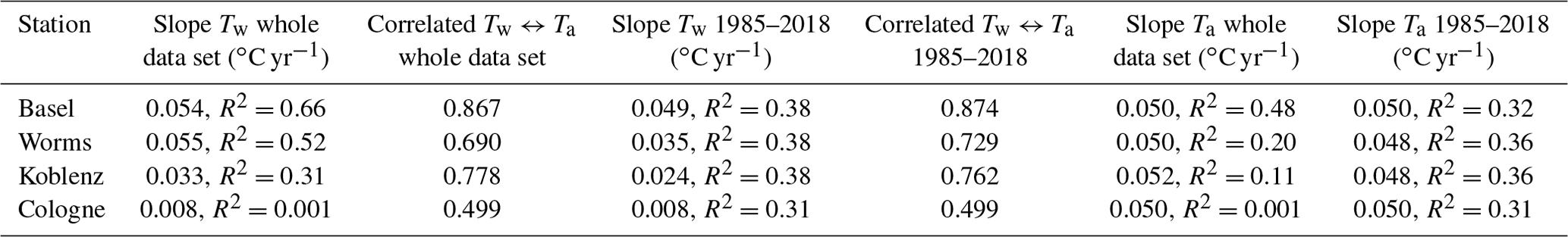
To investigate the long-term changes, we fitted a time-dependent linear function to the time series of T_w and T_a (catchment average) of all four monitoring stations (Basel, Worms, Koblenz and Cologne). The same was also done when all four monitoring stations had an overlapping data set (1985–2018); see Table 1. Figure 5a presents the yearly averaged T_w and the linear fits for the two time periods. The average T_a of the catchment area is also shown. In Fig. 5b, the RAPS index of T_a and T_w is shown. The fit coefficients and the rate of warming per year are displayed in Table 4. The calculated T_a increased in the catchment area of all monitoring stations, and the respective slopes are shown in columns four and five of Table 4.

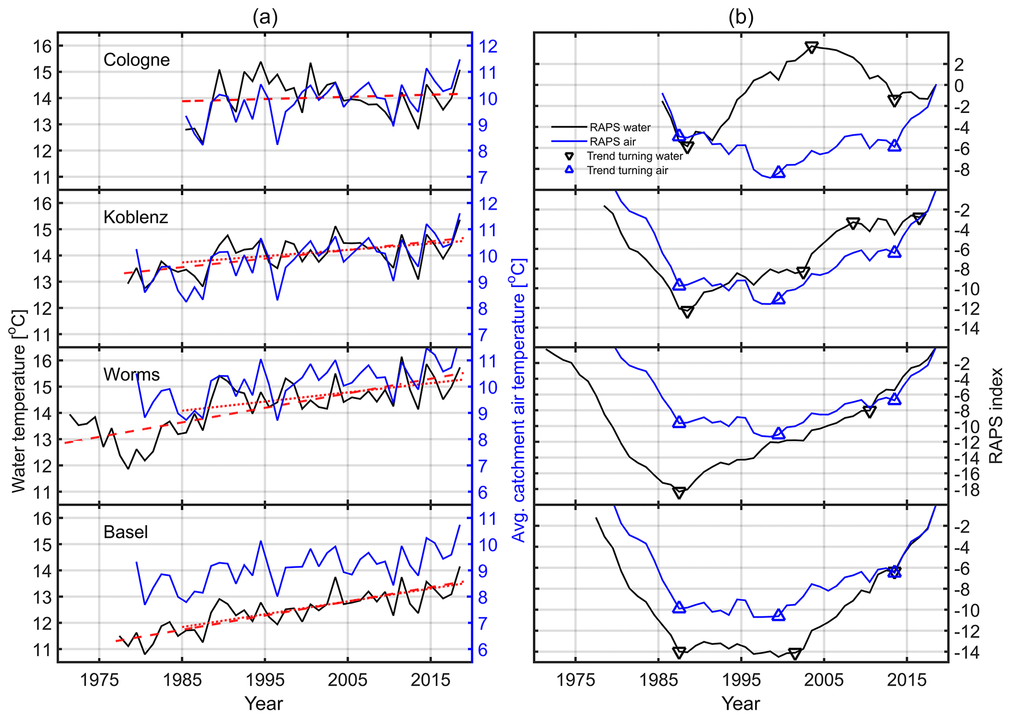
Figure 5 (a) Yearly averages of water temperatures at the four monitoring stations (black line). The red dashed line is a fit to the available data set. The red dotted line is a fit to the overlapping time period (1985–2018). The blue line is the yearly average air temperature of the catchment area. (b) RAPS T_w (black) and T_a (blue) indexes. The triangle markers divide the RAPS index into sections, based on a slope change in the RAPS index. Each section also represent a trend change in the original T_a and T_w time series.

Figure 5 and Table 4 show that the change in T_w was found to be heterogeneous along the Rhine. The slope at Basel is approx. 6 times higher (0.049 ^∘C yr⁻¹) than the one at Cologne (0.0084 ^∘C yr⁻¹), when comparing only the overlapping data set. However, during the same period, T_a (0.05 ^∘C yr⁻¹ at Basel; 0.05 ^∘C yr⁻¹ at Cologne) displays similar behavior at these two stations, which is an indication of a similar meteorological influence. The T_w warming rate from 1985 to 2018 for Worms and Koblenz is in between those from Cologne and Basel. These two stations show similar T_a warming rates compared to Basel and Cologne. Generally, the T_a warming rates have a difference of less than 5 %. Arora et al. (2016) showed a mean T_w warming rate in northern and northeastern German rivers of 0.03 ^∘C yr⁻¹ (1985–2000) and 0.09 ^∘C yr⁻¹ (2000–2010). Regarding our time period (1985–2010), these values are plausible. Basarin et al. (2016) found a maximum increase in T_w at the Danube at Bogojevo (1950–2012) of 0.05 ^∘C yr⁻¹, which matches the maximum increase at Basel. T_a increased by 0.02 ^∘C yr⁻¹ between 1985 and 2010 in the study by Arora et al. (2016). We found a steeper slope at all stations. The reason could be the hiatus of global warming (Hartmann et al., 2014), which is a flattening of the T_a increase between 1998 and 2012. This period is fully included in the Arora et al. (2016) study and our data set, but we investigated further until 2018, when the warming of T_a already increased again (Hu and Fedorov, 2017). Michel et al. (2020) investigated T_w at 52 river gauges in Switzerland, representing most of the Rhine catchment area at Basel. The authors reported an average T_w increase at the 52 stations of 0.037 ^∘C yr⁻¹ (1998–2018) and 0.033 ^∘C yr⁻¹ (1979–2018). T_a increased by 0.039 ^∘C yr⁻¹ (1998–2018) and 0.046 ^∘C yr⁻¹ (1979–2018). Comparing this to our results at Basel, the T_a warming rates are similar. The difference might originate from the use of meteorological stations nearby river gauges only (Michel et al., 2020) instead of a reanalysis product. The difference in T_w warming (approx. 0.021 ^∘C yr⁻¹) could be interpreted as showing that most warming might occur in the broader vicinity before the Basel monitoring station.

The R² values make the differences between the four monitoring stations visible. Basel exhibits the largest R² values, and these are consistently high for T_a and T_w. This is in contrast to the station at Cologne, where R² of T_w was low and statistically not significant. The slope of T_a at Cologne is lower than at the other stations but still statistically significant. The Pearson correlation coefficients between T_a and T_w were the lowest at Cologne and the largest in Basel. For T_a, the RAPS index of all the monitoring stations showed four concurrent sections (start–1987, 1987–2000, 2000–2014 and 2014–end). Their borders are marked by the blue triangles in Fig. 5. The section between 2000 and 2014 could be a consequence of the hiatus of global warming between 1998 and 2012 (Hartmann et al., 2014). Each section represents slope changes in the RAPS index and indicates trend changes in the original time series. The T_w RAPS index for Basel displayed the same pattern in the sections as the T_a index. All other stations showed other RAPS T_w to RAPS T_a patterns. This means that the T_a and T_w trends of the original time series were different at these stations. T_a cannot fully describe the trends in T_w.

We hypothesized that different meteorological conditions were not the reason for this difference. Meteorological differences should also have been visible in the T_a warming rate of the four stations, which was not the case. The RAPS analysis for T_a and T_w only coincided within the Basel data set.

Table 4 Slope of linear fits and Pearson correlation coefficients to the daily temperature data at the four monitoring stations. The data set used is described in the column header. Next to the slope values are the R² values, which are statistically significant if R²>0.19.

3.2 Regression

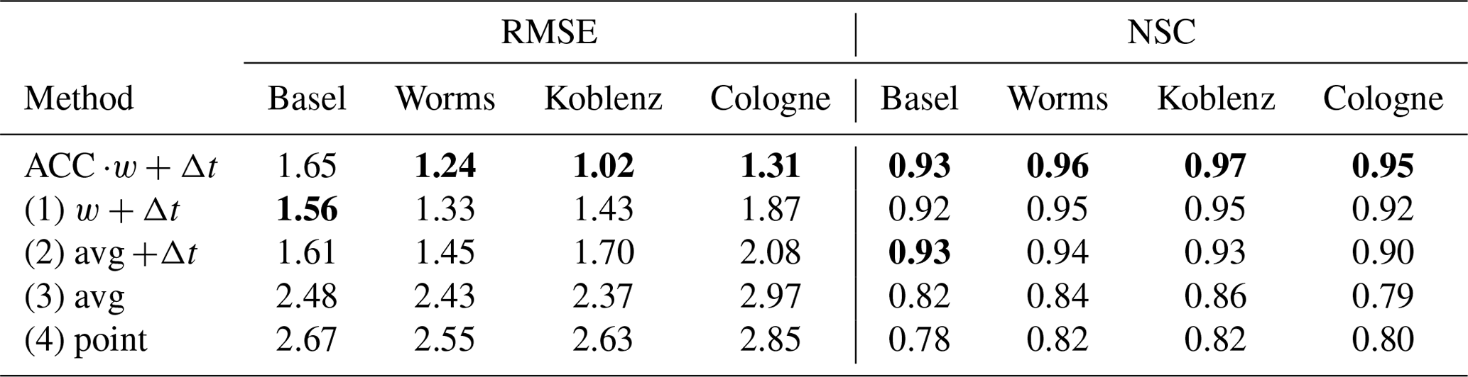
We fitted the multiple regression model (Eq. 5) using T_c and Q to T_w of each monitoring station for the available data set. Afterwards, we recalculated T_w,modelled using the regression coefficients a₁, a₂ and a₃. From the comparison between the T_w,modelled and measured T_w, the RMSE and the NSC for each monitoring station was derived (see Table 5). To support the introduction of weighing coefficients ACC ⋅w and Δt, we compared five different calculations of T_c from Sect. 2.

Table 5 shows the RMSE and NSC values for all correlations. The lowest (RMSE) and highest (NSC) values are displayed in bold in Table 5. The lowest RMSE was found to be 1.02 ^∘C for ACC $\cdot w+\mathrm{\Delta }t$ (first row) at the Koblenz station. At this location, the largest NSC, of 0.97, also appeared. The flow speed was optimized for lowest RMSE at the Koblenz station (see Sect. 2.7.2). It was evident that the three methods, including a Δt, have a lower RMSE (below 2.01 ^∘C; lowest 1.02 ^∘C) than the two methods without a Δt (above 2.37 ^∘C; largest 2.97 ^∘C). The same trend held true for NSC where the Δt methods were above 0.90 and the other two were below 0.86. We think that the use of a catchment-wide Δt improved the quality of the multiple regression analysis and delivered a significant improvement in the T_a→T_w-based modeling. Interestingly, combining ACC and the weighing factor w provided the best estimation for all stations, except for Basel. The content of Fig. 4 could explain this result. Without ACC weighing, small water masses (small ACC) may be overrepresented in the contribution to T_c. Large ACC grid points represent large water masses (rivers and lakes), and their influence on T_a may be otherwise underestimated. At Basel the fraction of lowACC grid points was relatively small compared to the other stations, as Basel is closest to the water sources and has the smallest catchment area. Therefore, the ACC weighing might have provided weaker results.

As ACC $\cdot w+\mathrm{\Delta }t$ provided the smallest RMSE, this calculation method was used for all further calculations of T_c.

In the Supplement, we provide a calculation of the regression coefficients for the year 2001 only. These coefficients were then taken as a basis for calculating T_w for each year from 2000 to 2018. The RMSE and NSC data were consistent in magnitude with the long-term regressions of this section. The RMSE at Koblenz ranged from 0.75 to 1.22 ^∘C. A lower RMSE was caused by the shorter regression period. This supports the stability and validity of the regression model.

Table 5 RSME (in degrees Celsius) and NSC for all T_c calculation methods. Different T_c calculation methods and the regressions are applied over the total data set. The RMSE and the NSC are calculated between T_w and T_w,modelled. The first column contains the calculation method. The best results for each monitoring station and each calculation method are indicated in bold.

3.3 Rhine base temperature

The RBT was used to explain differences in the T_w warming rates of Table 4. We regressed a 2-year segment of the T_w time series and set a step size of 1 month in order to create a RBT time series over the full data set. The regression of a 2-year segment should also compensate for extreme events occurring during 1 year. These could be extremely low discharge or extreme water temperatures in which industrial and power production had to react. As the absolute RBT cannot be meaningfully interpreted, only the changes in RBT over time are shown in Fig. 6. We subtracted the last data point of each time series from the rest of the data and showed the change in RBT, a 4-year running mean and Δ RBT (Eq. 3) vs. time. The HI by NPPs is shown as a dotted blue line relating to the y axis on the right (Fig. 6).

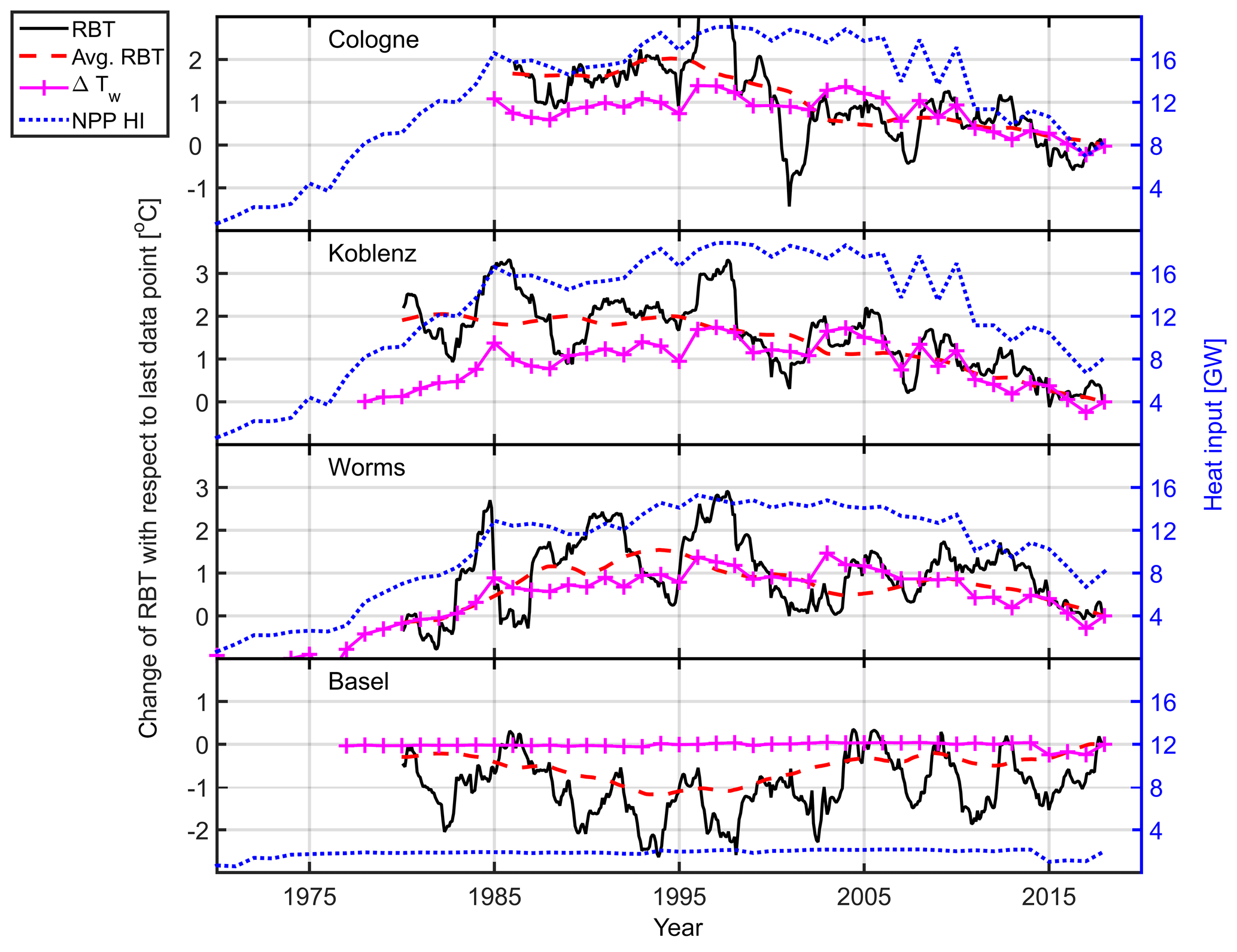
Figure 6 Rhine base temperature (RBT) from four monitoring stations (black solid line). The red dashed line is the RBT 4-year running mean. The magenta line with the “+” markers shows the ΔRBT relative to the last year. The blue dotted line is the upstream heat input (HI) by NPPs; see Sect. 2.3.

3.3.1 Long-term trends

In this study, long-term trends were visible on timescales of decades. The HI by NPPs, the 4-year running mean RBT and ΔRBT followed a similar trend in this analysis (see Fig. 6). After the maximum heat discharge from NPPs between 1996 and 1998, the HI and the RBT of Worms, Koblenz and Cologne declined. The RBT started its decline 1–2 years before 1995, which might have been triggered by the recession in 1993 and a sharp drop in the German trade balance. At Basel, the RBT and the HI remained comparably constant. Additionally, we calculated ΔT_w based on the change in HI, using Eq. (3), at every station and compared it to the ΔRBT from the regression model (see Table 6). The period for each monitoring station starts at the maximum HI by NPPs for the respective station and ends in the year 2017.

Table 6 Change in RBT (column three) in the time period given in column two. The start of the period indicates the maximum HI of NPPs at the respective monitoring station. The calculated ΔT_w (column four) and the change in HI by nuclear power plants (column five) are also provided. The calculations were done using Eq. (3). Note: GW – gigawatt.

At Basel, both simulated and calculated RBT changes were negligible due to the lack of change in HI. At all other stations, the change in HI was reflected in the change in RBT. The maximum difference between simulation and calculation was found to be 0.34 ^∘C. Before 1995, Worms, Koblenz and Cologne showed an approximately 1 ^∘C offset between ΔRBT and ΔT_w (see Fig. 6). This occurred during a time when the NPPs HI remained relatively stable, but the GDP increased by 30 % between 1985 and 1995 (Worldbank, 2020). The change in nuclear power production over a time period of 30 years or more can explain the changes in and the heterogenous warming rates of T_w along the Rhine. NPPs may also impact T_w at much shorter timescales but do not change their power output accordingly.

3.3.2 Short-term trend

Short-term changes (<5 years) in RBT (Fig. 6) are not likely to be influenced by the overall HI from NPPs, as these adopt production at longer timescales. More important are local industrial conditions, which could also include fossil fuel power plants. However, not all influences on the coefficient a₁ and, subsequently, on the RBT originate from industrial production. Various potential influences are unknown and not within the scope of this publication.

For Basel, it was not possible to satisfyingly explain the short-term variations. The Rhine and its tributaries upstream are flowing through subalpine lakes and, in relation to the downstream part, are not strongly industrialized. Lakes have a complicated heat budget (Råman Vinnå et al., 2018), which was not focused on in this analysis.

For all other stations, we hypothesized that local production facilities and their HI into the Rhine are responsible for the short-term changes, by comparing the RBT time series to economic data. Figure 7 shows the comparison of RBT (black line; 1 year running mean) to the changes in the GDP (blue line). A discontinuity in the GDP in 1991 is visible due to the German reunification, which is when the calculation method of the GDP changed. Therefore, the data were plotted as separate lines.

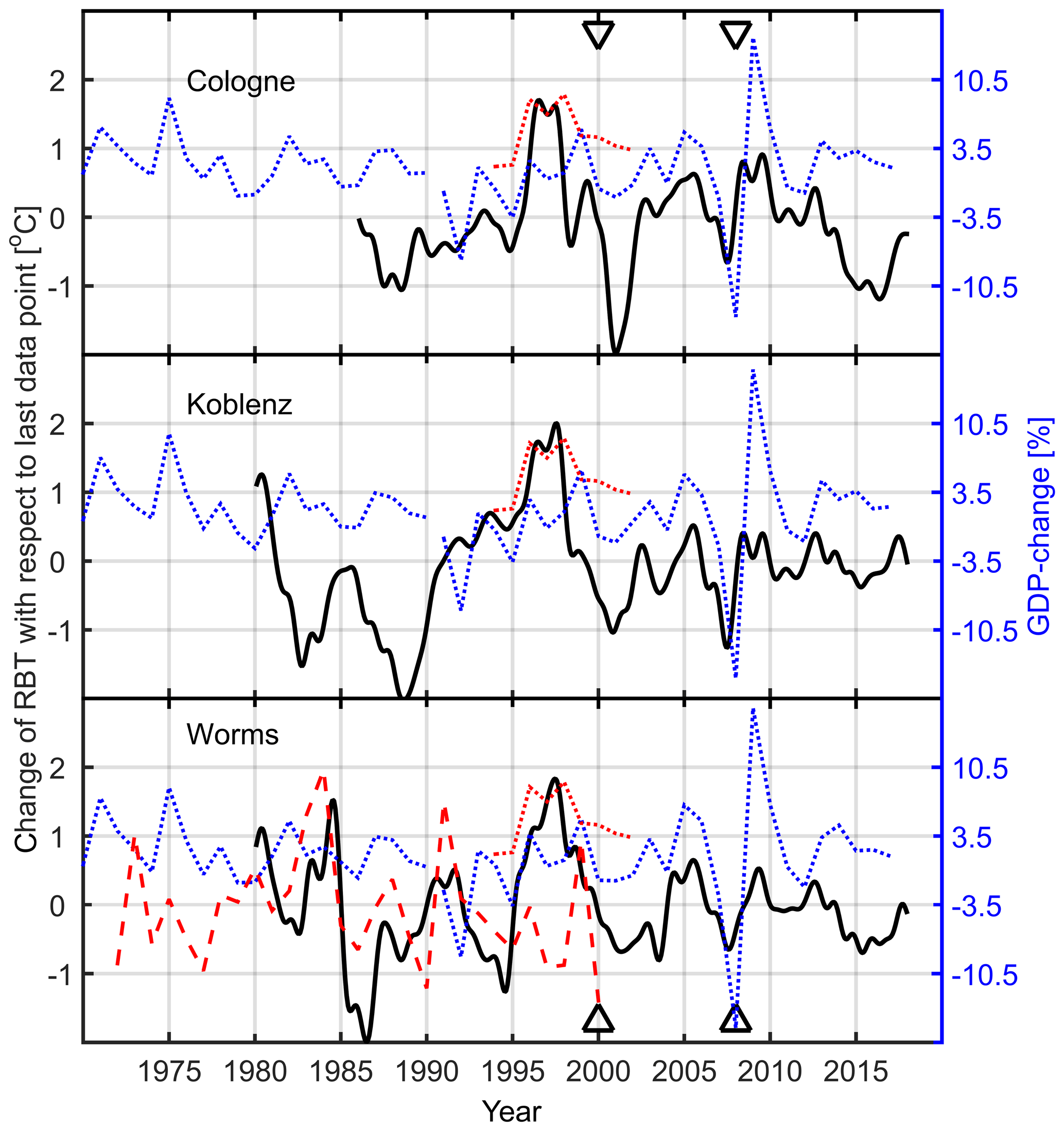
Figure 7 The change in RBT (black solid line) at three monitoring stations (Cologne, Koblenz and Worms). The blue dashed line is the GDP change in the adjacent federal states. To explain trends during two time periods, the red dashed line, which is the turnover of BASF, and the red dotted line, which is the production rate of the oil refineries, were added. The triangles mark the years 2000 (burst of the dot-com bubble) and 2008 (mortgage crisis).

For Worms (Fig. 7, bottom panel), we added the change in the turnover of BASF (red dashed line; BASF AG, 1989). BASF is a major chemical company, and one of its largest production facilities, with an estimated HI of 500 MW to 1 GW, is located 12 km upstream (Rhine kilometer 431) from the Worms station. It was investigated whether the production and HI changes in this factory were also visible. In 1985, although the change in GDP did not indicate a large RBT change, a RBT decrease was visible. This was indicated by a turnover decrease in 1985 and 1986. After the German reunification in 1990, a negative GDP change (recession) was evident. This was followed by a BASF turnover decline and a decrease in RBT. After that, the RBT followed the zigzag movements of the GDP, and so did the BASF turnover (only shown until 2000). In particular, the economic events, such as the burst of the dot-com bubble (early 2000s) and the mortgage crisis (2008), were visible in the RBT and in the GDP when a decrease in both parameters followed. The two events are marked by triangles in Fig. 7.

Before 1990, the RBT at Koblenz did not follow the GDP trend, and it showed a rather anticyclic behavior which can not be explained yet. After 1991, the RBT followed the general trend of the GDP but did not seem to be strongly influenced by the short recession after the German reunification. Again, economic events such as the burst of the dot-com bubble (early 2000s) and the mortgage crisis (2008) displayed an influence on the RBT.

The RBT at Cologne did not seem to be strongly influenced by the recession connected to the German reunification, but after 1999, the RBT follows the zigzag trends of the GDP.

For all monitoring stations, a red dashed line was added between 1995 and 1999. This dashed line indicates the production rate of German oil refineries (MWV, 2003). From 1995 to 1999, German refineries ran at full capacity (100 %); usually the capacity levels did not exceed 90 %. The increase in production was clearly visible in the RBT at Cologne, where a large oil refinery is located 19 km upstream at Rhine kilometer 671 (Rhineland refinery). The RBT at Worms and Koblenz could be influenced by the output of a refinery next to Karlsruhe at Rhine kilometer 367 (Mineraloelraffinerie Oberrhein).

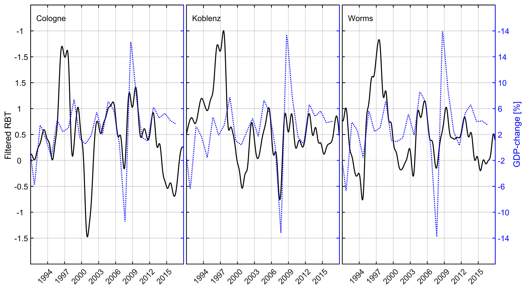
Figure 8 Detrended and filtered RBT signal (black solid) and the GDP change (blue dashed) at Cologne, Koblenz and Worms.

3.3.3 Correlation

We correlated the GDP change and the filtered RBT signal. It was noticeable that a 480 d shift to the past was needed to obtain matching trends. This means that a change in RBT or anthropogenic HI appeared about 480 d earlier than in the GDP calculation. The shift could be caused by the following two reasons: (1) using the GDP difference of 2 consecutive years has a significance at a unspecific point of time within these 2 years. (2) The GDP is lagging behind the real economic situation which is, in this case, the industrial production. Yamarone (2012) claimed that GDP was a coincident economic indicator similar to industrial production. However, Yamarone (2012) used quarterly GDP calculations, and in this study annual data were used. The quarterly data set may react faster to changes. A second thought was that Yamarone (2012) compared the calculations of industrial production, which is an economic index, to GDP (another economic index). In this study, real-time data from industrial HI into the river was processed. This shift has not been done for Fig. 6) because a shift of 1.5 years on a 40-year timescale is negligible.

Table 7 Spearman's rank correlation coefficients between RBT and GDP change for ACC $\cdot w+\mathrm{\Delta }t$. The last column shows the significance.

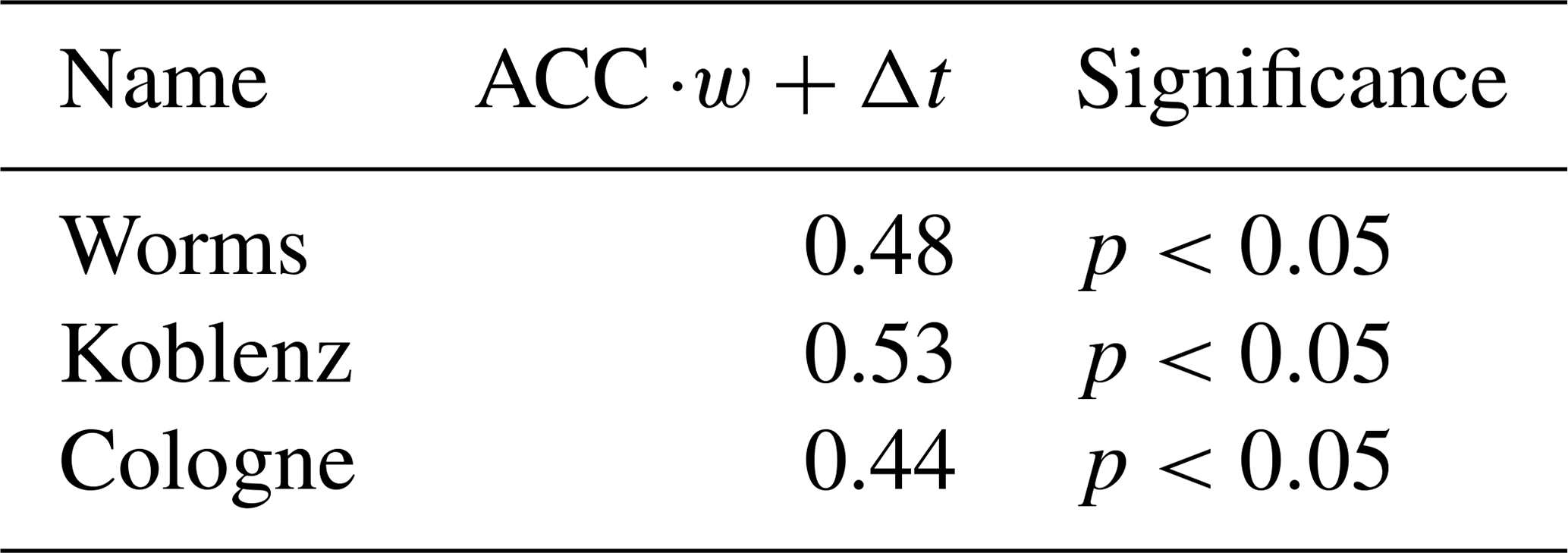
Table 7 shows the Spearman's rank correlation coefficients of Worms, Koblenz and Cologne for the ACC $\cdot w+\mathrm{\Delta }t$ calculation method, which resulted in the lowest RMSE at Koblenz.

All correlations were found to be positive and statistically significant (p<0.05). The correlation at Koblenz was highest. Figure 8 shows the filtered RBT signal vs. the GDP change at the three monitoring stations. The RBT time series was detrended and filtered. Most of the time, the variations in the RBT (filtered and shifted) were coincident with the GDP change. The RBT peak between 1995 and 1998 was not very well represented by the GDP change, which has already been discussed earlier in context of Fig. 7.

4 Conclusions

We introduced a new catchment-wide air temperature T_c, which decreased the RMSE (Table 5) in a T_c→T_w regression. T_c is a weighed (ACC ⋅w) average of all T_a across the catchment area, including the use of Δt for each grid point according to the hydrological distance and flow speed. In the approach, this time lag was used as an indicator for the point in time at which a water droplet was at a certain grid cell in the catchment area. As a result, one can obtain a better estimate of which T_a a water droplet experienced on its way to a certain point (in this study it is a monitoring station), and it delivered better linear T_c→T_w estimates. This improvement in the T_c→T_w relationship may support the analysis of processes in the heat budget of rivers. Usually, T_a data is readily available and can easily be combined with Q data for multiple linear regression analysis. Still, a sufficiently long (decadal) time series of T_w was required. Nevertheless, a linear relationship was found to be simpler than a full, physically based model which requires all meteorological fluxes as input quantities.

In the proof of concept, we focused on the Rhine catchment area, but in principle, the model can be applied to any river system around the globe if the respective long-term data are available. However, catchment area data and reanalysis T_a data are often globally available. Morrill et al. (2005) showed a linear T_a→T_w relationship for 43 rivers with various catchment areas in the subtropics. This potentially indicates that the proposed model and procedure can be applied elsewhere. However, this still has to be verified. Future calculations may be coupled with catchment-wide hydrological models to improve the accuracy of the time lag. The time lag used in this study was based on trial and error in search of the lowest RMSE. A detailed catchment-wide hydrological flow model would be especially beneficial for setting an upper limit for the time lag and constraining its validity. It would also be interesting to estimate the importance of the advection time lag vs. the thermal inertia time lag.

With T_c, we regressed four T_w time series (Basel, Worms, Koblenz and Cologne) along the Rhine. The offset in the this regression a₁ was called RBT, and its change over time was found to be an indicator for anthropogenic HI. The RBT positively correlated to long-term economic changes, such as the decrease in nuclear power production, and to short-term economic events. We showed that changes in production rates (oil refineries or chemical industry) and a change in GDP may influence the RBT and, therefore, the Rhine's water temperature. Additionally, the Spearman's rank correlation coefficient between RBT and GDP is positive and significant, providing another indication for the relation. This case study might provide a tool for a better understanding of the long-term consequences of industrial water use, and it might be used as a verification tool for reported HI. Germany has a rigorous reporting system on cooling water use. However, other countries could check if industrial HI is in accordance with legislative guidelines, without depending on official reports. Whether the ongoing COVID-19 (2020) pandemic and its impact on the economy is also visible, using the offered procedures, may be explored after the crisis.

Hardenbicker et al. (2016) estimated, using a physically based model (QSIM), that between the reference period of 1961–1990 and the near future 2021–2050, the mean annual T_w of the Rhine could increase by 0.6–1.4 ^∘C. This trend is plausible, according to the historical data analyzed, if the T_a increase remains constant. However, they used a constant anthropogenic HI by, for example, power plants and production industries, and different warming rates along the Rhine can result from changes in anthropogenic HI. Next to the global air temperature increase, the industrial use of river water will have major impacts on the Rhine water temperature in future.

The difference in the T_w warming rate between Basel and the other monitoring stations in the time series data can be explained by the change in nuclear power production and the influence of general industrial production. For the Rhine, a decreasing (except for Basel) RBT, which indicates a decreasing HI, was found. Other river catchment areas with growing energy-intensive industries might be impacted by much larger warming rates than those caused by the general increase in T_a, which means they will experiences all the consequences on the physical, chemical and biological processes.