the Creative Commons Attribution 4.0 License.
the Creative Commons Attribution 4.0 License.
 | 28 Oct 2020
Averaging over spatiotemporal heterogeneity substantially biases evapotranspiration rates in a mechanistic large-scale land evaporation model
Elham Rouholahnejad Freund
Massimiliano Zappa
James W. Kirchner
Evapotranspiration (ET) influences land–climate interactions, regulates the hydrological cycle, and contributes to the Earth's energy balance. Due to its feedback to large-scale hydrological processes and its impact on atmospheric dynamics, ET is one of the drivers of droughts and heatwaves. Existing land surface models differ substantially, both in their estimates of current ET fluxes and in their projections of how ET will evolve in the future. Any bias in estimated ET fluxes will affect the partitioning between sensible and latent heat and thus alter model predictions of temperature and precipitation. One potential source of bias is the so-called “aggregation bias” that arises whenever nonlinear processes, such as those that regulate ET fluxes, are modeled using averages of heterogeneous inputs. Here we demonstrate a general mathematical approach to quantifying and correcting for this aggregation bias, using the GLEAM land evaporation model as a relatively simple example. We demonstrate that this aggregation bias can lead to substantial overestimates in ET fluxes in a typical large-scale land surface model when sub-grid heterogeneities in land surface properties are averaged out. Using Switzerland as a test case, we examine the scale dependence of this aggregation bias and show that it can lead to an average overestimation of daily ET fluxes by as much as 10 % across the whole country (calculated as the median of the daily bias over the growing season). We show how our approach can be used to identify the dominant drivers of aggregation bias and to estimate sub-grid closure relationships that can correct for aggregation biases in ET estimates, without explicitly representing sub-grid heterogeneities in large-scale land surface models.
- Article
(1195 KB) - Full-text XML
-
Supplement
(1978 KB) - BibTeX
- EndNote


Earth's surface and subsurface are characterized by spatial heterogeneity spanning wide ranges of scales, including scales that cannot be explicitly resolved by large-scale Earth system models (ESMs), which are typically run at resolutions of 10–100 km. Averaging over this finer-scale heterogeneity can bias model estimates of water and energy fluxes and hence alter future temperature predictions. Earth system model estimates of global terrestrial evaporation differ substantially from atmospheric reanalyses based on in situ and satellite remote sensing observations (Mueller et al., 2013), but it is unclear how much of these differences could be attributed to errors in capturing sub-grid heterogeneity.
Several recent studies (e.g., Fan et al., 2019; Shrestha et al., 2018) have emphasized the need to account for land surface heterogeneity in large-scale ESMs. Despite recent community efforts in refining ESMs' spatial resolution (Huang et al., 2016; Rauscher et al., 2010; Ringler et al., 2008; Skamarock et al., 2012; Zarzycki et al., 2014), the grid resolution of present-day ESMs is still too coarse to explicitly capture important effects of surface heterogeneity. Whether the solution lies in hyper-resolution large-scale land surface modeling remains an open question, because heterogeneities that are important to land–atmosphere fluxes will not be fully resolved even at scales of 100 m (Beven and Cloke, 2012).
The effects of aggregating over spatial heterogeneity in land surface models have been assessed using several approaches. Most of these approaches compare grid-cell-averaged energy and water fluxes with flux estimates for finer-resolution grids or for grid cells that are subdivided into mosaics of several surface types which separately exchange momentum, energy, and water vapor with the overlying atmosphere (e.g., Giorgi, 1997). Several studies have reported increases in average evapotranspiration (ET) (e.g., Kuo et al., 1999; Boone and Wetzel, 1998; Hong et al., 2009; McCabe and Wood, 2006; El Maayar and Chen, 2006), and at least one has reported decreases in grid-cell-averaged ET (Ershadi et al., 2013), as model grids are coarsened and less spatial heterogeneity is accounted for. Shrestha et al. (2018) studied the effects of horizontal grid resolution on ET partitioning in the TerrSysMP Earth system model and found that the aggregation of topography decreases average slope gradients and obscures small-scale convergence and divergence zones, directly impacting surface and subsurface flow. They observed 5 % and 8 % decreases in the transpiration/evapotranspiration ratio for a dry and a wet year, respectively, when their model grid cells were coarsened from 120 to 960 m. All these studies calculate the effects of land surface heterogeneity on ET fluxes using numerical experiments that refine the model's spatial resolution, either directly or through the use of land surface mosaics.
Quantifying the effect of sub-grid-scale heterogeneity on grid-cell-averaged fluxes is especially important when highly nonlinear processes are involved. Regardless of scale, the main challenge is not to explicitly represent the heterogeneity in all its details, but instead to define an appropriate scale-dependent sub-grid closure relationship that recognizes the important heterogeneities within the grid elements and the nonlinearities in the processes (Beven, 2006). Such a sub-grid closure scheme would capture the effects of sub-grid heterogeneity in large-scale land surface models without forcing them to run at finer spatial resolutions.
We have recently proposed a general theoretical framework, based on Taylor series expansions, that quantifies the aggregation bias that results from averaging over sub-grid heterogeneity when grid-cell-averaged ET is estimated (Rouholahnejad Freund and Kirchner, 2017; Rouholahnejad Freund et al., 2020a). In contrast to the numerical experiments described above, this theoretical framework does not depend on a particular evapotranspiration model or grid scale. Our previous work demonstrated this framework using Budyko curves as a see-through “toy” model, leaving open the question of how strongly ET estimates would be affected by sub-grid heterogeneity in a more typical mechanistic evapotranspiration model. Here we use the mechanistic evapotranspiration model GLEAM (Global Land-surface Evaporation: the Amsterdam Methodology) to quantify how aggregation biases vary across a range of scales, using Switzerland as a case study. We show how our Taylor expansion framework can be used to quantify the sensitivity of ET fluxes to heterogeneity in their individual drivers. We further demonstrate how this framework can be used to estimate correction factors (i.e., sub-grid closure relationships) that account for the effects of sub-grid heterogeneity without explicitly modeling it, and we show how these correction factors can be used to improve grid-scale ET estimates. Because our framework is not model-specific, the analysis presented here could also be applied to many other evapotranspiration algorithms.
2.1 A common mechanistic framework for predicting evapotranspiration
Most large-scale land surface models calculate ET as a function of available water and energy at daily time steps. They typically multiply an estimate of potential evapotranspiration (PET) by a conversion factor to calculate actual evapotranspiration. PET is generally understood as the maximum rate of evapotranspiration from a large area (to avoid the effect of local advection) covered completely and uniformly by actively growing vegetation with adequate moisture at all times (Brutsaert, 1984). Models typically estimate PET using the Penman equation (Penman, 1948; intended for open water surfaces), the Penman–Monteith equation (Monteith, 1965; Monteith and Unsworth, 1990; intended for reference crop evapotranspiration by adding atmospheric transport processes and stomatal resistance to Penman's open water evaporation), or the Priestley–Taylor equation (Priestley and Taylor, 1972; intended for open water and water-saturated crops and grasslands). The conversion factor that is used to estimate ET from PET typically depends on plant physiology and on the water that is available for evaporation.
Here, we employ an ET algorithm that is used by several land surface models (i.e., GLEAM; Miralles et al., 2011; Martens et al., 2017), in which actual ET is calculated as a fraction of PET. This fraction is expressed as a multiplicative factor, often called a stress factor, which ranges between 0 and 1 and thus limits ET rates. Under wet conditions, ET can equal PET (stress factor equals one), while under dry conditions, PET is multiplied by a stress factor smaller than one depending on the degree of water stress. This approach is employed by the GLEAM model, among others. GLEAM is a diagnostic satellite-data-driven method that is used to estimate global land evaporation fluxes. GLEAM uses the Priestley–Taylor formula and remotely sensed datasets of radiation and temperature to calculate PET. In GLEAM, actual ET is calculated by constraining PET estimates by a stress factor that is based on estimates of root-zone soil moisture. The root-zone soil moisture is derived from a multilayer water balance module that describes the infiltration of precipitation through the vertical soil profile. ET estimates from GLEAM have been applied in many studies (e.g., Miralles et al., 2013, 2014; Greve et al., 2014; Jasechko et al., 2013). GLEAM operates on daily time steps at 0.25∘ spatial resolution. 0.25∘ is about 27.6 km in the north–south direction and 18.9 km in the east–west direction at the latitude of Switzerland. To the best of our knowledge, there are no prior studies quantifying the aggregation bias in ET estimates from GLEAM or other models with similar ET formulations.
GLEAM calculates ET as an explicit function of the stress factor and potential evaporation:
where ET is actual evapotranspiration (mm d−1), S is the evaporative stress factor (–) that accounts for environmental conditions that reduce actual ET relative to potential ET, I is interception loss (mm d−1, Gash, 1979), and β is a constant (β=0.07 – Gash and Stewart, 1977) that avoids double counting of interception losses during hours with wet canopy. The stress factor (S) depends on the soil moisture conditions and is parameterized separately for tall canopy, short vegetation, and bare soil. GLEAM uses the following soil-moisture-based parameterization to calculate the stress factor (Miralles et al., 2011; Martens et al., 2017):
where S is the stress factor (–) for tall canopy, ww is soil moisture saturation at any given time (–), and wc and wwp are the critical soil moisture saturation level and wilting point. For soil moisture saturation values below the wilting point wwp, the stress is maximal (stress factor equals 0), causing ET to sharply decline to zero. For values above the critical moisture level wc, there is no water stress (stress factor equals 1) and ET equals PET. Between wwp and wc the stress increases as soil moisture decreases following a parabolic function (Eq. 2). In the analysis presented below, we set the critical soil moisture level (wc) and wilting point (wwp) to 0.6 and 0.1, respectively. To simplify the analysis presented below, we have used the tall-canopy stress factor (Eq. 2) for all of Switzerland, even though the short-canopy or bare-soil formulations may be better suited to some locations.
GLEAM uses the Priestley–Taylor approach to calculate PET (Priestley and Taylor, 1972):
where PET is potential evapotranspiration (mm d−1), α is a dimensionless coefficient that parameterizes the resistance to evaporation and is set to 0.8 for tall canopy in GLEAM (Miralles et al., 2011), λ=2.26 (MJ kg−1) is the latent heat of vaporization, Rn is net radiation (MJ m−2 d−1), G is the ground heat flux, approximated as G=0.05Rn (MJ m−2 d−1) for tall canopy in GLEAM, T is temperature (∘C), and Δ is the slope of the temperature/saturated vapor pressure curve (kPa ∘C−1), which is functionally related to temperature (Tetens, 1930; Murray, 1967; Stanghellini, 1987):
where a=0.04145 (kPa ∘C−1), b=0.06088 (∘C−1), and γ is the psychrometric constant (kPa ∘ C−1), which can be calculated as (Brunt, 1952)
where (MJ kg−1 ∘ C−1) is the specific heat of air at constant pressure, P=101.3 (kPa) is atmospheric pressure, and MWratio=0.622 (–) is the molecular weight ratio of H2O / air. Substituting the aforementioned constants in Eq. (5) yields γ=0.073 (kPa ∘C−1). Expanding Eq. (1) using Eqs. (2)–(5) yields the ET function as calculated by GLEAM:
In the analysis below, we use the GLEAM evapotranspiration algorithm to demonstrate how aggregation biases can be estimated in land surface modeling schemes. We chose GLEAM because its governing equations are amenable to the analytical solutions derived below. Here we make no particular claim for the accuracy or validity of GLEAM as an evapotranspiration model, nor is our analysis intended to test this. Likewise our analysis should not be interpreted as implying that GLEAM is any more, or less, susceptible to aggregation bias than other evapotranspiration schemes, because this question is beyond the scope of the current paper.
2.2 Mathematical framework for predicting aggregation bias
Nonlinear averaging using second-order Taylor expansions
ET is a nonlinear function of its drivers. An intrinsic property of any nonlinear function is that the average of the function will not equal the function evaluated at the average inputs (e.g., Rastetter et al., 1992; Giorgi and Avissar, 1997; Rouholahnejad Freund and Kirchner, 2017). Thus averaging over sub-grid heterogeneity in ET drivers, as large-scale land surface models do, would be expected to lead to biased ET estimates, even if the underlying equations were exactly correct. For an ET function of three variables, namely Rn, ww, and T, the mean of the ET function, in terms of the function's value at the mean of its inputs, can be approximated by the second-order Taylor series expansion of the ET function (Eq. 6):
where is the estimate of the “true” average of the nonlinear ET function over its variable inputs, is the ET function evaluated at its mean inputs, and the derivatives are understood to be evaluated at the mean values of the variables (, , ) and multiplied by the corresponding variances and covariances among finer-resolution input data. For the specific case of the GLEAM model, the ET function is evaluated at its mean inputs (), and these derivatives are derived analytically from the ET function described by Eq. (6), directly yielding the following expressions:
where Δ depends on temperature as described in Eq. (4). The difference between the average of the functions () and the function of the averages (), or, equivalently, the sum of all the other terms in Eq. (7), represents the aggregation bias. The magnitude of this bias can be calculated by combining Eqs. (7)–(14) with estimates of the variances and covariances of the input variables. Note that the interception term in Eq. (6) is dropped out from the derivatives as the interception loss in GLEAM is a linear function of amount of rainfall necessary to saturate the canopy and therefore has negligible effect when averaged.
The approach outlined in Eq. (7) is general and could be extended to other land surface modeling schemes. The partial derivatives in Eqs. (8)–(14), of course, are specific to the GLEAM equations; for other models they would differ. More complex land surface model algorithms may not have such simple analytical derivatives; in that case, the derivatives can be evaluated numerically.
2.3 Sub-grid heterogeneity and aggregation bias in ET estimates across Switzerland
Drivers of ET (i.e., soil moisture, net radiation, and temperature) can be highly heterogeneous within the grid cells of typical ESMs. Soil moisture can show pronounced spatial variability, especially in areas where surface roughness, porosity, and permeability vary by orders of magnitude across a variety of length scales (Giorgi and Avissar, 1997). Temperature and incoming radiation vary significantly with season, elevation, altitude, and albedo. Switzerland, for example, shows strong local variations in average annual temperature, soil moisture content, net radiation, and albedo (Fig. 1; albedo values in Fig. S1 in the Supplement).

Figure 1Spatial distribution of input data for the year 2004 at 500 m resolution: annual mean (a) temperature (∘C), (b) soil moisture saturation (–, simulated by the PREVAH hydrological model), (c) precipitation (mm yr−1), (d) net radiation (W m−2), (e) potential evapotranspiration (PET, mm yr−1) using the Priestley–Taylor equation (Eq. 3), and (f) evapotranspiration (ET, mm yr−1) using the approach used in the GLEAM model (Eq. 1). See Table S1 for references.
We quantified how averaging over spatial (and temporal) heterogeneities of ET drivers affects estimated ET at several grid scales across Switzerland, as an example case for which high-resolution data are available. Our analysis is based on 500 m input data of temperature (interpolation of MeteoSwiss data after Viviroli et al., 2009), net radiation (Viviroli et al., 2009), and soil moisture (simulations from the hydrological model PREVAH, Brunner et al., 2019; Speich et al., 2015; Orth et al., 2015; Zappa and Gurtz, 2003) at daily time steps for the 2004 growing season. Although our soil moisture data are derived from model simulations whose accuracy is difficult to assess due to the scarcity of real-world soil moisture measurements, for our purposes all that is necessary is that the simulated values exhibit realistically complex spatial variability.
We used the GLEAM equations, as outlined in Sect. 2, to calculate ET for each day at the 500 m resolution of these input data. We use these 500 m ET estimates as virtual “truth” for the purpose of our analysis, because our goal is not to determine whether GLEAM estimates of ET are accurate (compared to direct measurements, for example) but rather to quantify how spatial aggregation affects them.
To quantify how spatial aggregation affects model estimates of ET, we calculated ET over larger spatial scales in two different ways. We first calculated the arithmetic average of the 500 m ET estimates over 1∕32, 1∕16, 1∕8, 0.25, 0.5, 0.75, 1, and 2∘ grid cells across Switzerland to represent the true average ET at those grid scales. Next we calculated the arithmetic average of the 500 m input data (of temperature, soil moisture, and net radiation) over the same grid cells and then used these grid-cell-averaged input data in the GLEAM equations to calculate the modeled coarse-resolution ET at each grid scale. The deviation of the modeled coarse-resolution ET from the true average ET measures the aggregation bias. Because this numerical experiment uses the same model equations, based on the same underlying data, for the ET calculations at each spatial resolution, it isolates spatial aggregation as the only possible cause of the difference between the true average ET ( in Eq. 7) and the coarse-resolution modeled ET ( in Eq. 7) at each grid scale.
Figure 2a shows that the ET aggregation bias varies considerably across Switzerland and also varies considerably with grid scale. The average aggregation bias is higher at coarser grid scales, averaging 10 % at 2 and 1∘ grid resolution across all of Switzerland (calculated as the median of the daily aggregation biases over the growing season; Fig. 2a). Smaller grid scales typically exhibit smaller aggregation biases (averaging 4 % at 1∕16∘ grid resolution across all of Switzerland calculated as the median of the daily aggregation biases over the growing season) because they typically average over less spatial heterogeneity, but even at the smallest grid scales, aggregation biases can locally reach 40 % as indicated by the scatter plot in Fig. 3. These figures are medians of the daily aggregation biases over the entire growing season of 2004; the aggregation biases of two arbitrarily selected days (29 May and 18 July 2004) at several spatial scales lead to much larger overestimation of ET in parts of southern Switzerland (Figs. S2 and S3). The two selected days are days 150 and 200 of Julian day calendar of year 2004.
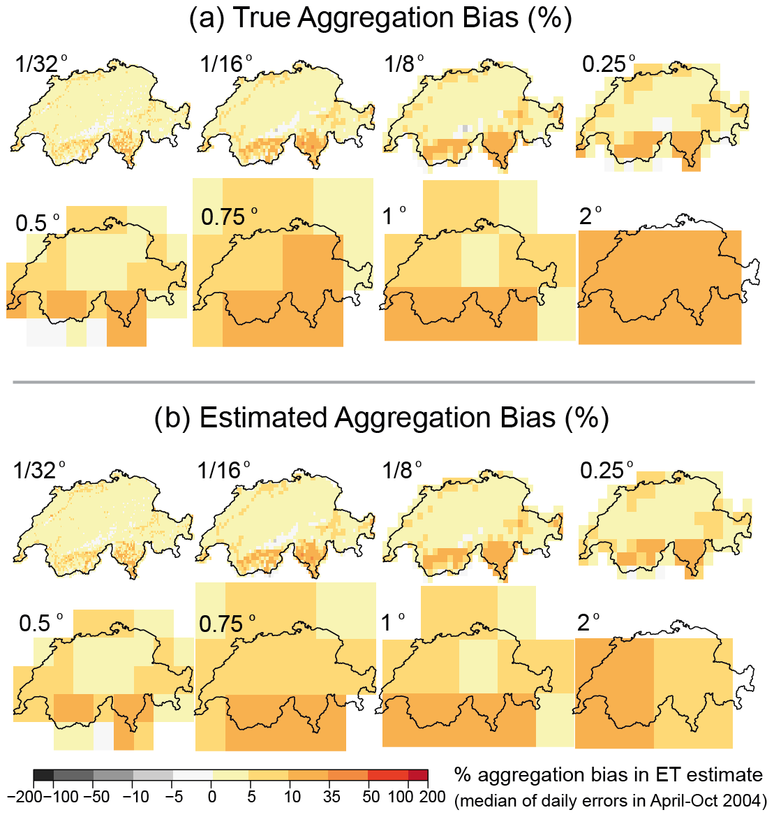
Figure 2(a) True aggregation bias in ET, as calculated by averaging the 500 m resolution ET estimates using fine-resolution input data in Eq. (6), over 1∕32, 1∕16, 1∕8, 0.25, 0.5, 0.75, 1, and 2∘ grid cells across Switzerland. (b) Aggregation bias in ET, as estimated by Eq. (7) from grid-cell-averaged temperature (∘C), soil moisture (ww), net radiation (Rn), their variances at each grid scale, and the covariances of all pairs of variables using the 500 m input data. At finer grid scales, the aggregation bias is more localized and smaller on average. Across Switzerland as a whole, the average aggregation bias becomes smaller as grid scales become finer but never disappears completely.
Using our 500 m input data, we can test how well Eq. (7) estimates the difference between the true average ET and the coarse-resolution modeled ET at each grid scale. We used Eqs. (8)–(14) to calculate the partial derivatives of the GLEAM equations for each grid cell and time step, using the grid-cell-averaged values of the input data. We then multiplied these derivatives by the corresponding variances and covariances among the 500 m input data to obtain bias estimates via Eq. (15) for each grid cell and time step:
where is the true average ET at some grid resolution, is the modeled coarse-resolution ET at the same spatial scale, and the right-hand side is the Taylor expansion estimate of the aggregation bias. We then compared these estimated biases against the true aggregation biases (the difference between the true average ET and the coarse-resolution modeled ET) in the numerical experiment described above. The true bias, in other words, is in Eq. (15), and the estimated bias is the Taylor approximation on the right-hand side.
Figure 2b shows that the aggregation bias estimated by Eq. (15) is generally similar, in both overall magnitude and spatial distribution, to the true aggregation biases calculated by the numerical experiment. This comparison is shown more explicitly in Fig. 3, in which the estimated aggregation bias is compared with the true aggregation bias for each grid cell at each grid scale. Figures 2 and 3 show that Eq. (15) is generally a good predictor of aggregation bias. Both the estimated aggregation biases (Fig. 2) and the true aggregation biases are markedly higher in regions of greater topographic complexity (Fig. S4).

Figure 3Daily estimated aggregation bias in ET estimates (%, median of daily biases in April–October 2004) versus daily true aggregation bias in ET estimates (%, median of daily biases in April–October 2004) at several spatial scales. Estimated aggregation biases are calculated using Eq. (7). True aggregation biases are calculated as differences between the finer-resolution ET estimates from finer-resolution input data, averaged over several spatial scales (average of functions) and ET values calculated from average inputs at each spatial scale (function of averages). The coefficients of determination (R2) between the true and estimated aggregation biases verify the reliability of the Taylor expansion method and Eq. (7) as estimates of the aggregation bias.
2.4 Correcting for aggregation bias
2.4.1 Identifying drivers of aggregation bias
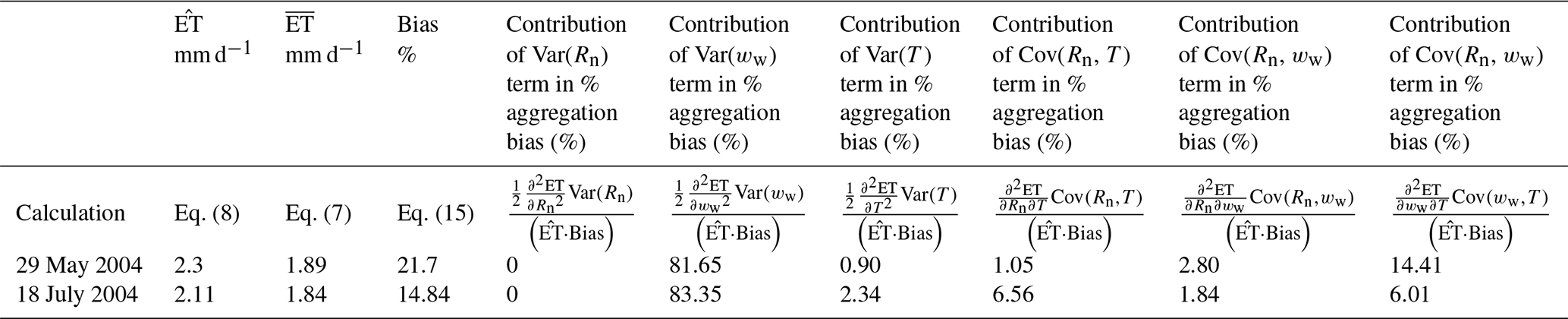
The Taylor expansion in Eq. (15) not only allows one to quantify the aggregation bias; it also allows one to quantify the relative importance of the three input variables (net radiation, soil moisture, and temperature) as drivers of that bias. Each of the terms in Eq. (15) combines a variance or covariance that expresses how variable the input data are and a second derivative that expresses how sensitive the average ET is to that variability. Each of these terms – a derivative multiplied by a variance or covariance – has the same units as ET, and thus they can be directly compared to one another.
Table 1 shows each of the aggregation bias terms, calculated over all of Switzerland for the two arbitrarily chosen days mentioned in Sect. 2.3 (29 May and 18 July 2004). For these two example days, the aggregation bias is clearly dominated by a single term, associated with the variance of soil moisture. The variance in net radiation (Rn) creates no aggregation bias, because GLEAM ET is a linear function of Rn; thus positive and negative deviations from average Rn will increase and decrease ET by exactly offsetting amounts. Similarly, the variance in temperature (T) also results in little aggregation bias, because GLEAM ET increases nearly linearly with T across a wide range of temperature. The covariance terms similarly lead to little aggregation bias. By contrast, the strong curvature in the quadratic dependence of ET on soil moisture (Eq. 6) implies that positive and negative deviations from mean soil moisture will not have offsetting ET effects, and thus that spatial heterogeneity in soil moisture can significantly alter average ET. On most of the days of the year 2004, the soil moisture variance term is the dominant driver of the aggregation bias. However, there are some days in which other factors such as the T and Rn covariance term are the dominant factors.
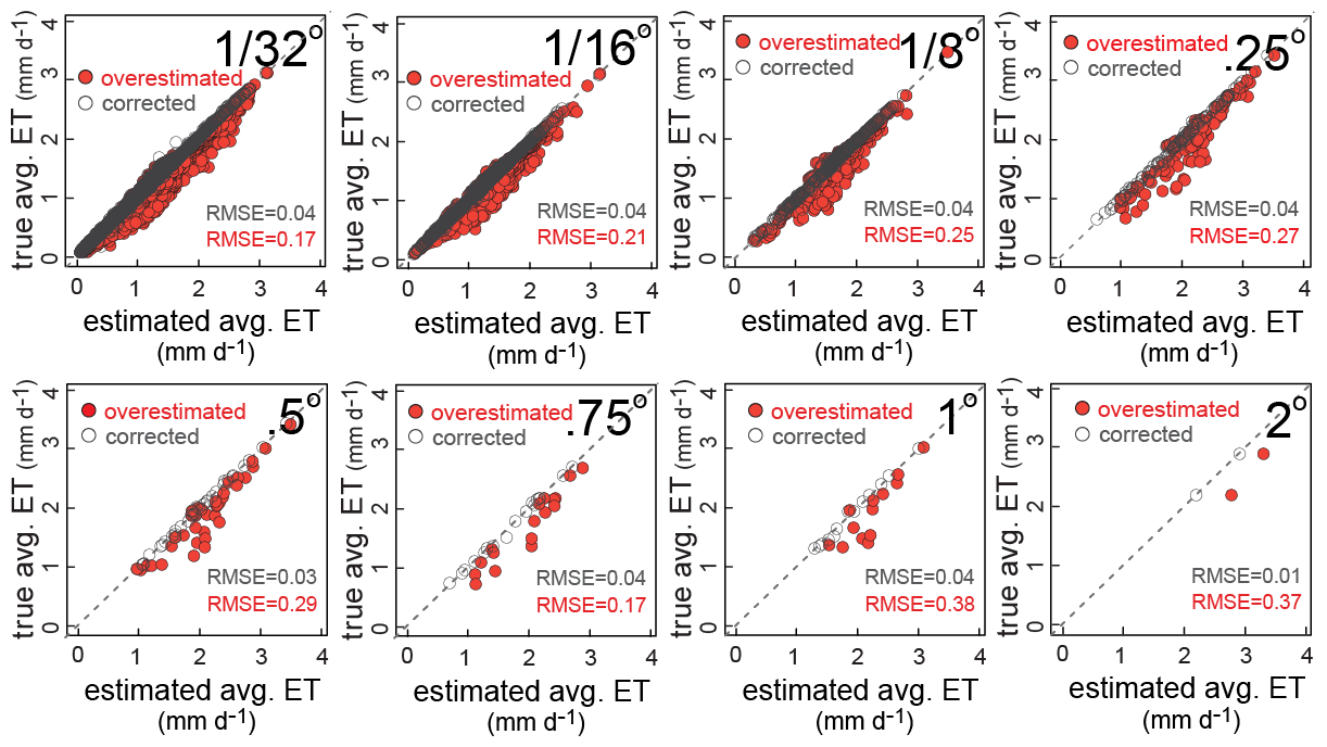
Figure 4Daily estimated ET rates versus true average ET at each grid cell at several different grid scales (example day, 31 May 2004). The solid red symbols demonstrate the relationships between true average ET calculated using fine-resolution data at each grid cell and modeled grid-cell-averaged ET using grid-cell-averaged inputs in Eq. (8), for each grid cell at several different grid scales (overestimated). For comparison, the open symbols show true average versus average ET estimated by the Taylor expansion approach of Eq. (7), which corrects for sub-grid heterogeneity effects using only grid-cell-averaged estimates of the ET drivers and their small-scale variances and covariances (heterogeneity-corrected ET estimates, corrected).
Table 1Relative importance of different ET drivers in aggregation bias estimates (different terms in Eq. 15). Values are calculated for all of Switzerland for the two arbitrarily chosen days (29 May and 18 July 2004). The aggregation bias is dominated by the term associated with the variance of soil moisture for these two example days.
2.4.2 Correcting for aggregation bias using sub-grid closure relationships
The Taylor expansion framework in Eq. (7) can be used not only to diagnose aggregation bias, but also to estimate sub-grid closure relationships that correct for the effects of small-scale heterogeneity. The variance and covariance terms in Eq. (7) express how sub-grid heterogeneity affects average ET at the grid scale, implying that these aggregation bias estimates could be used to improve grid-scale ET estimates, without explicitly modeling ET at high resolutions. This approach could be particularly useful in land surface algorithms that are part of coarser-resolution Earth system models; in such cases it may be much more efficient to evaluate Eqs. (7)–(14) at the coarse grid resolution than to directly evaluate the underlying ET model, Eq. (6), at high resolution. The Taylor expansion approach could also be attractive where we lack spatially explicit high-resolution maps of the ET drivers, but where their variances and covariances can nonetheless be estimated from other sources (i.e., from the variability of topography, mapped soil units, remote sensing data, etc.).
It is beyond our scope here to construct such variance and covariance estimates, but we can illustrate how they could potentially be used. The solid red symbols in Fig. 4 show the relationships between true average ET and modeled grid-cell-averaged ET, for each grid cell (and one example day, 31 May 2004) at several different grid scales. For comparison, the open grey symbols in Fig. 4 show average ET estimated by the Taylor expansion approach of Eq. (7), which corrects for sub-grid heterogeneity effects using only grid-cell-averaged estimates of the ET drivers and their small-scale variances and covariances.
The heterogeneity-corrected ET estimates shown by the open symbols in Fig. 4 cluster much closer to the 1:1 line than the modeled grid-cell-averaged ET values shown by the solid red symbols, suggesting that the Taylor expansion approach may substantially improve estimates of grid-cell-averaged ET. Real-world results may be less clear than those shown in Fig. 4, because the heterogeneity-corrected ET estimates (the open symbols in Fig. 4) are calculated using exact values for the variances and covariances of the ET drivers within each grid cell, and in real-world cases these variances and covariances will not be known precisely. Figure 4 nonetheless demonstrates the potential value of knowing, or being able to estimate, those variances and covariances. Efforts to determine those variances and covariances can be focused on the terms that matter the most, if one can identify the main drivers of aggregation bias using the methods described in Sect. 2.2 above.
Averaging over spatially heterogeneous ET drivers leads to substantial aggregation biases in ET flux estimates from a typical mechanistic large-scale land surface model. This aggregation bias arises from the inherent nonlinearities in evapotranspiration processes, coupled with the inherent spatial heterogeneity in the driving factors. The joint effects of these nonlinearities and heterogeneities can be estimated using second-order Taylor expansions of the governing equations. Using Switzerland as a test case, we have shown that median aggregation biases of 10 %–35 % are common, even at grid scales substantially smaller than those typically used in land surface models (Fig. 2). These biases can be much larger for individual days (Figs. S2 and S3) and potentially have substantial consequences for water and energy flux estimates in land surface models and consequently for temperature predictions in coupled models. The overestimated evaporative fluxes would lead to overestimated latent heat fluxes and underestimated sensible heat fluxes, and thus potentially to underestimates of expected temperature increases in a changing climate. Unrealistically high evaporation estimates lead to cooler modeled temperatures and wetter modeled climates. Correcting for the aggregation bias in ET fluxes would lead to reduced evaporative cooling and increased atmospheric heating via sensible heat flux.
In coupled Earth system models, ET fluxes influence how surface temperature, net radiation, and soil moisture evolve through time and thus influence future values of ET. The analyses shown in Figs. 2–4 are based on static values for each day and thus do not account for the propagation of aggregation biases forward through time. Estimating the consequences of aggregation biases for dynamic modeling would require fully coupled Earth system model simulations rather than the single ET algorithm analyzed here. In a dynamic model, the Taylor expansion approach can potentially be used to correct for aggregation biases in each time step, using statistical models for the variances and covariances of the ET drivers. Thus, estimating aggregation biases in a dynamic model would not require explicitly simulating sub-grid heterogeneity at every time step. Correcting for aggregation biases at each modeling time step would prevent them from propagating further into future time steps or into the partitioning of future water and energy fluxes at the land surface. The present paper does not illustrate this dynamic correction for aggregation biases but establishes the theoretical framework for it.
The purpose of our analysis was to demonstrate how aggregation bias due to spatial heterogeneity can be quantified (Sect. 2.2 and 2.3), how its dominant drivers can be identified (Sect. 2.4.1), and how its effects can be efficiently corrected for, using sub-grid closure relationships (Sect. 2.4.2). For this demonstration, we chose GLEAM as an illustrative example and Switzerland as a topographically complex case study where high-resolution data on the ET drivers are available. Applications of this approach to more complex land surface models may require calculating the necessary derivatives (see Eq. 7) numerically rather than analytically, and applications where high-resolution data are unavailable may require statistically estimating the variances and covariances among the drivers of ET, based on their relationships with topography, soil types, land cover, etc. Using the approach outlined here, one can account for the effects of sub-grid heterogeneity without explicitly modeling ET at fine spatial resolution, which could be impractical due to computational costs or impossible due to a lack of fine-resolution input data.
In our analysis, spatial heterogeneity in soil moisture emerged as the dominant driver of aggregation bias in ET estimates. Particularly if this result can also be confirmed in other regions and climates, it points to the importance of improving our understanding of spatial patterns of soil moisture and what controls them. The lower topographic curvature of coarsely gridded landscapes can lead models to predict higher soil moisture at coarser grid scales (Kuo et al., 1999); higher soil moisture at larger grid scales would lead to even higher modeled values of ET, beyond the effects of the aggregation biases analyzed here. Soil moisture may also be substantially influenced by lateral subsurface transfers of water, which are ignored in our analysis and are also ignored by many land surface models. Overlooking lateral transfers could potentially bias ET estimates in large-scale land surface models (Fan et al., 2019), but this is beyond the scope of the present study.
Temperature data are an interpolation of MeteoSwiss data after Viviroli et al. (2009) and are originally from archive data of MeteoSwiss ground level monitoring networks. However, the acquired data may not be used for commercial purposes (e.g., by passing on the data to third parties or by publishing them on the internet). As a consequence, we cannot offer direct access to the data used in this study. Daily soil moisture saturation, net radiation, and temperature data over Switzerland at a 500 m resolution for the year 2004 can be retrieved from EnviDat at https://doi.org/10.16904/envidat.176 (Rouholahnejad Freund et al., 2020b).
The supplement related to this article is available online at: https://doi.org/10.5194/hess-24-5015-2020-supplement.
ERF and JWK designed the study. ERF ran the analysis. MZ provided the soil moisture simulations and contributed to the discussions. ERF and JWK wrote the paper.
The authors declare that they have no conflict of interest.
We thank Ying Fan Reinfelder for numerous insightful discussions and for helpful comments on the manuscript. Elham Rouholahnejad Freund acknowledges support from the Swiss National Science Foundation (SNSF) under grant no. P2EZP2_162279.
This research has been supported by the Swiss National Science Foundation (grant no. P2EZP2_162279).
This paper was edited by Anke Hildebrandt and reviewed by two anonymous referees.
Beven, K. J.: The holy grail of scientific hydrology: Qt=(S, R, Δt)A as closure, Hydrol. Earth Syst. Sci., 10, 609–618, https://doi.org/10.5194/hess-10-609-2006, 2006.
Beven, K. J. and Cloke, H. L.: Comment on “Hyperresolution global land surface modeling: Meeting a grand challenge for monitoring Earth's terrestrial water” by Eric F. Wood et al., Water Resour. Res., 48, W01801, https://doi.org/10.1029/2011WR010982, 2012.
Boone, A. and Wetzel, O. J.: A simple scheme for modeling sub-grid soil texture variability for use in an atmospheric climate model, J. Meteorol. Soc. Jpn., 77, 317–333, https://doi.org/10.2151/jmsj1965.77.1B_317, 1998.
Brunner, M. I., Liechti, K., and Zappa, M.: Extremeness of recent drought events in Switzerland: dependence on variable and return period choice, Nat. Hazards Earth Syst. Sci., 19, 2311–2323, https://doi.org/10.5194/nhess-19-2311-2019, 2019.
Brunt, D.: Physical and dynamical meteorology, 2nd Edn., Cambridge University Press, Cambridge, 428 pp., 1952.
Brutsaert, W.: Evaporation into the atmosphere, Springer Science and Business Media, Dordrecht, https://doi.org/10.1007/978-94-017-1497-6, 1984.
El Maayar, M. and Chen, J. M.: Spatial scaling of evapotranspiration as affected by heterogeneities in vegetation, topography, and soil texture, Remote Sens.f Environ., 102, 33–51, https://doi.org/10.1016/j.rse.2006.01.017, 2006.
Ershadi A., McCabe, M. F., Evans, J. P., and Walker, J. P.: Effects of spatial aggregation on the multi-scale estimation of evapotranspiration, Remote Sens. Environ., 131, 51–62, https://doi.org/10.1016/j.rse.2012.12.007, 2013.
Fan, Y., Clark, M., Lawrence, D. M., Swenson, S., Band, L. E., Brantley, S. L., Brooks, P. D., Dietrich, W. E., Flores, A., Grant, G., Kirchner, J. W., Mackay, D. S., McDonnell, J. J., Milly, P. C. D., Sullivan, P. L., Tague, C., Ajami, H., Chaney, N., Hartmann, A., Hazenberg, P., McNamara, J., Pelletier, J., Perket, J., Rouholahnejad-Freund, E., Wagener, T., Zeng, X., Beighley, E., Buzan, J., Huang, M., Livneh, B., Mohanty, B. P., Nijssen, B., Safeeq, M., Shen, C., van Verseveld, W., Volk, J., and Yamazaki, D.: Hillslope hydrology in global change research and Earth system modeling, Water Resour. Res., 55, 1737–1772, https://doi.org/10.1029/2018WR023903, 2019.
Gash, J. H. C.: an analytical model of rainfall interception by forests, Q. J. Roy. Meteorol. Soc. 105, 43–55, https://doi.org/10.1002/qj.49710544304, 1979.
Gash, J. H. C. and Stewart, J. B.: The evaporation from Thetford Forest during 1975, J. Hydrol., 35, 385–396, 1977.
Giorgi, F.: An Approach for the Representation of Surface Heterogeneity in Land Surface Models. Part I: Theoretical Framework, Mon. Weather Rev., 125, 1885–1899, https://doi.org/10.1175/1520-0493(1997)125<1885:AAFTRO>2.0.CO;2, 1997.
Giorgi, F. and Avissar, R.: Representation of heterogeneity effects in Earth system modeling: Experience from land surface modeling, Rev. Geophys., 35, 413–437, https://doi.org/10.1029/97RG01754, 1997.
Greve, P., Orlowsky, B., Mueller, B., Sheffield, J., Reichstein, M., and Seneviratne, S. I.: Global assessment of trends in wetting and drying over land, Nat. Geosci., 7, 716–721, 2014.
Hong, S. H., Hendrickx, J. M. H., and Borchers, B.: Up-scaling of SEBAL derived evapotranspiration maps from Landsat (30 m) to MODIS (250 m) scale, J. Hydrol., 370, 122–138, https://doi.org/10.1016/j.jhydrol.2009.03.002, 2009.
Huang, X., Rhoades, A. M., Ullrich, P. A., and Zarzycki, C. M.: An evaluation of the variable-resolution-CESM for modeling California's climate, J. Adv. Model. Earth Syst., 8, 345–369, https://doi.org/10.1002/2015MS000559, 2016.
Jasechko, S., Sharp, Z. D., Gibson, J. J., Birks, S. J., Yi, Y., and Fawcett, P. J.: Terrestrial water fluxes dominated by transpiration, Nature, 496, 347–350, https://doi.org/10.1890/ES13-00391.1, 2013.
Kuo, W. L., Steenhuis, T. S., McCulloch, C. E., Mohler, C. L., Weinstein, D. A., DeGloria, S. D., and Swaney, D. P.: Effect of grid size on runoff and soil moisture for a variable-source-area hydrology model, Water Resour. Res., 35, 3419–3428, https://doi.org/10.1029/1999WR900183, 1999.
Martens, B., Miralles, D. G., Lievens, H., van der Schalie, R., de Jeu, R. A. M., Fernández-Prieto, D., Beck, H. E., Dorigo, W. A., and Verhoest, N. E. C.: GLEAM v3: satellite-based land evaporation and root-zone soil moisture, Geosci. Model Dev., 10, 1903–1925, https://doi.org/10.5194/gmd-10-1903-2017, 2017.
McCabe, M. and Wood, E.: Scale influences on the remote estimation of evapotranspiration using multiple satellite sensors, Remote Sens. Environ., 105, 271–285, https://doi.org/10.1016/j.rse.2006.07.006, 2006.
Miralles, D. G., Holmes, T. R. H., De Jeu, R. A. M., Gash, J. H., Meesters, A. G. C. A., and Dolman, A. J.: Global land-surface evaporation estimated from satellite-based observations, Hydrol. Earth Syst. Sci., 15, 453–469, https://doi.org/10.5194/hess-15-453-2011, 2011.
Miralles, D. G., van den Berg, M. J., Gash, J. H., Parinussa, R. M., de Jeu, R. A. M., Beck, H. E., Holmes, T. R. H., Jiménez, C., Verhoest, N. E. C., Dorigo, W. A., Teuling, A. J., and Dolman, A. J.: El Niño–La Niña cycle and recent trends in continental evaporation, Nat. Clim. Change, 4, 122–126, https://doi.org/10.1038/NCLIMATE2068, 2013.
Miralles, D. G., Teuling, A. J., van Heerwaarden, C. C., and Vilà-Guerau de Arellano, J.: Mega-heatwave temperatures due to combined soil desiccation and atmospheric heat accumulation, Nat. Geosci., 7, 345–349, https://doi.org/10.1038/NGEO2141, 2014.
Monteith, J. L.: Evaporation and environment, the state of and movement of water in living organisms, P. Soc. Exp. Biol., 19, 205–234, https://doi.org/10.1002/qj.49710745102, 1965.
Monteith, J. L. and Unsworth, M. H.: Principles of Environmental Physics, Edward Arnold, London, 1990.
Mueller, B., Hirschi, M., Jimenez, C., Ciais, P., Dirmeyer, P. A., Dolman, A. J., Fisher, J. B., Jung, M., Ludwig, F., Maignan, F., Miralles, D. G., McCabe, M. F., Reichstein, M., Sheffield, J., Wang, K., Wood, E. F., Zhang, Y., and Seneviratne, S. I.: Benchmark products for land evapotranspiration: LandFlux-EVAL multi-data set synthesis, Hydrol. Earth Syst. Sci., 17, 3707–3720, https://doi.org/10.5194/hess-17-3707-2013, 2013.
Murray, F. W.: On the computation of saturation vapor pressure, J. Appl. Meteorol., 6, 203–204, https://doi.org/10.1175/1520-0450(1967)006<0203:OTCOSV>2.0.CO;2, 1967.
Orth, R., Staudinger, M., Seneviratne, S. I., Seibert, J., and Zappa, M.: Does model performance improve with complexity? A case study with three hydrological models, J. Hydrol., 523, 147–159, https://doi.org/10.1016/j.jhydrol.2015.01.044, 2015.
Penman, H. L.: Natural evaporation from open water, bare soil, and grass, P. Roy. Soc. Lond. A, 193, 120–146, 1948.
Priestley, C. H. B. and Taylor, R. J.: On the assessment of surface heat flux and evaporation using large-scale parameters, Mon. Weather Rev., 100, 81–92, https://doi.org/10.1175/1520-0493(1972)100<0081:otaosh>2.3.co;2, 1972.
Rastetter, E. B., King, A. W., Cosby, B. J., Hornberger, G. M., O'Neill, R. V., and Hobbie, J. E.: Aggregating Fine-Scale Ecological Knowledge to Model Coarser-Scale Attributes of Ecosystems, Ecol. Appl., 2, 55–70, https://doi.org/10.2307/1941889, 1992.
Rauscher, S. A., Coppola, E., Piani, C., and Giorgi, F.: Resolution effects on regional climate model simulations of seasonal precipitation over Europe, Clim. Dynam., 35, 685–711, https://doi.org/10.1007/s00382-009-0607-7, 2010.
Ringler, T., Ju, L., and Gunzburger, M.: A multiresolution method for climate system modeling: Application of spherical centroidal Voronoitessellations, Ocean Dynam., 58, 475–498, https://doi.org/10.1007/s10236-008-0157-2, 2008.
Rouholahnejad Freund, E. and Kirchner, J. W.: A Budyko framework for estimating how spatial heterogeneity and lateral moisture redistribution affect average evapotranspiration rates as seen from the atmosphere, Hydrol. Earth Syst. Sci., 21, 217–233, https://doi.org/10.5194/hess-21-217-2017, 2017.
Rouholahnejad Freund, E., Fan, Y., and Kirchner, J. W.: Global assessment of how averaging over spatial heterogeneity in precipitation and potential evapotranspiration affects modeled evapotranspiration rates, Hydrol. Earth Syst. Sci., 24, 1927–1938, https://doi.org/10.5194/hess-24-1927-2020, 2020a.
Rouholahnejad Freund, E., Zappa, M., and Kirchner, J. W.: Daily 500 m gridded net radiation and soil moisture for Switzerland, 2004, EnviDat, https://doi.org/10.16904/envidat.176, 2020b.
Shrestha, P., Sulis, M., Simmer, C., and Kollet, S.: Effects of horizontal grid resolution on evapotranspiration partitioning using TerrSysMP, J. Hydrol., 557, 910–915, https://doi.org/10.1016/j.jhydrol.2018.01.024, 2018.
Skamarock, W. C., Klemp, J. B., Duda, M. G., Fowler, L. D., Park, S.-H., and Ringler, T. D.: A multiscale nonhydrostatic atmospheric model using centroidal Voronoi tesselations and C-grid staggering, Mon. Weather Rev., 140, 3090–3105, https://doi.org/10.1175/MWR-D-11-00215.1, 2012.
Speich, M. J. R., Bernhard, L., Teuling, A. J., and Zappa, M.: Application of bivariate mapping for hydrological classification and analysis of temporal change and scale effects in Switzerland, J. Hydrol., 523, 804–821, https://doi.org/10.1016/j.jhydrol.2015.01.086, 2015.
Stanghellini, C., Transpiration of Greenhouse Crops. PhD thesis, Wageningen University, Wageningen, The Netherlands, 1987.
Tetens, O.: Über einige meteorologische Begriffe, Z. Geophys., 6, 297–309, 1930.
Viviroli, D., Zappa, M., Gurtz, J., and Weingartner, R.: An introduction to the hydrological modelling system PREVAH and its pre- and post-processing-tools, Environ. Model. Softw., 24, 1209–1222, https://doi.org/10.1016/j.envsoft.2009.04.001, 2009.
Zappa, M. and Gurtz, J.: Simulation of soil moisture and evapotranspiration in a soil profile during the 1999 MAP-Riviera Campaign, Hydrol. Earth Syst. Sci., 7, 903–919, https://doi.org/10.5194/hess-7-903-2003, 2003.
Zarzycki, C. M., Levy, M. N., Jablonowski, C., Overfelt, J. R., Taylor, M. A., and Ullrich, P. A.: Aquaplanet experiments using CAM's variable-resolution dynamical core, J. Climate, 27, 5481–5503, https://doi.org/10.1175/JCLI-D-14-00004.1, 2014.