Efficient screening of groundwater head monitoring data for anthropogenic effects and measurement errors

Groundwater levels are monitored by environmental agencies to support the sustainable use of groundwater resources. For this purpose continuous and spatially comprehensive monitoring in high spatial and temporal resolution is desired. This leads to large datasets that have to be checked for quality and analysed to distinguish local anthropogenic influences from natural variability of the groundwater level dynamics at each well. Both technical problems with the measurements as well as local anthropogenic influences can lead to local anomalies in the hydrographs. We suggest a fast and efficient screening method for the identification of well-specific peculiarities in hydrographs of groundwater head monitoring networks. The only information required is a set of time series of groundwater heads all measured at the same instants of time. For each well of the monitoring network a reference hydrograph is calculated, describing expected “normal” behaviour at the respective well as is typical for the monitored region. The reference hydrograph is calculated by multiple linear regression of the observed hydrograph with the “stable” principal components (PCs) of a principal component analysis of all groundwater head series of the network as predictor variables. The stable PCs are those PCs which were found in a random subsampling procedure to be rather insensitive to the specific selection of the analysed observation wells, i.e. complete series, and to the specific selection of measurement dates. Hence they can be considered to be representative for the monitored region in the respective period. The residuals of the reference hydrograph describe local deviations from the normal behaviour. Peculiarities in the residuals allow the data to be checked for measurement errors and the wells with a possible anthropogenic influence to be identified. The approach was tested with 141 groundwater head time series from the state authority groundwater monitoring network in northeastern Germany covering the period from 1993 to 2013 at an approximately weekly frequency of measurement.

1 Introduction

Sustainable management of groundwater resources aims to ensure that the abstraction of groundwater does not exceed groundwater recharge over the long term (e.g. Gleeson et al., 2012). This resonates in the Water Framework Directive of the European Union which aims to achieve and maintain a good status of groundwater quantity; it includes the obligation to monitor the temporal development of groundwater storage with sufficient spatial and temporal resolution to be able to distinguish between anthropogenic influences and natural variability (EU, 2000).

In practice declining trends in observed groundwater head time series often serve as a first indication for anthropogenic effects. However, declining trends in hydrological systems do not necessarily imply anthropogenic influence, but they might rather be indications of naturally occurring long-term persistence (Hurst, 1951; Mandelbrot and Van Ness, 1968; Mandelbrot and Wallis, 1969) induced for example by the natural fluctuation of climatic drivers (e.g. Koutsoyiannis, 2006). Thus continuity of hydrologic records for more than “just” a few decades is mandatory to incorporate this issue in water management (Hirsch, 2011). This holds in particular for groundwater monitoring due to the much more pronounced filtering of short-term fluctuations in the subsurface compared to precipitation, soil moisture, or streamflow (Skøien et al., 2003).

Thus, the sustainable management of groundwater resources requires a spatially differentiated and comprehensive monitoring of the groundwater level covering its temporal development continuously over decades which leads to large datasets. Checking the data quality at the wells of a spatially comprehensive network can be very time consuming. Measurement errors as well as local anthropogenic influences lead to anomalies at individual sites. Thus, local anomalies in the hydrographs can serve as an indication for both aspects. That requires a reference either in the form of observed hydrographs measured at specific observation wells which are considered representative for undisturbed behaviour typical for the region (e.g. Winter et al., 2000; Gangopadhyay et al., 2001) or in the form of some kind of modelled regional reference hydrograph. Here, we focus on the second case.

One option is to apply a physically based model for that purpose. Depending on the characteristics of the region and the level of model complexity, the amount of data required can be large (cf. discussion in Coppola et al., 2003). A non-exhaustive list of typical basic requirements includes climatological data to drive the model, data on the hydraulic properties of the subsurface which could comprise various aquifers, data on land use or time series of water abstraction, etc. That information is required in a spatially distributed manner. In many cases, the monitoring effort, the effort to set up the model, the complexity of the model, and the demand on data are substantial obstacles for environmental authorities or consultants at larger spatial scales.

Consequently, in practice some model parameters will serve during calibration as a surrogate for missing data. For example, Wriedt (2017) calculated a “theoretical climatic hydrograph” for each observation well in a monitoring network by fitting the monthly climatic water balance to the observed groundwater hydrograph using a damping and a translation factor. Here, the fitting of the damping and the translation factor compensated for missing information on different properties of the analysed groundwater system like different substrates, flow paths, etc.

Another option is to fit empirical models based on the relationships between easy-to-obtain independent variables and the observed water level. This has been performed for example by means of multiple linear regression (Hodgson, 1978), artificial neural networks (Coulibaly et al., 2001; Coppola et al., 2003), the combination of an artificial neural network and a linear autoregressive model with exogenous input (Wunsch et al., 2018), or different other approaches from the field of artificial intelligence employing methods like adaptive neuro-fuzzy inference systems, genetic programming, support vector machines, or hybrid models such as wavelet–artificial intelligence models (Rajaee et al., 2019). Others applied time series models like the predefined impulse response function in continuous time models (Von Asmuth et al., 2008), mixed models which combine deterministic fixed effects models with statistical random effects models (Marchant et al., 2016), or the combination of different methods from the fields of exploratory data analysis, information theory, and machine learning (Sahoo et al., 2017). Those data-driven approaches make efficient use of the available data and are therefore recommended as a relatively cost- and time-efficient way to model groundwater level in areas with limited data (Hodgson, 1978; Coulibaly et al., 2001; Coppola et al., 2003). Another benefit is that the respective models can easily be updated once new measurements or additional variables become available (Coppola et al., 2003).

Here, we suggest to derive local reference time series based on a principal component analysis (PCA) of a set of monitored time series. This approach does not require any other data than the time series of water level all measured at same instants of time. PCA is one of the most established, fastest and computationally cheapest statistical approaches to summarize the spatiotemporal variability of a set of spatially distributed time series. Based on the linear correlation structure of the dataset linearly independent principal components (PCs) are derived. Each PC is associated with one characteristic spatiotemporal pattern. Except for being fast and computationally very cheap, PCA is readily implemented in most of the common statistical software packages.

In analogy to climatology (e.g. Richman, 1986), the spatiotemporal patterns of the PCs have been used for a long time in hydrology as a compact description of the dominant modes of hydrological variability in a region. Pioneering studies used it to describe dominant modes of streamflow variability in the European USSR (Smirnov, 1972, 1973), the USA and southern Canada (Bartlein, 1982), the USA alone (Lins, 1985a, b, 1997), and different regions of Sweden (Gottschalk, 1985). The leading PCs were used in combination with cluster analysis for the classification of streamflow (Hannah et al., 2000) and groundwater (Triki et al., 2014) hydrographs into groups with similar dynamics, which allowed for example for reducing the effort of modelling of all the time series in a groundwater monitoring network to a few representative hydrographs (Upton and Jackson, 2011). These approaches have to be distinguished from using PCs for the identification of prevailing processes or functional relationships (e.g. Longuevergne et al., 2007; Lewandowski et al., 2009; Hohenbrink et al., 2016), which is beyond the scope of this paper.

To our knowledge, the application of PCA-based approaches in the context of compact description of hydrological variability focussed so far mainly on the leading PCs, that is, the main modes of hydrological variability on the scale of the analysed dataset, like the main regional spatiotemporal patterns in a monitoring network. For example, Smirnov (1973) used the leading PCs for filtering small-scale disturbances from the large-scale patterns of long-period streamflow fluctuations in the European USSR. In groundwater monitoring, the leading PCs were used for example in the evaluation of groundwater monitoring networks to identify the observation wells which were most representative for the analysed region (Winter et al., 2000; Gangopadhyay et al., 2001).

In this study, we used the leading principal components of a set of groundwater head time series of a large-scale monitoring network to decompose the observed hydrographs into a reference part and a residual part for each site separately. The reference hydrograph of an observation well describes the expected “normal” behaviour at that well, i.e. the part of the observed hydrograph which is considered typical for the monitored region. It is determined by multiple linear regression of the observed hydrograph with the “stable” PCs as predictor variables. The stable PCs are determined by comparing the results of a series of PCAs which were performed with different randomly selected subsets of the complete dataset. The subdatasets were derived in the spatial domain as random selections of the observation wells, i.e. complete series, and in the temporal domain as random selections of the measurement dates. Those PCs that turned out to be rather insensitive to the specific selection of analysed wells and measurement dates were defined as sufficiently stable and considered to be representative for the monitored region in the analysed period. The residual part of the hydrograph depicts the local deviations from the normal behaviour at the respective observation well, which is then analysed for peculiarities pointing to technical problems or anthropogenic effects. Other applications of the reference hydrograph, like gap filling in series which were not included in the PCA, are shortly discussed. In contrast to other PCA applications this approach does neither require any interpretation of the leading PCs nor any explicit spatial analysis. The approach was tested with 141 groundwater head time series of the authority's groundwater monitoring network of the German federal state of Mecklenburg-Vorpommern covering the period from 1993 to 2013 in an approximately weekly resolution.

2 Data

2.1 Study region

The federal state of Mecklenburg-Vorpommern is located in the northeast of Germany (Fig. 1), covering an area of 23 214 km² (Statistikportal, 2018). The hydrogeological structure in the area consists of several “regional aquifer systems” of Pleistocene origin that are considered to be generally hydraulically separated (Manhenke et al., 2001). The term regional aquifer system describes a system of aquifers of different stratigraphy which are hydraulically connected (Manhenke et al., 2001). Those were formed during different periods of glaciation. Thus, the stratigraphy, or the sequence of stratigraphies, within one aquifer system is not the same everywhere (Manhenke et al., 2001). The water management in the region is based on the aquifer systems and not on single aquifers.

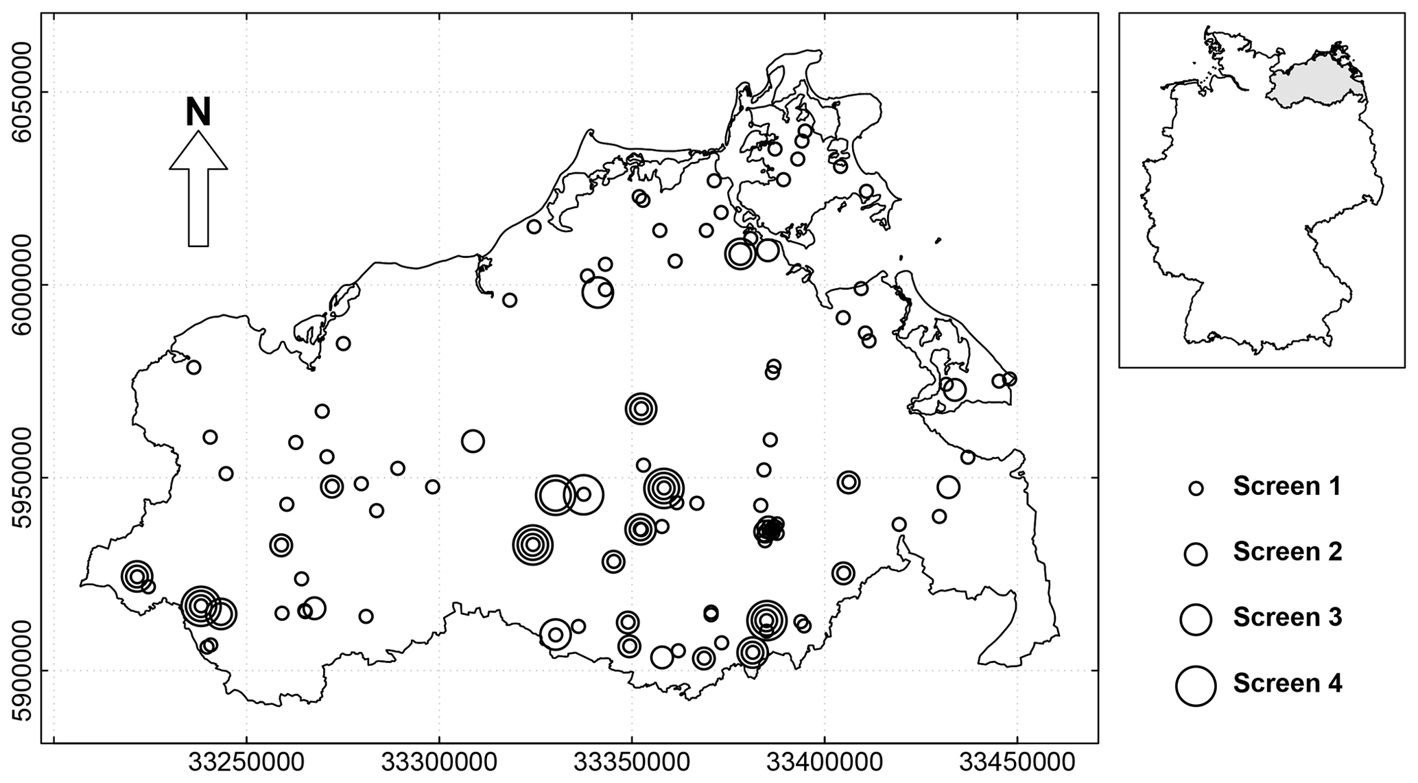
Figure 1 Map of the study area and the selection of groundwater observation wells (N=141) in the federal state of Mecklenburg-Vorpommern (highlighted by grey shading in the inset map). The administrative borders of Germany and of the federal state of Mecklenburg-Vorpommern were obtained from GADM (2017).

Single aquifers can be horizontally as well as vertically separated. The aquifers consist mainly of sandy and gravelly sediments; the intermediate aquitards consist mainly of till. The Pleistocene sediments usually overlie Tertiary sediments and can comprise more than 100 m. Within the Tertiary sediments the Rupelian clay layer hydraulically separates the underlying saline Tertiary groundwater from the fresh groundwater (Manhenke et al., 2001). However, at some locations upwelling salty groundwater reaches the surface (compare LUNG, 1984, and Fig. 2.11-6 in Martens and Wichmann, 2007), indicating that the hydraulic separation of the regional aquifer systems is not complete everywhere.

Groundwater in Mecklenburg-Vorpommern is monitored by the federal State Agency for Environment, Nature Conservation and Geology (LUNG). Monitoring comprised the uppermost three regional aquifer systems, but not all of them are contiguous (Hennig et al., 2002). In addition to the regional aquifer systems, in some areas shallow local aquifers with an extent of usually a few square kilometres, occasionally more than 100 km², have been identified and are monitored as well (Hilgert and Hennig, 2017). These local aquifers are not strictly hydraulically decoupled from the regional aquifer systems, but their hydraulic connection is inhibited (Hilgert and Hennig, 2017). A mean annual groundwater recharge of +122.3 mm for the whole of Mecklenburg-Vorpommern was estimated for the years 1971 to 2000 by Hilgert (2009) based on the work of Hennig and Hilgert (2007). A map of the spatial distribution of the mean annual groundwater recharge is provided by the LUNG (LUNG, 2009).

2.2 Groundwater head data and preprocessing

Groundwater level data were available for 583 observation wells in the monitoring network of the LUNG. In general, the dataset covered a range of different monitoring periods. The mean length of measurement record was approximately 19.9 years. At some wells monitoring started as early as 1953.

For this study, we selected those 141 wells which were continuously monitored during the 20-year period from 1 November 1993 to 22 October 2013 (Fig. 1). All 141 groundwater head series were checked for quality before by the LUNG. The analysed dataset comprised only those time series which were considered to be without any direct anthropogenic effects or measurement errors. During the monitoring period the state agency aimed to take measurements consistently on the 1st, 8th, 15th and 22nd day of the month. Exceptions from this rule appeared for eight series (Fig. S1 in the Supplement). Bi-weekly readings were conducted from the beginning of the monitoring period at two wells until November 2005 and at one well until December 2006. Monthly readings were conducted from the beginning of the monitoring period at two wells until November 2007, at one well until September 2001, and at another well until December 2003. At one well the reading interval was changed to monthly readings in May 2002 and continued so until the end of the monitoring period. The variety of days between subsequent readings is shown for each series in Fig. S2. The mean, minimum, and maximum of all 141 series' mean measurement intervals were 5.3, 1.5, and 13.6 d. The mean, minimum, and maximum of all 141 series' maximum time gaps between subsequent measurement dates were 24.3, 10, and 88 d. All data gaps were linearly interpolated. Subsequently, regular quasi-weekly time series were generated by selecting readings of the 1st, 8th, 15th, and 22nd of each month of the 20-year period. This resulted in a set of 141 groundwater head time series each with readings at the same 960 quasi weekly measurement dates. Thus, the last “quasi-week” exhibited different lengths for the different months.

The observation wells were irregularly distributed (Fig. 1). This is a consequence of the mission of the state agency to monitor possible anthropogenic influences on groundwater level, thus focusing on more densely populated areas. At 35 sites wells were screened at different depths. Distances between the closest observation wells ranged from 0 km, at the sites with several wells, to 20.2 km, with a mean distance between closest wells of 3.4 km. At each site, the screens were numbered from the surface downwards (Fig. 1). Different numbers of the screens do not necessarily imply different aquifers. Comparing two observation wells of different sites, a higher screen number does not imply that the distance of the screen or of the water level to the surface is larger as well (Fig. 2). The mean depth to groundwater, measured as distance of the groundwater head to the cap of the well head during the observation period, ranged from 0.65 to 30.96 m, with a mean of 6.30 m and a standard deviation of 5.36 m. The distribution of monitored mean depths to groundwater was heavily skewed towards smaller depths (Fig. 2). Due to the complex hydrogeological setting, the capture zones of the wells usually are not known with sufficient detail.

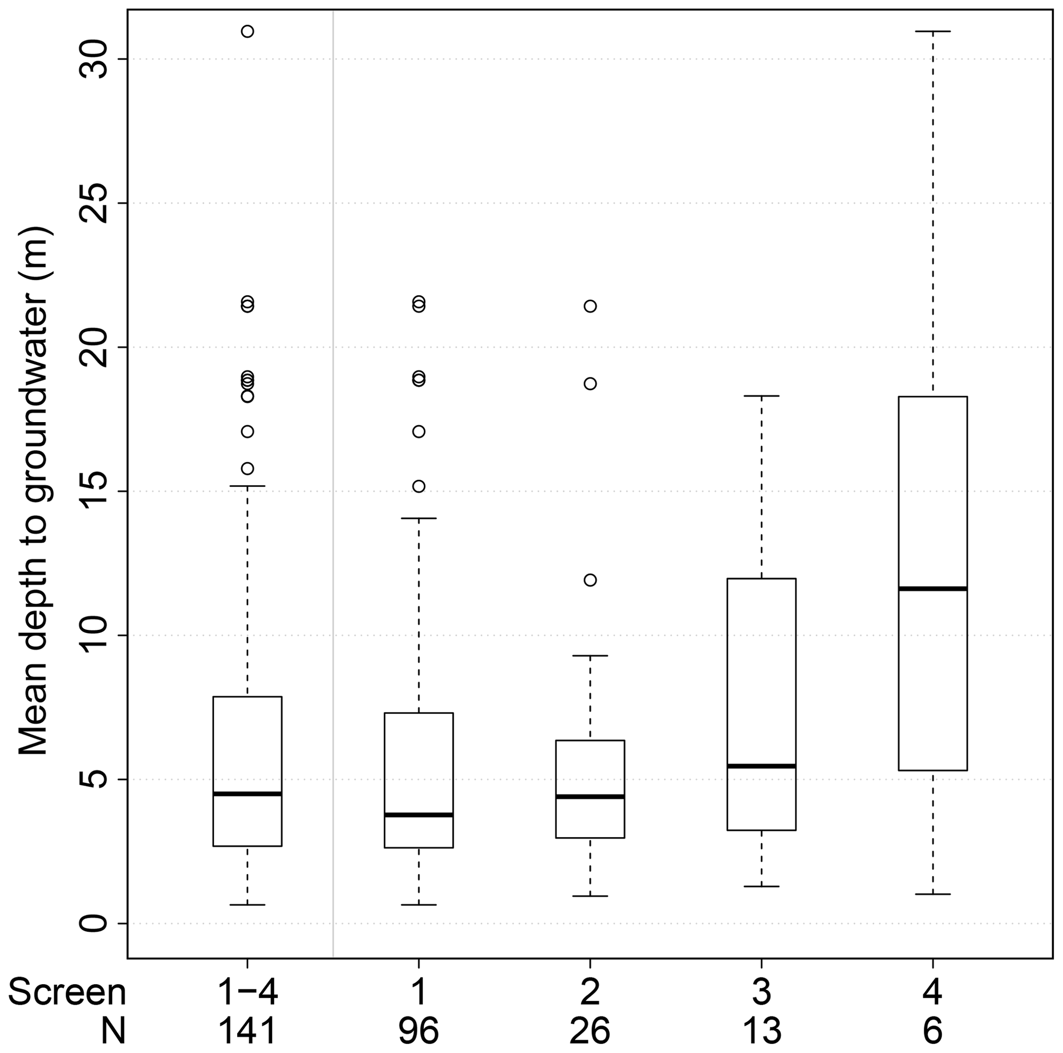
Figure 2 Mean depths to groundwater at the observation wells in metres of the complete set of series and separately for each screen number.

As a rough approximation of the autocorrelation of the time series in spite of the weekly sampling intervals not being completely regular, the correlation of the series with itself shifted by one time step were assessed, yielding a correlation coefficient of r=0.97 with a standard deviation of 0.04. The correlation in the spatial domain between the series of the closest adjacent observation wells was substantially weaker with a mean correlation of r=0.76 and exhibited substantially larger variability with a standard deviation of 0.24.

3 Methods

3.1 Principal component analysis

The spatiotemporal variability in the groundwater head monitoring network was summarized with linearly independent principal components determined by principal component analysis. The PCs are derived by an eigenvalue decomposition of the covariance matrix of the analysed set of variables, that is, the observed groundwater head series. To achieve equal weighting of all series, we applied PCA to the z-scaled groundwater head series, thus each series was scaled to a mean of zero and a standard deviation of one. This corresponds to performing PCA with the correlation matrix of the groundwater head series.

Each PC consists of an eigenvalue, eigenvector (loadings), and scores. The size of the eigenvalue of a PC in relation to the sum of all eigenvalues of all PCs corresponds to the share of variance in the dataset that is assigned to that PC. The loadings are the weights in the linear combination of the analysed variables, here the z-scaled groundwater head series, to calculate the scores of the PCs.

In this study, the analysed dataset consisted of a set of time series all covering the same period and exhibiting the same dates. Thus, the scores of the PCs are times series with the same dates as the analysed time series. Please note that this condition is a requirement for the suggested application of the reference hydrograph in this study. The Pearson correlation coefficient was used to describe the relationships between the observed groundwater head time series and that of a selected PC. This yielded a characteristic spatial pattern of “occurrence” of the respective PC time series at the observation wells for each PC. The Pearson correlation values of this relationship correspond to the spatial pattern of the loadings of a PC multiplied by the square root of the eigenvalue of the respective PC. For better readability of the results we used here the Pearson correlation values for the maps of the loadings. Thus, each PC is associated with a characteristic temporal pattern (time series of the scores) and spatial pattern (loadings).

We performed PCA with the function “prcomp” from the default package “stats” in R version 3.4.1 (R Core Team, 2017). For more details on PCA, please see Jolliffe (2002).

3.2 Stability of PCs

Being a data-driven approach, the PCA results depend on the selection of data. Thus, for the assessment of the typical regional behaviour it is crucial to use only those PCs which are rather insensitive to the specific selection of analysed observation wells, i.e. complete series, and to the specific selection of measurement dates. Those PCs were considered to be representative for the monitored region in the studied period.

To assess the stability of spatial patterns of the PC loadings on the scale of the network, we performed 10 000 PCAs based on random subsamples of the 960 quasi-weekly measurement dates and compared the PC loadings of the different runs. We calculated the squared Pearson correlation coefficient (R²) of all combinations of loadings of PC 1 of the different PCA runs, all combinations of loadings of PC 2 of the different PCA runs, etc. for all PCs with an eigenvalue larger than one. This common threshold is known as the Kaiser criterion. It is used in the PCA of z-scaled variables to select only those PCs which summarize more variance of the dataset than single analysed z-scaled variables (Jolliffe, 2002). The whole stability analysis was performed with subsamples of 70 % of all measurement dates. Analogously, we performed the stability analysis of temporal patterns of the PC scores with 10 000 PCAs each based on random selections of 70 % of the 141 complete groundwater head series. We considered only those PCs as stable of which the correlations of both the spatial as well as the temporal patterns exhibited a median R²>0.9.

3.3 Well-specific reference hydrograph and residuals

The focus of this study was to present an approach to quickly screen all groundwater head series in a comprehensive monitoring network for problems with data quality and anthropogenic effects. For this purpose each observed hydrograph was decomposed into a normal part describing the typical behaviour for the monitored region and the well-specific deviations from it. The normal behaviour at each observation well was estimated by a well-specific reference hydrograph. The well-specific reference hydrograph was calculated by multiple linear regression of the observed series with the time series of the scores of the stable PCs. The residuals from the regression (residuals), which is the part of the series that has not been assigned to the reference hydrograph, describe the local deviations from the normal behaviour at each observation well. In contrast to many other approaches, it is not required that the residuals are white noise or alike. Systematic structures in the residuals like drifts, trends, cyclic patterns, sudden shifts, or distinct periods of deviations indicate that the respective pattern is not representative for the whole dataset, but it is a local peculiarity instead. This serves as an indication for technical problems or anthropogenic influence.

The squared linear correlation coefficient R² of the observed versus the respective reference hydrographs was used for a first assessment which observation wells exhibit rather normal behaviour and which do not. This enabled to rank all wells in the network quickly according to their “normality”. Those wells at which the observed series were not well represented by the respective reference hydrograph, i.e. those which exhibited low R² with the reference hydrograph and high R² with the residuals, were considered the most promising candidates to exhibit anthropogenic effects or measurement errors. The residuals were visually examined for peculiarities. Those were then discussed with the experts from the LUNG in the context of knowledge on the local conditions and other information available for the respective observation wells to derive hypotheses on the causing factors.

4 Results

4.1 Stability of PCs

The first 10 PCs of the PCA of the complete dataset exhibited eigenvalues larger than one. Thus in the following we present the results of the first 10 PCs only. The comparison of the spatial patterns of the PCAs which were performed with the subdatasets based on the random subsampling of the measurement dates is summarized in Fig. 3a. In general, the median correlation between the loadings of the PCs of the different PCAs was decreasing, and the variability of correlation between the loadings was increasing with an increasing rank of the PCs (Fig. 3b). All PCs except the 8th and the 10th exhibited notably stable spatial patterns with a median correlation of R²>0.9.

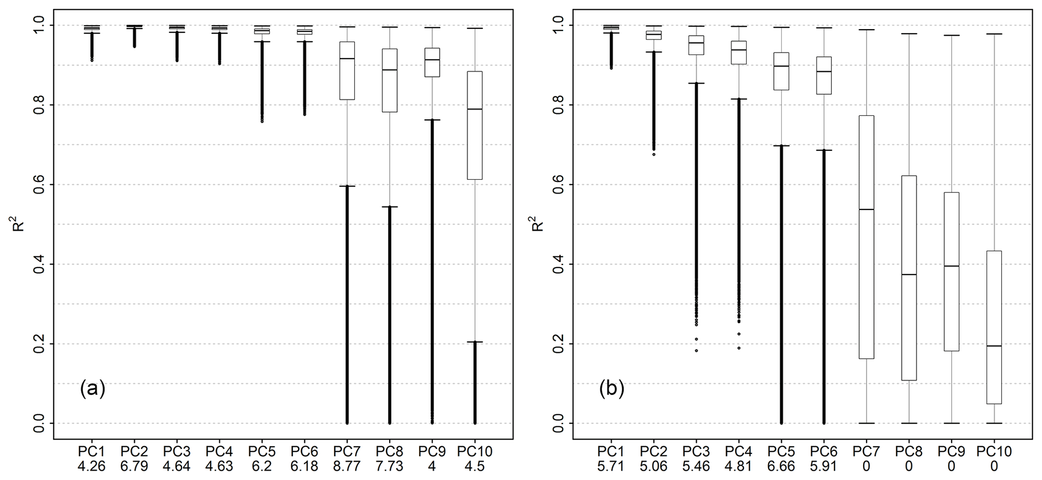
Figure 3 Comparison of the PCA results of the stability analysis. (a) Correlation of loadings based on the random subsampling of the measurement dates to assess the stability of spatial patterns. (b) Correlation of scores based on the random selection of observation wells, i.e. complete series, to assess the stability of temporal patterns. The boxes indicate the quartiles; the whiskers all dates indicate which are within the range of the first quartile of −1.5 times the interquartile range or the third quartile of +1.5 times the interquartile range, respectively. Percentage of values outside the whiskers of a boxplot is given in the labelling of the x axis for each PC.

The comparison of the temporal patterns of the PCAs which were performed with the subdatasets based on the random selections of observation wells, i.e. complete series, is summarized in Fig. 3b. Generally, with an increasing rank of the PCs the median correlation between the scores of the PCs of the different PCAs was decreasing, and the variability of correlation between the scores was increasing (Fig. 3b). Only the first four PCs exhibited notably stable temporal patterns with a median correlation of R²>0.9.

Figure 4 Time series of scores of the stable PCs 1 to 4.

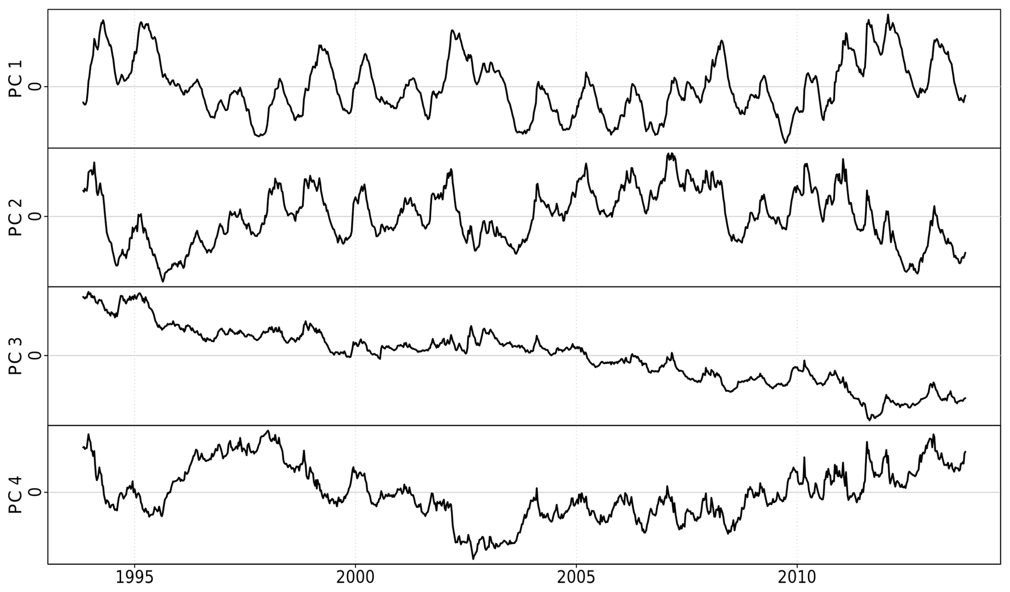
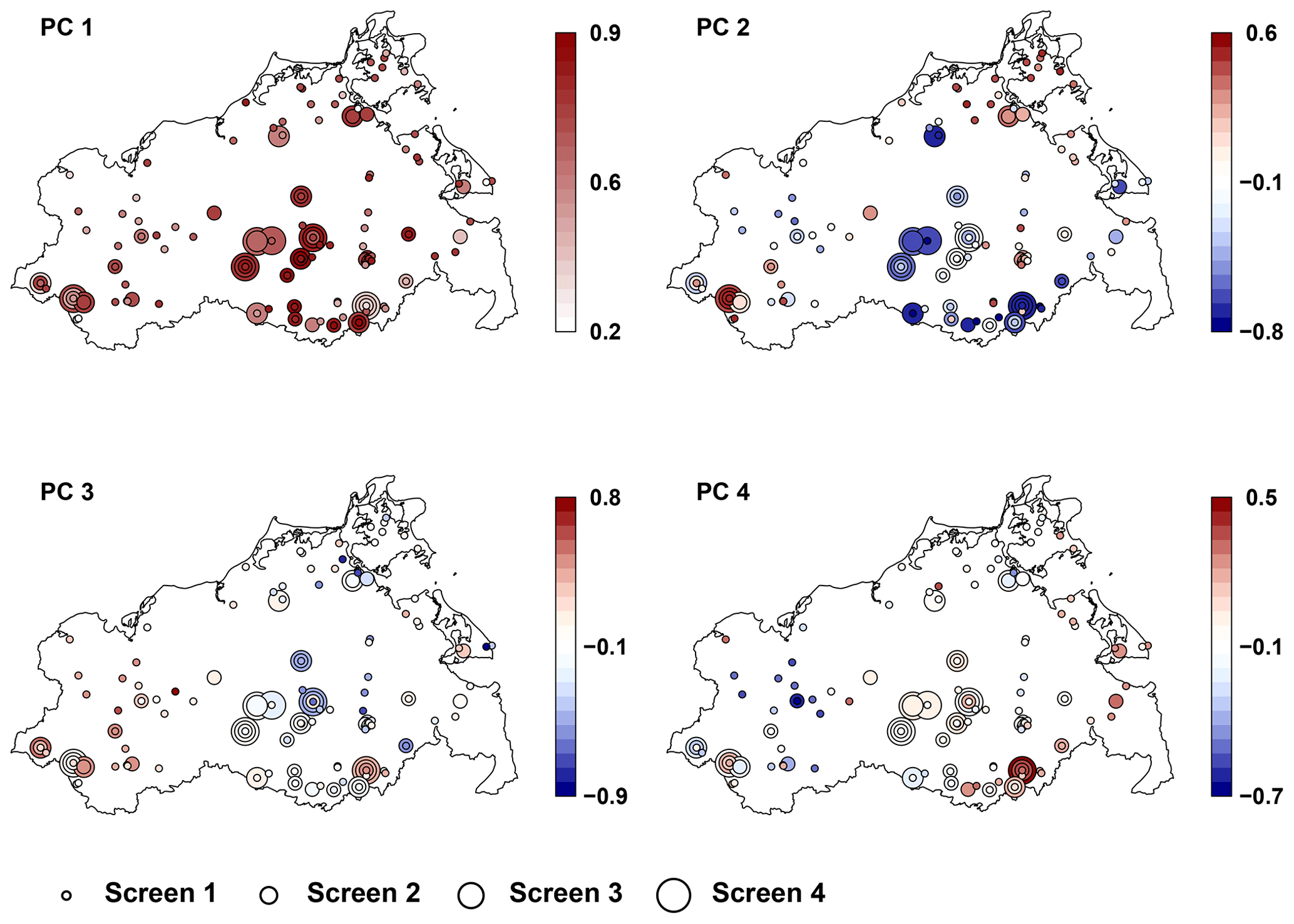
Figure 5 Spatial patterns of loadings of the stable PCs 1 to 4.

Accordingly, the first four PCs were considered stable on the scale of the network, accounting for 80.8 % of the observed variance in the groundwater head series. The variance was assigned as follows: 48.3 % for PC 1, 17.2 % for PC 2, 9.5 % for PC 3, and 5.8 % for PC 4. The assigned temporal and spatial patterns of the complete dataset with all 141 series are shown in Figs. 4 and 5. In the following the analysis is restricted to these four stable PCs.

4.2 Well-specific reference hydrograph and residuals

At each well, the residuals of the reference hydrograph were checked for peculiarities. We present here two examples. At well Deven (Fig. 6) the observed hydrograph was in general very well represented by the well-specific reference hydrograph (R²=0.84). The mean depth to groundwater was 9.52 m. A single period stuck out in the plot of the residuals. At the end of October 1998 the residuals showed a sudden shift of approximately 17 cm towards a higher water level, followed by a similar sudden shift “back to the old level” in December 1999. Those shifts were not clearly identifiable in the observed time series itself nor in the reference hydrograph.

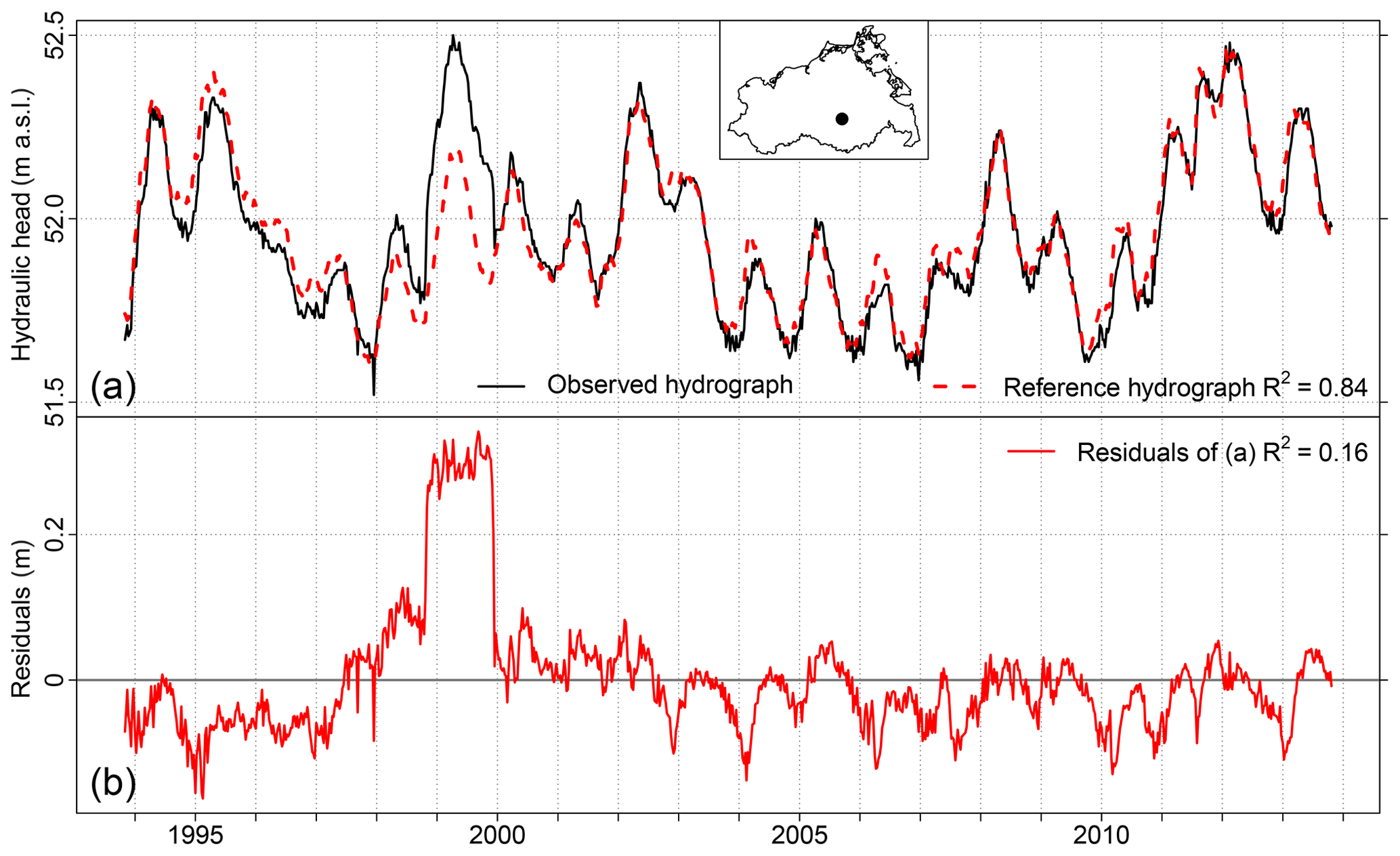
Figure 6 (a) Time series of the hydraulic head and the reference hydrograph of well Deven. (b) Time series of residuals. Location of the well is marked as a black dot in the inset map. Height of the well head at well Deven is 61.48 m a.s.l. Correlation of the observed series with the reference hydrograph and with the residuals is given as R².

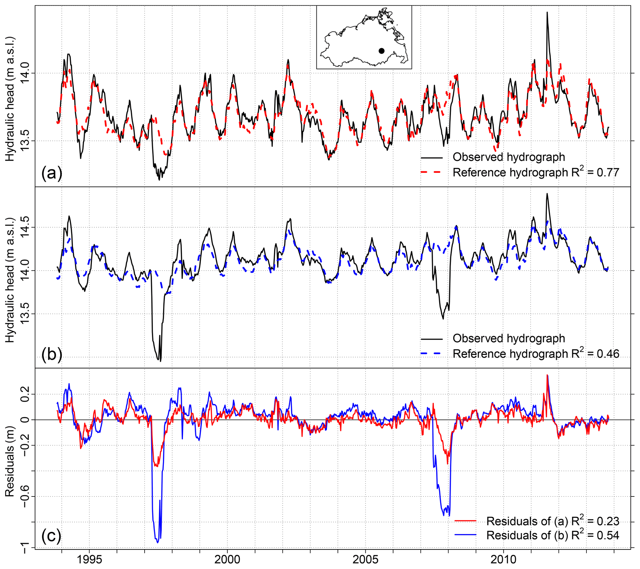
Figure 7 Time series of hydraulic head and the reference hydrograph of (a) well Neubrandenburg UP and (b) well NB-Hotel Vier Tore. (c) Time series of residuals. Location of the wells is marked as a black dot in the inset map. Height of the well head at well Neubrandenburg UP is 18.3 m a.s.l.; at well NB-Hotel Vier Tore it is 17.86 m a.s.l. Correlation of the observed series with the reference hydrograph and with the residuals is given as R².

Observation well Neubrandenburg UP exhibited in general a relatively good fit of observed series and the reference hydrograph (R²=0.77) with the exception of two anomalous periods in 1997–1998 and 2007–2008, a series of minor deviations before 1997, and another relatively strong deviation in 2011 (Fig. 7a and c). The mean depth to groundwater was 4.61 m. For comparison we considered the nearby observation well NB-Hotel Vier Tore approximately 600 m further south which was formerly excluded from the PCA due to known anthropogenic influence (Sect. 2.2). The mean distance of the well head to the groundwater level was 3.74 m. Here we calculated the reference hydrograph in the same manner as multiple linear regression of the observed hydrograph with PCs 1–4. Again the observed series exhibited in general a relatively good fit with the reference hydrograph (Fig. 7b and c). However, compared to observation well Neubrandenburg UP the two periods of strong deviation in 1997–1998 and 2007–2008 were more pronounced in the residuals and, in contrast to observation well Neubrandenburg UP, clearly visible in the observed series as well. This was reflected in a substantially weaker correlation between the observed series and the reference hydrograph (R²=0.46).

5 Discussion

5.1 Stability of PCs

To select only those PCs which are representative for the monitored region in the analysed period, a series of PCAs were performed based on randomly selected subsets of the complete dataset to identify the stable PCs. The stable PCs are those of which the assigned spatial patterns (loadings) and temporal patterns (scores) were rather insensitive to the selection of analysed observation wells and measurement dates. Only the stable PCs were considered for the further analysis.

Earlier studies which used PCA to summarize hydrological variability in a region analysed the stability of their results in a similar way (Smirnov, 1973; Lins, 1985a). Those attempts were limited to the comparison of the PCAs of a few different configurations of the dataset. The correlation analysis in this study extended the assessment of stability of the PCs towards random selections of the analysed data in both the spatial and the temporal domain and a substantially larger number of different configurations of the analysed dataset.

The comparison of the results of the 10 000 PCA variants revealed that the stability of individual PCs decreased in general with a decreasing rank of the PCs (Fig. 3). Clear differences between the stability of temporal and spatial patterns of the PCs were observed. PCA results were more sensitive to changes in the selection of the observation wells considered (Fig. 3b) than to changes in the selection of measurement dates (Fig. 3a). This likely reflects the stronger mean correlation between subsequent observations at the sites (temporal autocorrelation) compared to the mean correlation of the series of the closest adjacent sites (correlation in the spatial domain) (Sect. 2.2). The first four PCs were found to be stable (Fig. 3). This gave some confidence that their spatial and temporal patterns were indeed characteristic for the monitored region in the analysed period and not restricted to the specific selection of observation wells or measurement dates. Compared to the established Kaiser criterion (Sect. 3.2), the number of PCs considered was reduced from 10 to 4.

5.2 Well-specific reference hydrographs and residuals

The well-specific peculiarities in the time series of the residuals of the reference hydrographs might be of different origins. First of all they might be caused merely by technical problems. For example we interpreted the single period in 1999 which sticks out in the plot of the residuals of observation well Deven as a stepwise shift of the logger (Fig. 6b). This shift was in phase with the seasonal pattern of the observed series and was therefore not obvious from the visual inspection of the observed series alone, while it was clearly visible in the residuals.

An example of well-specific peculiarities in the residuals due to local anthropogenic influence is given in Fig. 7. Observation well NB-Hotel Vier Tore was excluded from the PCA because its hydrograph was known to be influenced by the lowering of the groundwater level during the construction of an underground car park approximately 100 m away in 1997–1998 and the construction of another underground car park approximately 200 m away in 2007–2008. While this influence was clearly visible in the observed series at that observation well (Fig. 7b), it was not obvious in the observed series at observation well Neubrandenburg UP, especially not the second deviation in 2007–2008 (Fig. 7a). This is most probably because Neubrandenburg UP was further away from both construction sites, namely approximately 400 m from each. However, in the residuals both periods became clearly visible for both observation wells although to different degrees at the two wells (Fig. 7c).

Such clear assignment of anthropogenic influence to a local deviation from the regional behaviour is only possible if the scale of the respective effect is rather local in comparison to the scale of the monitoring network as a whole and the scale of the spatiotemporal resolution of the network in particular. The latter enables a distinct localization of the influence. An anthropogenic effect which induces similar groundwater head dynamics at a substantial amount of the series of the dataset would be incorporated into the leadings PCs (Wriedt, 2017) and thus would affect the reference hydrographs. However, such an effect is hardly likely. Moreover, the approach presented does not differentiate anthropogenic from “natural” effects per se. Rather, it decomposes the time series into regional patterns which can be assigned to many or all time series of the dataset and local patterns which are restricted to a few or single sites. Another restriction is that PCA based on z-scaled series considers only temporal patterns of the groundwater head, but it ignores the absolute values. Thus, it does not allow any inferences as to whether the observed groundwater head on average is higher or lower than it would be under natural conditions. Then again, the z scaling of the series makes the analysis robust against systematic differences or discontinuities in the spatial distribution of mean groundwater recharge.

The spatial clustering of observation wells indicated a spatial bias of the monitoring (Fig. 1). It reflected the focus of the monitoring on anthropogenic water use, for example close to settlements, towns, etc., which is a prerequisite for sustainable water management. Because all the series were equally weighted by z scaling (Sect. 3.1), the derived PCs, and consequently the determined normal behaviour, was distorted towards areas with a higher density of observation wells (Karl et al., 1982) as well as towards smaller mean depths to groundwater (Fig. 2). This should be considered for any interpretation of the reference hydrographs as well as of their local deviations. However, in this study, the stable PCs used for the calculation of the reference hydrographs turned out to be rather robust with respect to the selection of observation wells (Sect. 4.1), suggesting that the results were not primarily determined by the local clustering of the observation wells.

In general, the reference hydrograph is a relatively good-natured and robust PCA application for mainly two reasons. First, the selection of the PCs considered is transparent and reproducible. The approach prevents the consideration of PCs which exhibit pronounced instability of the associated spatial and temporal patterns, for example PCs with “degenerate eigenvalues”, that is eigenvalues which are indistinguishable within their range of uncertainties (Hannachi et al., 2007). Second, the single PCs are not used, but the combination of the stable PCs are. Thus, it is not necessary to interpret single PCs as drivers of groundwater head variability or distinct processes. Consequently, describing the regional behaviour with the reference hydrograph is also applicable in cases in which the interpretation of single PCs is severely hampered, for example if the associated spatial patterns of the PCs mainly reflect the shape of the analysed domain (domain shape dependence) (Buell, 1975, 1979; Richman, 1986, 1993).

Some PCA applications involve rotation of the considered PCs to achieve more simple structures, i.e. more localized spatial patterns, which might support the interpretation of single PCs (Lins, 1985b; Richman, 1986; Jolliffe, 1987, 2002; Hannachi et al., 2007). It is possible to combine such applications with the reference hydrograph application. For the suggested screening application, rotating the PCs does not change the results as long as the rotation is performed with all stable PCs or only with a subset of the stable PCs. In this case the reference hydrographs and their residuals are the same whether they are calculated from the rotated or the unrotated PCs. Concerning the reference hydrographs, the decisive question is which PCs are included in the calculation.

The approach presented uses the spatiotemporal variability in a large set of groundwater head series to determine individual reference hydrographs for each observation well. Thus, it requires neither the identification of clusters of similar wells or single reference wells nor assumptions about the catchments of the wells, hydraulic connection between the wells, etc. This is in contrast to approaches which select some of the monitored wells as reference observation wells being representative for the whole monitoring network or for subgroups or subregions only. For example other PCA applications used the clustering of observation wells in the scatterplot of loadings of PC 1 versus PC 2 to identify “index” wells for each cluster (Winter al., 2000) or applied PCA directly to subgroups of a monitoring network, which were determined based on an estimation of the physical relatedness of the observation wells earlier, to firstly identify the “principal wells” of the subgroups and subsequently identify the most representative wells for the whole network by ranking all wells according to their number of occurrences as a principal well (Gangopadhyay et al., 2001).

However, despite the different approaches of how to determine the most representative observation wells, it has to be considered that observation wells which are of little representative value for the whole monitoring network might be of high informative value, for example with respect to anthropogenic influence that is specific to single observation wells. In contrast to the selection of single wells which are considered especially representative or atypical for the network, the suggested approach in this study enables a quick ordering of all wells in a network according to their representativeness and yields an estimation of the local well-specific behaviour for each well.

5.3 Other applications

In addition to the presented applications in this study, other applications of the reference hydrographs and residuals are possible. One option is to use the series of the stable PCs (scores) as predictor variables in a linear regression to fill gaps in hydraulic-head series which were not analysed with the PCA but which exhibit some overlap with the monitoring period covered by the PCA. For example the reference hydrograph at observation well NB-Hotel Vier Tore (Fig. 7b) was calculated although the groundwater head series was not part of the PCA. In this study it was merely used for the identification of the influence of the construction works, but it could be used to replace the periods which were influenced by the construction works with an estimation of unaffected groundwater head dynamics as well (Fig. 7b). In the spatial domain, calculating the Pearson correlation of excluded series with the stable PCs for limited overlapping time periods can be used to extend the spatial coverage of the maps of the loadings. For both applications, the random subsampling analysis can be used to estimate how many missing values in the series might be tolerable. For this dataset we would be confident to consider series with up to 30 % of missing values during the 20-year period. The maximum time gap in this study was 88 d (Sect. 2.2), and most of the time gaps were substantially smaller (Fig. S2). Thus, the results are most likely less stable for a few long gaps compared to numerous but short gaps.

Another application is to identify distinct reference observation wells by selecting those observation wells at which the correlation between the reference hydrograph and the observed series is above a certain threshold, for example R²>0.9. Those would be considered the most representative observation wells for the whole monitoring network. In case the period covered by the series of the reference observation wells exceeds the period covered by the PCA, they can be used as predictor variables in a linear regression to extrapolate the series of the stable PC scores.

The methods to extend the spatial and temporal coverage of the PCs should be handled with care. However, because only the stable PCs were used, there should be no major bias, as long as the extension is performed only for some years or a small number of additional series. If new data are available that cover a larger area or a longer period, it is in general preferable to perform a new PCA with all available data to account for systematic changes in the temporal dynamics of the analysed groundwater system and systematic changes in the monitoring network geometry and spatial distribution of the observation wells.

The detection of changes in characteristic temporal patterns (scores) and their occurrence in the monitoring network (maps of the loadings) between different observation periods is another application of the reference hydrographs and their residuals. It has to be noted that a direct comparison of the temporal patterns of two periods can only be performed for temporally overlapping periods. For non-overlapping periods, a comparison is restricted to general time series characteristics, for example the timing or amplitude of a seasonal pattern.

6 Conclusions

The application of the reference hydrographs and their residuals proved to be a straightforward way to check the data for measurement errors and to identify candidates for local anthropogenic influence. Both applications are actually an interpretation of the temporal dynamics of local anomalies in the observed groundwater head series. In contrast to other approaches the identification of those local anomalies is based on the correlation among the observed groundwater head series only and not based on physical models or empirical relationships with any predictor of groundwater head dynamics. The assignment of local anomalies to the residuals is not restricted to specific types of temporal patterns. The residuals merely comprise what cannot be ascribed to the reference hydrographs by means of the stable PCs. This can be short-term structures like sudden shifts or distinct periods of deviation as well as long-term structures like drifts, trends, or cyclic patterns. The presented approach also does not require an interpretation of single PCs as distinct physical processes or functional relationships. This limitation with respect to the direct physical interpretation of the results brings with it the benefit that the only information required is series of (groundwater) hydraulic-head readings all measured at the same instants of time. Other suggested applications for the stable PCs are for example data-driven gap filling in the observed series, spatial and temporal extrapolation of the reference hydrographs, or the identification of distinct reference observation wells. The approach to determine the stable PCs is transparent and reproducible.

The computational demand is very low. Time series of the well-specific deviations from normal behaviour (residuals) are easily derived and enable a fast screening for well-specific peculiarities. In monitoring practice, ranking all wells in the network according to their normality can be used to distribute resources, in particular to support the decision which observation wells, i.e. which series, should be investigated in more detail. Especially for larger datasets it can be helpful to apply time series tools like filters to identify for example step changes or trends in the analysis of the residuals. Those tools can be easily incorporated into the workflow once the residuals are derived. However, based on our experience, we advocate that visual inspection should be included in the quality check workflow as well. Furthermore the residuals can be used to categorize the deviations from the normal behaviour. Thus, we recommend the approach presented as a fast screening tool for the assessment of comprehensive groundwater monitoring networks.