the Creative Commons Attribution 4.0 License.
the Creative Commons Attribution 4.0 License.
 | 13 Oct 2020
Assessing global water mass transfers from continents to oceans over the period 1948–2016
Denise Cáceres
Ben Marzeion
Jan Hendrik Malles
Benjamin Daniel Gutknecht
Hannes Müller Schmied
Petra Döll
Ocean mass and thus sea level is significantly affected by water storage on the continents. However, assessing the net contribution of continental water storage change to ocean mass change remains a challenge. We present an integrated version of the WaterGAP global hydrological model that is able to consistently simulate total water storage anomalies (TWSAs) over the global continental area (except Greenland and Antarctica) by integrating the output from the global glacier model of Marzeion et al. (2012) as an input to WaterGAP. Monthly time series of global mean TWSAs obtained with an ensemble of four variants of the integrated model, corresponding to different precipitation input and irrigation water use assumptions, were validated against an ensemble of four TWSA solutions based on the Gravity Recovery and Climate Experiment (GRACE) satellite gravimetry from January 2003 to August 2016. With a mean Nash–Sutcliffe efficiency (NSE) of 0.87, simulated TWSAs fit well to observations. By decomposing the original TWSA signal into its seasonal, linear trend and interannual components, we found that seasonal and interannual variability are almost exclusively caused by the glacier-free land water storage anomalies (LWSAs). Seasonal amplitude and phase are very well reproduced (NSE=0.88). The linear trend is overestimated by 30 %–50 % (NSE=0.65), and interannual variability is captured to a certain extent (NSE=0.57) by the integrated model. During the period 1948–2016, we find that continents lost 34–41 mm of sea level equivalent (SLE) to the oceans, with global glacier mass loss accounting for 81 % of the cumulated mass loss and LWSAs accounting for the remaining 19 %. Over 1948–2016, the mass gain on land from the impoundment of water in artificial reservoirs, equivalent to 8 mm SLE, was offset by the mass loss from water abstractions, amounting to 15–21 mm SLE and reflecting a cumulated groundwater depletion of 13–19 mm SLE. Climate-driven LWSAs are highly sensitive to precipitation input and correlate with El Niño Southern Oscillation multi-year modulations. Significant uncertainty remains in the trends of modelled LWSAs, which are highly sensitive to the simulation of irrigation water use and artificial reservoirs.
- Article
(3049 KB) - Full-text XML
-
Supplement
(1096 KB) - BibTeX
- EndNote


Global mean sea level rise has been widely used as an indicator of the impact of climate change on the Earth system. In recent decades, it has mainly been caused by anthropogenic climate change (Slangen et al., 2016), but it has also been affected by direct human interventions such as the impoundment of water in artificial reservoirs and water abstractions on the continents (Chao et al., 2008; Church et al., 2013; Oppenheimer et al., 2019). Since the beginning of the satellite altimetry era, several missions have produced continuous measurements of sea level height to monitor its evolution. Primarily, sea level change can be decomposed into a steric component (i.e. thermal expansion and salinity change) and a mass component (i.e. ocean mass change). Since the beginning of the 21st century, the Gravity Recovery and Climate Experiment (GRACE) satellite mission has made the monitoring of spatially and temporally distributed ocean mass change possible. Moreover, according to the principle of water mass conservation in the Earth system, the latter can be estimated as being the sum of temporal changes in mass of (1) Greenland and Antarctica ice sheets, (2) glaciers, (3) water stored on the continents (excluding glaciers) and (4) atmospheric water vapour. If the water mass in these four compartments decreases, ocean mass increases. A number of studies (Church et al., 2013; Chambers et al., 2017; Dieng et al., 2017; WCRP, 2018) have shown that it is possible to reconstruct the time series of global mean sea level change by summing up changes in the individual components within the uncertainties of the observational estimates. However, substantial uncertainty remains for individual components; this is the case in the net contribution of continental water storage change to ocean mass change for which an accurate quantification continues to be a challenge (WCRP, 2018). One way of assessing this contribution is through the usage of GRACE observations over the continents. However, GRACE observations cannot distinguish between mass changes in glaciers and in water stored elsewhere on the continents, such as soils, surface water bodies or groundwater, nor can reasons for mass changes be explored. In addition, GRACE records only start in 2002 and contain some temporal gaps.
In ocean mass budget studies, continental water storage change is usually decomposed into changes in mass of glaciers and of water stored in glacier-free land. To determine temporal mass changes, it is not necessary to compute the time series of total mass but only the time series of mass anomaly, i.e. mass variations as compared to a mean value over a specific time period. Hereafter, we refer to glacier mass as the land glacier water storage anomaly (LGWSA), which does not include ice sheet peripheral glaciers, and to water mass on glacier-free land as the land water storage anomaly (LWSA). LWSA is the sum of water stored in rivers, lakes, wetlands, artificial reservoirs, snow pack, canopy and soil and as groundwater, excluding glaciers (Church et al., 2013; Scanlon et al., 2018). It can also be disaggregated into a climate-driven (LWSAclim) and a human-driven component (LWSAhum). The sum of LGWSA and LWSA equals the total continental water storage anomaly (TWSA).
The distinction between LGWSA and LWSA in ocean mass budget assessments stems partly from the fact that global glacier mass loss is known to be the main driver of water transfers from continents to oceans during the 20th century and in the early 21st century (Zemp et al., 2019) and the rest of this century (Hirabayashi et al., 2013; Slangen et al., 2017; Hock et al., 2019). There are currently several global glacier models capable of simulating LGWSA at the global scale (Hirabayashi et al., 2013; Marzeion et al., 2012; Huss and Hock, 2015). LWSA can be derived from global hydrological and land surface models (GHMs). For instance, Munier et al. (2012) estimated LWSAs for the period 1993–2009 over the global continental area by averaging the output of three GHMs. On the other hand, various other approaches have been employed to estimate LWSAs. Dieng et al. (2015) used a global ocean mass budget approach over 2003–2013; they compared GRACE-based ocean mass change to the sum of mass components derived from independent products, except for LWSA, which was the unknown quantity to be estimated. In other studies, this component was extracted from GRACE-derived TWSA (Reager et al., 2016; Rietbroek et al., 2016). Wada et al. (2017) assessed components of LWSAs based on (1) modelling groundwater depletion with PCR-GLOBWB, (2) estimating impoundment behind dams by adding storage capacities of reservoirs (updated from Chao et al., 2008), (3) assuming the LWSAclim estimate of Reager et al. (2016) and (4) very roughly estimating storage losses in endorheic lakes (Caspian Sea and Aral Sea), wetlands and due to deforestation based on literature. Because LWSA involves multiple water storage compartments and is not only driven by climate variability and change (LWSAclim) but also human activities (LWSAhum), its assessment remains highly uncertain.
To fill this key knowledge gap related to the TWSA and, more particularly, the LWSA component of ocean mass change, we did a long-term (1948–2016) assessment of TWSAs over the global continental area (except Antarctica and Greenland). Our assessment provides not only the total contribution of continents to oceans but also quantifies the separate contributions of the individual components of TWSAs. In the first instance, we disaggregated TWSAs into the contributions of LGWSA, LWSAclim and LWSAhum (the sum of the latter two components is equal to LWSA). We further disaggregated LWSAhum by quantifying separately the effect of water impoundment in reservoirs (LWSAres) and the effect of water abstraction (LWSAabs) and related LWSAclim to global annual precipitation and to the El Niño–Southern Oscillation (ENSO). TWSA estimates were obtained by combining two state-of-the-art global models, namely the global glacier model (GGM) of Marzeion et al. (2012) and the GHM WaterGAP (Döll et al., 2003; Müller Schmied et al., 2014, 2016). In its standard version, WaterGAP simulates storage changes in all compartments except glaciers. Areas that, in reality, are covered by glaciers (hereafter glacierized areas) are treated as normal (i.e. non-glacierized) areas. To account for glacierized areas and the effect of glacier mass variability on water flow dynamics on the continents, we integrated a 0.5∘ gridded annual time series of glacier area and a monthly time series of LGWSA simulated by GGM as an input to WaterGAP. This resulted in a non-standard version of WaterGAP, which includes the impact of glaciers on water storages and flows, hereafter referred to as integrated WaterGAP. The model was run with two different precipitation forcings and two different assumptions regarding irrigation water use, resulting in an ensemble of four solutions. We regarded the spread of these four time series around the ensemble mean as being an informal indication of uncertainty. We validated the ensemble by comparing it to an ensemble of four GRACE spherical harmonic (SH) solutions. Through this comprehensive assessment, we aimed to address the following questions:
-
How did changes in total water storage on the continents of the Earth (except Greenland and Antarctica) contribute to ocean mass changes (and thus sea level change) during the period 1948–2016? (See Sect. 3.2.1.)
-
Which continental storages underwent the most significant mass changes during this period? (See Sects. 3.2.2 and 3.2.5.)
-
How have artificial reservoirs and human water abstractions affected water storage on the continents? (See Sect. 3.2.3.)
-
What were the main climatic drivers of glacier-free land water storage changes? (See Sect. 3.2.4.)
-
To what extent can we rely on our modelling approach to quantify global-scale water storage changes on the continents? (See Sects. 3.1 and 4.2.)
Our assessment is innovative regarding (1) the modelling approach, which combines the strengths of two well-established global models, (2) the validation approach, which consisted of comparing TWSAs over the global continental area from modelling and GRACE in terms of seasonality, linear trend and interannual variability, and (3) the disaggregation of TWSAs into individual mass components and drivers.
In the following section, we describe the models, data sets and methods used in this study. In Sect. 3, we present the results of our model validation and of our assessment of global TWSAs over 1948–2016. The results are discussed in Sect. 4. Finally, we present our conclusions in Sect. 5.
2.1 Models
2.1.1 Global hydrological model
We used the latest version of the GHM WaterGAP, namely WaterGAP2.2d. It simulates human water use and daily water flows and water storages (or anomalies) on a 0.5∘ by 0.5∘ grid (55 km by 55 km at the Equator and ∼3000 km2 grid cell), covering the global continental area – except for Antarctica (see Fig. 1 in Döll et al., 2014). Streamflow is laterally routed through the stream network derived from the global drainage direction map DDM30 (Döll and Lehner, 2002) until it reaches the ocean or an inland sink. Calibration is performed against observations of mean annual streamflow at 1319 gauging stations (Müller Schmied et al., 2014). Daily climatological input data sets of precipitation, near-surface air temperature and long- and short-wave downwards surface radiation are required as input. We used a homogenized climate forcing resulting from the combination of WATCH Forcing Data (WFD) based on ERA-40 reanalysis (Weedon et al., 2011) for the period 1948–1978 and WFD methodology applied to ERA-Interim (EI) reanalysis (hereafter referred to as WATCH Forcing Data ERA-Interim – WFDEI; Weedon et al., 2014) for the period 1979–2016 (Müller Schmied et al., 2016). Monthly sums of precipitation are bias corrected by monthly precipitation data sets derived from rain gauge observations of either the Global Precipitation Climatology Centre (GPCC) version 5 and/or version 6 (Schneider et al., 2015) or the Climate Research Unit (CRU) TS3.10 and/or TS3.21 (Harris et al., 2014). Note that the GPCC and CRU products used to scale monthly precipitation sums within WFDEI use the available number of stations for each month. The variability in the number of observations over time makes the resulting precipitation data sets less suitable for trend analysis. However, as we are not aware of an available long-term global precipitation data set with high station density that could be used instead, note that the benefits of including those adjustments into reanalysis products due to, for example, the incorporation of snow undercatch corrections result in more plausible hydrological studies (Kauffeldt et al., 2013; Müller Schmied et al., 2016). We forced WaterGAP with both WFDEI, with monthly precipitation sums based on GPCC (hereafter WFDEI–GPCC), and on CRU (hereafter WFDEI–CRU) to account for part of the uncertainty due to precipitation input data.

Figure 1Schematic of integration of glacier data from the global glacier model (GGM) into WaterGAP at grid cell scale. Glacier data sets are represented by orange boxes. Blue boxes represent water storage compartments in WaterGAP (for definitions of the abbreviations, refer to Eq. 2). Full arrows represent water flows, and dotted arrows indicate that the sum of changes in individual storages equals total water storage change. See text for details and abbreviations.
WaterGAP simulates the impact of water impoundment in reservoirs and of human water use on water flows and storages. LWSAhum is calculated following Eq. (1):
where LWSAres is the anomaly due to impoundment of water in reservoirs, and LWSAabs is the anomaly due to water abstraction. Reservoir data used by the model comes from a preliminary version of the Global Reservoir and Dam (GRanD) database, which includes 6862 reservoirs with a total storage capacity of 6197 km3 (Lehner et al., 2011). The simulation of reservoir operation is based on a slightly modified version of the algorithm of Hanasaki et al. (2006), which distinguishes between irrigation and non-irrigation reservoirs (Döll et al., 2009). The model distinguishes between artificial reservoirs and regulated lakes (i.e. natural lakes whose outflows are regulated by a dam). Reservoirs (i.e. artificial reservoirs plus regulated lakes) are classified as either local, meaning that they are fed only by runoff produced within the cell, or global, meaning that they are also fed by streamflow from the upstream cell. They are assumed to be global if their maximum storage capacity is at least 0.5 km3 or their surface area is at least 100 km2. Since global reservoirs may spread over more than one grid cell, their water balance is computed in the outflow cell. Local lakes and local reservoirs within one cell are lumped into one local lake. Lumping multiple local reservoirs within one cell into one local reservoir inevitably erases the specific characteristics of each reservoir; the resulting lumped local reservoir is then not expected to be better simulated by the reservoir algorithm than by the lake one (Döll et al., 2009). In total, 1082 global artificial reservoirs and 85 global regulated lakes, which together represent a total storage capacity of 5764 km3 (∼16 mm SLE), are simulated by WaterGAP using the reservoir algorithm. The reservoir-filling phase upon construction is simulated based on the first operational year and the storage capacity. The monthly release flow of irrigation reservoirs varies according to the downstream consumptive water use (i.e. part of water abstractions that evapotranspires during use). For non-irrigation reservoirs, it is assumed that the release flow remains unchanged throughout the year if the storage capacity to mean total annual outflow ratio is larger than 0.5, while it otherwise depends, also in case of irrigation reservoirs, on daily inflows into the reservoir.
Concerning human water use, in a first instance, time series of water abstraction and consumptive water use are generated for five water use sectors (irrigation, livestock farming, domestic use, manufacturing industries and cooling of thermal power plants) by separate global water use models. The calculation of irrigation water use takes into account climate variability and yearly country estimates of the irrigated area (Döll et al., 2012). The outputs of the water use models are then translated into net abstraction (i.e. total abstraction minus return flow) by the sub-model Groundwater–Surface Water Use (GWSWUSE), which distinguishes the source of abstracted water (surface water or groundwater). The net abstraction time series are then subtracted from the surface water and groundwater storage compartments of WaterGAP, respectively (Müller Schmied et al., 2014; Döll et al., 2014).
2.1.2 Global glacier model
We used the global glacier model (GGM) of Marzeion et al. (2012). The model computes mass changes in individual glaciers for the whole globe. It combines a glacier surface mass balance model, following an empirically based temperature index approach, with a model that accounts for the response of glacier geometry (in the model defined by area, length and elevation range) to changes in glacier mass. The dynamic simulation of this response follows an area–volume–time scaling approach, based on the equation of Bahr et al. (1997), enabling the model to account for various types of feedback between glacier geometry and mass balance. The model is calibrated by fitting simulated glacier surface mass balance to observations from the collections of the World Glacier Monitoring Service (2016). The error in modelled annual glacier mass change is determined using a cross-validation routine applied to glaciers with observed mass balances.
GGM is forced by global time series of near-surface air temperature and precipitation fluxes. For this study, we used the mean of an ensemble of seven global gridded atmospheric data sets (New et al., 2002; Saha et al., 2014; Compo et al., 2011; Dee et al., 2011; Kobayashi et al., 2015; Poli et al., 2016; Gelaro et al., 2017), as choosing the ensemble mean over any of the individual data sets allows the reduction of the uncertainty due to input climate forcing data. As initial conditions, it also requires information on glacier area and minimum and maximum elevation, which are taken from the Randolph Glacier Inventory (RGI) version 6.0 (updated from Pfeffer et al., 2014). GGM includes both local (i.e. glacier-specific) and global parameters. Local parameters are calibrated and cross-validated following the procedure described in Marzeion et al. (2012). Global parameters are optimized following a multi-objective optimization routine, maximizing the temporal correlation of model results and observations and minimizing the model bias as well as the difference in the variance of modelled and observed mass balances.
2.2 Data
By combining WaterGAP, capable of simulating LWSA (Sect. 2.2.1), and GGM, capable of simulating LGWSA (Sect. 2.2.2), through a data integration approach (Sect. 2.3.1), we obtained global time series of TWSAs and individual components at monthly scale over 1948–2016. We evaluated the LGWSA data set against annual and seasonal time series of glacier mass change from in situ observations (Sect. 2.2.3). The modelled global TWSA time series were evaluated using global GRACE-derived TWSA time series at a monthly scale, covering the period from January 2003 to August 2016, with some months with missing data in between (Sect. 2.2.4).
2.2.1 Modelled LWSA
WaterGAP simulates the transport of water on continents as flows among all continental water storage compartments, except for glaciers (see Fig. 1 in Döll et al., 2014). Glacierized areas are treated as non-glacierized areas. LWSA is calculated following Eq. (2):
where WSA is the water storage anomaly in snow (Sn), canopy (Cn), soil moisture (SM), groundwater (G), lake (La), reservoir (Re), wetland (We) and river (Ri) storages.
2.2.2 Modelled LGWSA
GGM computes glacier mass change at the scale of individual glaciers; however, for this study the data were provided on a rectangular 0.5∘ by 0.5∘ grid covering the entire globe (excluding ice sheet peripheral glaciers). Gridded annual time series of glacier area computed with GGM and monthly time series of total (liquid plus solid) precipitation on glacier area from the atmospheric forcing were also used in this study. Glacier area data were required to adapt the land area fraction within WaterGAP cells. In addition, precipitation on glacier area was required to calculate glacier runoff (Sect. 2.3.1). Note that, to produce the gridded GGM data sets, each glacier was assigned to the grid cell that contains its centre point (as given in the RGI version 6.0) even if, in reality, the glacier stretches across several grid cells. Furthermore, we applied a number of preprocessing steps to the GGM gridded data in order to make it suitable as input data for WaterGAP (described in Sect. S1.1 of the Supplement).
2.2.3 Glacier mass change from in situ observations
Time series of annual and seasonal glacier surface mass balance at the scale of individual glaciers derived from in situ observations from the reference glaciers sample of the World Glacier Monitoring Service (2017) were used to evaluate the performance of GGM. This constitutes a reliable and well-documented sample of globally distributed long-term observation series. With the term seasonal, we refer to the winter and summer seasons within a glacier mass balance year. During the winter (accumulation) season, the glacier tends to gain mass, while during the summer (melting) season, it tends to lose mass. A glacier was selected from the sample if (1) its observations corresponded to the entire glacier and not solely to sections of it, (2) it had a minimum of 5 years of observations for both summer and winter and (3) it was among the glaciers simulated by GGM. In total, 31 glaciers were selected (see Table S1 in the Supplement).
2.2.4 GRACE-derived TWSA
Global time series of mass change over continents were derived from ITSG-Grace2018 (Mayer-Gürr et al., 2018) and GRACE Release 06 (Center for Space Research – CSR; German Research Centre for Geosciences – GFZ; and Jet Propulsion Laboratory – JPL) quasi-monthly Level-2 gravity field solutions by means of global SH coefficients. We further processed the SH solutions in order to derive global grids of surface mass change. Monthly resolved solutions expanded up to degree and order 60 were chosen for the lower noise level compared to higher resolved solutions. We substituted Degree-1 (geocentre motion) coefficients following the approaches of Swenson et al. (2008) and Bergmann-Wolf et al. (2014) and C2,0 (Earth's oblateness) coefficients after Cheng et al. (2013), respectively. Gravity changes related to glacial isostatic adjustment (GIA) were accounted for using GIA modelling results from Caron et al. (2018). Furthermore, we excluded areas with considerable mass redistribution related to the 2004 and 2005 earthquakes in Sumatra–Andaman and Nias–Simeulue, Indonesia, and the 2011 Tōhoku, Japan, earthquake from the integration. As we preferred unconstrained SH solutions over a priori regularized mascon products, we corrected for the coastal leakage effect from continent to ocean by expanding the initial land–water mask by placing a 300 km buffer onto the ocean. The gravity field over this buffer area contains signal from both land and ocean. In order to counteract this superposition, we subtracted the monthly mean value of the buffered global ocean surface–density change (obtained from the corresponding SH solution) multiplied by the fractional ocean area of the buffer cells, respectively. Here, we assume the actual mean ocean mass change over the buffer to equal the global mean ocean mass change.
The resulting integrated and corrected signal was attributed to the initial land–water mask (i.e. the one used by WaterGAP) area and represents the global (Antarctica and Greenland excluded) continental mass change from hydrology and glaciers, since it is impossible for GRACE to make the distinction. The GRACE trend uncertainty is a 1σ standard uncertainty and was assessed from several components in the time series processing that have a significant impact on the trend. It comprises uncertainty due to leakage, degree 1 and C2,0 replacements and GIA corrections. The combined trend uncertainty is the root sum squared of these components and is identical for all GRACE time series.
2.3 Methods
2.3.1 Integration of GGM glacier data into WaterGAP
Each WaterGAP grid cell has a continental area (AC), i.e. the part of the grid cell that is not ocean. AC consists of spatially and temporally varying fractions of land area (AL) (where precipitation infiltrates into the soil) and areas of surface water bodies if there are lakes, wetlands and/or reservoirs. If a fraction of AL is covered by glacier according to GGM, then the simulation of hydrological processes (evapotranspiration, runoff generation, etc.) is restricted, in the integrated WaterGAP version, to the glacier-free fraction of AL. In the gridded glacier area (ALG) data set, the entire area of each glacier is assigned to the cell where the centre of the glacier is located. However, in reality, some glaciers are spread over more than one cell; this means that sometimes input ALG is larger than AC. In such cases, ALG is set to be equal to AC to avoid inconsistencies. As a result of this adaptation, we systematically neglect 10 % to 11 % (depending on the year) of the global ALG over the period 1948–2016 (but not the pertaining LGWSA). The adapted ALG is then used to adjust AL (Fig. 1). In the initial simulation year (yr=1), AL (which is equal to the initial AL of the standard WaterGAP) is reduced by ALG. In the following years, AL is adapted by the glacier area change (ΔALG), which can be either positive or negative (i.e. area increase or decrease). Areas of surface water bodies are not adapted according to ALG. Glacier mass change (dLGWS/dt) computed by GGM is added, along with changes in the other storage compartments, to total water storage change (Fig. 1). We assume that the only ongoing hydrological process on ALG is runoff generation from precipitation on the glacier (PLG) and land glacier water storage change (dLGWS/dt). The generated runoff is hereafter called glacier runoff (RLG) and calculated according to Eq. (3) as follows:
If the daily increase in glacier mass is larger than daily PLG, RLG is set to zero. RLG is added to the cell's fast runoff, which partly flows directly into the river and partly into the other surface water bodies (Fig. 1). We assume that RLG does not recharge the soil and groundwater storages. The thus enhanced WaterGAP, the integrated WaterGAP, is capable of actually simulating TWSAs on the continents (as observable by GRACE), while the standard WaterGAP neglects the impact of glaciers on TWSAs.
2.3.2 Model experiments
Two model versions, namely standard WaterGAP (Wg_std) and integrated WaterGAP (Wg_gl), were run under four different model configurations or modes (Table 1). In the anthropogenic mode (standard mode), the model takes into account both climate- and human-induced variability. In the naturalized mode, the model takes into account only climate variability; reservoirs (except for regulated lakes, which are treated as natural lakes) and water abstraction are not simulated. By comparing outputs from anthropogenic and naturalized runs, it is possible to isolate the water storage change solely due to the human activities (Table 2). WaterGAP also allows performing runs that neglect reservoirs but take into account water abstraction and vice versa; these configurations can be used for isolating the effect of water impoundment in reservoirs from the effect of water abstraction (Table 2). Each combination of model version and model configuration was run under two climate forcings, namely WFDEI–GPCC and WFDEI–CRU.
Table 1Overview of model variants used in this study. The standard version of WaterGAP2.2d (Wg_std) and a non-standard version, which implicitly includes glaciers (Wg_gl), were run under four types of model configuration (namely anthropogenic, anthropogenic without reservoirs, anthropogenic without water abstraction and naturalized), two climate forcings differing in terms of precipitation bias correction (based on GPCC or CRU) and two assumptions related to consumptive irrigation water use (70 % deficit and optimal).
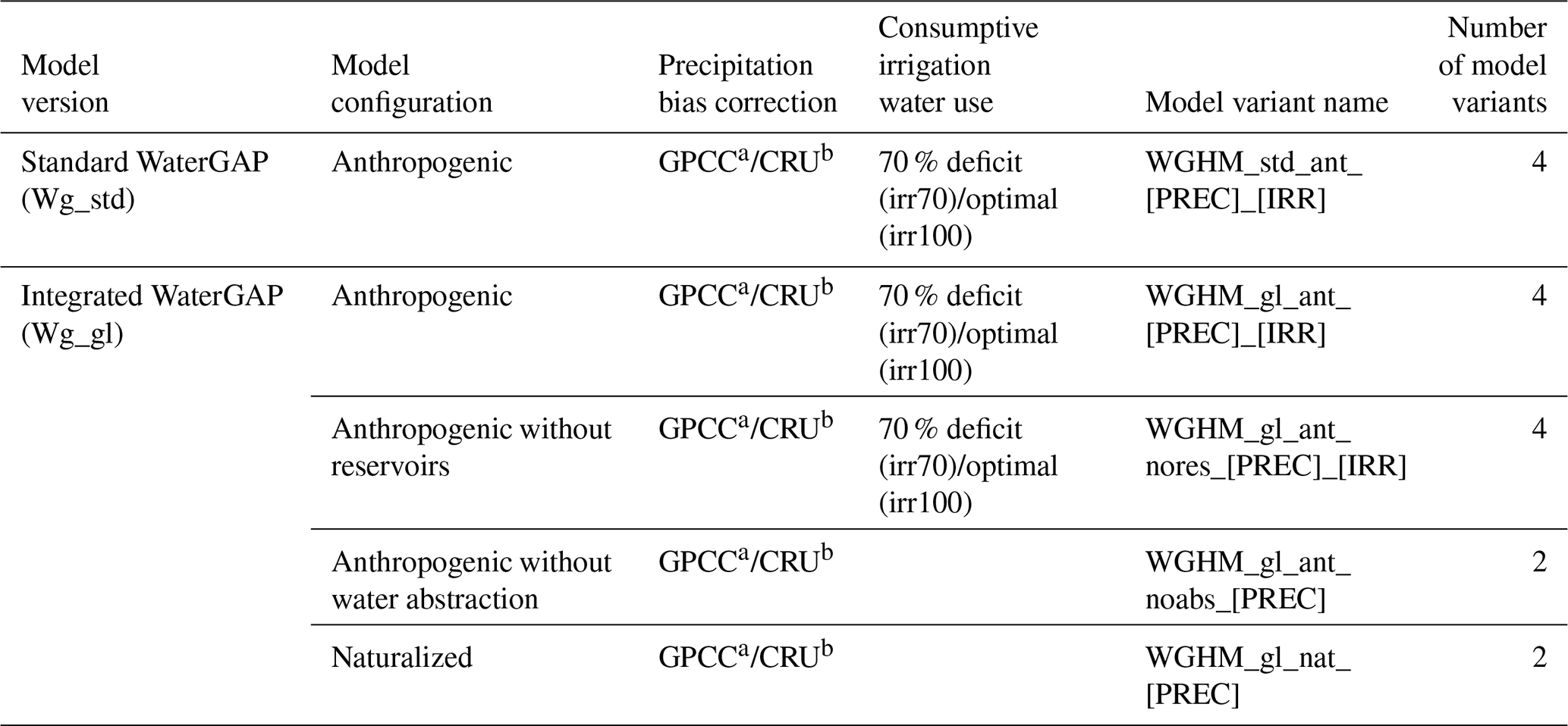
a Schneider et al. (2015). b Harris et al. (2014).
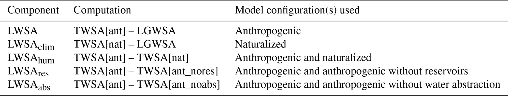
Table 2Overview of how the TWSA mass budget components were calculated using the integrated WaterGAP variants. TWSA[ant], TWSA[nat], TWSA[ant_nores] and TWSA[ant_noabs] were computed under the anthropogenic, naturalized, anthropogenic without reservoirs and anthropogenic without water abstraction configurations, respectively. The LGWSA remains unchanged.
In addition, we considered two different assumptions with respect to consumptive irrigation water use based on Döll et al. (2014). This flow is normally computed under the assumption that crops receive enough irrigation water to allow actual evapotranspiration to become equal to potential evapotranspiration (Döll et al., 2016). However, this is not always the case in regions affected by groundwater depletion where farmers may use less water due to water scarcity. Groundwater depletion is defined as a long-term decline in hydraulic heads and groundwater storage. Using a former version of WaterGAP, Döll et al. (2014) identified groundwater depletion areas worldwide by selecting the grid cells characterized by (1) an average groundwater depletion of at least 5 mm yr−1 over the period 1980–2009 and (2) an irrigation water abstraction volume of at least 5 % of total water abstraction volume. In this study, we either assumed that consumptive irrigation water use is optimal (i.e. that it corresponds to 100 % of the water requirement) or that it is equal to 70 % of the optimal level in these groundwater depletion areas (see optimal and 70 % deficit irrigation variants in Table 1).
3.1 Model evaluation
To evaluate the performance of GGM, simulated glacier mass changes of individual glaciers were compared to glacier observations (Sect. 3.1.1). Then, global mean TWSAs simulated by WaterGAP with and without the integration of GGM output were compared to GRACE observations (Sect. 3.1.2).
3.1.1 Comparison of observed and simulated annual and seasonal glacier mass changes
Comparison of observed average annual glacier mass changes for 31 glaciers with mostly decades of observations (Table S1) confirms the conclusion of Marzeion et al. (2012) that GGM is able to simulate annual glacier mass changes well. This study reveals that both average winter accumulation and summer melting are simulated reasonably too, but worse than the average annual mass changes, with Nash–Sutcliffe efficiencies NSE (Eq. 1; Nash and Sutcliffe, 1970) and correlation coefficients r being slightly lower than those of the annual values (Fig. 2). We also quantified, for each glacier, the fit between simulated and observed time series of winter and summer mass changes (two values per year times the number of years with observations). Approximately three-quarters of the glaciers have a NSE higher than 0.70 (Table S1), indicating a good model performance at the seasonal timescale even though GGM was only tuned with respect to the annual values. Only two glaciers, namely the Devon ice cap (Northwest Territories, Canada) and the Vernagtferner (Tyrol, Austria), show a negative NSE. The first is a marine-terminating ice cap where calving processes that are not modelled explicitly by GGM occur.
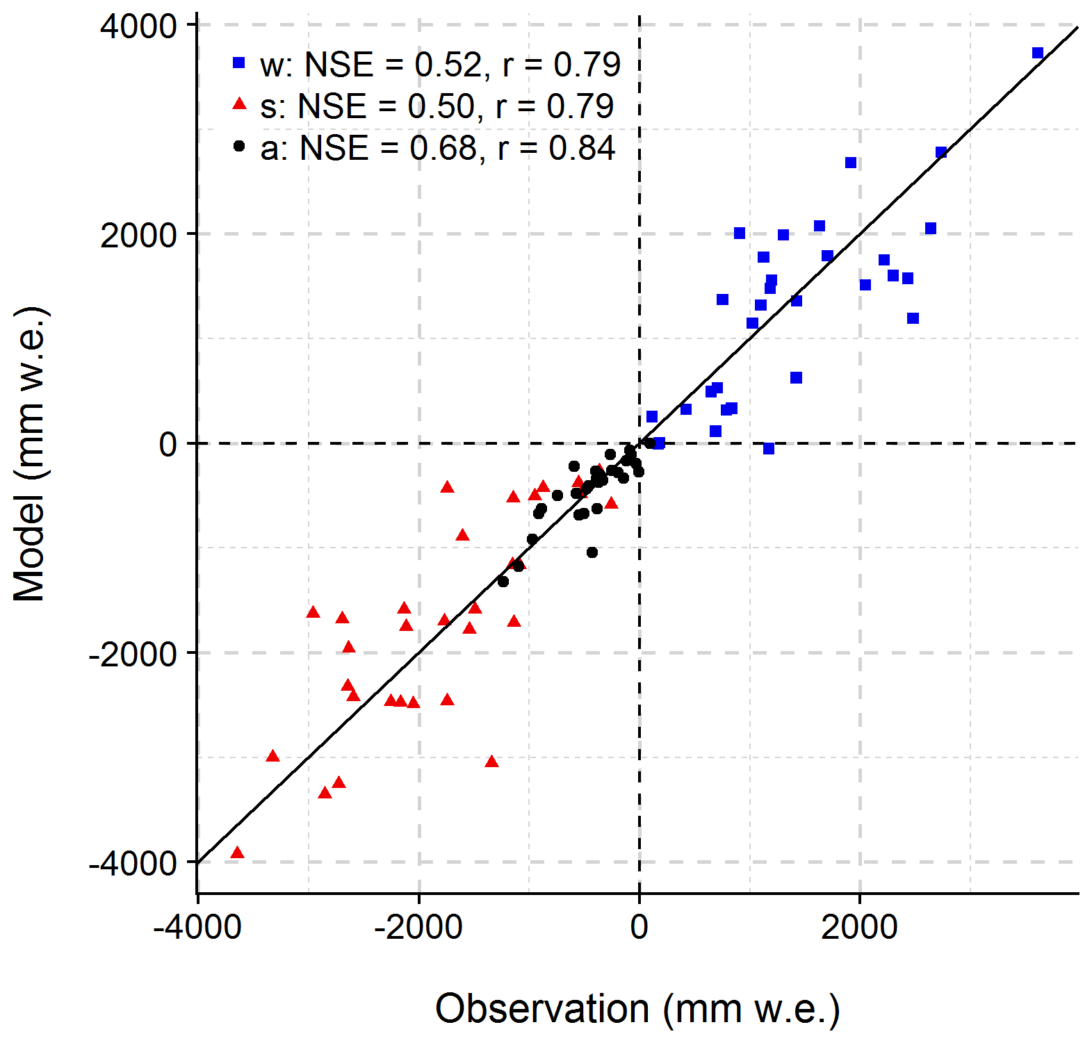
Figure 2Correlation between observed and modelled average annual, winter and summer glacier mass change. Observations were taken from the collections of the World Glacier Monitoring Service (31 glaciers included). Model results were obtained with the global glacier model of Marzeion et al. (2012). Nash–Sutcliffe efficiency (NSE) and correlation coefficient (r) values correspond to average annual (a), winter (w) and summer (s) mass changes. Millimetres of water equivalent (mm w.e.) are relative to glacier area.
3.1.2 Comparison of observed and simulated global mean TWSAs during January 2003 to August 2016
Figure 3a presents the time series of the ensemble of monthly TWSAs simulated by the standard (without glaciers) and the integrated (with glaciers) WaterGAP versions compared to GRACE observations. The NSE and r values shown in the figure were computed for the mean of the GRACE ensemble (consisting of four solutions) and the means of the Wg_std and Wg_gl ensembles (each ensemble consisting of the four anthropogenic variants; see Table 1). For both Wg_std and Wg_gl, there is a remarkably good fit between the modelled and the GRACE ensemble means in terms of NSE (0.85; 0.87) and r (0.92; 0.95), both of which reflect the good fit of the seasonal variability rather than of the trend. The fit is slightly better with Wg_gl, not only in terms of ensemble mean but also if we consider the NSE and r values obtained by comparing each individual GRACE solution to each individual WaterGAP solution (see Fig. S2 in the Supplement). With NSE around 0.80 during the period from January 2003 to December 2008, the fit is worse during the first 6 evaluation years than during the following period until August 2016 (Fig. 3a). Note, however, that the period from 2011 onwards contains more gaps in the GRACE data. Glaciers lead to a much stronger decreasing TWSA trend over the period considered. Monthly time series of LGWSA from GGM have a small seasonal variability and an almost linear decreasing trend (Fig. 3b). When adding LGWSA to the LWSA computed by Wg_std (Wg_std + GGM), the resulting time series of global mean values (purple ensemble in Fig. 3b) are indistinguishable from the TWSA time series computed by Wg_gl (green ensemble in Fig. 3a).
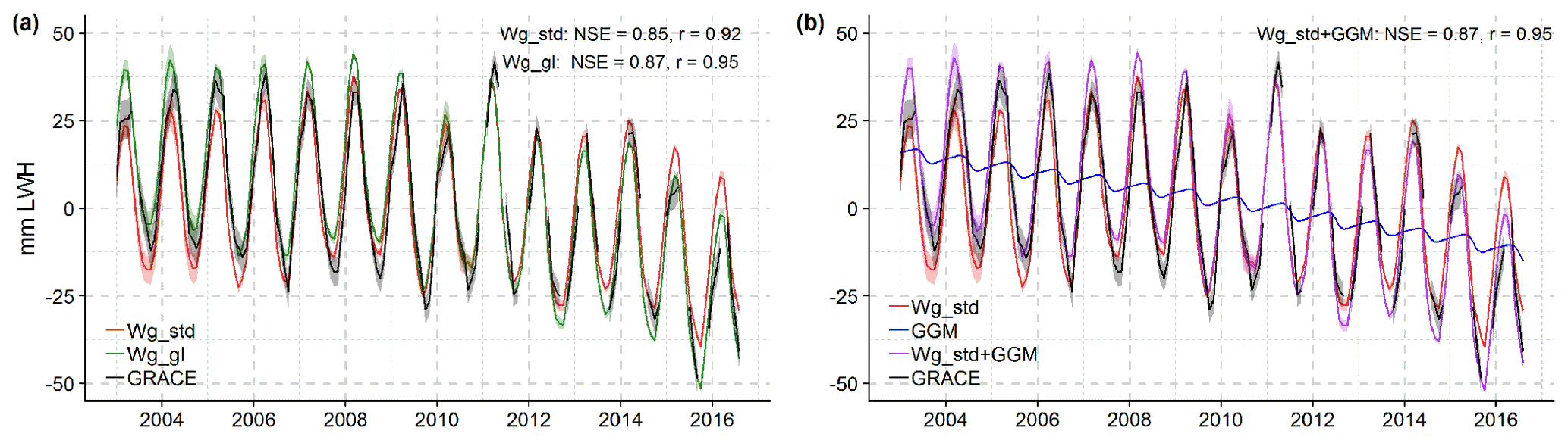
Figure 3Global mean monthly TWSA from GRACE observations and from different modelling approaches from January 2003 to August 2016. (a) TWSA from GRACE ensemble, LWSA from standard WaterGAP (Wg_std) in anthropogenic mode ensemble (Wg_std_ant_CRU_irr100, Wg_std_ant_CRU_irr70, Wg_std_ant_GPCC_irr100 and Wg_std_ant_GPCC_irr70 in Table 1) and TWSA from integrated WaterGAP (Wg_gl) in anthropogenic mode ensemble (Wg_gl_ ant_ CRU_ irr100, Wg_gl_ant_CRU_irr70, Wg_gl_ant_GPCC_irr100 and Wg_ gl_ant_GPCC_irr70 in Table 1). (b) TWSA from GRACE ensemble, LWSA from Wg_std ensemble as in (a), LGWSA from GGM and TWSA obtained by adding anomalies from Wg_std ensemble and GGM (Wg_std + GGM). For each ensemble, the curve represents the ensemble mean, and the shaded area around the curve represents either the uncertainty range (GRACE) or the ensemble range (Wg_std, Wg_gl and Wg_std + GGM). Nash–Sutcliffe efficiency (NSE) and correlation coefficient (r) obtained by comparing GRACE and model ensemble means are provided. Anomalies are relative to the mean over January 2006 to December 2015. Millimetres of land water height (mm LWH) are relative to the global continental area without the ice sheets (132.3×10⁶ km2).
To evaluate the WaterGAP performance separately, regarding its simulation of seasonality, trend and interannual variability, the original monthly TWSA time series (Fig. 3a) were decomposed (based on harmonic analysis) into de-trended, de-seasonalized and residual TWSAs (Fig. 4). Regarding seasonality, there is a remarkably good fit to GRACE with both Wg_std and Wg_gl; the seasonal amplitude and phase are very well reproduced by the models, even though for some years (e.g. 2003, 2004, 2011 and 2014) there seems to be a slight phase shift of approximately 1 month (Fig. 4a–b). The indicators show that the fit is very good with the two models and only slightly better for Wg_gl, reflecting the small contribution of glaciers to the seasonal variation of global mean TWSAs (NSE of 0.89 instead of 0.88 due to slightly increasing seasonal amplitude). The de-seasonalized time series show the strong impact of including glaciers into WaterGAP. Wg_gl can follow the negative trend of TWSAs observed by GRACE much better than Wg_std (Fig. 4c–d), and performance indicators are significantly higher (NSE improves from 0.65 to 0.74 and r from 0.85 to 0.93). However, the GRACE signal is overestimated before 2011 (in particular during 2007–2009) and in 2016 and underestimated in 2011. The overestimation during 2007–2009 may be partly due to a drought period in the Near East when a large number of new groundwater wells were drilled in this region, which is not taken into account in WaterGAP simulations of groundwater vs. surface water use (Döll et al., 2014). The residual signal present in the original time series (Fig. 4e–f), which includes the interannual variability, is very similar for the two models, which suggests that GGM does not contribute to the residual. With a NSE of 0.57, the fit of the residuals and, thus, simulation of interannual variability is relatively good but worse than for de-trended and de-seasonalized time series. The discrepancies to the GRACE signal follow the same pattern as in Fig. 4c–d. However, the fit to GRACE before 2007 is better than in de-trended and de-seasonalized time series.

Figure 4Temporal components of global mean monthly TWSA from GRACE observations and from two versions of WaterGAP2.2d from January 2003 to August 2016. GRACE ensemble, standard WaterGAP (Wg_std) ensemble (a, c, e) and integrated WaterGAP (Wg_gl) ensemble (b, d, f). (a, b) De-trended anomalies. (c, d) De-seasonalized anomalies (corresponding to linear and non-linear long-term variability). (e, f) Residual anomalies obtained by removing linear trend and seasonality (corresponding to non-linear interannual variability). For each ensemble, the curve represents the ensemble mean, and the shaded area around the curve represents either the uncertainty range (GRACE) or the ensemble range (Wg_std and Wg_gl). Nash–Sutcliffe efficiency (NSE) and correlation coefficient (r) obtained by comparing GRACE and model ensemble means are provided. Anomalies are relative to the mean over January 2006 to December 2015 and given in millimetres of land water height (mm LWH).
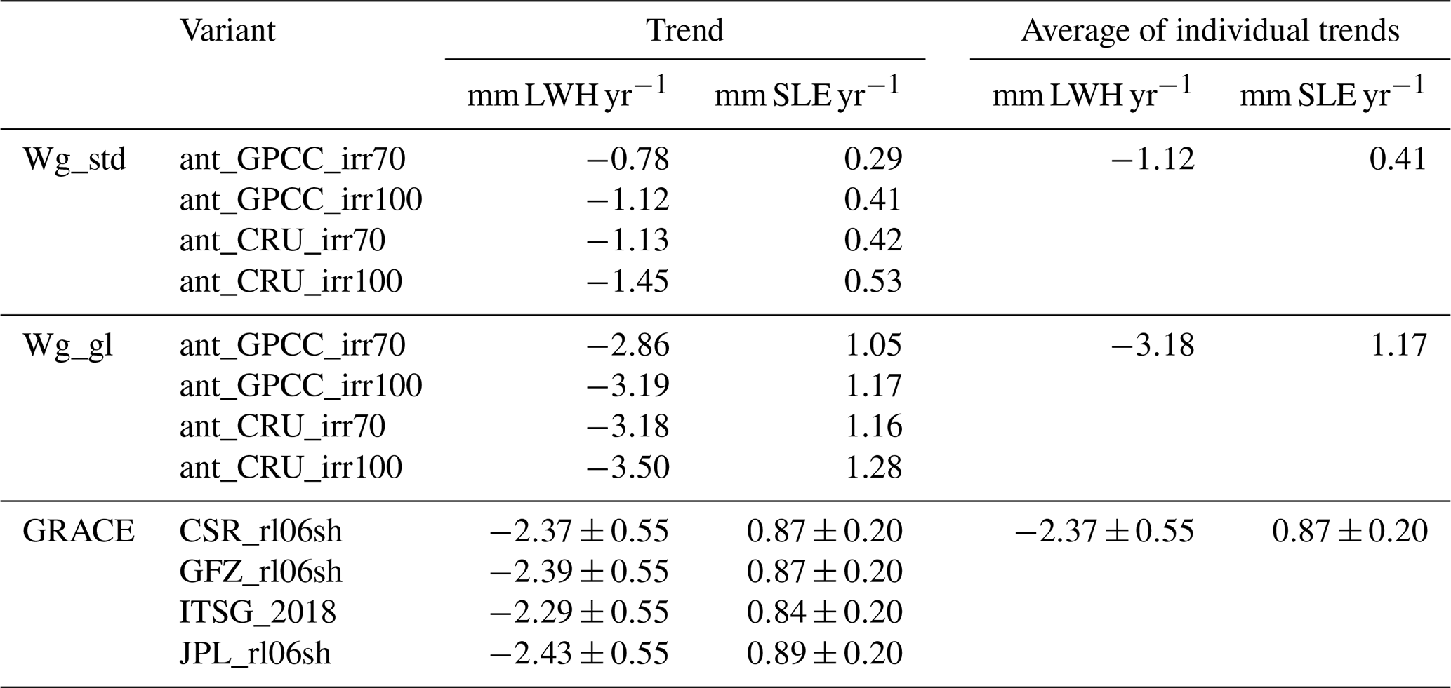
Linear trends are very sensitive to the selected time period and individual values. While the de-seasonalized TWSA from Wg_gl fits reasonably well overall to GRACE observations (Fig. 4d), Wg_gl considerably overestimates the trend determined for the time period of January 2003 to August 2016, if averaged over the four ensemble members, by about 30 % (Table 3). Wg_std variants underestimate the positive contribution to ocean mass change by about 50 %. Thus, the TWSA trend computed by integrating GGM output into WaterGAP results in a better estimation of the GRACE trend than if glaciers are neglected. Assuming 70 % deficit irrigation and utilizing GPCC precipitation, the simulated trend value of 1.05 mm SLE yr−1 is within the uncertainty bounds of the GRACE solutions (Table 3). The trend gets larger with optimal irrigation and CRU precipitation, which is mainly due to the larger TWSA values during the period 2003–2004 (Fig. 4d). The absolute difference between the two irrigation variants (0.11 to 0.12 mm SLE yr−1) is practically equal to the absolute difference between the two precipitation forcings (0.11 to 0.13 mm SLE yr−1); this means that, over this period, the trend is equally affected by the choice of irrigation variant than by the choice of precipitation forcing. The GRACE ensemble range is approximately 5 times smaller than the range of the Wg_std and Wg_gl ensembles. This is partly due to the choice of GRACE solutions; although coming from different processing centres, they were all corrected using the same GIA model (Caron et al., 2018). The trend spread owing to possible GIA models is reflected in the given standard uncertainty. The GIA model choice is the main contributor to uncertainty besides the GRACE Degree-1 correction.
Table 3Linear trends of TWSAs from GRACE observations and from WaterGAP2.2d from January 2003 to August 2016. Model estimates correspond to individual solutions of standard WaterGAP (Wg_std) and integrated WaterGAP (Wg_gl) ensembles. GRACE-derived estimates correspond to SH solutions from four processing centres (Center for Space Research – CSR; German Research Centre for Geosciences – GFZ; Institute of Satellite Geodesy – ITSG; and Jet Propulsion Laboratory – JPL). Trends were calculated according to the linear least squares regression method. Negative trends (mass loss) over the continents, expressed in millimetres of land water height (mm LWH, relative to the global continental area without the ice sheets 132.3×10⁶ km2), translate to positive trends (mass gain) over the oceans, expressed in millimetres of sea level equivalent (mm SLE, relative to the global ocean area 361.0×10⁶ km2).
Overall, we infer that integration of glacier model output into WaterGAP results in a better fit to GRACE in terms of linear trend, NSE and r for de-seasonalized time series, while simulated seasonality is barely improved. Seasonal variations of mean global TWSAs are simulated very well with Wg_gl compared to GRACE observations, interannual variability is captured to a certain extent and the linear trend is overestimated. The overall fit of the monthly time series of global mean TWSAs to GRACE (Fig. 3a) is remarkably good (NSE=0.87, r=0.95). Together with the positive evaluation of the glacier model results, this makes us confident that our modelling approach can be used to reconstruct TWSAs and, thus, the water mass transfer from the continents to the oceans for the time period before GRACE.
3.2 Global water transfer from continents to oceans over the period 1948–2016
3.2.1 Contribution of total continental water storage (TWSA)
Annual time series of global mean water storage anomalies over 1948–2016 were computed with integrated WaterGAP in anthropogenic mode (Fig. 5a). The continents lost between 93 and 111 mm LWH to the oceans between 1948 and 2016, equivalent to an ocean water mass increase of 34–41 mm SLE. Sea level rise is less pronounced in the case of less than optimal irrigation in groundwater depletion areas (variant_irr70, see Fig. 5b). While the 2003–2016 trends are equally affected by the precipitation data set and the irrigation assumption (Table 3), the 1948–2016 trends are much more strongly affected by the irrigation assumption than the applied precipitation data set (Fig. 5b). Continental water mass losses have been accelerating over time (see Tables 4 and S2) so that the 2003–2016 trends are approximately 6 times larger than the 1948–1975 trends.
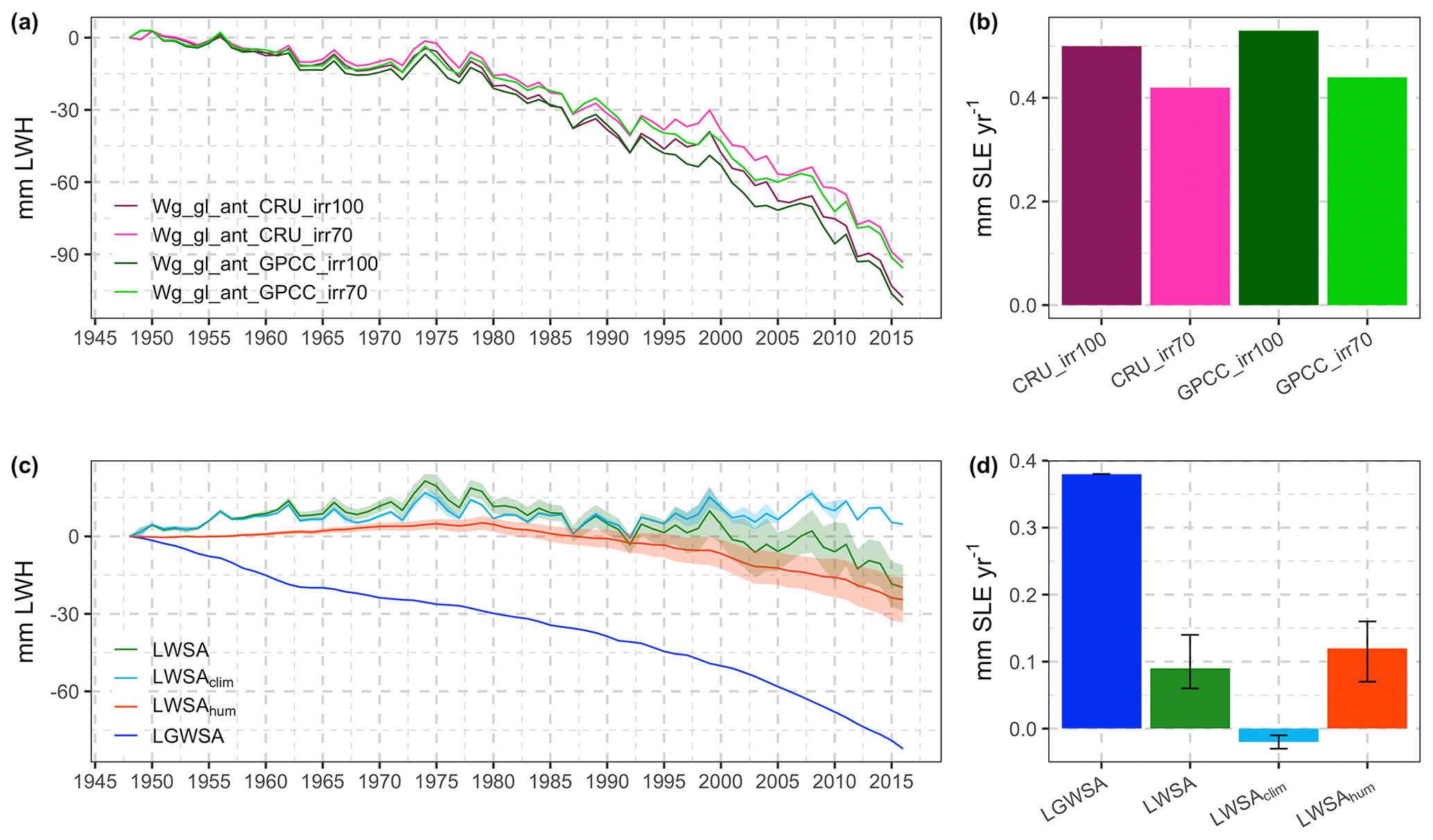
Figure 5Global annual TWSA and individual contributions from 1958 to 2016. TWSA was computed with four variants of integrated WaterGAP in anthropogenic mode (Table 1) and disaggregated into land glacier water storage anomaly (LGWSA) and land water storage anomaly (LWSA). LWSA was further disaggregated into anomalies of climate-driven land water storage anomaly (LWSAclim) and human-driven land water storage anomaly (LWSAhum). (a) Time series of TWSA and (b) corresponding linear trends of contribution of TWSAs to ocean mass change over 1948–2016. (c) Time series of LWSA, LWSAclim, LWSAhum and LGWSA (for each ensemble the curve represents the ensemble mean, and the shaded area around the curve represents the ensemble range) and (d) corresponding linear trends (ensemble ranges are represented as error bars). Anomalies are relative to the year 1948 and given in millimetres of land water height (mm LWH). Trends are given in millimetres of sea level equivalent per year (mm SLE yr−1); positive trends translate to ocean mass gain, whereas negative trends translate to ocean mass loss.
3.2.2 Contributions of glaciers (LGWSA), climate-driven land water storage (LWSAclim) and human-driven land water storage (LWSAhum)
Simulated TWSA (Fig. 5a–b) was disaggregated into its individual components LGWSA, LWSAclim and LWSAhum (Fig. 5c–d) using the results of the different Wg_gl model variants (Tables 1 and 2). Glacier mass loss is the dominant component of the TWSA mass budget (Fig. 5c–d), with LGWSA accounting for 81 % of the cumulated water mass loss from continents to oceans over 1948–2016. Overall, the contribution of LWSA to ocean mass change, which is dominated by its human-driven component (Fig. 5d), is also positive, representing 19 % of the cumulated water mass loss from continents. Interannual variability of LWSA stems from its climate-driven component (Fig. 5c). Trends of TWSA, LGWSA, LWSA, LWSAclim and LWSAhum show an acceleration in continental water mass loss over time (Table 4). However, note that LWSAclim and LWSAhum exhibit negative contributions to ocean mass change over the period 1948–1975, adding some water to the continents due to climate and human activities.
3.2.3 Contributions of reservoirs (LWSAres) and water abstraction (LWSAabs)
LWSAhum can be disaggregated into changes due to reservoir construction and operation (LWSAres) and changes due to human water abstraction (LWSAabs). Between 1948 and 2016, the continents gained approximately 22 mm LWH (i.e. 8 mm SLE) due to water impoundment in reservoirs and lost between 40 and 57 mm LWH (i.e. 15–21 mm SLE) due to water abstraction for human water use, resulting in an overall positive contribution of LWSAhum to ocean mass change (Figs. 5d and 6). However, continental water mass gain due to LWSAres more than compensated for the mass losses due to LWSAabs before 1980, when intensive reservoir construction led to a stronger increase in impounded water mass than afterwards (Fig. 6). Trends of LWSAres show a deceleration in continental mass gain due to water impoundment in reservoirs over time, whereas trends of LWSAabs show an acceleration in continental mass loss due to water abstraction (Table 4).
Table 4Linear trends of the contribution of TWSA, LGWSA, LWSA, LWSAclim, LWSAhum, LWSAres and LWSAabs to ocean mass change over 1948–1975, 1976–2002 and 2003–2016. Positive trends translate to ocean mass gain, whereas negative trends translate to ocean mass loss. Ensemble ranges are given in parentheses. Estimates are given in millimetres of sea level equivalent per year (mm SLE yr−1).
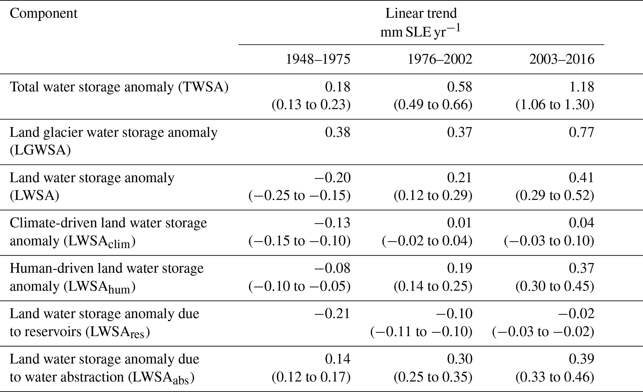
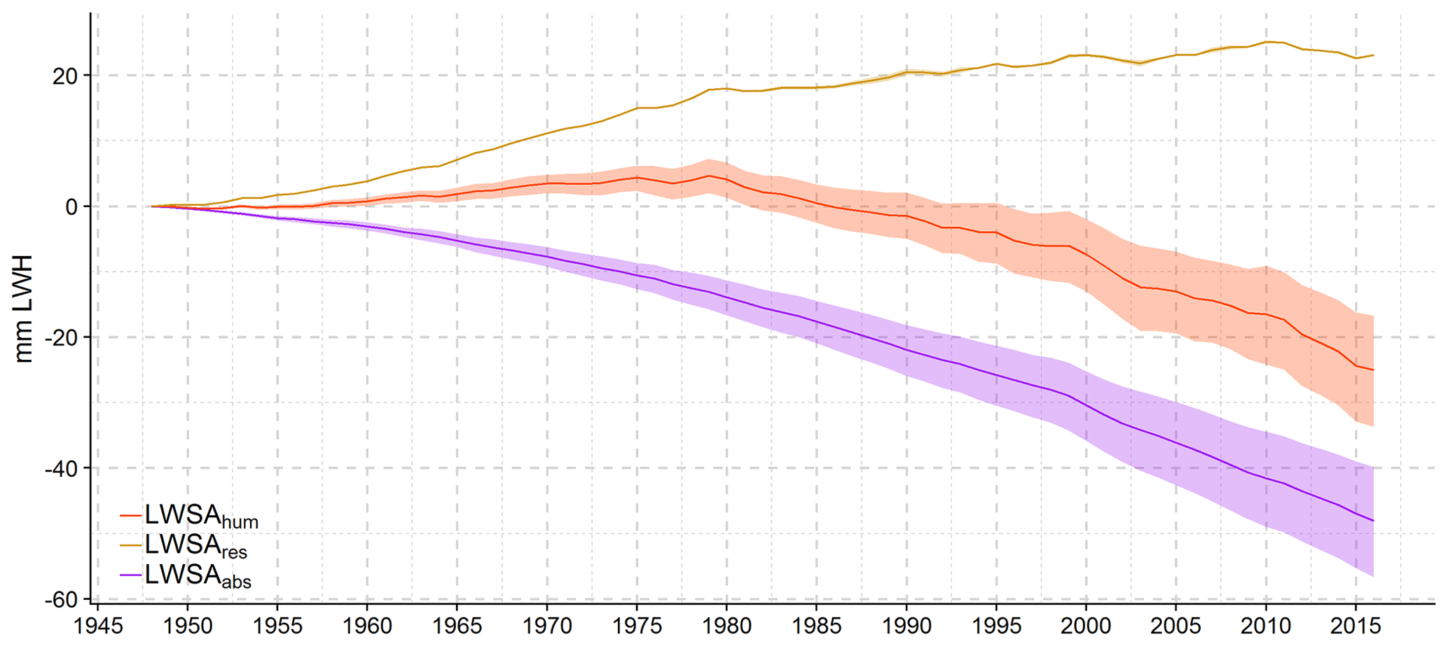
Figure 6Global mean annual human-driven LWSA and individual contributions from 1948 to 2016. Human-driven LWSA (LWSAhum; as in Fig. 5c) is disaggregated into anomaly due to reservoir operation (LWSAres) and water abstraction (LWSAabs). Anomalies are relative to the year 1948 and given in millimetres of land water height (mm LWH).
3.2.4 Relation between climate and land water storage
By comparing precipitation anomalies to LWSAclim, we found a correlation of r=0.63 with GPCC precipitation (Fig. 7, blue curves) and r=0.72 with CRU precipitation (Fig. 7, pink curves). Furthermore, we found a correlation of r=0.87 by comparing the difference between the two precipitation anomaly time series to the difference between the two LWSAclim time series. From these results, we deduced that precipitation is most likely the main driver of LWSAclim at the global scale.
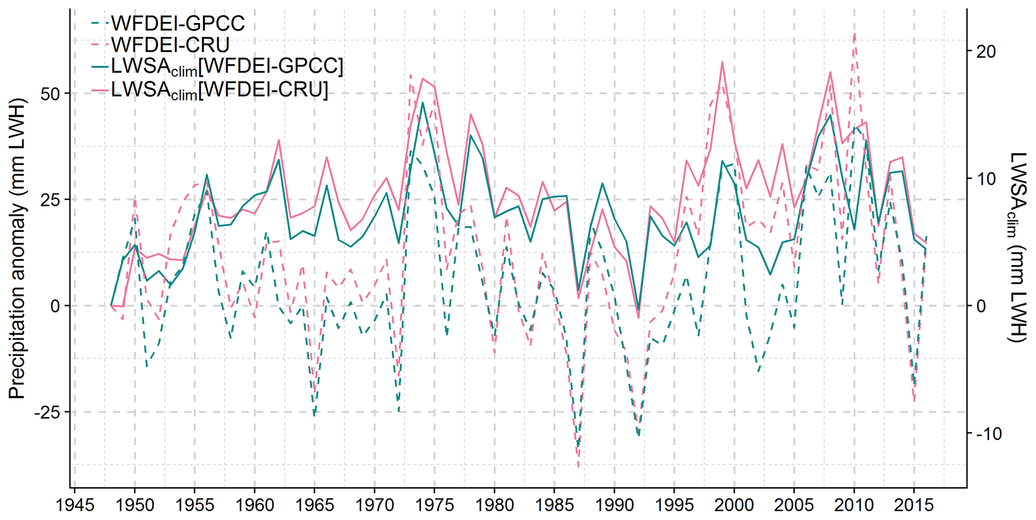
Figure 7Correlation between global annual climate-driven LWSA and precipitation anomaly from 1948 to 2016. Precipitation (rainfall plus snowfall) anomalies correspond to the WFDEI–GPCC and WFDEI–CRU forcings used in this study (Sect. 2.1.1). Climate-driven LWSA (LWSAclim[WFDEI-GPCC] and LWSAclim[WFDEI-CRU]) was obtained with the integrated WaterGAP in naturalized mode (see Table 2). Anomalies are relative to the year 1948 and given in millimetres of land water height (mm LWH).
Furthermore, given that previous studies have shown that LWSAclim is affected by internal multi-year climate variability such as ENSO (Cazenave and Llovel, 2010; Llovel et al., 2011; Cazenave et al., 2012; Boening et al., 2012), we also looked at the relation between the residual signal (i.e. non-linear interannual variability) in TWSAs (Fig. 8a) and short-term natural climate variability induced by ENSO and expressed as Multivariate ENSO Index (MEI) version 2 intensities (Wolter and Timlin, 1993; Wolter and Timlin, 1998) over 1980–2016 (Fig. 8b). The period was chosen according to the availability of MEI data. Based on the latter, we identified four major La Niña events (MEI<1) and five major El Niño events (MEI>1) during 1980–2016. According to our results, part of the signature in simulated TWSA interannual variability reflects ENSO-driven climate variability. We can observe a continental water storage decrease during El Niño phases that most certainly reflects the rainfall deficit over the continents (mostly the tropics) observed during this type of event, as opposed to a continental water storage increase during La Niña phases, as a response to increased rainfall. Differences due to precipitation input data are significant (Fig. 8a). The impact of the La Niña event of 1988–1989 is more prominent with GPCC precipitation; this is related to higher precipitation anomalies (i.e. wetter conditions) with GPCC (Fig. 7). The opposite is observed during the La Niña event of 1998–2000 and can be explained in the same way. Note that there is no difference between the two irrigation variants because LWSAhum mainly affects long-term linear variability (Figs. 5c and 6).
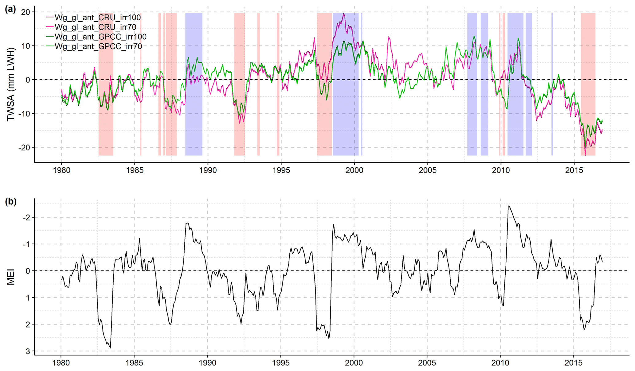
Figure 8Relation between global monthly TWSA and ENSO from January 1980 to December 2016. (a) Residual TWSA (non-linear interannual variability) computed with four variants of integrated WaterGAP (Wg_gl) in anthropogenic mode (Table 1). Anomalies are relative to the mean over January 1990 to December 2010 and given in millimetres of land water height (mm LWH). (b) Intensities in Multivariate ENSO Index (MEI) version 2 (produced by NOAA). Positive MEI values indicate El Niño and negative values indicate La Niña phases. El Niño (red) and La Niña (blue) phases are highlighted in the plot (a) whenever the MEI is larger than 1 or smaller than −1, respectively. Note the reversed vertical axis in (b).
3.2.5 Contributions of individual water storage compartments
Among the nine water storage compartments in Wg_gl, the largest absolute change over the period 1948–2016 is the mass loss from glaciers, i.e. a positive contribution of LGWSA to ocean mass change equivalent to 30 mm SLE (Fig. 9a). The second largest is groundwater depletion, with a decrease of 13–19 mm SLE, depending on the irrigation assumption. The third largest (with opposite sign) is water impoundment in reservoirs, which added 8 mm SLE to the continents. In the storage corresponding to surface water bodies (lake, reservoir, wetland and river), there are only very small differences due to the irrigation variant. Apart from the LGWSA, groundwater storage anomaly (GWSA) and reservoir water storage anomaly (ReWSA), the rest of the contributions are marginal, with negative contributions from the river and wetland storage and positive contributions from the soil, lake and snow storage (Fig. 9b). Differences related to precipitation forcing, which are more visible in Fig. 9b, exist in all the water storage compartments except for the glacier one, which is not affected by the different WaterGAP precipitation forcings as it is a direct input to WaterGAP.
4.1 TWSA temporal components
4.1.1 Linear trend: comparison to independent estimates
If we consider the linear trend of the ensemble mean, Wg_gl overestimates the positive contribution of TWSAs to ocean mass change by 30 %–50 % compared to the GRACE TWSA trends from this study (Tables 3 and 5). However, if we assume 70 % deficit irrigation in groundwater depletion regions and GPCC precipitation, the simulated trend is within the GRACE uncertainty bounds (Table 3). We consider this variant more likely because (1) GPCC is based on a much larger number of station records than CRU (see Fig. 2 of Schneider et al., 2014), and (2) it seems implausible that farmers in groundwater depletion areas have optimal irrigation conditions (Döll et al., 2014). Despite this, we included this assumption in the design of the model variants as an upper bound of groundwater depletion (Fig. 9). GRACE estimates from other studies (Rietbroek et al., 2016; Reager et al., 2016; Blazquez et al., 2018) suggest much smaller continental water mass losses to oceans (Table 5). Differences between GRACE-based TWSA trends from this study and from independent sources are of the same order of magnitude as the differences between GRACE- and model-based TWSA trends from this study. This suggests that GRACE-based TWSA trends are very sensitive to the multiple processing parameters applied to the GRACE Level-2 data (Blazquez et al., 2018).
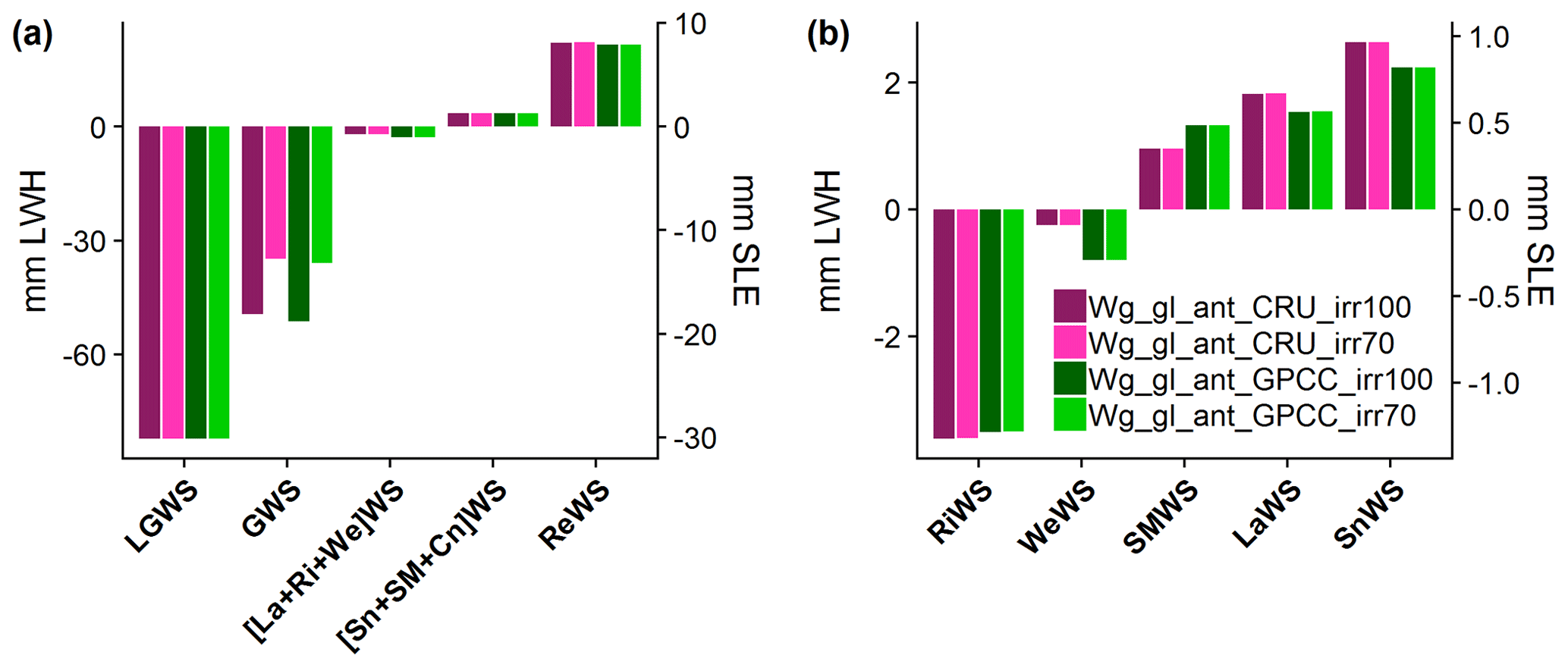
Figure 9Global cumulated water storage change in individual water storage compartments from 1948 to 2016. Estimates were obtained with four variants of integrated WaterGAP in anthropogenic mode (Table 1). (a) Water storage (WS) change in glacier (LG), groundwater (G), aggregate of lake (La), river (Ri) and wetland (We), aggregate of snow (Sn), soil moisture (SM) and canopy (Cn) and reservoir (Re) compartments. (b) Water storage change in river, wetland, soil moisture, lake and snow storage. Canopy storage is not included because the cumulated change is of the order of mm LWH. Estimates are given in millimetres of land water height (mm LWH) and of sea level equivalent (mm SLE).
Table 5Comparison between trends of TWSA, LGWSA, LWSA, LWSAhum and LWSAclim from the literature and this study (in parentheses). TWSA trends from this study were derived from GRACE observations and integrated WaterGAP (Wg_gl) in anthropogenic mode. LWSA trends were obtained by subtracting LGWSA trends from TWSA trends based on either GRACE or Wg_gl. LWSAclim trends were obtained by subtracting LWSAhum based on Wg_gl from LWSA, based on either GRACE or Wg_gl. Positive trends translate to ocean mass gain, whereas negative trends translate to ocean mass loss. Estimates are given in millimetres of sea level equivalent per year (mm SLE yr−1).
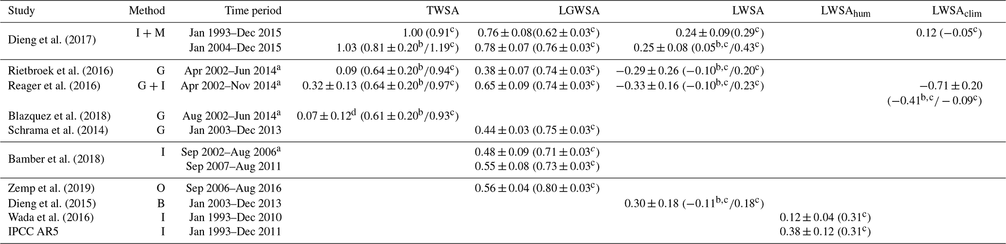
a Only three (CSR_rl06sh, ITSG_2018 and JPL_rl06sh) out of four GRACE solutions were considered (GFZ_rl06sh was excluded because of a lack of values in 2002). b Trends based on GRACE data sets used in this study. c Trends based on modelled data sets (Wg_gl) used in this study. d Uncertainty estimates in the source paper are expressed in 1.65σ. Here, they are expressed in 1σ. Note: I – multiple independent estimates; M – modelling; G – GRACE data; O – observations; and B – global water mass budget.
The overestimation of the TWSA positive contribution by Wg_gl may arise from uncertainty in both the LWSA and LGWSA components. There is a rather good agreement between LGWSA trends from GGM, on the one hand, and from Dieng et al. (2017) and Reager et al. (2016), on the other hand. The agreement to Dieng et al. (2017) is not surprising, since their estimates were obtained by averaging three data sets, including a GGM data set used by Marzeion et al. (2015; update from Marzeion et al., 2012). Nevertheless, according to the GRACE-based estimates from Rietbroek et al. (2016) and Schrama et al. (2014), GGM overestimates the LGWSA contribution. The more recent non-GRACE-based estimates from Bamber et al. (2018) and Zemp et al. (2019) are in better agreement with the estimates from GGM, even though they are still too small in comparison (Table 5).
The discrepancy between GRACE- and model-based TWSA trends from this study is also reflected in the LWSA trends. If LGWSA is subtracted from TWSA of Wg_gl, a mass loss on land is computed, while a (small) mass gain on land results if GRACE-based TWSA is used instead (Table 5). This can be related to the findings of Scanlon et al. (2018), which show that LWSA trends summed over 183 basins worldwide (∼63 % of global continental area excluding the ice sheets) indicate a mass gain on land for GRACE but a mass loss on land for models. The LWSA trends from Rietbroek et al. (2016) and Reager et al. (2016) suggest a higher water mass gain on continents than our GRACE-based trends, reflecting the discrepancy in TWSA trends, which is not compensated by smaller glacier mass losses in these two studies. On the other hand, it is noteworthy that our model-based LWSA trends are in good agreement with other non-GRACE-based trends, namely the ones from Dieng et al. (2015) and Dieng et al. (2017); see Table 5..
The presumed overestimation of the LWSA positive contribution to ocean mass change by Wg_gl may reflect an overestimation of the LWSAhum positive contribution and/or an underestimation of the LWSAclim negative contribution. Our LWSAhum trend is in good agreement with the one reported by the IPCC AR5 but overestimated according to the trend of Wada et al. (2016); see Table 5. Wada et al. (2016) argued that the LWSAhum positive contribution of the IPCC AR5 is probably overestimated by a factor of 3, and that this is partly due to the fact that the IPCC AR5 assumes that 100 % of groundwater depletion ends up in the ocean, whereas their study shows that only 80 % of it actually does. We estimate a groundwater depletion trend of 0.39 mm SLE yr−1 over 2003–2016 (see Table S3), which is within the uncertainty bounds of the trend reported by Wada et al. (2016), i.e. 0.30±0.10 mm SLE yr−1 over 2002–2014, even if it is slightly higher. Concerning the LWSAclim component, Dieng et al. (2017) computed a positive contribution, whereas Wg_gl computed a negative contribution, suggesting differences between models. Moreover, the trend from Reager et al. (2016) suggests that Wg_gl underestimates continental water mass gain due to climate variability; by assuming GRACE-based TWSA, we obtain a more negative LWSAclim trend; however, this still differs from the estimate of Reager et al. (2016) by roughly a factor of 2 (Table 5).
4.1.2 Seasonality and interannual variability
The small discrepancy between GRACE and Wg_gl in terms of TWSA seasonality (Fig. 4b) is partly due to differences in seasonal amplitude. For instance, some years (2006, 2009 and 2011) show smaller simulated seasonal amplitude than what is observed by GRACE. Although we did not investigate this matter at a regional scale, we speculate that this might be due to a systematic underestimation of seasonal amplitude in tropical basins by WaterGAP, where the seasonal signal is strongest, resulting from insufficient storage capacity (Scanlon et al., 2019). At a global scale, however, underestimation in tropical basins might be compensated by overestimation in other types of basins.
The most prominent discrepancies between global mean monthly TWSAs from GRACE and Wg_gl are observed in the residual signal, which contains the interannual variability (Fig. 4f). The interannual variability comes almost completely from the LWSA component (Fig. 4e–f) and, more specifically, from its climate-driven component (LWSAclim in Fig. 5c) at a global scale. WCRP (2018) pointed out that this is arguably the most difficult component in the land water budget to quantify. Humphrey et al. (2016) show that interannual anomalies in the GRACE signal can be correlated to anomalies in precipitation (positive correlation) and near-surface temperature (negative correlation); our results confirm the positive correlation to precipitation (Fig. 7). The discrepancy between the residual signal in GRACE and Wg_gl is more prominent in some years (Fig. 4f). This may reflect the occurrence of ENSO events; in particular, we can identify the intense La Niña event of 2010/2011 and the intense El Niño event of 2015/2016. If we rely on the validity of the GRACE time series, despite the significant gaps in the data for both events, then it can be inferred that, even though Wg_gl reproduces the events to some extent, it underestimates their intensity. By studying the GRACE record at a regional scale, Wang et al. (2018) showed that the sensitivity to ENSO modulations is more prominent in the global exorheic (i.e. draining into the ocean) system as opposed to the global endorheic (i.e. landlocked) system (see their Fig. 2). Within the exorheic system, tropical basins (particularly the Amazon) are more sensitive to these modulations (Llovel et al., 2011). This suggests the difficulty in correctly simulating not only seasonal (Scanlon et al., 2019) but also annual amplitudes in tropical basins by WaterGAP.
4.2 Limitations of study
Simulated global TWSA is the result of aggregating water storage change estimates corresponding to nine individual water storage compartments and 64 432 grid cells. There is uncertainty in each single estimate (due to uncertain climate input, assumptions related to water use, model parameters, etc.). However, errors in individual storage compartments and at smaller spatial scales may average out once aggregated at a global scale. In this section, we discuss the limitations of our reconstruction of global TWSA time series and, thus, mass transfer from continents to oceans. Limitations in our approach are related to the integration of glacier data as an input to WaterGAP, to the global models (GGM and WaterGAP) used to compute LGWSA and LWSA and to missing components that were not accounted for in this study.
4.2.1 Glacier data integration approach
The glacier data integration significantly improved the simulation of the global mean TWSA linear trend by WaterGAP (Fig. 4c–d). However, this approach does not give appreciably different results from simply adding the separately estimated LGWSA and LWSA components (hereafter the addition approach) at a global scale (Fig. 3). According to the data used in this study, we estimate that glaciers cover 0.38 % of the global continental area (excluding the ice sheets), which is smaller than the estimate of Bamber et al. (2018), amounting to 0.50 %. However, the area effectively accounted for by integrated WaterGAP amounts to 0.34 % (∼11 % of global glacier area is neglected; see Sect. 2.3.1), resulting in a reduction in its global land area ranging from 0.39 % in 1948 to 0.34 % in 2016. Thus, it is not strange that the reduction in the land area had an insignificant effect at a global scale. We speculate that, at a basin scale, the glacier data integration approach might show significantly different results from the addition approach.
Moreover, our approach has limitations regarding the fate of the internally calculated glacier runoff. One of the sources of uncertainty related to the contribution of glaciers to sea level rise is the interception of glacier runoff by land; it is still widely assumed that glacier runoff flows directly to the ocean, with no delay from or interception by water storage compartments (Church et al., 2013). In our approach, we assume that glacier runoff is intercepted by surface storages but not by subsurface (soil and groundwater) storages. We made this assumption because we have no means of assessing how much glacier runoff is intercepted by subsurface storages at a global scale.
4.2.2 Global modelling of LGWSA
Previous studies (Marzeion et al., 2015; Slangen et al., 2017) have shown agreement between GGM and other global glacier models. For instance, according to Marzeion et al. (2015), the reconstruction of global glacier mass change during the 20th century by GGM is consistent with the ones obtained from other methods of reconstruction (see their Fig. 1). However, note that this might simply mean that the methods are consistently wrong. In addition, using an extrapolation of glaciological and geodetic observations, Zemp et al. (2019) estimate that glaciers (apart from the ice sheets) contributed 23±14 mm SLE to global mean sea level rise from 1961 to 2016. We estimate a contribution of 25 mm SLE with GGM over the same period, which is remarkably consistent with the estimate from Zemp et al. (2019). Furthermore, our evaluation of GGM performance (Sect. 3.1.1) shows that this model can reproduce the observed mean seasonality of winter accumulation and summer ablation well; this is not always the case for global glacier models (Fig. 4; Hirabayashi et al., 2010).
Despite the fact that we consider GGM estimates to be state of the art, they are subject to multiple sources of uncertainty. Input data (climate forcing and glacier outlines), simplification of physics in the model, observation data used for calibration and the calibration itself are among the main sources. GGM includes uncertainty estimates related to annual glacier mass change time series. However, we did not include these uncertainty estimates in our assessment (we only included the trend uncertainty, which corresponds to a 1σ standard uncertainty) for consistency reasons (i.e. most data sets used for the assessment have unknown uncertainties).
4.2.3 Global modelling of LWSA
Uncertainty in WaterGAP estimates is related to both the LWSAhum and LWSAclim components. Modelling of groundwater depletion, which is both related to climate variability and human water use, is of key importance, as global water storage trends computed with WaterGAP are particularly sensitive to these variations (Müller Schmied et al., 2014). Global groundwater depletion is highly linked to irrigation groundwater abstraction. The estimation of gross and net irrigation groundwater abstraction is not a trivial task, as it relies mainly on statistical data and assumptions and depends on climate input (Döll et al., 2016). Siebert et al. (2010) estimated that 43 % of the total consumptive irrigation water use comes from groundwater. The rate of global groundwater depletion has been subject to much debate (Döll et al., 2014; Wada et al., 2017). According to Wada et al. (2017), most studies likely overestimated the cumulative contribution of groundwater depletion to global sea level rise during the 20th and early 21st century. Our groundwater depletion estimates are very likely overestimated under optimal irrigation; however, they are more robust under 70 % deficit irrigation (Döll et al., 2014). Our estimate of 0.32 mm SLE yr−1 over 2003–2016 under 70 % deficit irrigation (see Table S3) is in good agreement with the study of van Dijk et al. (2014), who estimated a trend of 0.26 mm SLE yr−1 over 2003–2012 using a data assimilation framework to integrate water balance estimates from GRACE and several GHMs.
Modelling reservoir storage and operation is also subject to multiple sources of uncertainty (e.g. quality of reservoir database, algorithms and assumptions used in model). In the present study, we did not include model variants differing from one another in the way reservoirs are handled. Wada et al. (2017) estimated a global reservoir storage capacity of 7968 km3 (∼22 mm SLE) until 2014. WaterGAP has a global reservoir storage capacity of 5764 km3 (∼16 mm SLE), as it only simulates the largest 1082 artificial reservoirs (Sect. 2.1.1). Furthermore, by assuming that on average 85 % of the reservoir capacity is used, and taking into account seepage (i.e. adding additional water that seeps underground), Wada et al. (2017) estimated a potential total water impoundment in reservoirs of ∼29 mm SLE. Upon application of the reservoir operation algorithm implemented in WaterGAP, we estimate an actual total water impoundment of ∼10 mm SLE, which corresponds to roughly 63 % of the global reservoir capacity. Wada et al. (2017) might overestimate the additional water due to seepage and the fraction of the design capacity that is in reality filled (85 % according to their assumption). However, the estimate in our study is likely an underestimation of the impoundment of water in artificial reservoirs because WaterGAP only simulates the largest reservoirs and does not account for seepage. In addition, WaterGAP incorporates the reservoirs from the GRanD v1.1 database but not the additional ones from the new GRanD v1.3 release (http://globaldamwatch.org, last access: 17 April 2020). GRanD v1.3 includes 458 additional reservoirs compared to GRanD v1.1. Out of 458 reservoirs, 447 were put in operation between 1948 and 2016. Out of these 447 reservoirs, 173 have a total capacity of at least 0.5 km3 and, thus, would be simulated as reservoirs by WaterGAP. The cumulated total capacity of these 173 reservoirs amounts to 599 km3. The remaining 274 smaller reservoirs have a cumulated total capacity of 62 km3. Out of the 173 large reservoirs, 164 were put in operation between 2000 and 2016. Taking into account that we computed an actual total water impoundment of roughly 63 % of the global reservoir capacity, we can infer that incorporating the additional large reservoirs would lead to an additional impoundment of 378 km3 (1.05 mm SLE) over 1948–2016, thus increasing the total impoundment of water from 8 to 9 mm SLE, i.e. from 22 to 25 mm LWH (compare Fig. 6). Most of the additional impoundment not taken into account in this study (369 km3, 1.02 mm SLE) occurred in the period 2000–2016. Therefore, WaterGAP is expected to overestimate the positive contribution of water storage on continents during the GRACE period by approximately 0.06 mm SLE yr−1, which explains part of the overestimation as compared to GRACE (Table 3).
LWSAclim is largely affected by uncertain climate input data. As stated by Döll et al. (2016), this remains one of the main challenges in the development and application of GHMs. Precipitation and radiation data have been identified as strong drivers of water storage change (Müller Schmied et al., 2014, 2016; Humphrey et al., 2016). Our assessment accounts for part of the uncertainty related to precipitation input data by considering two different climate forcings (WFDEI–GPCC and WFDEI–CRU). By comparing global precipitation anomalies from CRU TS3.10 and GPCC v5, Harris et al. (2014) identified a correlation of r=0.88 over 1951–2009 (see their Table II and Fig. 10). We identified a correlation of r=0.86 over 1948–2016 between the precipitation time series used in this study. Note that the high correlation between the two data sets means that our ensemble underestimates the uncertainty in global TWSAs due to precipitation input data. However, in general we believe that WFDEI–GPCC is likely to be more reliable than WFDEI–CRU because (1) the monthly time series of gridded precipitation from GPCC used to bias adjust WFDEI–GPCC are based on more observation stations (Müller Schmied et al., 2016), and (2) GRACE-derived trends of TWSAs in 186 large river basins correlate much more with trends computed by WaterGAP if GPCC precipitation is used (Scanlon et al., 2018). Despite this, both forcings are not well suited for trend analysis as a consequence of the bias correction, which significantly affects trends of climatic variables such as temperature and precipitation (Hempel et al., 2013; Weedon et al., 2014). TWSA trends simulated by WaterGAP are most likely affected by this caveat regarding the climate forcing. Moreover, note that, given the complex interactions and feedbacks in the climate system, we could not, unlike for LWSAhum, isolate the different components of LWSAclim.
4.2.4 Missing components
The Caspian Sea (the largest endorheic lake worldwide), which was one of the largest contributors to global lake water storage loss during the 20th century (Milly et al., 2010), is missing from our assessment because the WaterGAP model grid, based on the WATCH-CRU land–sea mask, does not include it. Its contribution to sea level rise, if a complete loss to oceans via vapour transfer is assumed, was previously estimated to be 0.06 mm SLE yr−1 over 1992–2002 (Milly et al., 2010) and 0.071±0.006 mm SLE yr−1 over April 2002–March 2016 (Wang et al., 2018), including only surface water variations, and 0.109±0.004 mm SLE yr−1 over 2002–2014 (Wada et al., 2017), including variations in both surface water and the influenced groundwater. The GRACE-based solutions used in this study consider the Caspian Sea as a lake and do include its mass changes. Our net loss estimates from lake surface integration amount to 0.055±0.003 mm SLE yr−1 (fit uncertainty) over 2003–2016, on average over all four solutions (see Figs. S3 and S4), plus an unassessed leakage contribution (∼20 %). Note that, during the GRACE period, the underestimation of modelled mass loss on continents due to the missing Caspian Sea is almost compensated (in terms of linear trend) by the underestimation of modelled mass gain due to the missing reservoirs from GRanD v1.3 (Sect. 4.2.3).
Moreover, WaterGAP does not account for land cover change. This means that the impact of human-induced phenomena such as deforestation is neglected. Wada et al. (2017) estimated that net global deforestation contributed ∼0.035 mm SLE yr−1 to sea level rise over 2002–2014 through runoff increase and water release from oxidation and plant storage. Using a dynamic global vegetation and water balance model, Rost et al. (2008) estimated that human-induced land cover change (mainly deforestation) reduced evapotranspiration by 2.8 % and increased streamflow by 5.0 % globally over 1971–2000.
In order to quantify water transfers between continents and oceans over 1948–2016, we used a non-standard version of WaterGAP that is able to simulate the variations in all continental water storage compartments. The model was run under different assumptions of irrigation water use and with different precipitation input data sets to account for major hydrological modelling uncertainties. Time series of global mean monthly TWSAs simulated with this ensemble were evaluated by comparing them to estimates from an ensemble of GRACE solutions over January 2003 to August 2016. A remarkable agreement between observed and modelled global mean monthly TWSA time series was found, with a high agreement with respect to seasonality and a likely small overestimation of the water storage decline for which a clear identification of the specific causes remains difficult due to the complex feedback in the modelling system. On the other hand, Gutknecht et al. (2020) have demonstrated that replacing standard Degree-1 coefficients with individual solutions during GRACE data processing can result in trends up to 0.3 mm SLE yr−1 stronger than shown here.
According to our model-based reconstruction, we conclude that continental water mass loss resulted in an ocean mass gain equivalent to 34–41 mm SLE during 1948–2016. Continents (including glaciers) lost water at an accelerated rate over time, with a contribution to ocean mass change of 0.18 mm SLE yr−1 over 1948–1975, 0.58 mm SLE yr−1 over 1976–2002 and 1.18 mm SLE yr−1 over 2003–2016 (Table 4). Global glacier mass loss accounted for 81 % of the cumulated mass loss over 1948–2016, while the remaining 19 % was lost from other continental water storage compartments (LWSAs). LWSAs over 1948–2016 were dominated by the impact of direct human interventions, namely water abstractions and the impoundment of water in reservoirs. Continental mass loss due to water abstractions (15–21 mm SLE), mainly driven by irrigation water demand, showed an acceleration over time, with water lost mainly from groundwater (13–19 mm SLE). This mass loss offset continental mass gain from reservoir water impoundment (>8 mm SLE), which showed a deceleration over time. Climate-driven LWSAs are highly correlated to precipitation anomalies and is also influenced by multi-year modulations related to ENSO.
Significant uncertainty in our assessment arises from the simulation of human-driven LWSAs. Modelling of groundwater depletion, which is highly sensitive to irrigation water use assumptions, and of reservoir storage and operation is particularly challenging. Furthermore, simulated climate-driven LWSAs are affected by uncertainty in the climate input data. Despite the limitations of our model-based approach and the remaining challenges, our assessment gives valuable insights on the main individual mass components and drivers of global water transfers from continents to oceans and on possible routes for model improvement. More research is required to better constrain the simulation of human water use in GHMs. Finally, future research should go beyond the global scale by identifying the main regions contributing to water transfers between continents and oceans.
All GRACE-based and model-based data sets used in this study are available upon request from the corresponding author. The glacier surface mass balance observational data used in this study are publicly available and can be downloaded from https://wgms.ch/products_ref_glaciers/ (last access: 18 April 2018; World Glacier Monitoring, 2018). The MEI data used in this study are publicly available and can be downloaded from https://www.esrl.noaa.gov/psd/enso/mei/data/meiv2.data (last access: 10 July 2019; NOAA Physical Sciences Laboratory, 2019).
The supplement related to this article is available online at: https://doi.org/10.5194/hess-24-4831-2020-supplement.
PD and DC designed the study. DC conducted background research, implemented the computer code for the integrated WaterGAP model version, conducted model simulations, prepared the WaterGAP data, performed the formal analysis and drafted the initial paper, with substantial revisions from PD. BDG, BM, HMS and PD discussed the results and edited the initial paper. BDG prepared the GRACE data, provided a script for the computation of linear trends and the temporal disaggregation of TWSA time series and contributed to the analysis of GRACE-based TWSAs. PD contributed to the analysis of model-based TWSAs and individual components. BM provided GGM simulation data and contributed to the analysis of glacier mass changes. HMS supported the implementation of the computer code and provided a script for the aggregation of model-based TWSAs over the global continental area. JHM prepared the gridded glacier-related data.
The authors declare that they have no conflict of interest.
We thank Tim Trautmann from the Institute of Physical Geography of the Goethe University Frankfurt and the two anonymous reviewers for their valuable and constructive comments, which significantly helped in improving the quality of this paper. We also thank the investigators of the World Glacier Monitoring Service network and the NOAA Earth System Research Laboratory's Physical Sciences Division for free and open access to their data sets.
This research has been supported by the European Space Agency (ESA) through its Sea Level Budget Closure CCI project (grant no. 4000119910/17/I-NB).
This paper was edited by Giuliano Di Baldassarre and reviewed by two anonymous referees.
Bahr, D. B., Meier, M. F., and Peckham, S. D.: The physical basis of glacier volume-area scaling, J. Geophys. Res., 102, 20355–20362, 1997.
Bamber, J. L., Westaway, R. M., Marzeion, B., and Wouters, B.: The land ice contribution to sea level during the satellite era, Environ. Res. Lett., 13, 063008, https://doi.org/10.1088/1748-9326/aac2f0, 2018.
Bergmann-Wolf, I., Zhang, L., and Dobslaw, H.: Global eustatic sea-level variations for the approximation of geocenter motion from grace, J. Geod. Sci., 4, 37–48, https://doi.org/10.2478/jogs-2014-0006, 2014.
Blazquez, A., Meyssignac, B., Lemoine, J. M., Berthier, E., Ribes, A., and Cazenave, A.: Exploring the uncertainty in GRACE estimates of the mass redistributions at the Earth surface: implications for the global water and sea level budgets, Geophys. J. Int., 215, 1, 415–430, https://doi.org/10.1093/gji/ggy293, 2018.
Boening, C., Willis, J. K., Landerer, F. W., Nerem, R. S., and Fasullo, J.: The 2011 La Niña: So strong, the oceans fell, Geophys. Res. Lett., 39, 19, L19602, https://doi.org/10.1029/2012GL053055, 2012.
Caron, L., Ivins, E. R., Larour, E., Adhikari, S., Nilsson, J., and Blewitt, G.: GIA model statistics for GRACE hydrology, cryosphere, and ocean science, Geophys. Res. Lett., 45, 2203–2212, https://doi.org/10.1002/2017GL076644, 2018.
Cazenave, A. and Llovel, W.: Contemporary sea level rise, Annu. Rev. Mar. Sci., 2, 145–173, https://doi.org/10.1146/annurev-marine-120308-081105, 2010.
Cazenave, A., Henry, O., Munier, S., Delcroix, T., Gordon, A. L., Meyssignac, B., Llovel, W., Palanisamy, H., and Becker, M.: Estimating ENSO influence on the global mean sea level, 1993–2010, Mar. Geo., 35, 82–97, https://doi.org/10.1080/01490419.2012.718209, 2012.
Chambers, D. P., Cazenave, A., Champollion, N., Dieng, H., Llovel, W., Forsberg, R., von Schuckmann, K., and Wada, Y.: Evaluation of the global mean sea level budget between 1993 and 2014, Surv. Geophys., 38, 309–327, https://doi.org/10.1007/s10712-016-9381-3, 2017.
Chao, B. F., Wu, Y. H., and Li, Y. S.: Impact of artificial reservoir water impoundment on global sea level, Science, 320, 5873, 212–214, https://doi.org/10.1126/science.1154580, 2008.
Cheng, M., Tapley, B. D., and Ries, J. C.: Deceleration in the Earth's oblateness, J. Geophys. Res.-Solid Ea., 118, 740–747, https://doi.org/10.1002/jgrb.50058, 2013.
Church, J. A., Clark, P. U., Cazenave, A., Gregory, J. M., Jevrejeva, S., Levermann, A., Merrifield, M. A., Milne, G. A., Nerem, R. S., Nunn, P. D., Payne, A. J., Pfeffer, W. T., Stammer, D., and Unnikrishnan, A. S.: Sea level change, in: Climate change 2013: the physical science basis. Contribution of working group I to the fifth assessment report of the intergovernmental panel on climate change, edited by: Stocker, T. F., Qin, D., Plattner, G.-K., Tignor, M., Allen, S. K., Boschung, J., Nauels, A., Xia, Y., Bex, V., and Midgley, P. M., Cambridge University Press, Cambridge, United Kingdom and New York, NY, USA, 1137–1216, available at: https://www.ipcc.ch/report/ar5/wg1/ (last access: 21 October 2019) 2013.
Compo, G. P., Whitaker, J. S., Sardeshmukh, P. D., Matsui, N., Allan, R. J., Yin, X., Gleason, B. E., Vose, R. S., Rutledge, G., Bessemoulin, P., Brönnimann, S., Brunet, M., Crouthamel, R. I., Grant, A. N., Groisman, P. Y., Jones, P. D., Kruk, M. C., Kruger, A. C., Marshall, G. J., Maugeri, M., Mok, H. Y., Nordli, Ø., Ross, T. F., Trigo, R. M., Wang, X. L., Woodruff, S. D., and Worley, S. J.: The twentieth century reanalysis project, Q. J. Roy. Meteor. Soc., 137, 658, 1–28, https://doi.org/10.1002/qj.776, 2011.
Dee, D. P., Uppala, S. M., Simmons, A. J., Berrisford, P., Poli, P., Kobayashi, S., Andrae, U., Balmaseda, M. A., Balsamo, G., Bauer, P., Bechtold, P., Beljaars, A. C. M., van de Berg, L., Bidlot, J., Bormann, N., Delsol, C., Dragani, R., Fuentes, M., Geer, A. J., Haimberger, L., Healy, S. B., Hersbach, H., Hólm, E. V., Isaksen, L., Kållberg, P., Köhler, M., Matricardi, M., McNally, A. P., Monge-Sanz, B. M., Morcrette, J.-J., Park, B.-K., Peubey, C., de Rosnay, P., Tavolato, C., Thépaut, J.-N., and Vitart, F.: The ERA-Interim reanalysis: configuration and performance of the data assimilation system, Q. J. Roy. Meteor. Soc., 137, 656, 553–597, https://doi.org/10.1002/qj.828, 2011.
Dieng, H. B., Champollion, N., Cazenave, A., Wada, Y., Schrama, E., and Meyssignac, B.: Total land water storage change over 2003–2013 estimated from a global mass budget approach, Environ. Res. Lett., 10, 12, 124010, https://doi.org/10.1088/1748-9326/10/12/124010, 2015.
Dieng, H. B., Cazenave, A., Meyssignac, B., and Ablain, M.: New estimate of the current rate of sea level rise from a sea level budget approach, Geophys. Res. Lett., 44, 8, 3744–3751, https://doi.org/10.1002/2017GL073308, 2017.
Döll, P. and Lehner, B.: Validation of a new global 30-min drainage direction map, J. Hydrol., 258, 1–4, 214–231, https://doi.org/10.1016/S0022-1694(01)00565-0, 2002.
Döll, P., Kaspar, F., and Lehner, B.: A global hydrological model for deriving water availability indicators: model tuning and validation, J. Hydrol., 270, 1–2, 105–134, https://doi.org/10.1016/S0022-1694(02)00283-4, 2003.
Döll, P., Fiedler, K., and Zhang, J.: Global-scale analysis of river flow alterations due to water withdrawals and reservoirs, Hydrol. Earth Syst. Sci., 13, 2413–2432, https://doi.org/10.5194/hess-13-2413-2009, 2009.
Döll, P., Hoffmann-Dobrev, H., Portmann, F. T., Siebert, S., Eicker, A., Rodell, M., Strassberg, G., and Scanlon, B. R.: Impact of water withdrawals from groundwater and surface water on continental water storage variations, J. Geodyn., 59-60, 143–156, https://doi.org/10.1016/j.jog.2011.05.001, 2012.
Döll, P., Müller Schmied, H., Schuh, C., Portmann, F. T., and Eicker, A.: Global-scale assessment of groundwater depletion and related groundwater abstractions: Combining hydrological modeling with information from well observations and GRACE satellites, Water Resour. Res., 50, 7, 5698–5720, https://doi.org/10.1002/2014WR015595, 2014.
Döll, P., Douville, H., Güntner, A., Müller Schmied, H., and Wada, Y.: Modelling freshwater resources at the global scale: challenges and prospects, Surv. Geophys., 37, 195–221, https://doi.org/10.1007/s10712-015-9343-1, 2016.
Gelaro, R., McCarty, W., Suárez, M. J., Todling, R., Molod, A., Takacs, L., Randles, C. A., Darmenov, A., Bosilovich, M. G., Reichle, R., Wargan, K., Coy, L., Cullather, R., Draper, C., Akella, S., Buchard, V., Conaty, A., da Silva, A. M., Gu, W., Kim, G.-K., Koster, R., Lucchesi, R., Merkova, D., Nielsen, J. E., Partyka, G., Pawson, S., Putman, W., Rienecker, M., Schubert, S. D., Sienkiewicz, M., and Zhao, B.: The Modern-Era Retrospective Analysis for Research and Applications, Version 2 (MERRA-2), J. Climate, 30, 14, 5419–5454, https://doi.org/10.1175/JCLI-D-16-0758.1, 2017.
Gutknecht, B. D., Groh, A., Cáceres, D., and Horwath, M.: Assessing Global Ocean and Continental Mass Change from 17 years of GRACE/-FO: the role of coastal buffer zones, EGU General Assembly 2020, Online, 4–8 May 2020, EGU2020-18038, https://doi.org/10.5194/egusphere-egu2020-18038, 2020.
Hanasaki, N., Kanae, S., and Oki, T.: A reservoir operation scheme for global river routing models, J. Hydrol., 327, 1–2, 22–41, https://doi.org/10.1016/j.jhydrol.2005.11.011, 2006.
Harris, I., Jones, P. D., Osborn, T. J., and Lister, D. H.: Updated high-resolution grids of monthly climatic observations – the CRU TS3.10 Dataset, Int. J. Climatol., 34, 3, 623–642, https://doi.org/10.1002/joc.3711, 2014.
Hempel, S., Frieler, K., Warszawski, L., Schewe, J., and Piontek, F.: A trend-preserving bias correction – the ISI-MIP approach, Earth Syst. Dynam., 4, 219–236, https://doi.org/10.5194/esd-4-219-2013, 2013.
Hirabayashi, Y., Döll, P., and Kanae, S.: Global-scale modeling of glacier mass balances for water resources assessments: Glacier mass changes between 1948 and 2006, J. Hydrol., 390, 3–4, 245–256, https://doi.org/10.1016/j.jhydrol.2010.07.001, 2010.
Hirabayashi, Y., Zang, Y., Watanabe, S., Koirala, S., and Kanae, S.: Projection of glacier mass changes under a high-emission climate scenario using the global glacier model HYOGA2, Hydrol. Res. Lett., 7, 1, 6–11, https://doi.org/10.3178/hrl.7.6, 2013.
Hock, R., Bliss, A., Marzeion, B., Giesen, R. H., Hirabayashi, Y., Huss, M., Radić, V., and Slangen, A. B. A.: GlacierMIP – A model intercomparison of global-scale glacier mass-balance models and projections, J. Glaciol., 65, 251, 453–467, https://doi.org/10.1017/jog.2019.22, 2019.
Humphrey, V., Gudmundsson, L., and Seneviratne, S. I.: Assessing global water storage variability from GRACE: trends, seasonal cycle, subseasonal anomalies and extremes, Surv. Geophys., 37, 357–395, https://doi.org/10.1007/s10712-016-9367-1, 2016.
Huss, M. and Hock, R.: A new model for global glacier change and sea-level rise, Front. Earth Sci., 3, 382, 00054, https://doi.org/10.3389/feart.2015.00054, 2015.
Kauffeldt, A., Halldin, S., Rodhe, A., Xu, C.-Y., and Westerberg, I. K.: Disinformative data in large-scale hydrological modelling, Hydrol. Earth Syst. Sci., 17, 2845–2857, https://doi.org/10.5194/hess-17-2845-2013, 2013.
Kobayashi, S., Ota, Y., Harada, Y., Ebita, A., Moriya, M., Onoda, H., Onogi, K., Kamahori, H., Kobayashi, C., Endo, H., Miyaoka, K., and Takahashi, K.: The JRA-55 reanalysis: general specifications and basic characteristics, J. Meteorol. Soc. Jpn, 93, 1, 5–48, https://doi.org/10.2151/jmsj.2015-001, 2015.
Lehner, B., Liermann, C. R., Revenga, C., Vörösmarty, C., Fekete, B., Crouzet, P., Döll, P., Endejan, M., Frenken, K., Magome, J., Nilsson, C., Robertson, J. C., Rödel, R., Sindorf, N., and Wisser, D.: High-resolution mapping of the world's reservoirs and dams for sustainable river-flow management, Front. Ecol. Environ., 9, 9, 494–502, https://doi.org/10.1890/100125, 2011.
Llovel, W., Becker, M., Cazenave, A., Jevrejeva, S., Alkama, R., Decharme, B., Douville, H., Ablain, M., and Beckley, B.: Terrestrial waters and sea level variations on interannual time scale, Global Planet. Change, 75, 1–2, 76–82, https://doi.org/10.1016/j.gloplacha.2010.10.008, 2011.
Marzeion, B., Jarosch, A. H., and Hofer, M.: Past and future sea-level change from the surface mass balance of glaciers, The Cryosphere, 6, 1295–1322, https://doi.org/10.5194/tc-6-1295-2012, 2012.
Marzeion, B., Leclercq, P. W., Cogley, J. G., and Jarosch, A. H.: Brief Communication: Global reconstructions of glacier mass change during the 20th century are consistent, The Cryosphere, 9, 2399–2404, https://doi.org/10.5194/tc-9-2399-2015, 2015.
Mayer-Gürr, T., Behzadpur, S., Ellmer, M., Kvas, A., Klinger, B., Strasser, S., and Zehentner, N.: ITSG-Grace2018 – Monthly, daily and static gravity field solutions from GRACE, https://doi.org/10.5880/ICGEM.2018.003, 2018.
Milly, P. C. D., Cazenave, A., Famiglietti, J. S., Gornitz, V., Laval, K., Lettenmaier, D. P., Sahagian, D. L., Wahr, J. M., and Wilson, C. R.: Terrestrial water-storage contributions to sea-level rise and variability, in: Understanding sea-level rise and variability, edited by: Church, J. A., Woodworth, P. L., Aarup, T., and Wilson, W. S., John Wiley & Sons, Chichester, 226–255, https://doi.org/10.1002/9781444323276.ch8, 2010.
Müller Schmied, H., Eisner, S., Franz, D., Wattenbach, M., Portmann, F. T., Flörke, M., and Döll, P.: Sensitivity of simulated global-scale freshwater fluxes and storages to input data, hydrological model structure, human water use and calibration, Hydrol. Earth Syst. Sci., 18, 3511–3538, https://doi.org/10.5194/hess-18-3511-2014, 2014.
Müller Schmied, H., Adam, L., Eisner, S., Fink, G., Flörke, M., Kim, H., Oki, T., Portmann, F. T., Reinecke, R., Riedel, C., Song, Q., Zhang, J., and Döll, P.: Variations of global and continental water balance components as impacted by climate forcing uncertainty and human water use, Hydrol. Earth Syst. Sci., 20, 2877–2898, https://doi.org/10.5194/hess-20-2877-2016, 2016.
Munier, S., Palanisamy, H., Maisongrande, P., Cazenave, A., and Wood, E. F.: Global runoff anomalies over 1993–2009 estimated from coupled Land–Ocean–Atmosphere water budgets and its relation with climate variability, Hydrol. Earth Syst. Sci., 16, 3647–3658, https://doi.org/10.5194/hess-16-3647-2012, 2012.
Nash, J. E. and Sutcliffe, J. V.: River flow forecasting through conceptual models part I – A discussion of principles, J. Hydrol., 10, 3, 282–290, https://doi.org/10.1016/0022-1694(70)90255-6, 1970.
New, M., Lister, D., Hulme, M., and Makin, I.: A high-resolution data set of surface climate over global land areas, Clim. Res., 21, 1, 1–25, https://doi.org/10.3354/cr021001, 2002.
NOAA Physical Sciences Laboratory: Multivariate ENSO Index Version 2 (MEI.v2), available at: https://www.esrl.noaa.gov/psd/enso/mei/data/meiv2.data, last access: 10 July 2019.
Oppenheimer, M., Glavovic, B. C., Hinkel, J., van de Wal, R., Magnan, A. K., Abd-Elgawad, A., Cai, R., Cifuentes-Jara, M., DeConto, R. M., Ghosh, T., Hay, J., Isla, F., Marzeion, B., Meyssignac, B., and Sebesvari, Z.: Sea Level rise and implications for low lying islands, coasts and communities, in: IPCC Special Report on the Ocean and Cryosphere in a Changing Climate, edited by: Pörtner, H.-O., Roberts, D. C., Masson-Delmotte, V., Zhai, P., Tignor, M., Poloczanska, E., Mintenbeck, K., Alegría, A., Nicolai, M., Okem, A., Petzold, J., Rama, B., and Weyer, N. M., 169 pp., 2019.
Pfeffer, W. T., Arendt, A. A., Bliss, A., Bolch, T., Cogley, J. G., Gardner, A. S., Hagen, J.-O., Hock, R., Kaser, G., Kienholz, C., Miles, E. S., Moholdt, G., Mölg, N., Paul, F., Radić, V., Rastner, P., Raup, B. H., Rich, J., and Sharp, M. J.: The Randolph Glacier Inventory: a globally complete inventory of glaciers, J. Glaciol., 60, 221, 537–552, https://doi.org/10.3189/2014JoG13J176, 2014.
Poli, P., Hersbach, H., Dee, D. P., Berrisford, P., Simmons, A. J., Vitart, F., Laloyaux, P., Tan, D. G. H., Peubey, C., Thépaut, J.-N., Trémolet, Y., Hólm, E. V., Bonavita, M., Isaksen, L., and Fisher, M.: ERA-20C: An atmospheric reanalysis of the twentieth century, J. Climate, 29, 11, 4083–4097, https://doi.org/10.1175/JCLI-D-15-0556.1, 2016.
Reager, J. T., Gardner, A. S., Famiglietti, J. S., Wiese, D. N., Eicker, A., and Lo, M.-H.: A decade of sea level rise slowed by climate-driven hydrology, Science, 351, 6274, 699–703, https://doi.org/10.1126/science.aad8386, 2016.
Rietbroek, R., Brunnabend, S.-E., Kusche, J., Schröter, J., and Dahle, C.: Revisiting the contemporary sea-level budget on global and regional scales, P. Natl. Acad. Sci. U.S.A., 113, 6, 1504–1509, https://doi.org/10.1073/pnas.1519132113, 2016.
Rost, S., Gerten, D., Bondeau, A., Lucht, W., Rohwer, J., and Schaphoff, S.: Agricultural green and blue water consumption and its influence on the global water system, Water Resour. Res., 44, 9, https://doi.org/10.1029/2007WR006331, 2008.
Saha, S., Moorthi, S., Wu, X., Wang, J., Nadiga, S., Tripp, P., Behringer, D., Hou, Y.-T., Chuang, H.-Y., Iredell, M., Ek, M., Meng, J., Yang, R., Mendez, M. P., van den Dool, H., Zhang, Q., Wang, W., Chen, M., and Becker, E.: The NCEP Climate Forecast System Version 2, J. Climate, 27, 6, 2185–2208, https://doi.org/10.1175/JCLI-D-12-00823.1, 2014.
Scanlon, B. R., Zhang, Z., Save, H., Sun, A. Y., Müller Schmied, H., van Beek, L. P. H., Wiese, D. N., Wada, Y., Di Long, Reedy, R. C., Longuevergne, L., Döll, P., and Bierkens, M. F. P.: Global models underestimate large decadal declining and rising water storage trends relative to GRACE satellite data, P. Natl. Acad. Sci. U.S.A., 115, 6, E1080–E1089, https://doi.org/10.1073/pnas.1704665115, 2018.
Scanlon, B. R., Zhang, Z., Rateb, A., Sun, A., Wiese, D., Save, H., Beaudoing, H., Lo, M. H., Müller Schmied, H., Döll, P., Beek, R., Swenson, S., Lawrence, D., Croteau, M., and Reedy, R. C.: Tracking seasonal fluctuations in land water storage using global models and GRACE satellites, Geophys. Res. Lett., 46, 10, 5254–5264, https://doi.org/10.1029/2018GL081836, 2019.
Schneider, U., Becker, A., Finger, P., Meyer-Christoffer, A., Ziese, M., and Rudolf, B.: GPCC's new land surface precipitation climatology based on quality-controlled in situ data and its role in quantifying the global water cycle, Theor. Appl. Climatol., 115, 15–40, https://doi.org/10.1007/s00704-013-0860-x, 2014.
Schneider, U., Becker, A., Finger, P., Meyer-Christoffer, A., Rudolf, B., and Ziese, M.: GPCC full data reanalysis version 7.0 at 0.5∘: monthly land-surface precipitation from rain-gauges built on GTS-based and historic data, Global Precipitation Climatology Centre (GPCC, http://gpcc.dwd.de/, last access: 15 March 2017) at Deutscher Wetterdienst, Offenbach/Main, Germany, https://doi.org/10.5676/dwd_gpcc/fd_m_v7_050, 2015.
Schrama, E. J. O., Wouters, B., and Rietbroek, R.: A mascon approach to assess ice sheet and glacier mass balances and their uncertainties from GRACE data, J. Geophys. Res.-Sol. Ea., 119, 7, 6048–6066, https://doi.org/10.1002/2013JB010923, 2014.
Siebert, S., Burke, J., Faures, J. M., Frenken, K., Hoogeveen, J., Döll, P., and Portmann, F. T.: Groundwater use for irrigation – a global inventory, Hydrol. Earth Syst. Sci., 14, 1863–1880, https://doi.org/10.5194/hess-14-1863-2010, 2010.
Slangen, A. B. A., Church, J. A., Agosta, C., Fettweis, X., Marzeion, B., and Richter, K.: Anthropogenic forcing dominates global mean sea-level rise since 1970, Nat. Clim. Change, 6, 701–705, https://doi.org/10.1038/nclimate2991, 2016.
Slangen, A. B. A., Adloff, F., Jevrejeva, S., Leclercq, P. W., Marzeion, B., Wada, Y., and Winkelmann, R.: A review of recent updates of sea-level projections at global and regional scales, Surv. Geophys., 38, 385–406, https://doi.org/10.1007/s10712-016-9374-2, 2017.
Swenson, S., Chambers, D., and Wahr, J.: Estimating geocenter variations from a combination of GRACE and ocean model output, J. Geophys. Res.-Sol. Ea., 113, B08410, https://doi.org/10.1029/2007JB005338, 2008.
van Dijk, A. I. J. M., Renzullo, L. J., Wada, Y., and Tregoning, P.: A global water cycle reanalysis (2003–2012) merging satellite gravimetry and altimetry observations with a hydrological multi-model ensemble, Hydrol. Earth Syst. Sci., 18, 2955–2973, https://doi.org/10.5194/hess-18-2955-2014, 2014.
Wada, Y., Lo, M.-H., Yeh, P. J.-F., Reager, J. T., Famiglietti, J. S., Wu, R.-J., and Tseng, Y.-H.: Fate of water pumped from underground and contributions to sea-level rise, Nat. Clim. Change, 6, 777–780, https://doi.org/10.1038/nclimate3001, 2016.
Wada, Y., Reager, J. T., Chao, B. F., Wang, J., Lo, M.-H., Song, C., Li, Y., and Gardner, A. S.: Recent changes in land water storage and its contribution to sea level variations, Surv. Geophys., 38, 131–152, https://doi.org/10.1007/s10712-016-9399-6, 2017.
Wang, J., Song, C., Reager, J. T., Yao, F., Famiglietti, J. S., Sheng, Y., MacDonald, G. M., Brun, F., Schmied, H. M., Marston, R. A., and Wada, Y.: Recent global decline in endorheic basin water storages, Nat. Geosci., 11, 926–932, https://doi.org/10.1038/s41561-018-0265-7, 2018.
WCRP Global Sea Level Budget Group: Global sea-level budget 1993–present, Earth Syst. Sci. Data, 10, 1551–1590, https://doi.org/10.5194/essd-10-1551-2018, 2018.
Weedon, G. P., Gomes, S., Viterbo, P., Shuttleworth, W. J., Blyth, E., Österle, H., Adam, J. C., Bellouin, N., Boucher, O., and Best, M.: Creation of the WATCH forcing data and its use to assess global and regional reference crop evaporation over land during the twentieth century, J. Hydrometeor., 12, 5, 823–848, https://doi.org/10.1175/2011JHM1369.1, 2011.
Weedon, G. P., Balsamo, G., Bellouin, N., Gomes, S., Best, M. J., and Viterbo, P.: The WFDEI meteorological forcing data set: WATCH Forcing Data methodology applied to ERA-Interim reanalysis data, Water Resour. Res., 50, 9, 7505–7514, https://doi.org/10.1002/2014wr015638, 2014.
Wolter, K. and Timlin, M. S.: Monitoring ENSO in COADS with a seasonally adjusted principal component index, Proceedings of the 17th Climate Diagnostics Workshop, NOAA/NMC/CAC, NSSL, Oklahoma Climate Survey, CIMMS and the School of Meteorology, University of Oklahoma, Norman, OK, 52–57, https://www.psl.noaa.gov/enso/mei.old/WT1.pdf (last access: 10 July 2019), 1993.
Wolter, K. and Timlin, M. S.: Measuring the strength of ENSO events: How does 1997/98 rank?, Weather, 53, 9, 315–324, https://doi.org/10.1002/j.1477-8696.1998.tb06408.x, 1998.
World Glacier Monitoring Service: Fluctuations of Glaciers Database, Zurich, Switzerland, https://doi.org/10.5904/wgms-fog-2016-08, 2016.
World Glacier Monitoring Service: Fluctuations of Glaciers Database, Zurich, Switzerland, https://doi.org/10.5904/wgms-fog-2017-10, 2017.
World Glacier Monitoring Service: World glacier monitoring service under the auspices of: ISC (WDS), IUGG (IACS), UN environment, UNESCO, WMO, available at: https://wgms.ch/products_ref_glaciers/, last access: 18 April 2018.
Zemp, M., Huss, M., Thibert, E., Eckert, N., McNabb, R., Huber, J., Barandun, M., Machguth, H., Nussbaumer, S. U., Gärtner-Roer, I., Thomson, L., Paul, F., Maussion, F., Kutuzov, S., and Cogley, J. G.: Global glacier mass changes and their contributions to sea-level rise from 1961 to 2016, Nature, 568, 382–386, https://doi.org/10.1038/s41586-019-1071-0, 2019.