the Creative Commons Attribution 4.0 License.
the Creative Commons Attribution 4.0 License.
 | 05 Oct 2020
Technical note: A time-integrated sediment trap to sample diatoms for hydrological tracing
Carlos E. Wetzel
Núria Martínez-Carreras
Adriaan J. Teuling
Jean-François Iffly
Laurent Pfister
Diatoms, microscopic single-celled algae, are present in almost all habitats containing water (e.g. streams, lakes, soil and rocks). In the terrestrial environment, their diversified species distributions are mainly controlled by physiographical factors and anthropic disturbances which makes them useful tracers in catchment hydrology. In their use as a tracer, diatoms are generally sampled in streams by means of an automated sampling method; as a result, many samples must be collected to cover a whole storm run-off event. As diatom analysis is labour-intensive, a trade-off has to be made between the number of sites and the number of samples per site. In an attempt to reduce this sampling effort, we explored the potential for the Phillips sampler, a time-integrated mass-flux sampler, to provide a representative sample of the diatom assemblage of a whole storm run-off event. We addressed this by comparing the diatom community composition of the Phillips sampler to the composite community collected by automatic samplers for three events. Non-metric multidimensional scaling (NMDS) showed that, based on the species composition, (1) all three events could be separated from each other, (2) the Phillips sampler was able to sample representative communities for two events and (3) significantly different communities were only collected for the third event. These observations were generally confirmed by analysis of similarity (ANOSIM), permutational multivariate analysis of variance (PERMANOVA), and the comparison of species relative abundances and community-derived indices. However, sediment data from the third event, which was sampled with automatic samplers, showed a large amount of noise; therefore, we could not verify if the Phillips sampler sampled representative communities or not. Nevertheless, we believe that this sampler could not only be applied in hydrological tracing using terrestrial diatoms, but it might also be a useful tool in water quality assessment.
- Article
(5163 KB) - Full-text XML
- BibTeX
- EndNote


Tracing of water sources and flow paths is an important field of study in catchment hydrology. Environmental tracers such as geochemical elements and stable isotopes of hydrogen and oxygen in the water molecule have led to new insights in our understanding of the age, origin and pathways of water at the watershed scale over the last few decades. For instance, the work of Hooper et al. (1990) on end-member mixing analysis showed that stream water could be distributed into unique water signatures that mapped back to measurable water chemical concentrations in the landscape. Likewise, thanks to the use of hydrological tracers, we know that groundwater fulfils a very important role in the storm and snowmelt run-off generation in streams (Sklash and Farvolden, 1979). However, progress remains stymied by various assumptions and limitations in the techniques, including temporally varying input concentrations (McDonnell et al., 1990), unstable end-member solutions (Elsenbeer et al., 1995; Burns, 2002) and the need for unrealistic mixing assumptions (Fenicia et al., 2010). In response to the need for new tracers, soil diatoms (i.e. diatoms living on the soil surface) have been proposed by Pfister et al. (2009) as a potential tracer for studying hydrological connectivity and surface run-off processes.
Diatoms are microscopic, eukaryotic, unicellular algae and form one of the most common and diverse algal groups in both freshwater and marine environments (Round et al., 1990). They are pigmented, photosynthetic and due to their high abundances, they play a large role in the exchange of gases between the atmosphere and biosphere. It has been estimated that they are responsible for 20 % of the total oxygen production on the planet (Scarsini et al., 2019). The characteristic feature of diatoms is their siliceous, highly differentiated cell wall which shows an enormous diversity in shapes and structures. These species-specific cell wall ornamentations enable the identification of diatom taxa and form the basis of diatom taxonomy and systematics. Furthermore, their small cell sizes, commonly varying between 10 and 200 µm in diameter or length, allow them to be easily transported by flowing water within or between elements of the hydrological cycle (Pfister et al., 2009). In addition to their high abundances in aquatic environments, they are also present in most terrestrial habitats where their diversified species distributions are mainly controlled by physiographical factors (e.g. pH and moisture; see Lund, 1945; Van de Vijver et al., 2002) and anthropic disturbances (Antonelli et al., 2017; Foets et al., 2020a). In a recent study (Foets et al., 2020a), we showed that indicator species could be assigned to certain land use types (e.g. agricultural field, forest), while Foets et al. (2020b) indicated that the absolute abundances of soil diatom were related to the available soil moisture content. All of these aforementioned characteristics make them a useful environmental marker and tracer in catchment hydrology.
In their use as a hydrological tracer, drift diatoms of both aquatic and terrestrial origin are generally sampled by means of an automated sampling method. This allows researchers to follow the species abundances along the hydrograph and link these changes to the activation of hydrological connectivity. An interesting outcome has been that the percentage of terrestrial diatoms in the stream samples increases when a peak in the hydrograph occurs which means that they are indeed responsive to changes in streamflow conditions (Klaus et al., 2015; Martínez-Carreras et al., 2015; Pfister et al., 2015). As a follow-up to this proof of concept work, Pfister et al. (2017) have advocated to better characterize the spatial and temporal dynamics of the terrestrial diatom reservoir – paving the way for new diatom sampling protocols with higher spatial and temporal resolution (Klaus et al., 2015). This should eventually provide new insights into the initiation of hydrological connectivity across the catchment (as inferred from diatom flushing to the stream from various terrestrial reservoirs). However, this is not possible at the moment because diatom analysis is labour-intensive (sample processing, cell identification and counting), and new, faster identification techniques (e.g. molecular tools) are not yet “standardized” or widely used (Keck et al., 2018; Rivera et al., 2020). Thus, when using automatic samplers, a trade-off has to be made between the number of sites and the number of samples per site.
A way to increase the number of sampling sites could be the use of time-integrated passive samplers. As the name already suggests, these devices are designed to collect samples that are representative of the whole sampling period. An example of such a device is the time-integrated mass-flux sampler designed by Phillips et al. (2000) – the Phillips sampler. This sampler, which consists of a PVC pipe (98 mm×1000 mm) with a very small inlet and outlet (4 mm), was originally developed to trap fine-grained (<62.5 µm) suspended sediment for the assessment of geochemical, physical and magnetic features of transported material (Russell et al., 2000). The functionality of the sampler is based on the large difference in the diameter between the inlet of the pipe and the pipe itself. This sudden change in pipe diameter substantially reduces the flow velocity and encourages the sedimentation of fine particles without significantly disrupting streamflow. This sampler is seen as a simple, inexpensive and easily deployable method, particularly for studies requiring a dense sampling network (Phillips et al., 2000). Generally, studies have illustrated that the Phillips sampler gives a representative sample of the sediment properties (Russell et al., 2000; Laubel et al., 2002; Walling, 2005) and could, therefore, be employed for use in techniques such as sediment source fingerprinting (Martínez-Carreras et al., 2010, 2012). However, its use is rather restricted to small streams (Phillips et al., 2000). Although the design could be easily adapted (e.g. increase the length and diameter of the pipe) depending on the river flow characteristics, the outcome has not always been positive (McDonald et al., 2010). Furthermore, it is not suited for the assessment of absolute sediment bed loads, and as the sampler grossly underestimates the total fine sediment flux, the samples are also biased towards larger particles (Laubel et al., 2002; Perks et al., 2014). Aside from its above-mentioned limitations, this low-cost, easily deployable sampler has reportedly provided satisfying results. Moreover, as diatoms are a part of suspended sediment (Droppo, 2001) and have mean cell sizes comparable to silt particles (Jones et al., 2012), one would expect that they also behave similarly in stream bodies; therefore, the sampler could potentially also collect a diatom community representative of the sampling period.
However, diatoms differ in several aspects of their behaviour from suspended silt particles, and these differences could affect the sampling efficiency of the Phillips sampler. First, they have a smaller mass density than silt particles, as their cells not only consist of silica (generally ranging between 10 % and 72 % depending on the environment and species; Round et al., 1990) but also contain organic material such as protoplasm and polysaccharides. Second, their mass density may further decrease due to an increase in the thickness of a low-density mucilage sheath or envelope around the cell or colonial unit (Hutchinson, 1967). Additionally, the cell shape and elaborations to the shape will influence their sinking rate. For instance, a unit (colony or individual cell) with a high surface-to-volume ratio will have a higher viscous drag on the cell as it sinks and, hence, slow down its descent (Round et al., 1990). Conversely, as they move on or are attached to sediment particles, diatoms produce an extracellular matrix of mucopolysaccharides that will bind particles and could eventually form aggregates (Gerbersdorf et al., 2008); thus, these attached cells will behave like a larger particle. Finally, phytobenthic diatoms in running waters exhibit a circadian diurnal activity rhythm in which they detach, drift and reattach to a substrate some centimetres or decimetres downstream (Müller-Haeckel, 1973; Müller-Haeckel and Håkansson, 1978). Overall, these different features are often species specific, meaning that some species could be oversampled whereas others could be underestimated.
Here, we explore the potential for the Phillips sampler to provide a representative sample of the diatom assemblage of a whole storm run-off event. We addressed this by comparing the diatom community composition of the Phillips sampler to the composite community collected by the automatic samplers. As a control, we also checked if the particle size distribution of the suspended sediment collected by the Phillips sampler was similar to the composite distribution collected by the automatic sampler. We consider the samples from automatic samplers to be fully representative of a storm run-off event.
2.1 Study site
The sampling location was situated in the south of the Colpach catchment (19.44 km2; 49∘46′27′′ N, 5∘48′56′′ E), a sub-catchment of the Attert experimental basin (249 km2) which is located in the western part of the Grand Duchy of Luxembourg. The sub-catchment is mainly underlain by Devonian slate, phyllites and quartzite in the north and marls in the south (Fig. 1). Land use in the area consists of forests (50 %), grasslands (24 %) and croplands (23 %) (Juilleret et al., 2011). The altitude in the sub-catchment ranges between 265 and 530 m, and our sampling site was located at 313 m a.s.l. Hydrology in a headwater creek of the Colpach catchment, with similar bedrock geology, topography and land use, has been characterized by a fill and spill system (Wrede et al., 2015) with rapid flow in a highly permeable saprolite layer of weathered schist above the bedrock as the dominant run-off process. Besides the importance of lateral flow, high surface infiltration rates have been observed in the sub-catchment (Van den Bos et al., 2006). For a more detailed description on the hydrological features of the Colpach catchment, please see Loritz et al. (2017).
We chose a small, shallow part of the Colpach stream at the outlet of the catchment to conduct our experiment. The stream has a width of around 3 m and had a mean discharge of 0.27 m3 s−1 during 2018. Previously, Martínez-Carreras et al. (2010, 2012) successfully deployed a Phillips sampler at this location. In total, three storm run-off events were sampled between October and December 2018. The first event occurred between 30 October and 5 November, the second event occurred between 9 and 17 November, and the third event occurred between 7 and 12 December. The summer period prior to sampling was exceptionally dry and warm with an average monthly precipitation of 60.8 mm (Meteolux, 2019), whereas the precipitation during October, November and December was 164.8, 138.8 and 144.9 mm respectively (data were retrieved from a weather station in Useldange, Administration des Services Techniques de l'agriculture, ASTA). The Colpach catchment has a temperate, semi-oceanic climate regime.
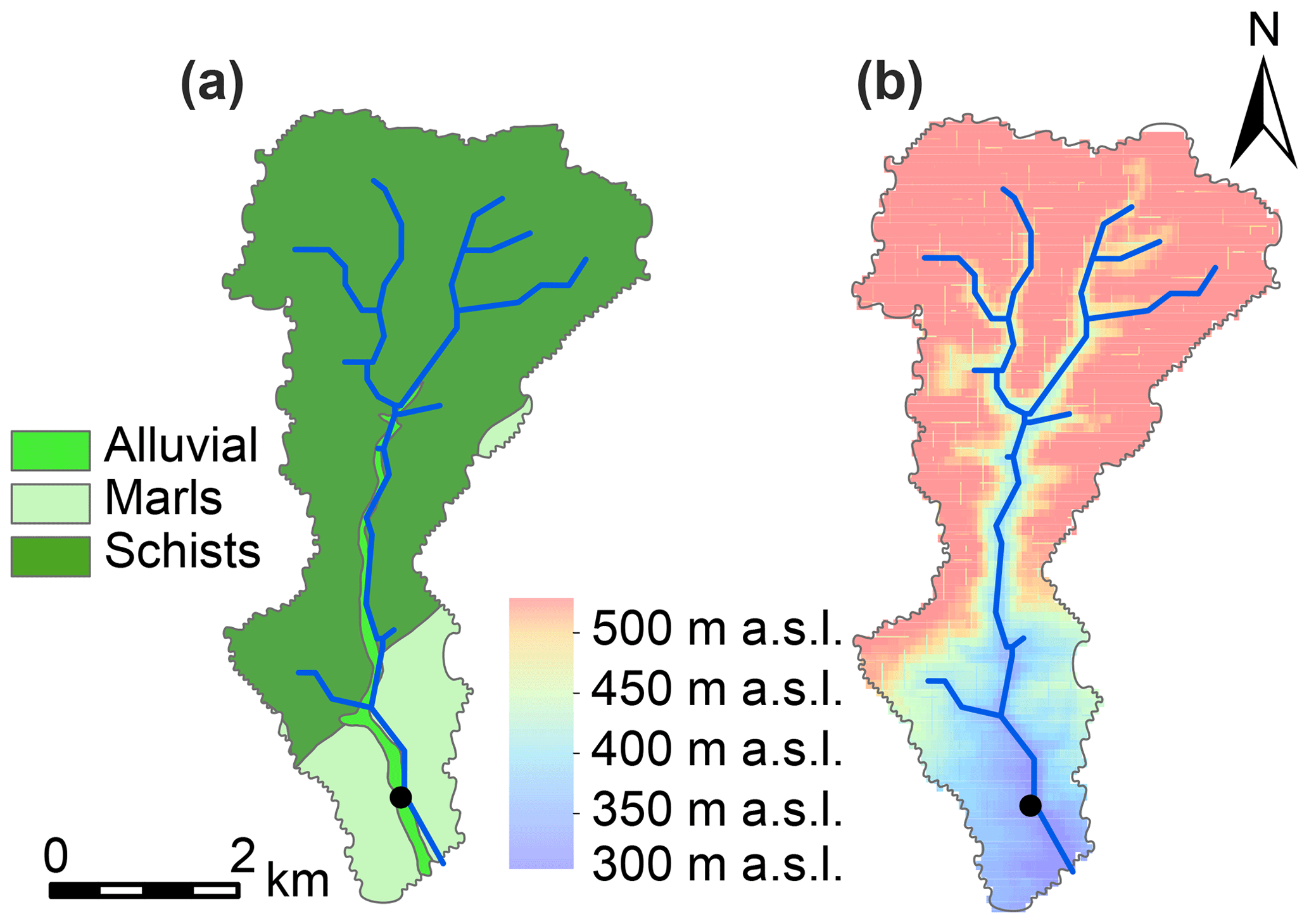
Figure 1Geology (a) and digital elevation model (b) of the Colpach catchment. The black dot marks the sampling location, which is located at the outlet of the catchment (i.e. the Colpach-Haut sub-catchment).
2.2 Experimental set-up
In order to sample drift diatoms and suspended sediment, the sampling location (Fig. 2) was equipped with two automatic water samplers (ISCO 6712 FS) to collect instantaneous stream water samples (1 L). Sampling was triggered by flow conditions and was set up before a rainfall event occurred. During these events, samples were regularly collected every 2 or 3 h. Furthermore, two Phillips samplers were designed as described by Phillips et al. (2000) – except that the diameter of the outlet was 2 mm instead of 4 mm. This was done to increase the settling of sediment in the sampler, as the catchment average suspended sediment concentrations are relatively small. The samplers were attached close to the river bank and downstream of the automatic samplers so that they would not interfere with the samples of the automatic samplers (Fig. 2). The Phillips samplers were placed on site just before the event and were retrieved when the event was completely finished. Concurrently with the placement and removal of the Phillips samplers, we took a manual grab sample (1 L). The Phillips samplers were emptied into 10 L buckets. In addition, turbidity and conductivity were continuously measured in situ at 5 min intervals using a YSI 600OMS optical monitoring system, while water depth was measured with an ISCO 4120 pressure probe logger at a 15 min time step. Discharge at 15 min intervals was estimated using a rating curve between discharge and water level. Upon arrival in the laboratory, all samples were stored at 4 ∘C prior to analysis.
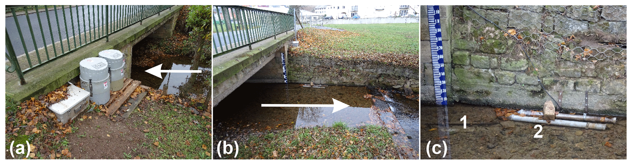
Figure 2Pictures of the experimental set-up at the study location. (a) Automatic samplers installed upstream of the bridge. (b) An overview of the installation of the Phillips samplers downstream of the bridge. The arrow denotes streamflow. (c) A close-up of the turbidity meter (1) and the Phillips samplers (2).
Diatom preparation and identification
After thoroughly shaking the bottles and buckets, a subsample (0.5 L) of each sample was taken for diatom analysis. The subsamples were fixed with 70 % ethanol to prevent a possible population change by cell division and were left aside for at least 1 d to let the diatoms settle down. Diatom slides were prepared for microscopic counts following the European Committee for Standardization (2003). Around 70 % of the supernatant was removed by vacuum aspiration, whereafter samples were cleaned using H2O2 and heated (100 ∘C) for 24 h in a sand bath. The supernatant was removed by aspiration and 1 mL of HCl (37 %) was added. The mixture was allowed to settle for 1 d before the supernatant was removed. Afterwards, three repetitions of rinsing with deionized water, decantation and supernatant removal were carried out. The final suspensions were dried on glass cover slips and mounted on permanent slides using Naphrax. A minimum of 400 valves were counted and identified on each slide (n=103) along random transects using a Leica DMR light microscope with a ×100 oil immersion objective and a magnification of ×1000. Diatom identifications were mainly based on following taxonomic references: Krammer (2000), Lange-Bertalot (2001), Levkov et al. (2016) and Lange-Bertalot et al. (2017).
2.3 Suspended sediment analysis
The suspended sediment concentration (SSC) was determined by filtering a known subsample volume between 200 and 500 mL through 1.2 µm Whatman GF/C glass fibre filters using a Millipore vacuum pump. Prior to filtering, the filters were dried at 105 ∘C and weighed. Afterwards, the samples were dried (105 ∘C) and weighed again. The concentration of suspended sediment was calculated as the difference between these two weights divided by the volume of the filtered sample.
The particle size distribution (PSD) was measured in the laboratory using a portable LISST-200X sensor (Sequoia Scientific, Inc., Bellevue, WA), which is a submersible laser-diffraction-based particle size analyser. Measurements were carried out on suspensions inside a test chamber provided by the manufacturer. Before undertaking the measurements, a background measurement was carried out with Milli-Q water. After the chamber was filled, the water was stirred for a few minutes using a magnetic stirrer to ensure that all bubbles disappeared. If bubbles were still present, they were removed manually from the measuring cell and the windows of the chamber. After carrying the background measurements out, the chamber was filled with a 0.5 L subsample and Milli-Q water was added if the sensor was not fully covered. The magnetic stirrer kept all particles in suspension. Next, a LISST measurement consisting of 120 single measurements was performed in real-time mode using the LISST-SOP200X program. The raw data from each single measurement were then converted to the particle size distribution using the “Random Particle Shape Models” described by Agrawal et al. (2008) and the recorded background scatter. Unfortunately, it was not possible to measure the PSD and SSC in all samples due to the limited water volumes collected.
2.4 Statistical analysis
We performed weighted t tests using the discharge as the weight on the particle size (the 10th, 50th and 90th percentiles), and we compared the distributions using a Kolmogorov–Smirnov test. We used discharge as the weight because a larger volume of water flows through the Phillips sampler during periods of higher discharge and, thus, contributes more to the time-integrated samples. Furthermore, we plotted flow duration curves using the fdc function from the hydroTSM R package (Zambrano-Bigiarini, 2017) in order to check if the events were fully covered by the automated sampling method. We encountered a problem with the field instrumentation during the third event, as the turbidity was exceptionally noisy and the measured concentrations were too high and unrealistic for the site (see Fig. 3). Therefore, we decided to exclude the event from further analysis of the sediment data.
Before carrying out the statistical analysis on the diatom communities, we reduced the species dataset by only retaining taxa with a relative abundance of at least 1 % in a minimum of two samples; the purpose of this was to compare the main patterns in the communities between sampling methods. As the species data contained many zeros, we used a Hellinger transformation on the data and took Euclidean distances using the vegdist function provided by the vegan R package (Oksanen et al., 2019). We then performed non-metric multidimensional scaling (NMDS) analysis. We achieved a stress value below 0.10 which indicates an ideal representation of the data (i.e. the configuration is close to actual dissimilarities) according to Clarke (1993). Afterwards, we compared the position of the centroids in the geometric framework of the NMDS plot using permutational multivariate analysis of variance (PERMANOVA). Differences in treatments were additionally analysed with the betadisper function to check whether these differences were caused by a difference in dispersion (within-group variation) rather than a difference in the mean values of the groups. Furthermore, we used analysis of similarity (ANOSIM) to test if communities significantly differed between the events and sampling methods whilst accounting for repeated measurements, i.e. pseudo-replication (Clarke, 1993). Outcomes were assessed with the Monte Carlo permutation test (perm=9999). Moreover, species relative abundances were compared using similarity analysis (SIMPER) and an unpaired weighted t test or Mann–Whitney U test (sjstats package) with the discharge as weight.
Next, we calculated the diatom biovolume according to the data provided in Rimet and Bouchez (2012) and OMNIDIA (Lecointe et al., 1993) as a measure of the mean cell size. Also, the Shannon–Wiener, Pielou's evenness and specific pollution sensitivity (IPS; Cemagref, 1982) indices were computed and compared for each method and event using an unpaired weighted t test or Mann–Whitney U test. The IPS was chosen from many different diatom-based indices, as this index considers the abundance of each species in the sample, their sensitivity value to organic pollution and their indicator value (i.e. the relative probability of each species to occur in one of five saprobity classes and, in turn, the measure of organic matter present). As the behaviour of diatoms could differ from suspended sediment particles, we assigned an ecological guild to the diatom species following Passy (2007) and Rimet and Bouchez (2012) in order to better understand potential differences in sampling methods. Ecological guilds are defined as a group of species that live in the same environment (i.e. tolerant to similar environmental stressors) but may have adapted differently (Rimet and Bouchez, 2012). All of the aforementioned statistical analyses were performed using the R statistical program (R v. 3.5.0.; http://www.r-project.org/, last access: 21 July 2020).
The first event occurred after an exceptionally dry and warm summer when water levels were very low. Consequently, a maximum catchment discharge of only 0.011 mm h−1 was measured (Fig. 3). Turbidity levels also followed the sudden increase in discharge, reaching 68.5 NTU. Unfortunately, both the automatic and Phillips samplers were not active during the first peak of the event, and this may have influenced our results. The second event occurred a few days later, and the discharge, turbidity and SSC increased substantially during this period. A similar pattern in discharge levels was seen as during the first event (i.e. fast responses to precipitation). This is in strong contrast to the third event, where the small peak in discharge was instead followed by a high, extended peak (i.e. delayed peak). During the third event, we measured the highest catchment discharge (0.44 mm h−1) and turbidity levels. However, the latter showed too much noise; therefore, this event was excluded from the statistical analysis of the sediment data.
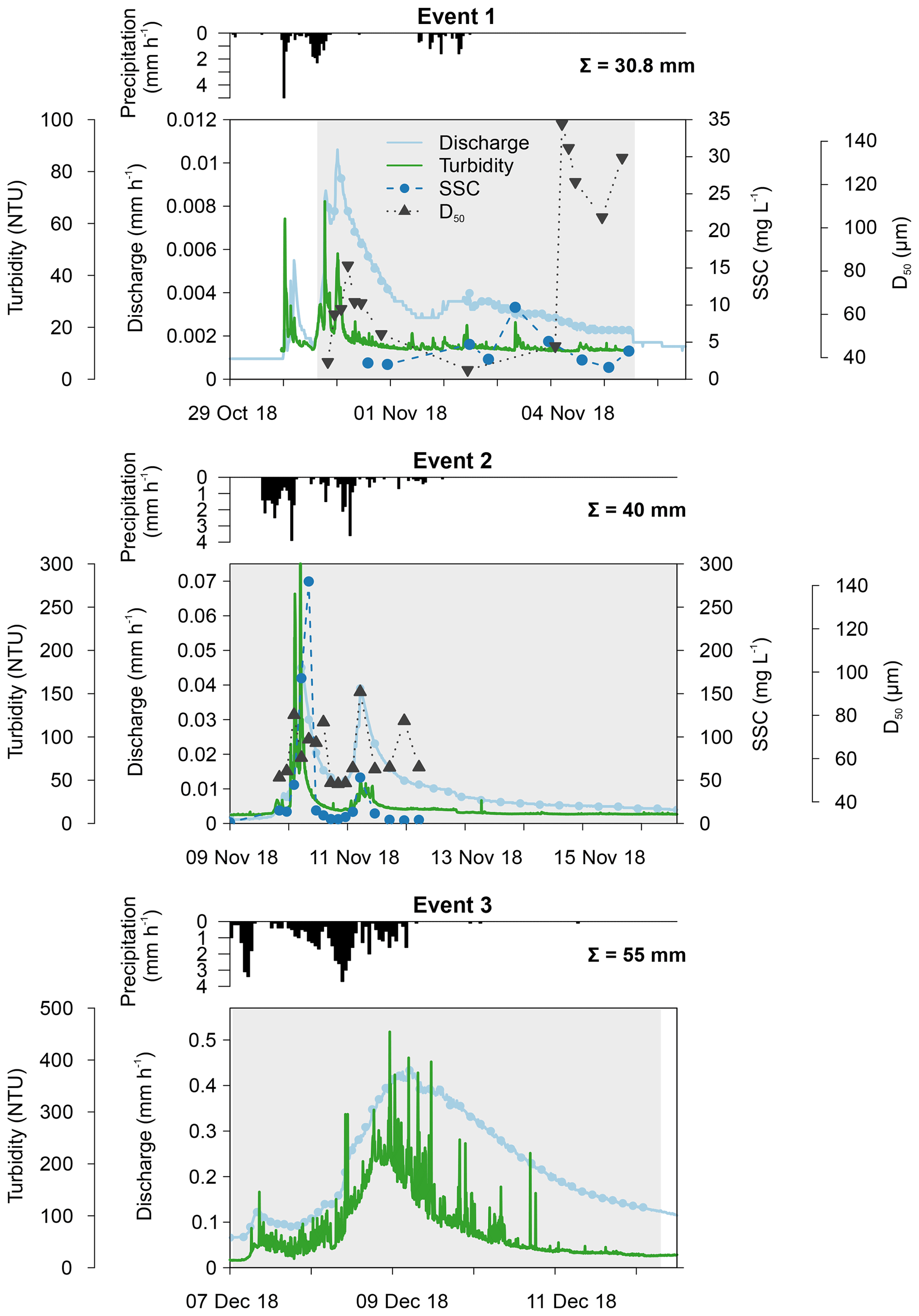
Figure 3Catchment discharge, suspended sediment concentration (SSC), median particle size (D50), turbidity and precipitation for the three events. Discharge and turbidity were measured at 15 min intervals, whereas SSC and D50 were analysed from automatically collected water samples. Total precipitation is given per event. The grey shading represents the period during which the Phillips sampler was in the water.
3.1 Suspended sediment
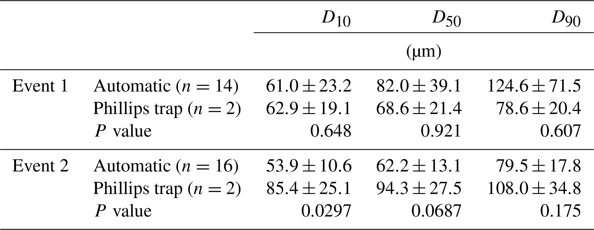
In Figs. 3 and 4, median particle sizes (D50) and PSDs are given for the first two events. In general, the median particle sizes follow the changes in turbidity levels. However, this is not the case for the last five samples taken during the first storm run-off event. These values do not seem correct, as the SSC also shows different behaviour. We do not currently know what caused these high levels, but this effect is also visible in the PSD where a high standard variation is observed after 200 µm. However, we do not observe this second peak in the PSD of the Phillips samples. This difference in the distribution between the two methods was confirmed by the Kolmogorov–Smirnov test (D=0.31, P=0.036), although there was no significant difference for the second event (D=0.25, P=0.21). In addition, we observe that the particle sizes of the Phillips samples are similar to those of the automatic samples (P>0.05), except for the 10th percentile of the second event (, P=0.03) (Table 1). Moreover, we notice that the particle sizes of the time-integrated method substantially increased for the second event, whereas the mean sizes decreased for the automated sampling method. Although, the Phillips sampler has a tendency to undersample smaller particles, it integrates the sediment particle sizes and distributions well on both occasions.

Figure 4Average particle size distribution for the two sampling methods for the first two events. The grey shaded area indicates the standard variation.
Table 1Comparison of the particle size, the 10th (D10), 50th (D50) and 90th (D90) percentiles, between the Phillips sampler and the automatic sampler. Weighted averages and standard deviations are given. P values were derived from weighted t tests or Mann–Whitney U tests.
3.2 Diatom communities
Generally, the flow duration curves show that the three events were well covered by the automatic samplers, because the discharge at the time the automatic sampler collected the samples used for diatom analysis (blue line; Fig. 5) follows a similar pattern to the discharge estimated at 15 min intervals (black line; Fig. 5). Furthermore, the samples are well distributed over the different sampling periods. Both results show us that our sampling was not biased towards certain periods of the events.
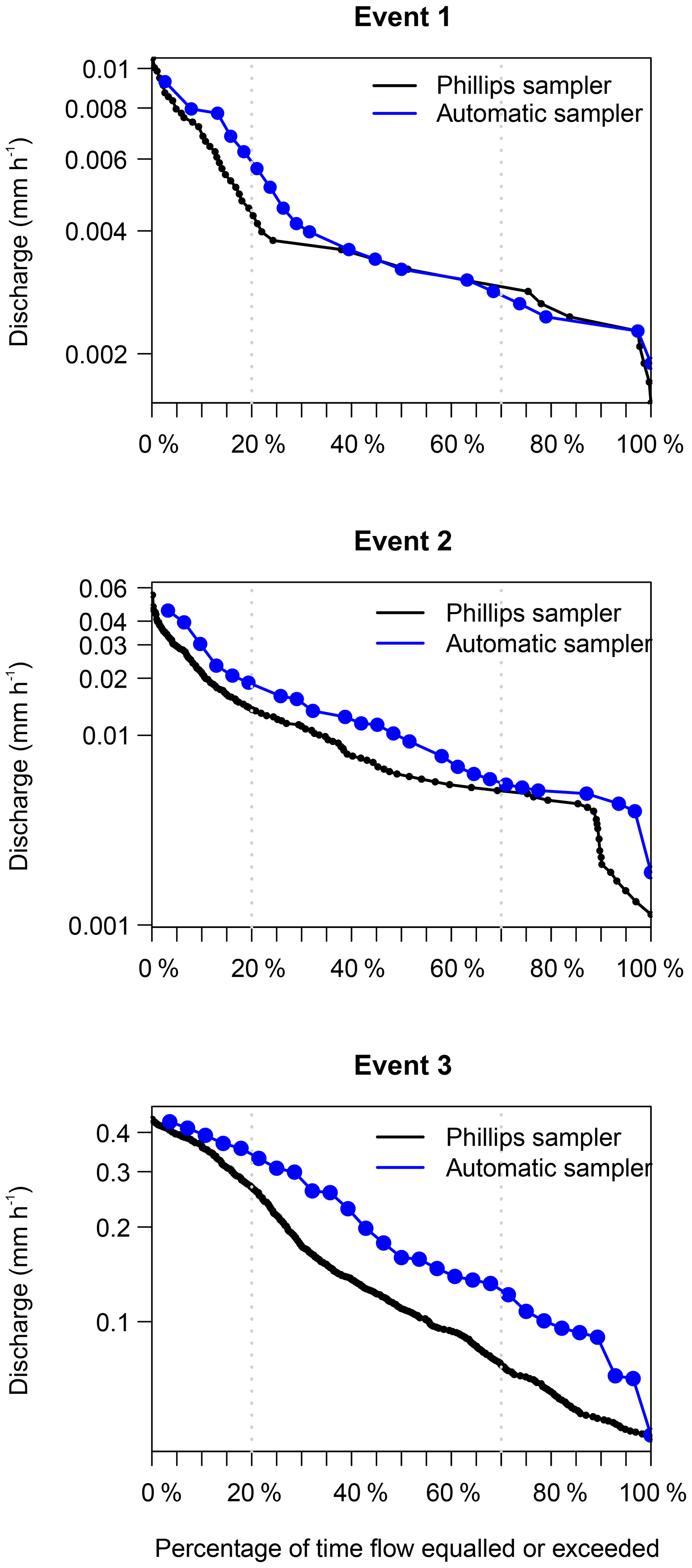
Figure 5Flow duration curves covering the sampling period of the Phillips samplers. The blue line shows the samples taken with an automatic sampler for diatom analysis, and the black line shows the continuous measurements of discharge at 15 min intervals.
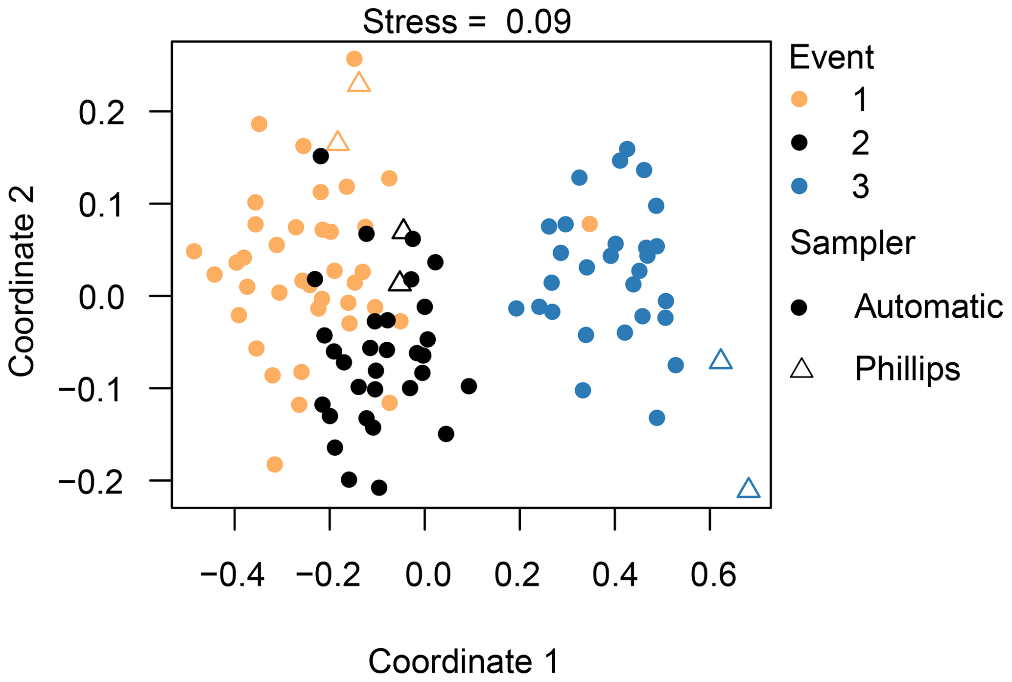
Figure 6Non-metric dimensional scaling (NMDS) analysis of the diatom communities, indicating the different events and sampling methods. Species data underwent a Hellinger transformation and the Euclidean distance was used. A stress value below 0.10 constitutes an ideal representation of the data according to Clarke (1993).
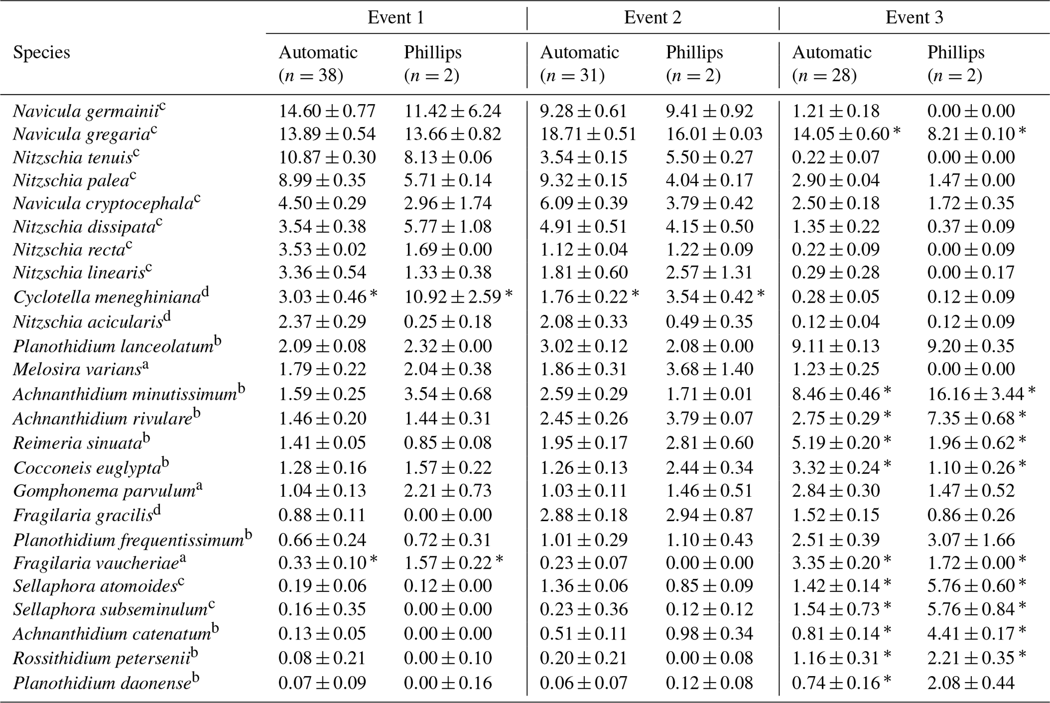
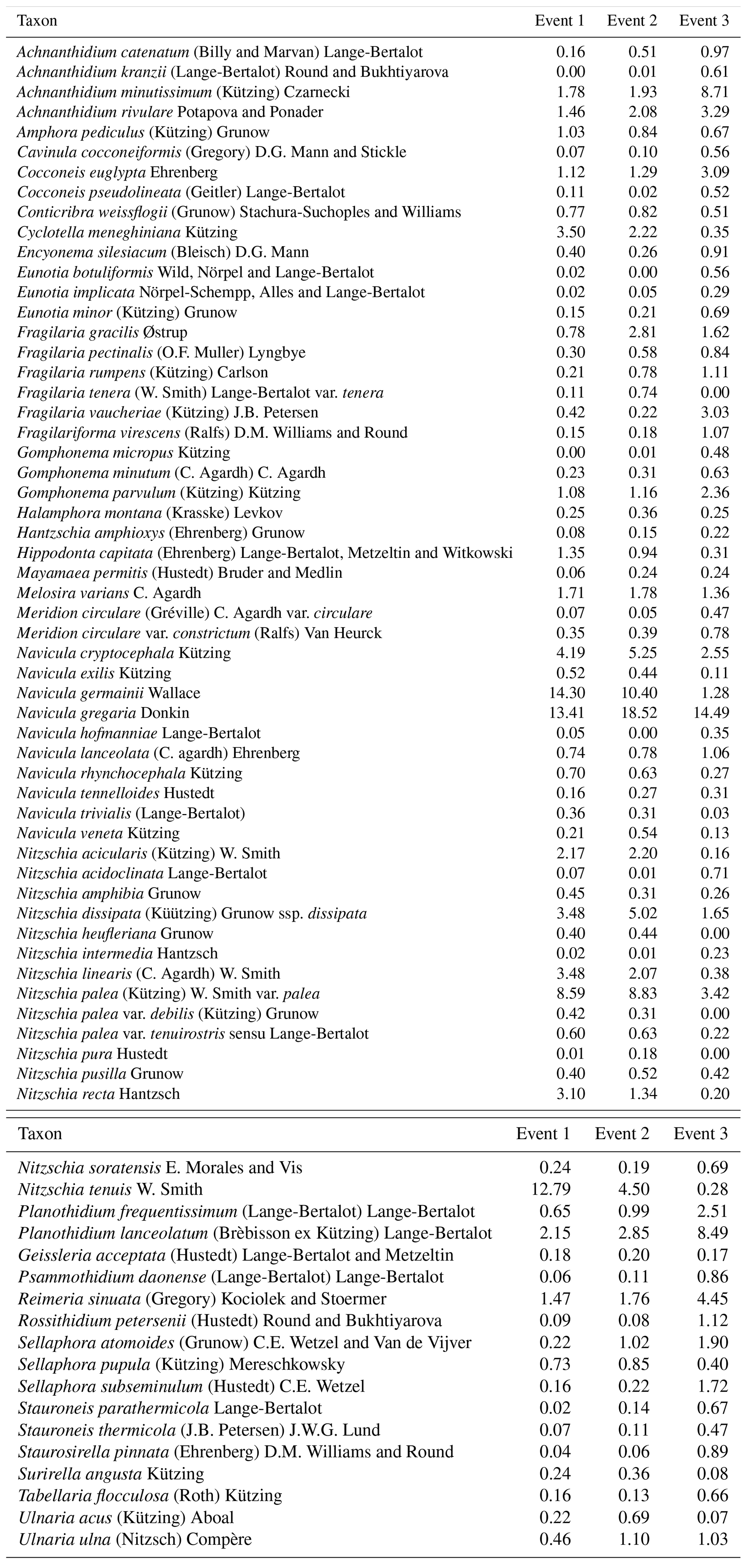
We identified a total of 233 different taxa, including varieties, subspecies and forms, belonging to 65 genera. After using the cut-off criteria, 71 species (94 % of the total valves counted) were retained in the statistical analyses (see Table A1). The most species-rich genera were then Nitzschia, Navicula, Fragilaria and Planothidium, comprising 15, 10, 5 and 4 taxa respectively, whereas Navicula gregaria (15 % of the total valves counted), Navicula germainii (9 %), Nitzschia palea (7.2 %), Nitzschia tenuis (6.5 %) and Planothidium lanceolatum (4.2 %) were the most abundant species. An average species richness per sample of 43±6.8 was observed, with values of 37.9±6.3, 43.7±4.1 and 49±3.9 during the first, second and third events respectively. Terrestrial diatoms were consistently found to react to the precipitation pulses, with the average proportion of terrestrial diatoms in the water samples increasing to a maximum of 6.6 % (event 1), 8.4 % (event 2) and 9.7 % (event 3) during periods of high discharge (see Fig. A1 in Appendix).
Table 2Most abundant diatom species for the whole study campaign. The weighted averages (in percent) and standard error of the relative abundances are given. An ”*” indicates that the species relative abundance is significantly different between the two sampling methods for that event.
The ecological guilds are as follows: a high profile; b low profile; c motile; d planktonic.
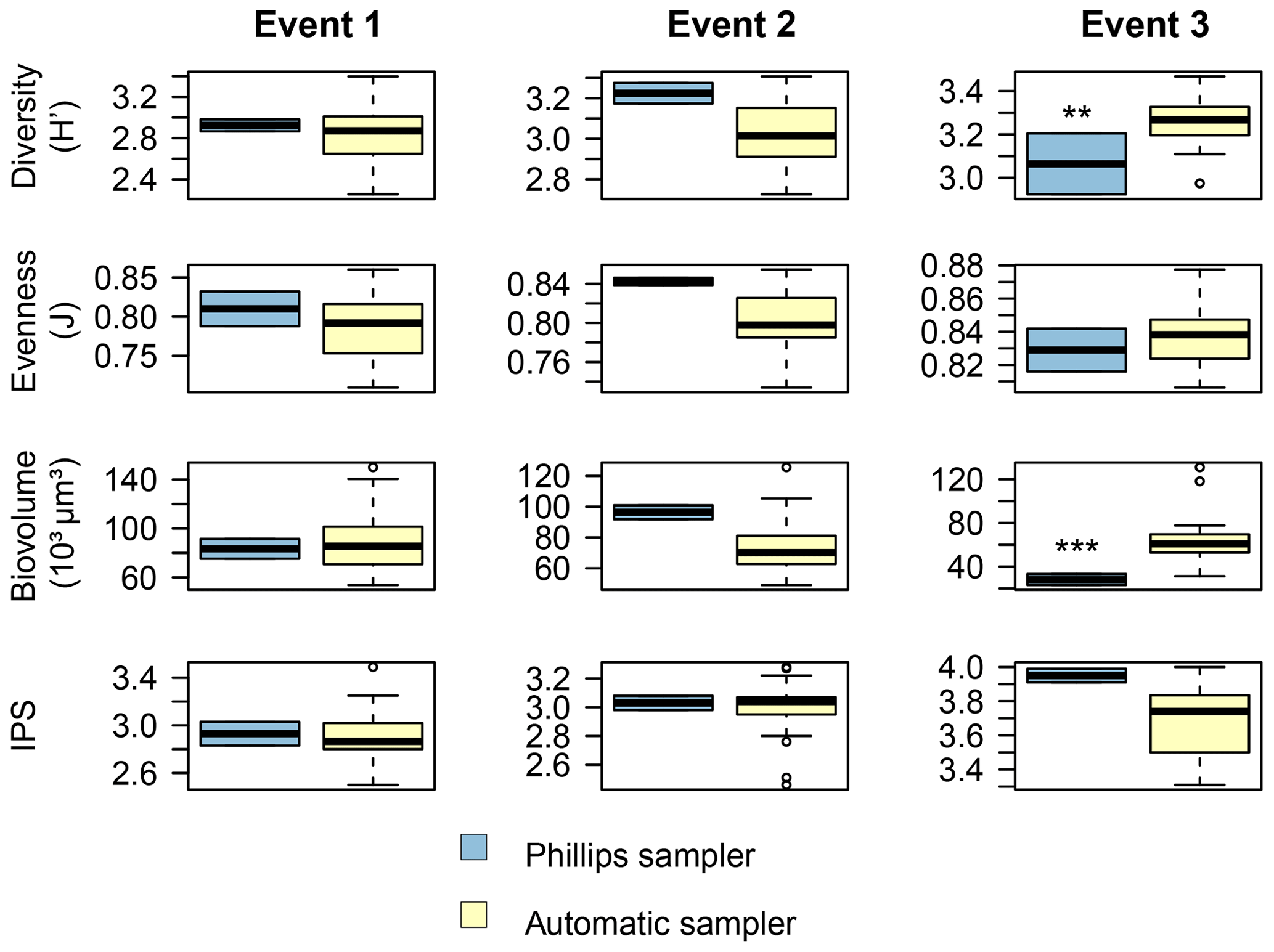
Figure 7Comparison of the diatom community data between the two sampling methods for each event. The Shannon–Wiener index (H′) generally ranges between 1.5 (low diversity) and 3.5 (high diversity). Pielou's evenness (J) ranges between 0 (low evenness) and 1 (high evenness). The specific pollution sensitivity index (IPS) ranges between 1 (poor water quality) and 5 (high quality). Calculations were based on relative abundance data. P<0.01, P<0.001.
Based on the NMDS analysis, we are able to separate the three different events from each other; in particular, the diatom communities taken during the third event are very different from the other two events (Fig. 6). Our PERMANOVA analysis confirmed this observation (F=70.5, P=0.001). Concerning the different sampling methods, we observe that the Phillips samples from the third event are significantly different from most of the automatic samples from that event (F=4.1, P=0.001). Likewise, the time-integrated samples of the second event are quite distinct from each other (F=2.3, P=0.02), whereas the Phillips samples of event 1 are not really distinguishable from each other or from the automatic samples. As the sampling methods showed differences for events 2 and 3, we checked whether these differences may have been caused by a different within-group variation (dispersion) instead of different mean values of the groups. The analysis eventually gave no significant difference (P=0.114), indicating that there was no significant dispersion effect. Overall, the NMDS and PERMANOVA analysis grouped the diatom communities relatively well per event with some time-integrated samples being differentiated from the automatic samples.
Overall, the ANOSIM, species relative abundances (Table 2) and their derived indices (Fig. 7) all seemed to indicate similar results to the NMDS. ANOSIM enabled the detection and split of the communities based on the different events (global R=0.6433, P=0.0001). Moreover, there was also a significant difference between the community composition of the automatic sampler and the Phillips sampler for the third event (R=0.804, P=0.002), whereas the communities taken during the other two events could not be separated from each other (R=0.1713, P=0.08). A similar outcome to previous analyses is seen when we compare the abundances of the most abundant diatom species with each other. Aside from Navicula gregaria and Navicula cryptocephala, which are dominant throughout the entire study, the abundance of the other dominant taxa differ substantially between the first, second and the third events. For instance, Navicula germainii, Nitzschia tenuis and Cyclotella meneghiniana only occur sparingly in the third event, whereas we observe the inverse for Planothidium lanceolatum, Sellaphora subseminulum and Achnanthidium minutissimum. Interestingly, this follows a shift in ecological guilds: from an assemblage containing more motile species (i.e. unattached free-living species immersed on the sediment matrix surrounded by exopolysaccharides) to more colonial and strongly attached taxa. Regarding the sampling methods, dominant taxa such as N. germainii, N. gregaria, N. tenuis and Nitzschia palea vary little during the first two events, except for C. meneghiniana and to a lesser extent Fragilaria vaucheriae which both occur significantly more in the samples from the Phillips sampler. In contrast to those events, the abundances of N. gregaria, Achnanthidium rivulare, A. minutissimum, Reimeria sinuata, Sellaphora atomoides, F. vaucheriae and S. subseminulum are all very different between the methods for the last event. Of these two communities, the one collected with the automatic samplers more appropriately resembles the communities of events 1 and 2. Concerning the indices, the Shannon–Wiener, species evenness and IPS do not show any significant difference between the methods for the first two events (P>0.05), and only a higher diversity in the automatic samplers is noted for the third event (t=2.76, df=28, P=0.01). Moreover, the overall diatom size was higher in the automatic samples of the third event compared with the time-integrated samples (χ2=7.76, df=28, P<0.0001), whereas it was not significantly different for the first two events. Despite the fact that indices do not differ for the second event, we notice that the diversity, evenness and biovolume tend to have higher values for the Phillips samplers. The results of our analyses indicate that the Phillips sampler could possibly be a valid tool for collecting a time-integrated diatom community representative of the entire sampling period.
4.1 Evaluation of the events and sampling methods
The purpose of this study was to test if the Phillips sampler could be used to collect a time-integrated diatom assemblage as an alternative to automated sampling methods. To evaluate the Phillips sampler, three storm run-off events were simultaneously sampled with automatic samplers and analysed. The events were thoroughly covered, as shown in the flow duration curves. From these three events, two different types of hydrographs were generated, and NMDS analysis showed that the events could be separated based on the diatom species composition. Even though we only sampled at one location over a relatively short period (30 October–12 December), we were able to observe a noteworthy amount of variation among events and communities.
Furthermore, previous results from Klaus et al. (2015) and Pfister et al. (2017) confirm that we did sample representative communities of the stream. Like us, they carried out event-based sampling in the Colpach catchment at the same time of year (December). The time of year is important, as diatoms exhibit seasonal succession; thus, the species composition could change significantly during the year (Wetzel, 2001; Wu et al., 2016). Klaus et al. (2015) analysed 28 samples in which they found 221 different species, while we also observed 231 taxa. Likewise, Klaus et al. (2015) found that the percentage of terrestrial diatoms in the samples increased to 8.9 % during the first precipitation pulse at a discharge of around 0.18 mm h−1, which is also the proportion that we found. Of the 15 most abundant species in their study, 12 were also present in our study and 8 of these 12 were abundant, including N. gregaria, P. lanceolatum, N. cryptocephala and N. linearis. Similarly, of the 15 dominant species in Pfister et al. (2017), 11 were present in this study and 6 of these 11 were dominant, including N. gregaria, N. palea, A. minutissimum and P. lanceolatum. Our research also confirms the observation of Martínez-Carreras et al. (2015), who found that the relative abundance of terrestrial diatoms increased with higher discharge. Unfortunately, as we encountered too much noise in the turbidity and sediment analysis of the third event, is it difficult to draw robust conclusions from that event. The reasons for this noise are still unknown and may be linked to a local accumulation of sediment and fine material on and around the sampling tubing of the automatic samplers and inadequate cleaning of the turbidity sensor. However, aside from this noise, the results indicate that (1) sampling was generally carried out properly, (2) there was some variation between and during the events, and (3) samples were representative of the site.
4.2 The potential for the Phillips sampler to collect drift diatoms
Several statistical analyses were executed on sediment and diatom data to verify if the Phillips sampler could be a useful tool for sampling drift diatoms. As shown here (and previously by several other studies), the Phillips sampler gives reasonably good results concerning particle sizes and particle size distributions when compared to automated sampling methods (Phillips et al., 2000; Walling, 2005; Perks et al., 2014; Smith and Owens, 2014). The oversampling of bigger sediment particles, as often mentioned in previous studies, did occur, but this effect was rather limited in this research. Despite differences in the behaviour of diatoms and suspended sediment particles (e.g. smaller mass density, formation of aggregates and circadian diurnal activity rhythm), there was only one time-integrated sample that deviated from the other time-integrated and automatic samples for the first two events. Besides this one sample, no significant differences in the communities and their derivatives, such as biovolume and diversity, were observed between the two sampling methods for the first two events, although communities tend to be bigger and more diverse for the Phillips samples for the second event. However, time-integrated communities sampled during the third event differed from the assemblages collected with the automatic sampler. This is probably due to the same reason as the excessive noise in the sediment data. As these samples were collected using automated sampling, one could argue that the Phillips sampler should give the better results of the two methods. This is, however, not reflected in the diatom communities, because they actually differed more from the communities sampled in the previous events. Conversely, the stream did show different behaviour, higher discharge and water level, compared with the other events, and this likely led to the activation, detachment and transportation of species that show different behaviour or species that belong to a different ecological guild, e.g. more strongly attached species (see examples in Round et al., 1990; Jewson et al., 2006; Rimet and Bouchez, 2012). Indeed, highly motile and planktonic species such as Navicula sp. and Nitzschia sp. were replaced by colonial and/or attached species (e.g. Achnanthidium sp. and Planothidium sp.), and this shift was more pronounced in the Phillips sampler. Thus, the Phillips sampler seems to be able to sample a representative diatom community for a storm run-off event, although we were not able to check whether the underestimation of certain species occurred during the third event.
4.3 Potential way forward
Today, different research avenues can be followed in the exploration of drift diatom sampling methods for hydrological tracing. Here, the Phillips sampler was successfully applied, although our work was restricted to a single location. Therefore, future studies should aim to test the sampler in other settings that have different hydrological behaviour and diatom communities. It would be interesting to investigate if studies would then be able to confirm our results and, specifically, provide information on the efficiency of the Phillips sampler at higher discharges, which is still not clear from our study. Furthermore, future research should not be limited to the Phillips sampler alone; other passive samplers such as the pumped active suspended sediment (PASS) sampler designed by Doriean et al. (2019) and the bidirectional time-integrated mass-flux sampler (TIMS) developed by Elliott et al. (2017) should also be able to collect representative diatom communities. The operating principle of both of these samplers is the same as that of the Phillips sampler with the difference being that the PASS works at a constant, predefined flow rate, enabling the measurements of time-weighted average SSC and PSD, whereas the bidirectional TIMS was developed for estuaries and has an L-shaped outlet preventing inflow from the other direction. Another possible avenue would be the investigation of the minimum number of point samples that is needed and the periods during which the samples should be taken (e.g. one at peak discharge, during rising and falling limb) to get a community representing the entire event. Importantly, the diurnal circadian rhythm of benthic diatoms should also be taken into account (Müller-Haeckel, 1973; Müller-Haeckel and Håkansson, 1978). Eventually, this information could then significantly reduce the number of samples analysed. Furthermore, molecular techniques (i.e. DNA metabarcoding and high-throughput sequencing) are developing quickly in diatom research, and as these techniques are faster and less expensive than microscopical examinations, they could also open the door to higher-frequency sampling (Vasselon et al., 2017; Rivera et al., 2020). Thus, this research has unlocked new possibilities for collecting drift diatoms which could pave the way for the better use of diatoms in hydrological tracing.
Increased amounts of suspended sediments due to anthropogenic factors can have significant negative impacts on water quality and aquatic biota. It can also reduce primary production through a reduction in light penetration and can act as an important vector for the transfer of nutrients and metals in fluvial systems (Bowes et al., 2003; Ballantine et al., 2008; Bilotta and Brazier, 2008). Therefore, it is important to identify sediment sources and their relative contribution to the overall sediment load in order to establish their effect on the ecological functioning of the system so that remedial measures can be taken. A way to investigate this is with sediment fingerprinting. Regarding this technique, several tracers (e.g. mineralogy, nitrogen and carbon stable isotopes) are used to serve as sediment fingerprints (Haddadchi et al., 2013). As (drift) diatoms are often associated with those particles, they could provide additional information on sediment quality, its sources and its transport (Jewson et al., 2006; Jones et al., 2012). More interestingly, they could even be sampled and analysed with the suspended sediment in order to determine potential (sediment) sources and their relative contribution in a catchment (Pfister et al., 2017). Furthermore, the use of a time-integrated sampler also enables us to collect a phytoplankton community, even at different depths (McDonald et al., 2010). Generally, in water quality assessment, phytoplankton is sampled with grab samples (Soylu and Gönülol, 2003; Abonyi et al., 2012). However, the composition of planktonic diatoms is quite variable in time and changes occur relatively quickly in comparison to benthic communities (Round et al., 1990). Therefore, it would be interesting to test if a time-integrated suspended sediment sampler would also give a representative phytoplankton community for a certain period of time. Hence, the use of a time-integrated mass-flux sampler could not only assist sediment fingerprinting but could potentially also improve the analysis of water quality.
Here, we investigated if the Phillips sampler, a time-integrated mass-flux sampler, was able to sample representative diatom communities during a storm run-off event. This was done by comparing the suspended sediment concentrations, particle size distributions and drift diatom assemblages with point samples collected by automatic samplers. Most of our results indicate that the Phillips sampler sampled representative samples during two storm run-off events, although significantly different communities were collected during the third event. However, sediment data from this event, which was sampled with automatic samplers, showed a large amount of noise, meaning that we could not verify if the Phillips sampler sampled representative communities or not. Nevertheless, we believe that this sampler could not only be applied in hydrological tracing using terrestrial diatoms but may also be a useful tool in water quality assessment.
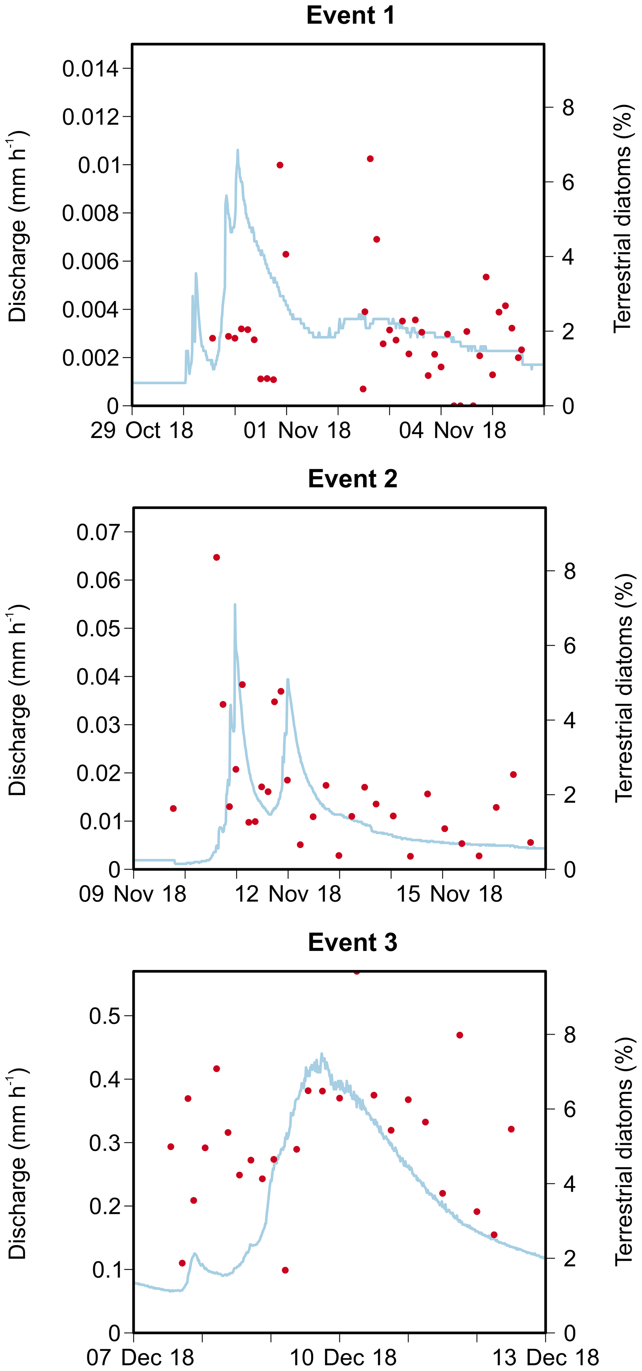
Figure A1Discharge and relative abundances of terrestrial diatoms in the community for the three storm run-off events.
Table A1Species list with species relative abundances (%) per event. The list only includes taxa with a relative abundance of at least 1 % in a minimum of two samples.
The data underlying this research can be found at https://doi.org/10.17632/hgbf5bpwkh.1 (Foets et al., 2020c).
JF, CEW, AJT, NMC and LP designed and directed the study. JFI planned and carried out the field work. NMC carried out the analysis of the sediment data. JF prepared the diatom slides and carried out diatom identifications. JF, CEW, NMC, LP and AJT discussed and interpreted the results. JF prepared the paper with contributions from all co-authors.
The authors declare that there is no conflict of interest.
The authors thank Francis Burdon and the anonymous reviewer for their constructive comments that improved the paper.
This research has been supported by the Luxembourg National Research Fund (FNR; grant no. PRIDE15/10623093/HYDRO-CSI).
This paper was edited by Christian Stamm and reviewed by Francis Burdon and one anonymous referee.
Abonyi, A., Leitão, M., Lançon, A. M., and Padisák, J.: Phytoplankton functional groups as indicators of human impacts along the River Loire (France), Hydrobiologia, 698, 233–249, https://doi.org/10.1007/s10750-012-1130-0, 2012. a
Agrawal, Y. C., Whitmire, A., Mikkelsen, O. A., and Pottsmith, H. C.: Light scattering by random shaped particles and consequences on measuring suspended sediments by laser diffraction, J. Geophys. Res., 113, C04023, https://doi.org/10.1029/2007JC004403, 2008. a
Antonelli, M., Wetzel, C. E., Ector, L., Teuling, A. J., and Pfister, L.: On the potential for terrestrial diatom communities and diatom indices to identify anthropic disturbance in soils, Ecol. Indic., 75, 73–81, https://doi.org/10.1016/j.ecolind.2016.12.003, 2017. a
Ballantine, D. J., Walling, D. E., Collins, A. L., and Leeks, G. J.: The phosphorus content of fluvial suspended sediment in three lowland groundwater-dominated catchments, J. Hydrol., 357, 140–151, https://doi.org/10.1016/j.jhydrol.2008.05.011, 2008. a
Bilotta, G. S. and Brazier, R. E.: Understanding the influence of suspended solids on water quality and aquatic biota, Water Res., 42, 2849–2861, https://doi.org/10.1016/j.watres.2008.03.018, 2008. a
Bowes, M. J., House, W. A., and Hodgkinson, R. A.: Phosphorus dynamics along a river continuum, Sci. Total Environ., 313, 199–212, https://doi.org/10.1016/S0048-9697(03)00260-2, 2003. a
Burns, D. A.: Stormflow-hydrograph separation based on isotopes: the thrill is gone – what's next?, Hydrol. Process., 16, 1515–1517, https://doi.org/10.1002/hyp.5008, 2002. a
Cemagref: Etude des méthodes biologiques d'appréciation quantitative de laqualité des eaux, Tech. rep. No. 66/45396, 218 pp., Cemagref, Division Qualité des Eaux, Lyon, 1982. a
Clarke, K. R.: Non-parametric multivariate analyses of changes in community structure, Aust. J. Ecol., 18, 117–143, https://doi.org/10.1111/j.1442-9993.1993.tb00438.x, 1993. a, b, c
Doriean, N. J., Teasdale, P. R., Welsh, D. T., Brooks, A. P., and Bennett, W. W.: Evaluation of a simple, inexpensive, in situ sampler for measuring time-weighted average concentrations of suspended sediment in rivers and streams, Hydrol. Process., 33, 678–686, https://doi.org/10.1002/hyp.13353, 2019. a
Droppo, I. G.: Rethinking what constitutes suspended sediment, Hydrol. Process., 15, 1551–1564, https://doi.org/10.1002/hyp.228, 2001. a
Elliott, E. A., Monbureau, E., Walters, G. W., Elliott, M. A., McKee, B. A., and Rodriguez, A. B.: A novel method for sampling the suspended sediment load in the tidal environment using bi-directional time-integrated mass-flux sediment (TIMS) samplers, Estuar. Coast. Shelf S., 199, 14–24, https://doi.org/10.1016/j.ecss.2017.08.029, 2017. a
Elsenbeer, H., Lorieri, D., and Bonell, M.: Mixing model approaches to estimate storm flow sources in an overland flow-dominated tropical rain forest catchment, Water Resour. Res., 31, 2267–2278, https://doi.org/10.1029/95WR01651, 1995. a
European Committee for Standardization: Water quality-Guidance standard for the routine sampling and pretreatment of benthic diatoms from rivers, EN 13946, European Committee for Standardization, Brussels, 2003. a
Fenicia, F., Wrede, S., Kavetski, D., Pfister, L., Hoffmann, L., Savenije, H. H. G., and McDonnell, J. J.: Assessing the impact of mixing assumptions on the estimation of streamwater mean residence time, Hydrol. Process., 24, 1730–1741, https://doi.org/10.1002/hyp.7595, 2010. a
Foets, J., Wetzel, C. E., Teuling, A. J., and Pfister, L.: Temporal and spatial variability of terrestrial diatoms at the catchment scale: controls on communities, PeerJ, 8, e8296, https://doi.org/10.7717/peerj.8296, 2020a. a, b
Foets, J., Wetzel, C. E., Teuling, A. J., and Pfister, L.: Temporal and spatial variability of terrestrial diatoms at the catchment scale: controls on productivity and comparison with other soil algae, PeerJ, 8, e9198, https://doi.org/10.7717/peerj.9198, 2020b. a
Foets, J., Martínez-Carreras, N., Iffly, J., and Pfister, L.: A time-integrated sediment trap to sample diatoms for hydrological tracing, Mendeley Data, V1, https://doi.org/10.17632/hgbf5bpwkh.1, 2020c. a
Gerbersdorf, S. U., Jancke, T., Westrich, B., and Paterson, D. M.: Microbial stabilization of riverine sediments by extracellular polymeric substances, Geobiology, 6, 57–69, https://doi.org/10.1111/j.1472-4669.2007.00120.x, 2008. a
Haddadchi, A., Ryder, D. S., Evrard, O., and Olley, J.: Sediment fingerprinting in fluvial systems: Review of tracers, sediment sources and mixing models, Int. J. Sediment Res., 28, 560–578, https://doi.org/10.1016/S1001-6279(14)60013-5, 2013. a
Hooper, R. P., Christophersen, N., and Peters, N. E.: Modelling streamwater chemistry as a mixture of soilwater end-members – An application to the Panola Mountain catchment, Georgia, U.S.A., J. Hydrol., 116, 321–343, https://doi.org/10.1016/0022-1694(90)90131-G, 1990. a
Hutchinson, G.: Introduction to lake biology and the limnoplankton, in: A treatise Limnol., Wiley, New York, 2nd edn., 1115 pp., 1967. a
Jewson, D. H., Lowry, S. F., and Bowen, R.: Co-existence and survival of diatoms on sand grains, Eur. J. Phycol., 41, 131–146, https://doi.org/10.1080/09670260600652903, 2006. a, b
Jones, J. I., Duerdoth, C. P., Collins, A. L., Naden, P. S., and Sear, D. A.: Interactions between diatoms and fine sediment, Hydrol. Process., 28, 1226–1237, https://doi.org/10.1002/hyp.9671, 2012. a, b
Juilleret, J., Iffly, J. F., Pfister, L., and Hissler, C.: Remarkable Pleistocene periglacial slope deposits in Luxembourg (Oesling): pedological implication and geosite potential, Bulletin de la Société des naturalistes luxembourgeois, 112, 125–130, 2011. a
Keck, F., Vasselon, V., Rimet, F., Bouchez, A., and Kahlert, M.: Boosting DNA metabarcoding for biomonitoring with phylogenetic estimation of operational taxonomic units’ ecological profiles, Mol. Ecol. Resour., 18, 1299–1309, https://doi.org/10.1111/1755-0998.12919, 2018. a
Klaus, J., Wetzel, C. E., Martínez-Carreras, N., Ector, L., and Pfister, L.: A tracer to bridge the scales: on the value of diatoms for tracing fast flow path connectivity from headwaters to meso-scale catchments, Hydrol. Process., 29, 5275–5289, https://doi.org/10.1002/hyp.10628, 2015. a, b, c, d, e
Krammer, K.: The genus Pinnularia, in: Diatoms of Europe: Diatoms of the European inland waters and comparable habitats, edited by: Lange-Bertalot, H.,ARG Gantner Verlag KG, Ruggell, 1, 703 pp., 2000. a
Lange-Bertalot, H.: Navicula sensu stricto; 10 genera separated from Navicula sensu lato Frustulia, in: Diatoms of Europe: Diatoms of the European inland waters and comparable habitats, edited by: Lange-Bertalot, H., Gantner Verlag KG, Ruggell, 2, 526 pp., 2001. a
Lange-Bertalot, H., Hofmann, G., Werum, M., Cantonati, M., and Kelly, M. G.: Freshwater benthic diatoms of Central Europe: Over 800 common species used in ecological assessment, Koeltz Botanical Books Schmitten-Oberreifenberg, Germany, 2017. a
Laubel, A., Kronvang, B., Fjorback, C., and Larsen, S. E.: Time-integrated suspended sediment sampling from a small lowland stream, SIL Proceedings, 1922–2010, 28, 1420–1424, https://doi.org/10.1080/03680770.2001.11902689, 2002. a, b
Lecointe, C., Coste, M., and Prygiel, J.: “Omnidia”: software for taxonomy, calculation of diatom indices and inventories management, Hydrobiologia, 269, 509–513, https://doi.org/10.1007/BF00028048, 1993. a
Levkov, Z., Mitic-Kopanja, D., and Reichardt, E.: The diatom genus Gomphonema from the Republic of Macedonia, in: Diatoms of Europe: Diatoms of the European inland waters and comparable habitats, edited by: Lange-Bertalot, H., Koeltz Scientific Books, Königstein, 8, 552 pp., 2016. a
Loritz, R., Hassler, S. K., Jackisch, C., Allroggen, N., van Schaik, L., Wienhöfer, J., and Zehe, E.: Picturing and modeling catchments by representative hillslopes, Hydrol. Earth Syst. Sci., 21, 1225–1249, https://doi.org/10.5194/hess-21-1225-2017, 2017. a
Lund, J. W. G.: Observations on soil algae. I. The ecology, size and taxonomy of British soil diatoms, New Phytol., 44, 196–219, 1945. a
Martínez-Carreras, N., Krein, A., Gallart, F., Iffly, J. F., Pfister, L., Hoffmann, L., and Owens, P. N.: Assessment of different colour parameters for discriminating potential suspended sediment sources and provenance: A multi-scale study in Luxembourg, Geomorphology, 118, 118–129, https://doi.org/10.1016/j.geomorph.2009.12.013, 2010. a, b
Martínez-Carreras, N., Krein, A., Gallart, F., Iffly, J. F., Hissler, C., Pfister, L., Hoffmann, L., and Owens, P. N.: The influence of sediment sources and hydrologic events on the nutrient and metal content of fine-grained sediments (Attert River basin, Luxembourg), Water Air Soil Poll., 223, 5685–5705, https://doi.org/10.1007/s11270-012-1307-1, 2012. a, b
Martínez-Carreras, N., Wetzel, C. E., Frentress, J., Ector, L., McDonnell, J. J., Hoffmann, L., and Pfister, L.: Hydrological connectivity inferred from diatom transport through the riparian-stream system, Hydrol. Earth Syst. Sci., 19, 3133–3151, https://doi.org/10.5194/hess-19-3133-2015, 2015. a, b
McDonald, D. M., Lamoureux, S. F., and Warburton, J.: Assessment of a time-integrated fluvial suspended sediment sampler in a high arctic setting, Geogr. Ann. A, 92, 225–235, https://doi.org/10.1111/j.1468-0459.2010.00391.x, 2010. a, b
McDonnell, J. J., Bonell, M., Stewart, M. K., and Pearce, A. J.: Deuterium variations in storm rainfall: Implications for stream hydrograph separation, Water Resour. Res., 26, 455–458, https://doi.org/10.1029/WR026i003p00455, 1990. a
Müller-Haeckel, A. and Håkansson, H.: The diatom flora of a small stream near Abisko (Swedish Lapland) and its annual periodicity, judged by drift and colonisation, Archiv für Hydrobiologie., 84, 199–217, 1978. a, b
Müller-Haeckel, A.: Different patterns of synchronization in diurnal and nocturnal drifting algae in the subarctic summer, Aquil. Ser. Zool., 14, 19–22, 1973. a, b
Oksanen, J., Blanchet, F. G., Friendly, M., Kindt, R., Legendre, P., McGinn, D., Minchin, P. R., O'Hara, R., Simpson, G. L., Solymos, P., Stevens, M. H. H., Szoecs, E., and Wagner, H.: Vegan: community ecology package. R package version 2.5-5, available at: https://cran.r-project.org/package=vegan (last access: 21 July 2020), 2019. a
Passy, S. I.: Diatom ecological guilds display distinct and predictable behavior along nutrient and disturbance gradients in running waters, Aquat. Bot., 86, 171–178, https://doi.org/10.1016/j.aquabot.2006.09.018, 2007. a
Perks, M. T., Warburton, J., and Bracken, L.: Critical assessment and validation of a time-integrating fluvial suspended sediment sampler, Hydrol. Process., 28, 4795–4807, https://doi.org/10.1002/hyp.9985, 2014. a, b
Pfister, L., McDonnell, J. J., Wrede, S., Hlúbiková, D., Matgen, P., Fenicia, F., Ector, L., and Hoffmann, L.: The rivers are alive: on the potential for diatoms as a tracer of water source and hydrological connectivity, Hydrol. Process., 23, 2841–2845, https://doi.org/10.1002/hyp.7426, 2009. a, b
Pfister, L., Wetzel, C. E., Martínez-Carreras, N., Iffly, J. F., Klaus, J., Holko, L., and McDonnell, J. J.: Examination of aerial diatom flushing across watersheds in Luxembourg, Oregon and Slovakia for tracing episodic hydrological connectivity, J. Hydrol. Hydromech., 63, 235–245, https://doi.org/10.1515/johh-2015-0031, 2015. a
Pfister, L., Wetzel, C. E., Klaus, J., Martínez‐Carreras, N., Antonelli, M., Teuling, A. J., and McDonnell, J. J.: Terrestrial diatoms as tracers in catchment hydrology: a review, WIREs Water, 4, e1241, https://doi.org/10.1002/wat2.1241, 2017. a, b, c, d
Phillips, J. M., Russell, M. A., and Walling, D. E.: Time-integrated sampling of fluvial suspended sediment: A simple methodology for small catchments, Hydrol. Process., 14, 2589–2602, https://doi.org/10.1002/1099-1085(20001015)14:14<2589::AID-HYP94>3.0.CO;2-D, 2000. a, b, c, d, e
Rimet, F. and Bouchez, A.: Life-forms, cell-sizes and ecological guilds of diatoms in European rivers, Knowl. Manag. Aquat. Ec., 406, 1–12, https://doi.org/10.1051/kmae/2012018, 2012. a, b, c, d
Rivera, S. F., Vasselon, V., Bouchez, A., and Rimet, F.: Diatom metabarcoding applied to large scale monitoring networks: Optimization of bioinformatics strategies using Mothur software, Ecol. Indic., 109, 1–13, https://doi.org/10.1016/j.ecolind.2019.105775, 2020. a, b
Round, F., Crawford, R., and Mann, D.: The Diatoms. Biology and morphology of the genera, Cambridge University Press, Cambridge, 1990. a, b, c, d, e
Russell, M. A., Walling, D. E., and Hodgkinson, R. A.: Appraisal of a simple sampling device for collecting time-integrated fluvial suspended sediment samples, IAHS-AISH Publ. 263, 119–127, 2000. a, b
Scarsini, M., Marchand, J., Manoylov, K. M., and Schoefs, B.: Photosynthesis in diatoms, in: Diatoms Fundam. Appl., edited by: Seckbach, J. and Gordon, R.,Scrivener Publishing LLC, New Jersey, chap. 8, 191–211, https://doi.org/10.1002/9781119370741, 2019. a
Sklash, M. G. and Farvolden, R. N.: The role of groundwater in storm runoff, J. Hydrol., 43, 45–65, https://doi.org/10.1016/S0167-5648(09)70009-7, 1979. a
Smith, T. B. and Owens, P. N.: Flume- and field-based evaluation of a time-integrated suspended sediment sampler for the analysis of sediment properties, Earth Surf. Process. Land., 39, 1197–1207, https://doi.org/10.1002/esp.3528, 2014. a
Soylu, E. N. and Gönülol, A.: Phytoplankton and seasonal variations of the River Yeşilırmak, Amasya, Turkey, Turk. J. Fish. Aquat. Sc., 3, 17–24, 2003. a
Van de Vijver, B., Ledeganck, P., and Beyens, L.: Soil diatom communities from Ile de la Possession, Polar Biol., 25, 721–729, https://doi.org/10.1007/s00300-002-0392-9, 2002. a
Van den Bos, R., Hoffmann, L., Juilleret, J., Matgen, P., and Pfister, L.: Regional runoff prediction through aggregation of first-order hydrological process knowledge: a case study, Hydrol. Sci. J., 51, 1021–1038, https://doi.org/10.1623/hysj.51.6.1021, 2006. a
Vasselon, V., Rimet, F., Tapolczai, K., and Bouchez, A.: Assessing ecological status with diatoms DNA metabarcoding: Scaling-up on a WFD monitoring network (Mayotte island, France), Ecol. Indic., 82, 1–12, https://doi.org/10.1016/j.ecolind.2017.06.024, 2017. a
Walling, D. E.: Tracing suspended sediment sources in catchments and river systems, Sci. Total Environ., 344, 159–184, https://doi.org/10.1016/j.scitotenv.2005.02.011, 2005. a, b
Wetzel, R. G.: Limnology: lake and river ecosystems, Gulf Professional Publishing (GPP), California, USA, 2001. a
Wrede, S., Fenicia, F., Martínez‐Carreras, N., Juilleret, J, Hissler, C., Krein, A., Savenije, H. H. G., Uhlenbrook, S., Kavetski, D., and Pfister, L.: Towards more systematic perceptual model development: a case study using 3 Luxembourgish catchments, Hydrol. Process., 29, 2731–2750, https://doi.org/10.1002/hyp.10393, 2015. a
Wu, N., Faber, C., Sun, X., Qu, Y., Wang, C., Ivetic, S., Riis, T., Ulrich, U., and Fohrer, N.: Importance of sampling frequency when collecting diatoms, Scientific Reports, 6, 36950, https://doi.org/10.1038/srep36950, 2016. a
Zambrano–Bigiarini, M.: hydroTSM: Time Series Management, analysis and interpolation for hydrological modelling, Zenodo, https://doi.org/10.5281/zenodo.839864, 2017. a