the Creative Commons Attribution 4.0 License.
the Creative Commons Attribution 4.0 License.
 | 25 Sep 2020
Estimation of subsurface soil moisture from surface soil moisture in cold mountainous areas
Jie Tian
Zhibo Han
Heye Reemt Bogena
Johan Alexander Huisman
Carsten Montzka
Baoqing Zhang
Profile soil moisture (SM) in mountainous areas is important for water resource management and ecohydrological studies of downstream arid watersheds. Satellite products are useful for providing spatially distributed SM information but only have limited penetration depth (e.g., top 5 cm). In contrast, in situ observations can provide measurements at several depths, but only with limited spatial coverage. Spatially continuous estimates of subsurface SM can be obtained from surface observations using multiple methods. This study evaluates methods to calculate subsurface SM from surface SM and its application to satellite SM products, based on a SM observation network in the Qilian Mountains (China) that has operated since 2013. Three different methods were tested to estimate subsurface SM at 10 to 20, 20 to 30, 30 to 50, and 50 to 70 cm, and, in a profile of 0 to 70 cm, from in situ surface SM (0 to 10 cm): the exponential filter (ExpF), the artificial neural network (ANN), and the cumulative distribution function (CDF) matching methods. The ANN method had the lowest estimation errors (RSR), while the ExpF method best captured the temporal variation of subsurface soil moisture; the CDF method is not recommended for the estimation. Meanwhile the ExpF method was able to provide accurate estimates of subsurface soil moisture at 10 to 20 cm and for the profile of 0 to 70 cm using surface (0 to 10 cm) soil moisture only. Furthermore, it was shown that the estimation of profile SM was not significantly worse when an area-generalized optimum characteristic time (Topt) was used instead of station-specific Topt for the Qilian Mountains. The ExpF method was applied to obtain profile SM from the SMAP_L3 surface soil moisture product, and the resulting profile SM was compared with in situ observations. The ExpF method was able to estimate profile SM from SMAP_L3 surface data with reasonable accuracy (median R of 0.65). Also, the combination of the ExpF method and SMAP_L3 surface product can significantly improve the estimation of profile SM in mountainous areas compared to the SMAP_L4 root zone product. The ExpF method is useful and has potential for estimating profile SM from SMAP surface products in the Qilian Mountains.
- Article
(10242 KB) - Full-text XML
-
Supplement
(2767 KB) - BibTeX
- EndNote


Soil moisture (SM) is considered to be an essential climate variable (Bojinski et al., 2014) because of its critical role in the water, energy (Jung et al., 2010), and carbon cycles (Green et al., 2019). In particular, knowledge of profile SM is important for runoff modeling (Brocca et al., 2010), water resource management (Gao et al., 2018), drought assessment (Jakobi et al., 2018), and climate analysis (Seneviratne et al., 2010). Methods for SM measurements include ground-based measurements and satellite-based measurements (Dobriyal et al., 2012). Most ground-based methods enable the determination of SM changes with high temporal resolution at different depths but with limited spatial coverage (Jonard et al., 2018). Especially in mountainous regions, measuring SM in situ for a large area is difficult, and thus these measurements are scarce (Ochsner et al., 2013). In addition, strong SM heterogeneity in complex mountainous areas makes SM estimation over large areas more difficult (Williams et al., 2009). By comparison, satellite estimates of SM, such as those from the Soil Moisture Active & Passive (SMAP) mission, provide spatial SM coverage for large areas (Entekhabi et al., 2014; Brocca et al., 2017). Unfortunately, SMAP and other microwave-based SM products from spaceborne sensors only provide SM estimates for a limited depth up to ∼5 cm (Escorihuela et al., 2010). Thus, a gap exists with respect to the availability of subsurface SM information with adequate spatial coverage.
Previous studies have shown that subsurface SM is often related to surface and near-surface SM (Mahmood and Hubbard, 2007; Wang et al., 2017). A variety of methods for estimating subsurface SM from surface SM information have been developed, including data assimilation of remote sensing data into land surface models (Han et al., 2013), physically based methods (Manfreda et al., 2014), (semi-)empirical methods (Albergel et al., 2008), data-driven methods (Kornelsen and Coulibaly, 2014; Zhang et al., 2017a), and statistical methods (Gao et al., 2019). Among them, the application of both data assimilation and physically based methods are limited to data-rich areas due to the large amount of required input data, e.g., soil properties, which are often not available for data-scarce mountainous areas (Jin et al., 2015; Li et al., 2017; Dai et al., 2019). The cumulative distribution function (CDF) matching method is a statistical method developed to adjust systematic differences in different SM datasets (e.g., in situ observations and satellite products) based on observation operators (Drusch et al., 2005; Peng et al., 2017). CDF matching can also be used for upscaling of SM (Han et al., 2012) and estimating subsurface SM from surface SM (Gao et al., 2019). The artificial neural network (ANN) method is an effective and powerful data-driven tool for nonlinear estimation problems and has been widely used to estimate subsurface SM from surface SM measurements (Kornelsen and Coulibaly, 2014; Pan et al., 2017). The exponential filter (ExpF) method is a semi-empirical modeling approach and relies on a two-layer SM balance equation (Wagner et al., 1999). This method has been widely applied with both in situ observations and satellite products, and the performance of the ExpF method for estimating subsurface SM varied considerably over regions with different environmental conditions (Ford et al., 2014; González-Zamora et al., 2016; Tobin et al., 2017; Wang et al., 2017; Zhang et al., 2017a). Ford et al. (2014) found that root zone SM estimated from SMOS satellite products had a mean R2 of 0.57 (ranging from 0.00 to 0.86) and 0.24 (ranging from 0.00 to 0.51) for SM networks in Oklahoma and Nebraska, respectively. In addition to surface SM data, the ExpF method requires only one additional parameter (T, the characteristic time) that reflects the combined influence of local conditions on the temporal characteristics of SM (Albergel et al., 2008; Ceballos et al., 2005). Previous studies have shown that T varied among different stations, and several methods have been developed to estimate T (Wagner et al., 1999; Albergel et al., 2008; Brocca et al., 2010; Qiu et al., 2014).
Methods for estimating subsurface SM from surface SM have not previously been evaluated for high and cold mountainous areas using in situ SM observations across a wide area. In the absence of in situ SM observation networks over a wide area, satellite SM products can be an alternative for providing surface SM information for a wide area (Ochsner et al., 2013). Although SM estimation from spaceborne sensors is especially challenging for mountainous regions, some validation studies have shown adequate accuracy (Pasolli et al., 2011; Rasmy et al., 2011; Zhao et al., 2014; Zeng et al., 2015; Zhao and Li, 2015; Colliander et al., 2017; Ullah et al., 2018; Qu et al., 2019; Liu et al., 2019). Nevertheless, the accuracy of profile SM estimation from remotely sensed SM products is currently unknown for mountainous regions.
In this study, we focus on the Qilian Mountains, which is a water source for several key inland rivers with terminal lakes in Northwest China, including the Heihe, Shiyang, and Shule rivers (He et al., 2018). Water scarcity threatens both food and ecosystem security in these endorheic basins (Feng et al., 2019). At the northeastern border of the Tibet–Qinghai Plateau, with its significant role in the Asian monsoon, profile water content in the Qilian Mountains is a key variable in ecohydrological studies on water resources and exchange processes in these basins (Zhao et al., 2013). Therefore, the aim of this study is to use in situ SM observations from 35 stations and remotely sensed SM data from the Qilian Mountains, a prime example of a high and cold mountainous area, to characterize the relationship between surface SM and subsurface SM in order to obtain the spatial distribution of profile SM. We first evaluated the performance of the different methods for estimating subsurface SM. We then employed the best method with SMAP surface SM products to evaluate the utility of this method for estimating profile SM in mountainous regions.
This study was carried out in the upland area of the Heihe River basin, which is a typical terminal lake basin of an arid region (Liu et al., 2018) (Fig. 1). It is located in the Qilian Mountains at the northeastern border of the Qinghai–Tibet Plateau. It covers approximately 2.7×10⁴ km2, and the elevation ranges from about 2000 to 5000 m (Yao et al., 2017). The region has an annual precipitation ranging from 200 to 500 mm (Luo et al., 2016), annual potential evapotranspiration ranging from 700 to 2000 mm, and an annual mean temperature ranging from −3.1 to 3.6 ∘C from 1960 to 2012 (He et al., 2018). The main land covers are grassland, forestland, and sparsely vegetated land (Zhou et al., 2016). The main soil types are Calcic Chernozems, Kastanozems, and Gelic Regosols. The main soil texture classes are silt loam, silt, and sandy loam (Tian et al., 2017, 2019).
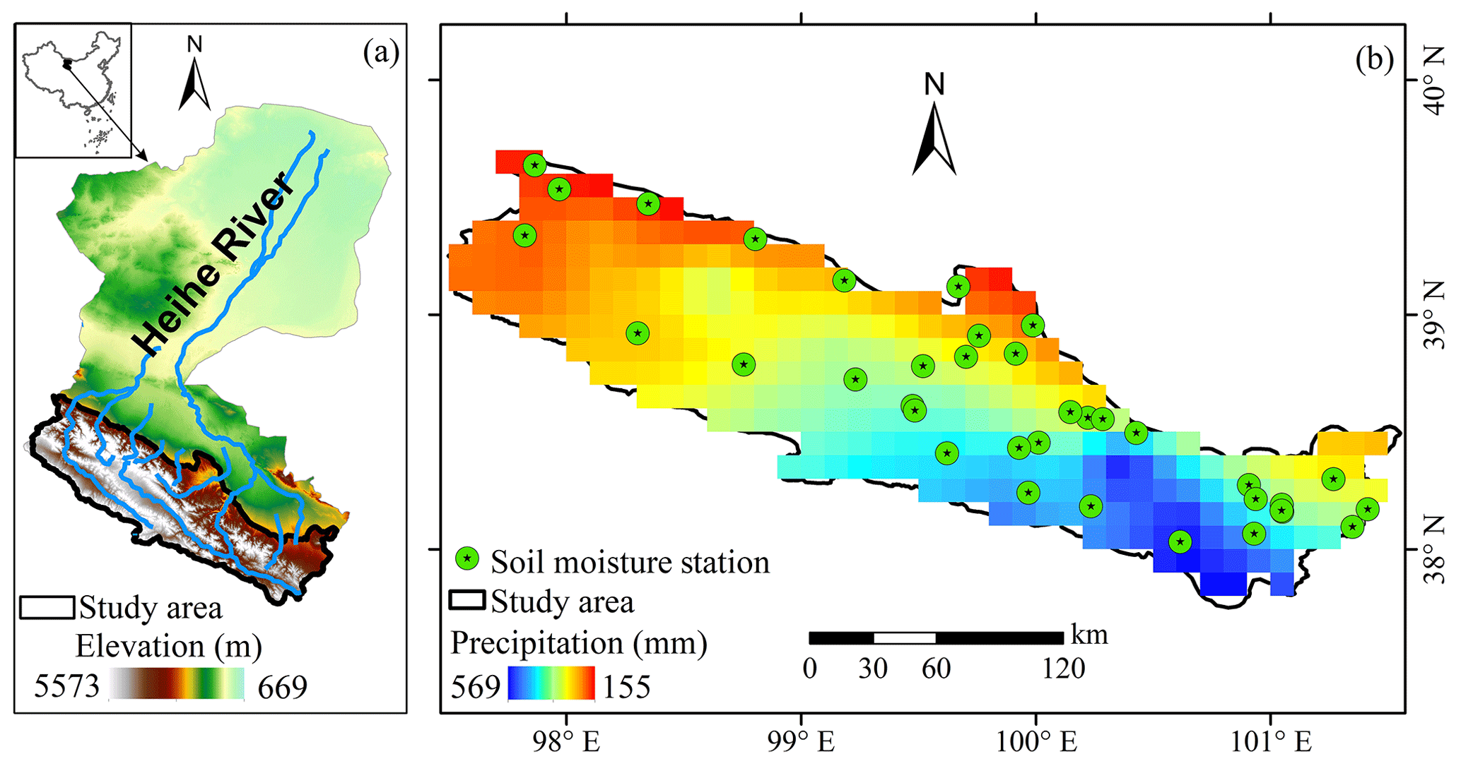
Figure 1(a) Study area and (b) distribution of the SM stations with spatial distribution of annual average precipitation from 2014 to 2016.
3.1 Datasets
We established a SM monitoring network in September 2013 in the Qilian Mountains. The network is composed of 35 SM stations distributed over the entire study area (Fig. 1). At each station, SM profiles from 0 to 70 cm were measured by soil moisture probes (ECH2O 5TE, METER Group Inc., USA) at 30 min intervals. These probes were installed at depths of 5 (representing a depth of 0 to 10 cm, SM5 cm), 15 (10 to 20 cm, SM15 cm), 25 (20 to 30 cm, SM25 cm), 40 (30 to 50 cm, SM40 cm), and 60 cm (50 to 70 cm, SM60 cm) below the soil surface. Soil-specific sensor calibrations were performed with the direct calibration method using soil samples taken from each station (Cobos and Chambers, 2010; Zhang et al., 2017b). The profile-integrated SM (SM0–70 cm) was calculated by the method of González-Zamora et al. (2016):
The entire dataset used in this study thus consists of six in situ SM time series at depths of 5, 15, 25, 40, 60, and 0 to 70 cm for each of the 35 stations. Due to the influence of soil freezing in winter, the soil moisture time series was limited to the growing seasons (May to October, Tian et al., 2019) of 2014, 2015, and 2016. The measurements were averaged to obtain daily SM, following the approach of Wagner et al. (1999). Data quality management was performed for each station, and data gaps existed in the harsh mountainous environment, as described in detail in Tian et al. (2019). Time series where more than 50 % of observations were missing were excluded from further analysis. The final dataset after processing is presented in Fig. 2. The surface SM measured at 5 cm was used to predict the subsurface SM at depths of 15, 25, 40, and 60 cm and the profile average (0 to 70 cm).
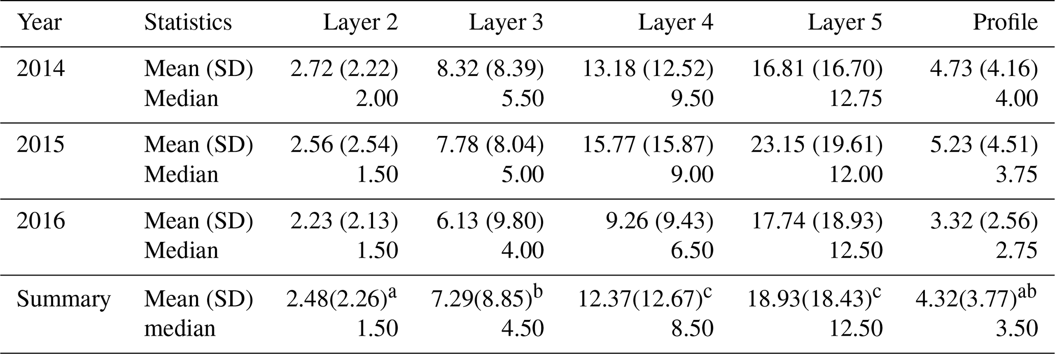
Soil cores were taken to measure soil properties, including soil organic carbon (SOC), saturated hydraulic conductivity (KS), soil particle composition, and bulk density for each layer during the sensor installation. Detailed descriptions of the soil properties can be found in Tian et al. (2017, 2019). The statistics of the soil physical characteristics are provided in Table 1. Daily reanalysis precipitation product (Chen et al., 2011) and Landsat-based continuous monthly 30 m ×30 m resolution NDVI data for the period 1986 to 2017 (Cihlar et al., 1994; Huete et al., 2002; Wu et al., 2019) were acquired from the National Tibetan Plateau Data Centre (https://data.tpdc.ac.cn/en/, last access: 18 September 2020).
The widely used higher-level SMAP_L3 Global Daily 9 km product for the growing seasons of 2015 to 2017 was used in this study. This product is distributed by NASA (http://nsidc.org/, last access: 18 September 2020) and described by O'Neill et al. (2018). SMAP descending node observations acquired near 06:00 local solar time have been combined with global daily composites in order to reduce the impact of Faraday rotation and to consider the assumption of uniform temperature profiles in the vegetation cover during morning overpasses. It has to be noted that the data are provided on a 9 km grid but that this is a result of a Backus–Gilbert optimal interpolation at brightness temperature level. The actual spatial resolution is coarser (O'Neill et al., 2018). The SMAP_L3 surface soil moisture product was also used to estimate the subsurface soil moisture (layer 2: 10 to 20 cm, layer 3: 20 to 30 cm, layer 4: 30 to 50 cm, layer 5: 50 to 70 cm) and profile soil moisture (0 to 70 cm) during the growing seasons of 2015 and 2016 in the mountainous area.
SMAP_L4 provides estimates of both surface and root zone SM products based on the assimilation of brightness temperature into the NASA land-surface model and has a spatial and temporal resolution of 9 km and 3 h, respectively (Reichle et al., 2017). SMAP_L4 is a widely used root zone SM product (Pablos et al., 2018). Here, the SMAP_L4 data were averaged to a daily resolution in order to compare it with the profile SM estimates from the SMAP_L3 surface product obtained in this study. In particular, the SMAP_L4 SM products with both surface (0 to 5 cm, sm0–5) and root zone (0 to 100 cm, sm0–100) information were used to calculate SM of the 0 to 70 cm profile (sm0–70) using
Table 1Statistics of the physical characteristics of the soil at the 35 soil moisture stations: mean (standard deviation).

Note: KS is the saturated hydraulic conductivity; SOC is the soil organic carbon.

Figure 2Daily soil moisture (vol. %) time series during the growing season of 2014 to 2016 for the five layers (layer 1, 0 to 10 cm; layer 2, 10 to 20 cm; layer 3, 20 to 30 cm; layer 4, 30 to 50 cm; layer 5, 50 to 70 cm) in the 35 soil moisture stations. Gaps exist for some stations due to missing data.
3.2 Exponential filter (ExpF) method
The ExpF method predicts the dynamics of subsurface SM using an exponential filter function of the surface SM dynamics (Wagner et al., 1999; Albergel et al., 2008). First, SM (cm3 cm−3) is transformed into a soil water index (SWI) with
where θi,min and θi,max are the minimum and maximum SM in the time series collected since installation for each layer at each station (Ford et al., 2014). The ExpF method then estimates subsurface SM from surface SM using
where SWI and SWI are the predicted subsurface SWI at time tn−1 and tn, respectively. ms is the observed surface SWI at time tn, and represents the gain at time tn calculated by
where is the gain at time tn−1 and T is the characteristic time in days. The equation was initialized with SWI and (Albergel et al., 2008). This method is particularly useful as T is the only unknown parameter. The optimum T (Topt) was determined by optimization using the highest Nash–Sutcliffe score for each specific depth at each station.
3.3 Artificial neural network (ANN) method
The ANN method is a data-driven method to predict subsurface SM from surface SM (Zhang et al., 2017a). If properly trained, an ANN can describe nonlinear relationships between dynamics of SM at different depths (Kornelsen and Coulibaly, 2014). The commonly used feed-forward ANN (with one hidden layer and 10 neurons, Levenberg–Marquardt algorithm, Ford et al., 2014) was used in this study. The ANN modeling was carried out using MATLAB (neural network time series tool, R2017b, The MathWorks). The output of the ANN was calculated using
where y is the output (the estimated subsurface soil moisture), f and g are the activation functions of the hidden layer and the input layer (the surface soil moisture), respectively, W1 and W2 are the weights of the input layer and the hidden layer, respectively, and b1 and b2 are the biases of the input layer and the hidden layer, respectively. The tangent sigmoid function was used as the activation function as it has shown good performance in hydrological studies (Yonaba et al., 2010). As suggested by Zhang et al. (2017a), 70 % of the data were selected for training the ANN and the remaining 30 % were used for validation. A separate ANN model was developed for every depth combination and every site.
3.4 Cumulative distribution function (CDF) matching method
In this study, the following procedure for CDF matching was used.
(1) Rank the surface (θ1) and the subsurface SM (θ2) time series.
(2) Calculate the difference between the two observation time series:
(3) Use a cubic polynomial fit to relate the difference (Δ) to surface SM (θ1) as recommended by Gao et al. (2019):
where is the predicted difference between surface and subsurface SM, and Ki () are parameters.
(4) Calculate CDF-matched subsurface SM (θCDF) with
Similarly to the ANN method, 70 % of the data were used to calibrate the approach, and the remaining 30 % of the data were used for validation of the CDF matching method.
3.5 Statistical analysis
Boxplots were used to show the scatter of the data. The difference between data in different groups was examined using a one-way analysis of variance (ANOVA) with the post hoc Bonferroni test when the normality and homogeneity of variance of the datasets were satisfied. The Kruskal–Wallis ANOVA with a post hoc Dunn's test was used in cases where these conditions were not satisfied (Lange et al., 2008). The statistical analysis was performed in SPSS (SPSS 18.0, SPSS Inc.) and Matlab (R2017b, The MathWorks). The significance level was 0.05 for all statistical tests.
4.1 Comparison of different methods
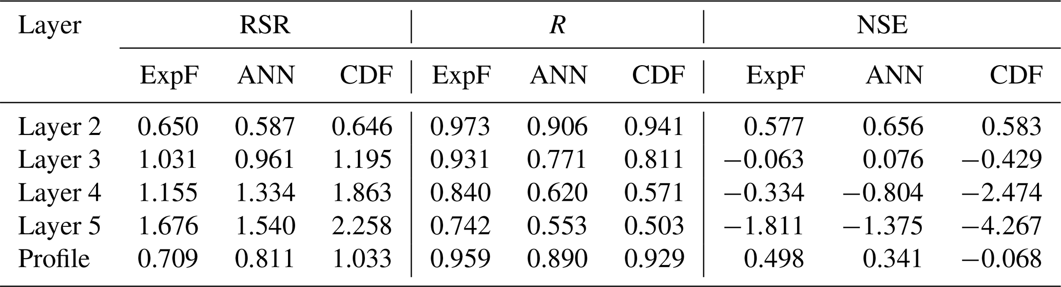
The ExpF method estimates subsurface SM based on SWI, while the ANN and CDF methods are based on volumetric soil moisture. Following Moriasi et al. (2007), the Nash–Sutcliffe efficiency (NSE), the ratio of RMSE to the standard deviation of the observations (RSR, an error statistic that normalizes the RMSE), and the Pearson correlation coefficient (R) were used to evaluate the performance of different methods with different units. To ensure that the comparison between the three methods is made under the same conditions, we divide the datasets into training data (the first 70 % of the data) and validation data (the remaining 30 % of the data) for all three methods. Figure 3 and Table 2 summarize the metrics (NSE, RSR, and R) for the subsurface SM estimates at different depths derived by the three different methods for the growing seasons of 2014, 2015, and 2016. Results show that ANN performed better than ExpF for the individual layers (layers 1 to 5) in terms of both NSE and RSR (Table 2 and Fig. 3), while ExpF performed better than ANN in estimating soil moisture for the entire soil profile. Additionally, the comparison of the performances between the ExpF and ANN methods was non-significant (p > 0.05) for all the layers, but ExpF showed a significantly (p < 0.05) higher R value compared to ANN for all the layers (with a median value of 0.97, 0.93, 0.84, 0.74, and 0.96 for layers 2, 3, 4, and 5, and profile SM, respectively). The good performance for R suggests that the ExpF method had the best ability to describe the temporal variability in SM. Furthermore, Table 2 and Fig. 3 indicate that CDF provided the worst performance among the three methods and thus cannot be recommended.
As expected, all metrics showed that the performance of the three methods decreased with depth. The results indicate that for two out of the three statistical measures (i.e., RSR and NSE), the ANN method was statistically superior to the other two methods. Specifically, the ANN method resulted in the lowest estimation error, while the ExpF method was better able to capture the SM dynamics. A similar finding was reported by Zhang et al. (2017a), who found that the ExpF method had a significantly higher correlation coefficient along with a higher mean bias compared to the ANN method. Furthermore, the ExpF method is a simpler approach as it only needs one parameter (Topt) and can thus be easily applied in data-scarce mountainous areas, while the establishment of the ANN method is much more complicated. In addition, the ExpF method is a process-based method, while ANN is a machine learning method. Therefore, the ExpF method was used to estimate the subsurface SM in the remainder of this study.
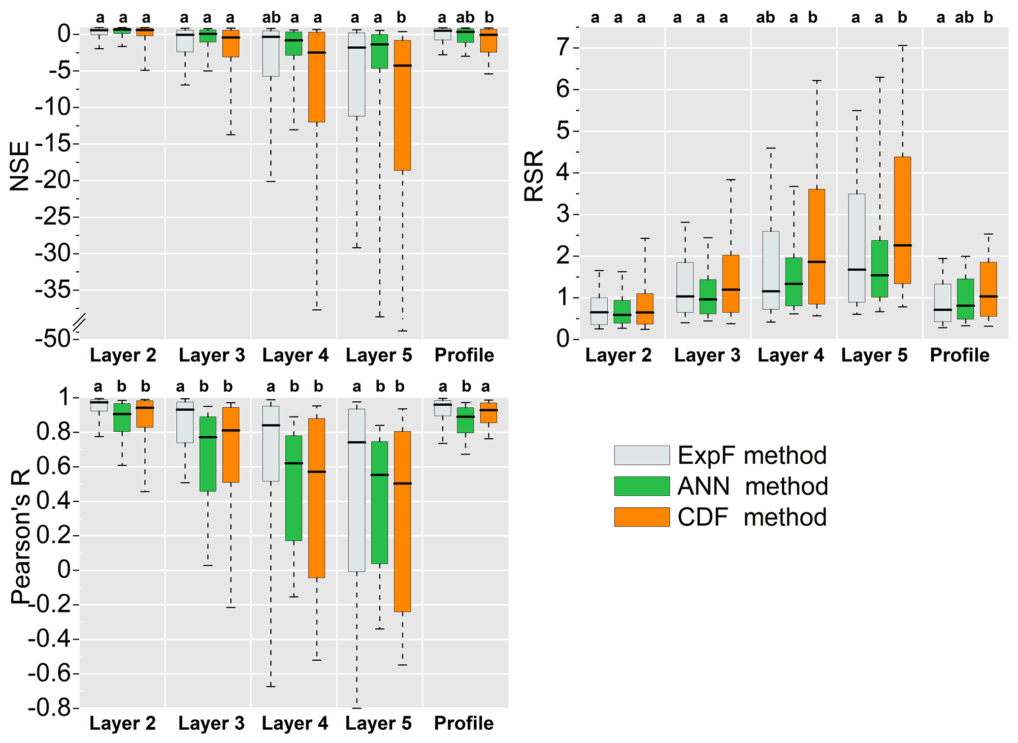
Figure 3Boxplot of the metrics (NSE, RSR, R) to compare the subsurface SM estimation using the surface SM by the three methods (ExpF, ANN, CDF) with the observations of the 35 stations during the growing seasons of 2014 to 2016. Different letters above the box indicate the significant difference (p < 0.05) among the different methods.
Table 2The median of the performance (RSR, R, and NSE) of the three different methods (ExpF, ANN, and CDF) for estimating the subsurface SM using the surface SM for each layer of 35 stations during the growing seasons of 2014, 2015, and 2016.
4.2 Evaluation of Topt for the ExpF method
4.2.1 Variation of Topt with depth
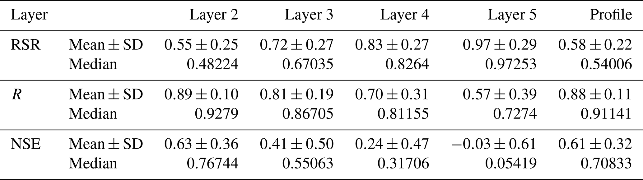
In the method comparison, the first 70 % and the remaining 30 % of data were selected as training and validation data, respectively, to ensure the comparison was under the same condition. However, for the standard procedure of the ExpF method in earlier studies, the entire dataset is always used to derive the Topt and validate the ExpF method (e.g., Wagner et al., 1999; Albergel et al., 2008; De Lange et al., 2008; Ford et al., 2014; Wang et al., 2017). Thus, the ExpF method is evaluated and analyzed using the entire dataset as well (performance of the ExpF method using the entire dataset was shown in Table 3 and Fig. S1 in the Supplement). Results indicate that the performances of ExpF in both layer 2 and profile are significantly higher than that of other layers. Moreover, results also indicate that the ExpF method showed good performance for layer 2 and profile SM (with median NSE > 0.65, median RSR < 0.60, Moriasi et al., 2007).
Table 3The statistics (mean±standard deviation and median) of the performance (RSR, R, and NSE) of the ExpF method for estimating the subsurface SM using the surface SM for each layer of 35 observation stations during the growing seasons of 2014, 2015, and 2016.
The accuracy of the ExpF method varied with the selected T value, and higher T values resulted in more stable estimations of SM time series (Wagner et al., 1999; Albergel et al., 2008). Furthermore, it was found that each station had an optimum T (Topt) as determined by the best match with observations in terms of NSE. The variation of NSE with T (ranging from 0 to 68 d) for different layers for each station is shown in Fig. 4 and Table 4. The sensitivity of high values of NSE to changes in T decreased with increasing depth, indicating that the range of T values with high NSE was larger deeper in the soil. This was also observed in previous studies (e.g., Wang et al., 2017).

Figure 4Variation of NSE with T of the exponential filter method for different layers at each station during the growing seasons of 2014, 2015, and 2016. The vertical axis is the NSE value. The frequency distribution curve and histogram show the distribution of Topt with depth for all stations.
Results of a two-way ANOVA showed that the difference of Topt is not significant between different years (p=0.06), while differences were significant between layers (p < 0.001). Furthermore, Topt increased with depth from layer 2 to layer 5. The median of Topt ranged from 1.5 d for layer 2 to 12.5 d for layer 5. The median Topt for profile SM was 3.5 d. Significant differences in Topt were obtained for layer 2, layer 3, and layer 4, but the difference between layers 4 and 5 was not significant. The increase in Topt with depth has already been observed in many studies and is related to the greater temporal stability of SM in deeper soil layers (Wang et al., 2017; Tian et al., 2019).
Table 4The statistics of Topt (day) for each layer and different year for all stations.
Note: SD represents the standard deviation. This summary represents the statistical result of the 3 years. Letters in the summary row indicate significant difference between respective layers: the same letter in each column indicates that the difference is nonsignificant, while different letters indicate a significant difference between the two layers (p < 0.05).
4.2.2 Evaluation of alternative methods for Topt estimation
Previous studies have used various methods to estimate Topt. For example, Albergel et al. (2008) and Ford et al. (2014) found that using a single representative value for Topt (e.g., average or median) for all stations did not significantly reduce the accuracy of the SM estimates. Wagner et al. (1999) recommended a common value of Topt=20 (d) to estimate root zone SM, and this value has been widely adopted (e.g., Lange et al., 2008; Muhammad et al., 2017). Qiu et al. (2014) proposed to estimate Topt using the station-specific long-term mean NDVI using (R=0.5, p < 0.01). This approach has also been applied in another study (Tobin et al., 2017).
Here, we evaluated four different methods to estimate Topt in our study region for estimating profile SM (0 to 70 cm, SWI) from surface SM (5 cm, SWI). In the first method, Topt was estimated from the NDVI-based regression of Qiu et al. (2014) to provide TQiu. In the second method, Topt was set to 20 d as recommended by Wagner et al. (1999) to provide TWagner. In the third method, an area-generalized Topt was obtained from the median value for the profile SM in our study region (3.5 d) to provide Tgeneral. In the fourth method, the original station-specific Topt parameter for profile SM was used (Tspecific). The accuracy of the SM estimates obtained using the different methods to estimate Topt was again evaluated using NSE, R, and RMSE (Fig. 5). The performance metrics show that Tspecific performed best (mean RSR of 0.58, R of 0.88, and NSE of 0.61), followed by Tgeneral (mean RSR of 0.61, R of 0.85, and NSE of 0.58), TWagner (mean RSR of 0.79, R of 0.69, and NSE of 0.32), and TQiu (mean RSR of 0.89, R of 0.59, and NSE of 0.17). However, the difference in performance between Tspecific and Tgeneral is not significantly different. The TWagner and TQiu approaches performed worse, and the metrics (NSE, R, RSR) are significantly (p < 0.001) lower than those of the Tgeneral and Tspecific methods. Our results suggest that a site-specific Topt significantly improves the performance of the ExpF method compared to the use of the universal Topt recommended by Wagner et al. (1999) or the regression of Qiu et al. (2014). Similarly, Lange et al. (2008) also found a significant improvement when using a station-specific Topt instead of Topt=20 d. It should be mentioned that the estimation depth in the method of Wagner et al. (1999) was 0 to 100 cm, while that of our study was 0 to 70 cm. This may partly explain the poor performance of the TWagner approach in this study. The use of an area-generalized Topt (3.5 d) is a suitable alternative to Topt estimation in our study area and provides similar estimation performance. Other studies have also found a good performance when using an area-generalized Topt (e.g., Albergel et al., 2008; Brocca et al., 2010; Ford et al., 2014).

Figure 5The boxplot of NSE, Pearson's R, and RSR for the Topt generated from different schemes. The different letters above each box indicate the significant difference for different schemes.
4.3 Estimating profile soil moisture using SMAP
The ExpF method is suitable for estimating the profile SM from the surface SM and the median of Topt is suitable for estimating subsurface soil moisture. Thus, in this section, we evaluate the utility of the ExpF method (with the median of Topt from SMAP) in combination with SMAP surface products for estimating subsurface SM in mountainous areas.
4.3.1 Assessment of the SMAP surface SM product
The observed surface SM of each station was compared with the SMAP_L3 soil moisture product that overlapped with the corresponding station for the growing seasons of 2015 and 2016 for all stations to evaluate the accuracy of the SMAP measurements (Pablos et al., 2018). The root mean square error (RMSE), mean bias error (MBE), unbiased RMSE (ubRMSE), and R were adopted as metrics to evaluate accuracy. The relationship between the SMAP_L3 SM data product and the in situ observations at 5 cm depth are presented in Fig. 6. Clearly, the larger deviation from linearity in the relationship is due to the scale discrepancy between the relatively large satellite footprints and the point location of in situ SM measurements. Nevertheless, the statistical metrics still indicate a significant relationship between the SMAP_L3 SM data product and the in situ observations at 5 cm depth. The time series of the two datasets for each station are provided in Fig. S2. Figures 6 and S2 show that the performance was low at two stations (D13 with R of 0.18, D15 with R of 0.08) with scrubland and relatively high soil moisture. The poor performance at scrubland sites is consistent with results presented by Zhang et al. (2017b) for this study region. Results showed that the MBE varied from −0.23 to 0.07 cm3 cm−3 with a median of −0.021 cm3 cm−3. This indicates that SMAP underestimated surface SM over the study region, which is consistent with previous studies in the area (Chen et al., 2017; Zhang et al., 2017b). The RMSE varied between 0.026 and 0.250 cm3 cm−3 between sites with a median value of 0.052 cm3 cm−3. After removing the bias, the SMAP product had a median ubRMSE of 0.036 cm3 cm−3 (range from 0.024 to 0.083 cm3/cm3). Therefore, the SMAP product achieved the accuracy requirement of 0.04 cm3 cm−3 (Chan et al., 2016) in this study area. The R value ranged from 0.075 to 0.81 with a median value of 0.59. The relationship between SMAP-derived and in situ observed surface SM was significant (p < 0.05) at all but one station. This suggests that the SMAP surface product can represent the temporal dynamics of the observed surface SM time series.
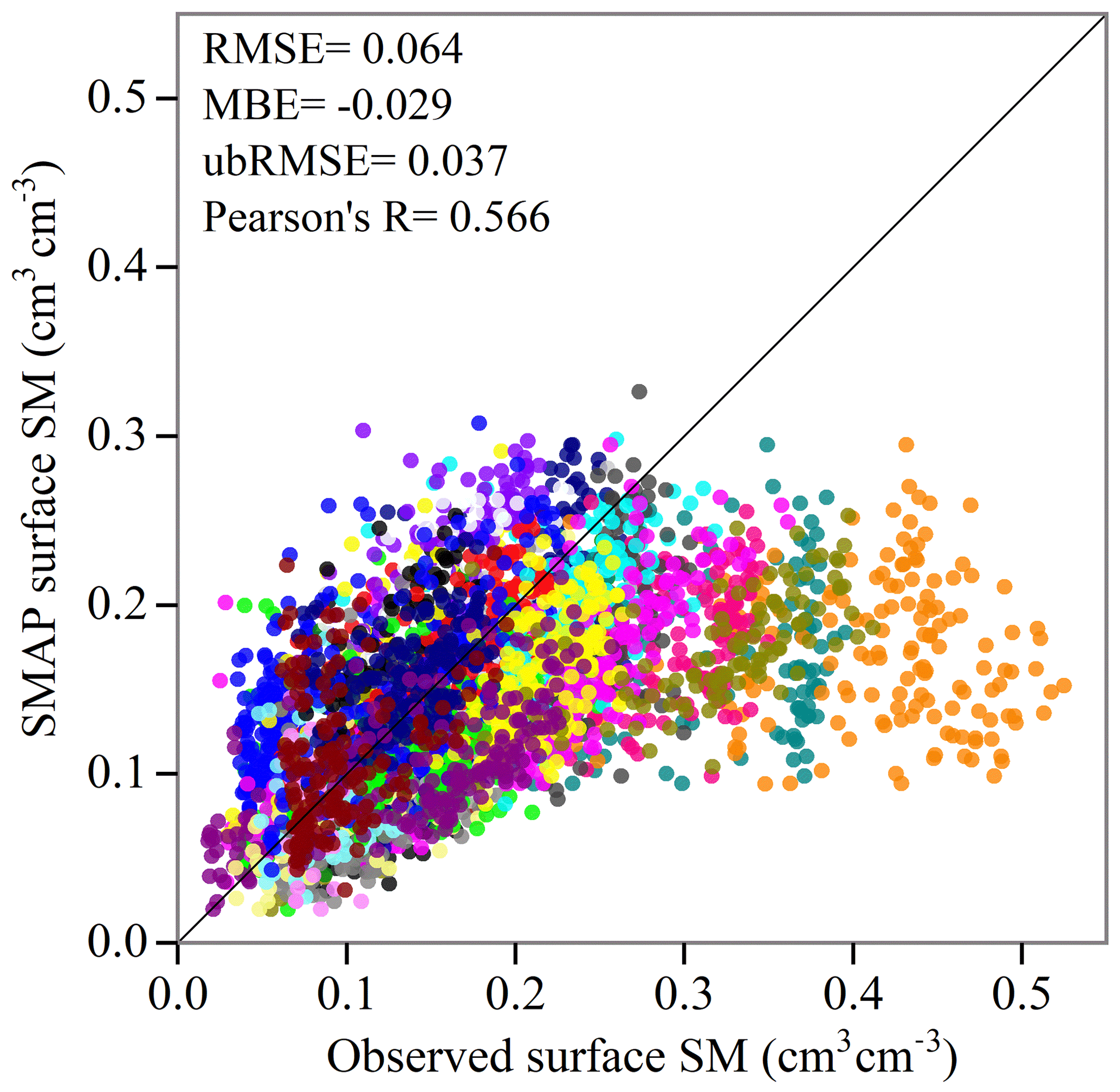
Figure 6The SMAP_L3 surface SM (cm3 cm−3) versus in situ observations at the surface (5 cm) for the 35 soil moisture stations. Color indicates station. The averaged metrics (RMSE, MBE, R, ubRMSE) are for all 35 stations during the growing seasons of 2015 and 2016.
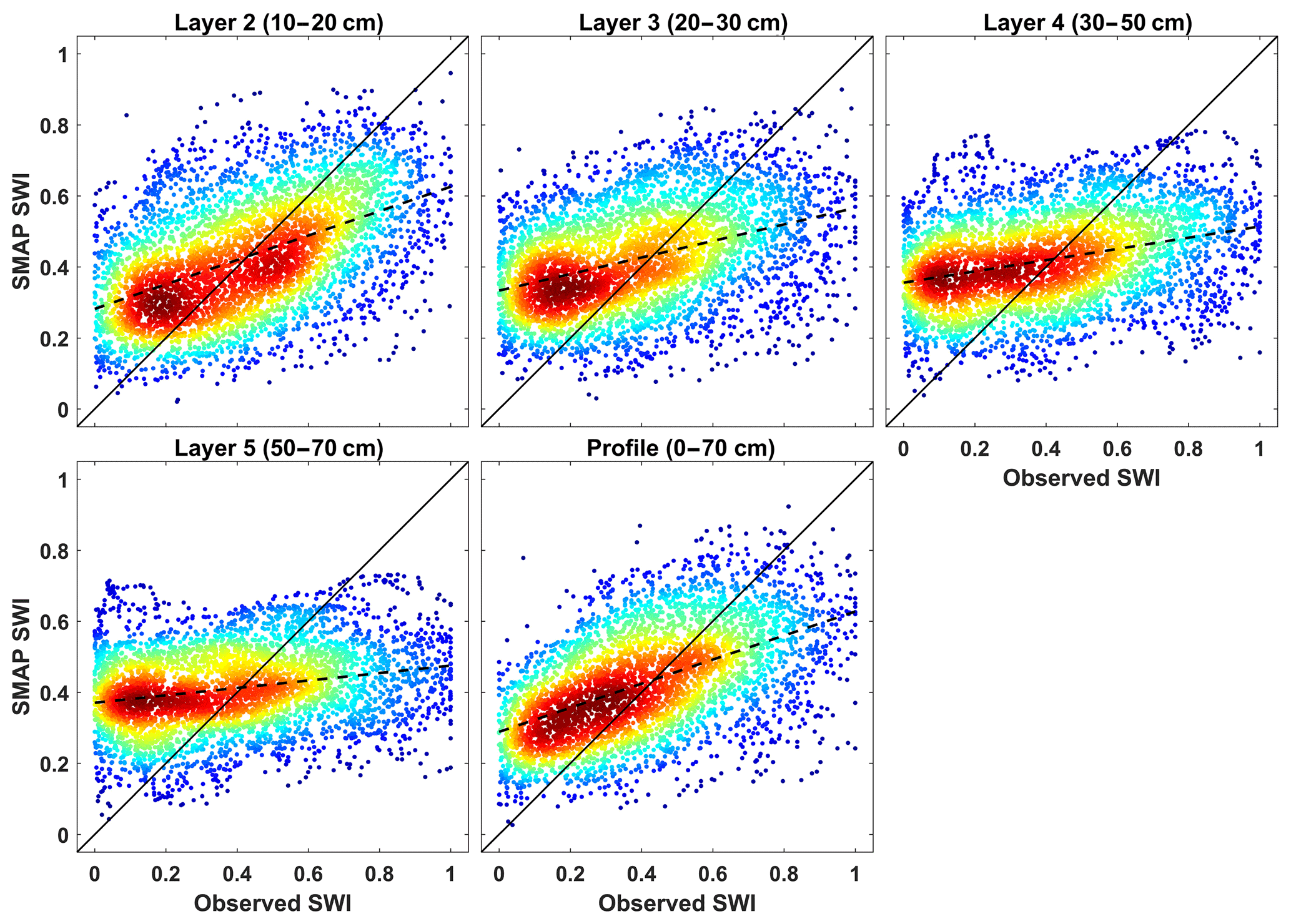
Figure 7Comparisons of SMAP_L3 estimated–observed subsurface SWI for all stations during the growing seasons of 2015 to 2016. The smoothed color density in the scatter plot shows the density of points more clearly. The dash and solid lines are the best-fitted curve and “y=x” line, respectively.
Table 5Performance metrics (RSR, R, NSE) for the comparison of SMAP estimated and observed SWI at different layers for the 35 stations during the growing seasons of 2015 to 2016.
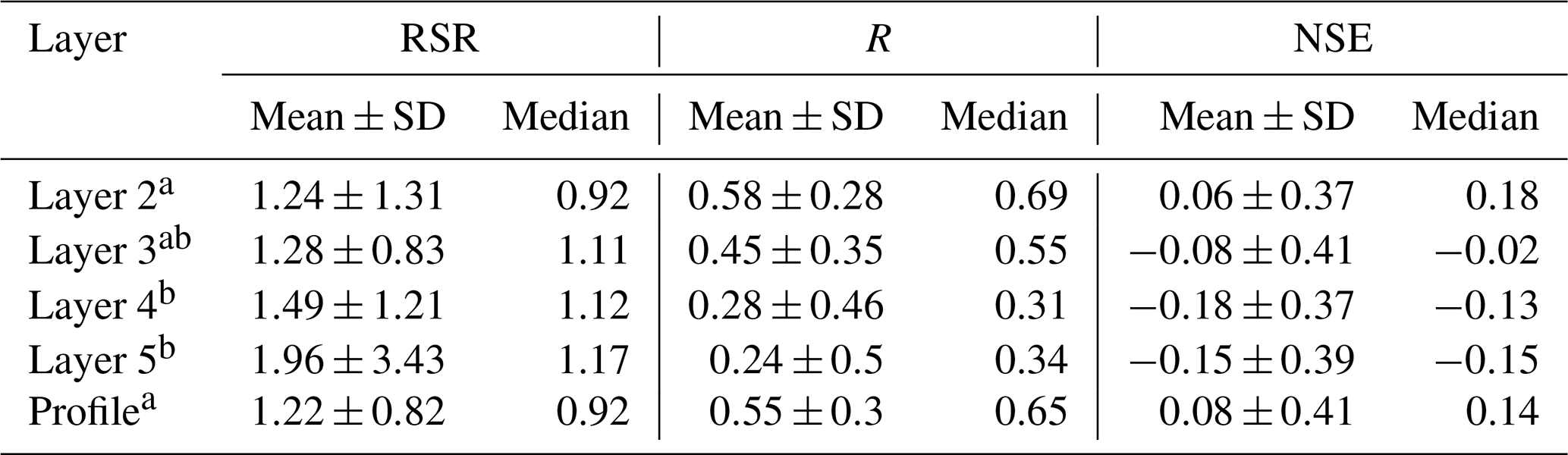
Note: the different letters after the layers indicate that the difference is significant at p < 0.05 (Kruskal–Wallis ANOVA).
Table 6Statistics of the metrics (RSR, R, NSE) of the comparisons of estimated–observed profile SWI datasets, SMAP_L3-observed surface SWI datasets, SMAP_L3-observed profile SWI datasets, and SMAP_L4-observed profile SWI datasets for the 35 stations during the growing seasons of 2015 and 2016.

Note: e.g., estimated–observed PSWI means the comparison of the estimated profile SWI and observed profile SWI.
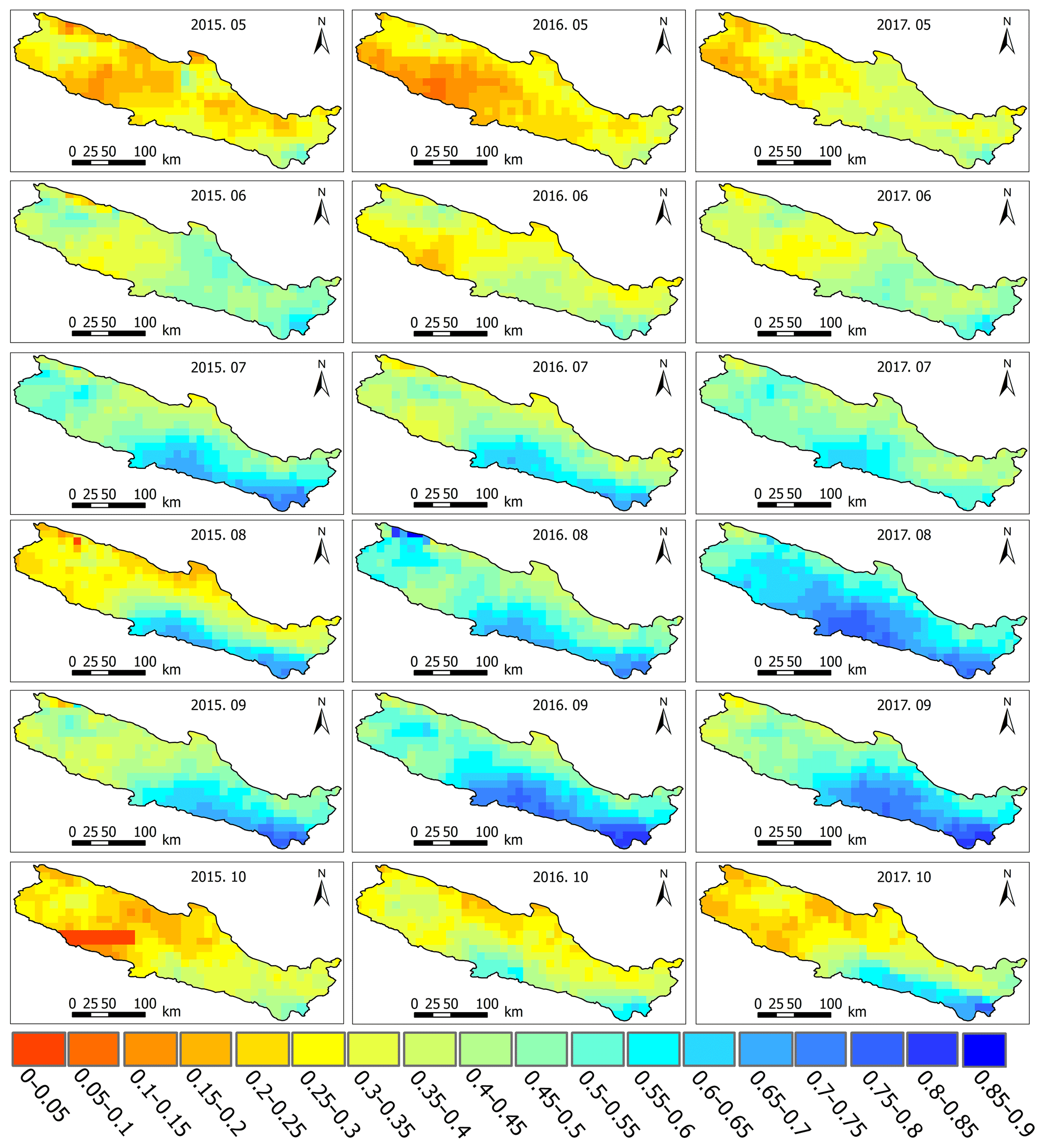
Figure 8The spatial distribution of the monthly averaged profile SWI product estimated from the SMAP_L3 surface product during the growing seasons from 2015 to 2017. The title of each subplot provides the month and year.
4.3.2 SMAP-based estimation of subsurface soil moisture
For the estimation of subsurface soil moisture from the SMAP_L3 surface product, the site-specific Topt was calculated based on the best match between SMAP estimations and in situ observations in terms of NSE. The median values of Topt for the layers 2, 3, 4, and 5 and the profile are 7, 12, 22, 35, and 10 d, respectively. The subsurface SWI estimated from the combination of SMAP surface SM with the ExpF method (with the median values of Topt) were compared with the in situ observations. A comparison of the subsurface SWI time series for different layers at each station are provided in Figs. S3 to S7. Figure 7 shows the measured SWI plotted against the predicted SWI. The performance metrics of these comparisons for each layer are summarized in Table 5.
As expected, the estimation accuracy of subsurface SM decreased with depth. The ANOVA results showed that the subsurface SM estimation accuracy for layer 2 (median value of RSR =0.92, R=0.69, NSE =0.18) and profile SM (RSR =0.92, R=0.65, NSE =0.14) was significantly higher than for layer 4 (RSR =1.12, R=0.31, NSE ) and layer 5 (RSR =1.17, R=0.34, NSE ) (p < 0.05). The NSE values were positive for layer 2 and profile SM, while the NSE values for the other layers were negative. The negative MBE shows that subsurface SM was underestimated. The relationship between SMAP-derived and in situ observed subsurface SM for layer 2 and profile SM was significant (p < 0.01) at all but one station (D15). Thus, the SMAP surface product and ExpF method can be used to estimate the subsurface SM in the study area, especially for layer 2 (10 to 20 cm) and profile (0 to 70 cm) SM.
As suggested by Ford et al. (2014), we partitioned the error in the SMAP-based estimation of profile SWI (“SMAP-observed profile SWI”, Fig. S8c) into errors associated with the ExpF method and errors due to SMAP observation differences to gain some insight into the error sources of SMAP-based estimates of profile SWI. For this, profile SWI estimated using the ExpF method from observed surface SWI was compared with in situ observed profile SWI (“estimated–observed profile SWI”) to assess errors of the ExpF method (Fig. S8a). In addition, SMAP-based and in situ observed surface SWIs (“SMAP-observed surface SWI”) were compared to assess inherent errors of the SMAP product (Fig. S8b). RMSE, R, and MAE were used as the metrics to assess accuracy. The results of this analysis are summarized in Table 6.
Figure S8 and Table 5 show that the SMAP-observed SWI had lower performance metrics for surface SWI (median values of RSR, R, and NSE are 1.01, 0.59, and −0.07, respectively) than for profile SWI (median values of RSR, R, and NSE are 0.88, 0.72, and 0.19, respectively), which was similar to the results obtained from the Nebraska SM network (Ford et al., 2014). This may be because the profile SWI was estimated based on the SMAP surface SWI and Topt, which was determined by optimization using the maximum NSE. This may have improved the performance of profile SWI estimation. In addition, the performance metrics for SMAP–observed SWI comparisons for both surface and profile SWI were significantly (p < 0.001) lower than those of estimated–observed profile SWI (median values of RSR, R, and NSE are 0.68, 0.90, and 0.64, respectively). Thus, the major error in SMAP-based profile SWI estimates stems from the SMAP satellite product and is not derived from the ExpF method, which is also supported by previous studies (e.g., Ford et al., 2014; Pablos et al., 2018). As mentioned before, the scale mismatch between point measurements and satellite footprints will introduce additional errors in the validation of the satellite-derived subsurface products (Jin et al., 2017).
Subsequently, the SMAP_L4 and SMAP_L3 estimated profile SWIs were compared to the in situ observed profile SWI (see Fig. S9 and Table 5). Table 5 shows that the performance of profile soil moisture estimation using the SMAP_L3 surface product and the ExpF method (median RSR, R, and NSE of 0.92, 0.65, and 0.14, respectively) was significantly (p < 0.01) better than that of the SMAP_L4 product (median RSR, R, and NSE of 1.25, 0.55, and −0.3, respectively). The low performance of the SMAP_L4 profile product may be associated with uncertainty in the meteorological driving forces and the soil parameters in the NASA catchment model for cold mountainous areas (Reichle et al., 2017; Zhao et al., 2018; Dai et al., 2019). Thus, our results suggest that combining the exponential filter method with the SMAP_L3 product significantly improves the estimation of profile SM for the data-scarce cold arid mountainous areas.
Finally, the spatial distribution of profile soil moisture during the growing seasons of 2015, 2016, and 2017 was obtained using the median value of Topt and the SMAP_L3 product to get the spatial distribution of profile SM in the study area (Fig. 8). Profile SM is higher in the southeast and lower in the northwestern part of the study area. This distribution coincides with the spatial distribution of precipitation and surface SM. The temporal variations of profile SWI, surface SWI, and precipitation are shown in Fig. S10. Figure S10 shows that the temporal variation of the SM profile corresponded well to the occurrence of precipitation: profile SM increased from May (mean SM of 0.27) to September (0.533) and then decreased until October (0.304). Profile SWISMAP (define SWISMAP before using it) was lower than surface SWISMAP from May to August, while profile SWISMAP was higher than surface SWISMAP from September to October. This can be attributed to the higher sensitivity of surface SM dynamics to precipitation and evapotranspiration (ET). During the months of September and October, less precipitation and higher ET caused a faster decrease in surface SM compared to profile SM.
Previous studies have shown the difficulty of applying the ExpF method to satellite products in mountainous areas, where complex topography (Paulik et al., 2014), snow, and soil freezing (Ford et al., 2014; Pablos et al., 2018) cause large errors and poor performance of the filtering method (Albergel et al., 2008). Ford et al. (2014) found an improvement of performance after removing the effects of snow from the data in the SCAN network, USA. In contrast, the present study showed that the ExpF method is useful in estimating profile SM from SMAP surface products in the growing season in high and cold mountainous areas, based on in situ SM observations.
We used three methods (the exponential filter (ExpF), the artificial neural network (ANN), and the cumulative distribution function matching (CDF) methods) to calculate subsurface SM from in situ surface SM observations at 5 cm depth in the Qilian Mountains (China). We also evaluated the utility of the ExpF method to estimate profile SM from SMAP surface products in the study area. Our main findings are the following.
-
With increasing depth of the predicted soil layer, the accuracies of all three methods decreased. The ExpF methods showed good performance for the estimation of SM down to 20 cm and profile.
-
The ANN method exhibited the lowest estimation error, while the ExpF approach captures the temporal variation of subsurface SM better than other methods.
-
The area-generalized Topt value of the ExpF method can be used in the study area to estimate the subsurface SM without significantly reducing the performance compared to a station-specific Topt.
-
Subsurface SM derived from the SMAP_L3 surface SM product using the ExpF method showed less deviation from the in situ observations compared to the SMAP_L4 root zone product for the study area.
We anticipate that our findings can improve the estimation of subsurface SM for large regions in mountainous areas, which in turn will support ecohydrological research and water resource management in inland river basins.
All the data used in this research are available upon request.
The supplement related to this article is available online at: https://doi.org/10.5194/hess-24-4659-2020-supplement.
BZ and CH prepared the research project. JT, ZH, CH, HRB, and JAH conceptualized the methodology. JT, ZH, and CM collected the data. JT, ZH, and HRB developed the code and performed the analysis. JT prepared the manuscript with contributions from all the co-authors.
The authors declare that they have no conflict of interest.
The project is partially funded by the National Natural Science Foundation of China (grants 41530752, 51609111, and 91125010) and Fundamental Research Funds for the Central Universities (lzujbky-2016-256). We are grateful to the members of the Center for Dryland Water Resources Research and Watershed Science, Lanzhou University, for their efforts to collect the soil moisture data and maintain the stations in this high, cold, and inaccessible mountainous area. Without their hard work, the soil moisture data presented in this paper would not have been available. We also thank the National Tibetan Plateau Data Centre (https://data.tpdc.ac.cn/en/, last access: 23 September 2020) for providing supporting data. The first author also wishes to express his appreciation for the assistance and friendship that he experienced during his stay at the Forschungszentrum Jülich from September 2017 to March 2019.
This research has been supported by the National Natural Science Foundation of China (grant nos. 41530752 and 91125010), the 111 Project (grant no. P2018001) and the Fundamental Research Funds for the Central Universities (lzujbky-2016-256).
This paper was edited by Nunzio Romano and reviewed by Salvatore Manfreda and two anonymous referees.
Albergel, C., Rüdiger, C., Pellarin, T., Calvet, J.-C., Fritz, N., Froissard, F., Suquia, D., Petitpa, A., Piguet, B., and Martin, E.: From near-surface to root-zone soil moisture using an exponential filter: an assessment of the method based on in-situ observations and model simulations, Hydrol. Earth Syst. Sci., 12, 1323–1337, https://doi.org/10.5194/hess-12-1323-2008, 2008.
Bojinski, S., Verstraete, M., Peterson, T. C., Richter, C., Simmons, A., and Zemp, M.: The concept of essential climate variables in support of climate research, applications, and policy, B. Am. Meteorol. Soc., 95, 1431–1443, https://doi.org/10.1175/bams-d-13-00047.1, 2014.
Brocca, L., Melone, F., Moramarco, T., Wagner, W., Naeimi, V., Bartalis, Z., and Hasenauer, S.: Improving runoff prediction through the assimilation of the ASCAT soil moisture product, Hydrol. Earth Syst. Sci., 14, 1881–1893, https://doi.org/10.5194/hess-14-1881-2010, 2010.
Brocca, L., Ciabatta, L., Massari, C., Camici, S., and Tarpanelli, A.: Soil Moisture for Hydrological Applications: Open Questions and New Opportunities, Water, 9, 140, https://doi.org/10.3390/w9020140, 2017.
Ceballos, A., Scipal, K., Wagner, W., and Martinez-Fernandez, J.: Validation of ERS scatterometer-derived soil moisture data in the central part of the Duero Basin, Spain, Hydrol. Process., 19, 1549–1566, https://doi.org/10.1002/hyp.5585, 2005.
Chan, S. K., Bindlish, R., O'Neill, P. E., Njoku, E., Jackson, T., Colliander, A., Chen, F., Burgin, M., Dunbar, S., and Piepmeier, J.: Assessment of the SMAP passive soil moisture product, IEEE T. Geosci. Remote, 54, 4994–5007, https://doi.org/10.1109/TGRS.2016.2561938, 2016.
Chen, Y., Yang, K., He, J., Qin, J., Shi, J., Du, J., and He, Q.: Improving land surface temperature modeling for dry land of China, J. Geophys. Res.-Atmos., 116, D20104, https://doi.org/10.1029/2011jd015921, 2011.
Chen, Y., Yang, K., Qin, J., Cui, Q., Lu, H., La, Z., Han, M., and Tang, W.: Evaluation of SMAP, SMOS and AMSR2 soil moisture retrievals against observations from two networks on the Tibetan Plateau, J. Geophys. Res.-Atmos., 122, 5780–5792, https://doi.org/10.1002/2016JD026388, 2017.
Cihlar, J., Manak, D., and D'Iorio, M.: Evaluation of Compositing Algorithms for AVHRR Data over Land, IEEE T. Geosci. Remote, 32, 427–437. https://doi.org/10.1109/36.295057, 1994.
Cobos, D. R. and Chambers, C.: Calibrating ECH2O soil moisture sensors, Application Note, Decagon Devices, Pullman, WA, 2010.
Colliander, A., Jackson, T. J., Bindlish, R., Chan, S., Das, N., Kim, S., Cosh, M., Dunbar, R., Dang, L., and Pashaian, L.: Validation of SMAP surface soil moisture products with core validation sites, Remote Sens. Environ., 191, 215–231, https://doi.org/10.1016/j.rse.2017.01.021, 2017.
Dai, Y., Shangguan, W., Wei, N., Xin, Q., Yuan, H., Zhang, S., Liu, S., Lu, X., Wang, D., and Yan, F.: A review of the global soil property maps for Earth system models, SOIL, 5, 137–158, https://doi.org/10.5194/soil-5-137-2019, 2019.
De Lannoy, G. J. M., Houser, P. R., Verhoest, N. E. C., Pauwels, V. R. N., and Gish, T. J.: Upscaling of point soil moisture measurements to field averages at the OPE3 test site, J. Hydrol., 343, 1–11, https://doi.org/10.1016/j.jhydrol.2007.06.004, 2007.
Dobriyal, P., Qureshi, A., Badola, R., and Hussain, S. A.: A review of the methods available for estimating soil moisture and its implications for water resource management, J. Hydrol., 458, 110–117, https://doi.org/10.1016/j.jhydrol.2012.06.021, 2012.
Drusch, M., Wood, E. F., and Gao, H.: Observation operators for the direct assimilation of TRMM microwave imager retrieved soil moisture, Geophys. Res. Lett., 32, L15403, https://doi.org/10.1029/2005GL023623, 2005.
Entekhabi, D., Yueh, S., ONeill, P. E., Kellogg, K. H., Allen, A., Bindlish, R., Brown, M., Chan, S., Colliander, A., and Crow, W. T.: SMAP handbook-Soil Moisture Active Passive: Mapping Soil Moisture and Freeze/Thaw From Space, Jet Propulsion Lab., California Inst. Technol., Pasadena, California, 2014.
Escorihuela, M.-J., Chanzy, A., Wigneron, J.-P., and Kerr, Y.: Effective soil moisture sampling depth of L-band radiometry: A case study, Remote Sens. Environ., 114, 995–1001, https://doi.org/10.1016/j.rse.2009.12.011, 2010.
Feng, Q., Yang, L., Deo, R. C., AghaKouchak, A., Adamowski, J. F., Stone, R., Yin, Z., Liu, W., Si, J., Wen, X., Zhu, M., and Cao, S.: Domino effect of climate change over two millennia in ancient China's Hexi Corridor, Nat. Sustainability, 2, 957–961, https://doi.org/10.1038/s41893-019-0397-9, 2019.
Ford, T. W., Harris, E., and Quiring, S. M.: Estimating root zone soil moisture using near-surface observations from SMOS, Hydrol. Earth Syst. Sci., 18, 139–154, https://doi.org/10.5194/hess-18-139-2014, 2014.
Gao, X., Li, H., Zhao, X., Ma, W., and Wu, P.: Identifying a suitable revegetation technique for soil restoration on water-limited and degraded land: Considering both deep soil moisture deficit and soil organic carbon sequestration, Geoderma, 319, 61–69, https://doi.org/10.1016/j.geoderma.2018.01.003, 2018.
Gao, X., Zhao, X., Brocca, L., Pan, D., and Wu, P.: Testing of observation operators designed to estimate profile soil moisture from surface measurements, Hydrol. Process., 33, 575–584, https://doi.org/10.1002/hyp.13344, 2019.
Georgakakos, K. P., Bae, D.-H., and Cayan, D. R.: Hydroclimatology of Continental Watersheds: 1. Temporal Analyses, Water Resour. Res., 31, 655–675, https://doi.org/10.1029/94WR02375, 1995.
González-Zamora, Á., Sánchez, N., Martínez-Fernández, J., and Wagner, W.: Root-zone plant available water estimation using the SMOS-derived soil water index, Adv. Water Resour., 96, 339–353, https://doi.org/10.1016/j.advwatres.2016.08.001, 2016.
Green, J. K., Seneviratne, S. I., Berg, A. M., Findell, K. L., Hagemann, S., Lawrence, D. M., and Gentine, P.: Large influence of soil moisture on long-term terrestrial carbon uptake, Nature, 565, 476–479, https://doi.org/10.1038/s41586-018-0848-x, 2019.
Han, E., Heathman, G. C., Merwade, V., and Cosh, M. H.: Application of observation operators for field scale soil moisture averages and variances in agricultural landscapes, J. Hydrol., 444–445, 34–50, https://doi.org/10.1016/j.jhydrol.2012.03.035, 2012.
Han, X., Hendricks Franssen, H.-J., Li, X., Zhang, Y., Montzka, C., and Vereecken, H.: Joint assimilation of surface temperature and L-band microwave brightness temperature in land data assimilation, Vadose Zone J., 12, L19501, https://doi.org/10.2136/vzj2012.0072, 2013.
He, C. S., Zhang, L. H., and Wang, Y.: Impacts of Heterogeneity of Soil Hydraulic Properties on Watershed Hydrological Processes, Science Press, Beijing, 2018 (in Chinese with Engligh abstract).
Huete, A., Didan, K., Miura, T., Rodriguez, E. P., Gao, X., and Ferreira, L. G.: Overview of The Radiometric and Biophysical Performance of The MODIS Vegetation Indices, Remote Sens. Environ., 83, 195–213, 10.1016/s0034-4257(02)00096-2, 2002.
Jakobi, J., Huisman, J., Vereecken, H., Diekkrüger, B., and Bogena, H.: Cosmic Ray Neutron Sensing for Simultaneous Soil Water Content and Biomass Quantification in Drought Conditions, Water Resour. Res., 54, 7383–7402, https://doi.org/10.1029/2018wr022692, 2018.
Jin, R., Li, X., and Liu, S. M.: Understanding the Heterogeneity of Soil Moisture and Evapotranspiration Using Multiscale Observations From Satellites, Airborne Sensors, and a Ground-Based Observation Matrix, IEEE Geosci. Remote Sens. Lett., 14, 2132–2136, https://doi.org/10.1109/LGRS.2017.2754961, 2017.
Jin, X., Zhang, L. h., Gu, J., Zhao, C., Tian, J., and He, C. S.: Modeling the impacts of spatial heterogeneity in soil hydraulic properties on hydrological process in the upper reach of the Heihe River in the Qilian Mountains, Northwest China, Hydrol. Process., 29, 3318–3327, 10.1002/hyp.10437, 2015.
Jonard, F., Bogena, H., Caterina, D., Garré, S., Klotzsche, A., Monerris, A., Schwank, M., and von Hebel, C.: Ground-Based Soil Moisture Determination, in: Observation and Measurement, edited by: Li, X. and Vereecken, H., Springer, Berlin, Heidelberg, 1–42, 2018.
Jung, M., Reichstein, M., Ciais, P., Seneviratne, S. I., Sheffield, J., Goulden, M. L., Bonan, G., Cescatti, A., Chen, J., de Jeu, R., Dolman, A. J., Eugster, W., Gerten, D., Gianelle, D., Gobron, N., Heinke, J., Kimball, J., Law, B. E., Montagnani, L., Mu, Q., Mueller, B., Oleson, K., Papale, D., Richardson, A. D., Roupsard, O., Running, S., Tomelleri, E., Viovy, N., Weber, U., Williams, C., Wood, E., Zaehle, S., and Zhang, K.: Recent decline in the global land evapotranspiration trend due to limited moisture supply, Nature, 467, 951, https://doi.org/10.1038/nature09396, 2010.
Kornelsen, K. C. and Coulibaly, P.: Root-zone soil moisture estimation using data-driven methods, Water Resour. Res., 50, 2946–2962, https://doi.org/10.1002/2013WR014127, 2014.
Lange, R. D., Beck, R., Giesen, N. v. d., Friesen, J., Wit, A. d., and Wagner, W.: Scatterometer-Derived Soil Moisture Calibrated for Soil Texture With a One-Dimensional Water-Flow Model, IEEE T. Geosci. Remote, 46, 4041–4049, https://doi.org/10.1109/TGRS.2008.2000796, 2008.
Li, X., Liu, S., Xiao, Q., Ma, M., Jin, R., Che, T., Wang, W., Hu, X., Xu, Z., and Wen, J.: A multiscale dataset for understanding complex eco-hydrological processes in a heterogeneous oasis system, Sci. Data, 4, 170083, https://doi.org/10.1038/sdata.2017.83, 2017.
Li, X., Cheng, G. D., Ge, Y. C., Li, H. Y., Han, F., Hu, X. L., Tian, W., Tian, Y., Pan, X. D., Nian, Y. Y., Zhang, Y. L., Ran, Y. H., Zheng, Y., Gao, B., Yang, D. W., Zheng, C. M., Wang, X. S., Liu, S. M., and Cai, X. M.: Hydrological Cycle in the Heihe River Basin and Its Implication for Water Resource Management in Endorheic Basins, J. Geophys. Res.-Atmos., 123, 890–914, https://doi.org/10.1002/2017jd027889, 2018.
Li, Z., Xu, Z., Shao, Q., and Yang, J.: Parameter estimation and uncertainty analysis of SWAT model in upper reaches of the Heihe river basin, Hydrol. Process., 23, 2744–2753, https://doi.org/10.1002/hyp.7371, 2009.
Liu, H., Zhao, W., He, Z., and Liu, J.: Soil moisture dynamics across landscape types in an arid inland river basin of Northwest China, Hydrol. Process., 29, 3328–3341, https://doi.org/10.1002/hyp.10444, 2015.
Liu, J., Chai, L., Lu, Z., Liu, S., Qu, Y., Geng, D., Song, Y., Guan, Y., Guo, Z., and Wang, J.: Evaluation of SMAP, SMOS-IC, FY3B, JAXA, and LPRM Soil Moisture Products over the Qinghai-Tibet Plateau and Its Surrounding Areas, Remote Sens., 11, 792, https://doi.org/10.3390/rs11070792, 2019.
Liu, S., Li, X., Xu, Z., Che, T., Xiao, Q., Ma, M., Liu, Q., Jin, R., Guo, J., Wang, L., Wang, W., Qi, Y., Li, H., Xu, T., Ran, Y., Hu, X., Shi, S., Zhu, Z., Tan, J., Zhang, Y., and Ren, Z.: The Heihe Integrated Observatory Network: A Basin-Scale Land Surface Processes Observatory in China, Vadose Zone J., 17, 1–21, https://doi.org/10.2136/vzj2018.04.0072, 2018a.
Liu, Z., Cheng, L., Hao, Z., Li, J., Thorstensen, A., and Gao, H.: A framework for exploring joint effects of conditional factors on compound floods, Water Resour. Res., 54, 2681–2696, 2018b.
Luo, K., Tao, F., Moiwo, J. P., and Xiao, D.: Attribution of hydrological change in Heihe River Basin to climate and land use change in the past three decades, Sci. Rep.-UK, 6, 33704, https://doi.org/10.1038/srep33704, 2016.
Mahmood, R. and Hubbard, K. G.: Relationship between soil moisture of near surface and multiple depths of the root zone under heterogeneous land uses and varying hydroclimatic conditions, Hydrol. Process., 21, 3449–3462, https://doi.org/10.1002/hyp.6578, 2007.
Manfreda, S., Brocca, L., Moramarco, T., Melone, F., and Sheffield, J.: A physically based approach for the estimation of root-zone soil moisture from surface measurements, Hydrol. Earth Syst. Sci., 18, 1199–1212, https://doi.org/10.5194/hess-18-1199-2014, 2014.
Moriasi, D. N., Arnold, J. G., Van Liew, M. W., Bingner, R. L., Harmel, R. D., and Veith, T. L.: Model evaluation guidelines for systematic quantification of accuracy in watershed simulations, T. ASABE, 50, 885–900, https://doi.org/10.13031/2013.23153, 2007.
Muhammad, Z., Hyunglok, K., and Minha, C.: Evaluating the patterns of spatiotemporal trends of root zone soil moisture in major climate regions in East Asia, J. Geophys. Res.-Atmos., 122, 7705–7722, https://doi.org/10.1002/2016JD026379, 2017.
Ochsner, T. E., Cosh, M. H., Cuenca, R. H., Dorigo, W. A., Draper, C. S., Hagimoto, Y., Kerr, Y. H., Larson, K. M., Njoku, E. G., Small, E. E., and Zreda, M.: State of the Art in Large-Scale Soil Moisture Monitoring, Soil Sci. Soc. Am. J., 77, 1888–1919, https://doi.org/10.2136/sssaj2013.03.0093, 2013.
Pablos, M., González-Zamora, Á., Sánchez, N., and Martínez-Fernández, J.: Assessment of Root Zone Soil Moisture Estimations from SMAP, SMOS and MODIS Observations, Remote Sens., 10, 981, https://doi.org/10.3390/rs10070981, 2018.
Pan, Q. M. and Tian, S. L.: Water resources in the Heihe river basin, The Yellow River Water Conservency Press, Zheng Zhou, China, 2001 (in Chinese).
Pan, X., Kornelsen, K. C., and Coulibaly, P.: Estimating Root Zone Soil Moisture at Continental Scale Using Neural Networks, J. Am. Water Resour. Assoc., 53, 220–237, https://doi.org/10.1111/1752-1688.12491, 2017.
Pasolli, L., Notarnicola, C., Bruzzone, L., Bertoldi, G., Della Chiesa, S., Hell, V., Niedrist, G., Tappeiner, U., Zebisch, M., and Del Frate, F.: Estimation of soil moisture in an alpine catchment with RADARSAT2 images, Appl. Environ. Soil Sci., 2011, 341–366, https://doi.org/10.1155/2011/175473, 2011.
Paulik, C., Dorigo, W., Wagner, W., and Kidd, R.: Validation of the ASCAT Soil Water Index using in situ data from the International Soil Moisture Network, Int. J. Appl. Earth Obs, 30, 1–8, https://doi.org/10.1016/j.jag.2014.01.007, 2014.
Peng, J., Loew, A., Merlin, O., and Verhoest, N. E.: A review of spatial downscaling of satellite remotely sensed soil moisture, Rev. Geophys., 55, 341–366, https://doi.org/10.1002/2016RG000543, 2017.
Qiu, J. X., Crow, W. T., Nearing, G. S., Mo, X. G., and Liu, S. X.: The impact of vertical measurement depth on the information content of soil moisture times series data, Geophys. Res. Lett., 41, 4997–5004, https://doi.org/10.1002/2014gl060017, 2014.
Qu, Y., Zhu, Z., Chai, L., Liu, S., Montzka, C., Liu, J., Yang, X., Lu, Z., Jin, R., and Li, X.: Rebuilding a Microwave Soil Moisture Product Using Random Forest Adopting AMSR-E/AMSR2 Brightness Temperature and SMAP over the Qinghai–Tibet Plateau, China, Remote Sens., 11, 683, https://doi.org/10.3390/rs11060683, 2019.
Rasmy, M., Koike, T., Boussetta, S., Lu, H., and Li, X.: Development of a satellite land data assimilation system coupled with a mesoscale model in the Tibetan Plateau, IEEE T. Geosci. Remote, 49, 2847–2862, https://doi.org/10.1109/TGRS.2011.2112667, 2011.
Reichle, R. H. and Koster, R. D.: Bias reduction in short records of satellite soil moisture, Geophys. Res. Lett., 31, https://doi.org/10.1029/2004GL020938, 2004.
Reichle, R. H., Lannoy, G. J. M. D., Liu, Q., Ardizzone, J. V., Colliander, A., Conaty, A., Crow, W., Jackson, T. J., Jones, L. A., Kimball, J. S., Koster, R. D., Mahanama, S. P., Smith, E. B., Berg, A., Bircher, S., Bosch, D., Caldwell, T. G., Cosh, M., González-Zamora, Á., Collins, C. D. H., Jensen, K. H., Livingston, S., Lopez-Baeza, E., Martínez-Fernández, J., McNairn, H., Moghaddam, M., Pacheco, A., Pellarin, T., Prueger, J., Rowlandson, T., Seyfried, M., Starks, P., Su, Z., Thibeault, M., Velde, R. v. d., Walker, J., Wu, X., and Zeng, Y.: Assessment of the SMAP Level-4 Surface and Root-Zone Soil Moisture Product Using In Situ Measurements, J. Hydrometeorol., 18, 2621–2645, https://doi.org/10.1175/jhm-d-17-0063.1, 2017.
Seneviratne, S. I., Corti, T., Davin, E. L., Hirschi, M., Jaeger, E. B., Lehner, I., Orlowsky, B., and Teuling, A. J.: Investigating soil moisture–climate interactions in a changing climate: a review, Earth Sci. Rev., 99, 125–161, https://doi.org/10.1016/j.earscirev.2010.02.004, 2010.
Tian, J., Zhang, B., He, C., and Yang, L.: Variability in Soil Hydraulic Conductivity and Soil Hydrological Response Under Different Land Covers in the Mountainous Area of the Heihe River Watershed, Northwest China, Land Degrad. Dev., 28, 1437–1449, https://doi.org/10.1002/ldr.2665, 2017.
Tian, J., Zhang, B., He, C., Han, Z., Bogena, H. R., and Huisman, J. A.: Dynamic response patterns of profile soil moisture wetting events under different land covers in the Mountainous area of the Heihe River Watershed, Northwest China, Agr. Forest Meteorol., 271, 225–239, https://doi.org/10.1016/j.agrformet.2019.03.006, 2019.
Tobin, K. J., Torres, R., Crow, W. T., and Bennett, M. E.: Multi-decadal analysis of root-zone soil moisture applying the exponential filter across CONUS, Hydrol. Earth Syst. Sci., 21, 4403–4417, https://doi.org/10.5194/hess-21-4403-2017, 2017.
Ullah, W., Wang, G., Gao, Z., Hagan, D. F. T., and Lou, D.: Comparisons of remote sensing and reanalysis soil moisture products over the Tibetan Plateau, China, Cold Reg. Sci. Technol., 146, 110–121, https://doi.org/10.1016/j.coldregions.2017.12.003, 2018.
Wagner, W., Lemoine, G., and Rott, H.: A method for estimating soil moisture from ERS scatterometer and soil data, Remote Sens. Environ., 70, 191–207, https://doi.org/10.1016/s0034-4257(99)00036-x, 1999.
Wang, S., Fu, B., Gao, G., Zhou, J., Jiao, L., and Liu, J.: Linking the soil moisture distribution pattern to dynamic processes along slope transects in the Loess Plateau, China, Environ. Monit. Assess., 187, 778, https://doi.org/10.1007/s10661-015-5000-x, 2015.
Wang, T., Franz, T. E., You, J., Shulski, M. D., and Ray, C.: Evaluating controls of soil properties and climatic conditions on the use of an exponential filter for converting near surface to root zone soil moisture contents, J. Hydrol., 548, 683–696, https://doi.org/10.1016/j.jhydrol.2017.03.055, 2017.
Williams, C., McNamara, J., and Chandler, D.: Controls on the temporal and spatial variability of soil moisture in a mountainous landscape: the signature of snow and complex terrain, Hydrol. Earth Syst. Sci., 13, 1325–1336, https://doi.org/10.5194/hess-13-1325-2009, 2009.
Wu, J., Zhong, B., and Wu, J.: Landsat-based continuous monthly 30 m ×30 m land surface NDVI dataset in Qilian Mountain area (1986–2017), National Tibetan Plateau Data Center, https://doi.org/10.11888/Geogra.tpdc.270136, 2019.
Wu, W., Geller, M. A., and Dickinson, R. E.: The response of soil moisture to long-term variability of precipitation, J. Hydrometeorol., 3, 604–613, https://doi.org/10.1175/1525-7541(2002)003<0604:TROSMT>2.0.CO;2, 2002.
Pan, X., Kornelsen, K. C., and Coulibaly, P.: Estimating Root Zone Soil Moisture at Continental Scale Using Neural Networks, J. Am. Water Resour. Assoc., 53, 220–237, https://doi.org/10.1111/1752-1688.12491, 2017.
Yao, Y., Zheng, C., Andrews, C., Zheng, Y., Zhang, A., and Liu, J.: What Controls the Partitioning between Baseflow and Mountain Block Recharge in the Qinghai-Tibet Plateau?, Geophys. Res. Lett., 44, 8352–8358, https://doi.org/10.1002/2017GL074344, 2017.
Zeng, J., Li, Z., Chen, Q., Bi, H., Qiu, J., and Zou, P.: Evaluation of remotely sensed and reanalysis soil moisture products over the Tibetan Plateau using in-situ observations, Remote Sens. Environ., 163, 91–110, https://doi.org/10.1016/j.rse.2015.03.008, 2015.
Zhang, L., He, C., and Zhang, M.: Multi-Scale Evaluation of the SMAP Product Using Sparse In-Situ Network over a High Mountainous Watershed, Northwest China, Remote Sens., 9, 1111, https://doi.org/10.3390/rs9111111, 2017b.
Zhang, N., Quiring, S., Ochsner, T., and Ford, T.: Comparison of Three Methods for Vertical Extrapolation of Soil Moisture in Oklahoma, Vadose Zone J., 16, 1–9, https://doi.org/10.2136/vzj2017.04.0085, 2017a.
Zhao, H., Zeng, Y., Lv, S., and Su, Z.: Analysis of soil hydraulic and thermal properties for land surface modeling over the Tibetan Plateau, Earth Syst. Sci. Data, 10, 1031–1061, https://doi.org/10.5194/essd-10-1031-2018, 2018.
Zhao, L., Yang, K., Qin, J., Chen, Y., Tang, W., Montzka, C., Wu, H., Lin, C., Han, M., and Vereecken, H.: Spatiotemporal analysis of soil moisture observations within a Tibetan mesoscale area and its implication to regional soil moisture measurements, J. Hydrol., 482, 92–104, https://doi.org/10.1016/j.jhydrol.2012.12.033, 2013.
Zhao, L., Yang, K., Qin, J., Chen, Y., Tang, W., Lu, H., and Yang, Z.-L.: The scale-dependence of SMOS soil moisture accuracy and its improvement through land data assimilation in the central Tibetan Plateau, Remote Sens. Environ., 152, 345–355, https://doi.org/10.1016/j.rse.2014.07.005, 2014.
Zhao, W. and Li, A.: A comparison study on empirical microwave soil moisture downscaling methods based on the integration of microwave-optical/IR data on the Tibetan Plateau, Int. J. Remote Sens., 36, 4986–5002, https://doi.org/10.1080/01431161.2015.1041178, 2015.
Zhou, J., Cai, W., Qin, Y., Lai, L., Guan, T., Zhang, X., Jiang, L., Du, H., Yang, D., Cong, Z., and Zheng, Y.: Alpine vegetation phenology dynamic over 16 years and its covariation with climate in a semi-arid region of China, Sci. Total Environ., 572, 119–128, https://doi.org/10.1016/j.scitotenv.2016.07.206, 2016.