the Creative Commons Attribution 4.0 License.
the Creative Commons Attribution 4.0 License.
 | 22 Sep 2020
An uncertainty partition approach for inferring interactive hydrologic risks
Kai Huang
Guohe Huang
Yongping Li
Feng Wang
Extensive uncertainties exist in hydrologic risk analysis. Particularly for interdependent hydrometeorological extremes, the random features in individual variables and their dependence structures may lead to bias and uncertainty in future risk inferences. In this study, an iterative factorial copula (IFC) approach is proposed to quantify parameter uncertainties and further reveal their contributions to predictive uncertainties in risk inferences. Specifically, an iterative factorial analysis (IFA) approach is developed to diminish the effect of the sample size and provide reliable characterization for parameters' contributions to the resulting risk inferences. The proposed approach is applied to multivariate flood risk inference for the Wei River basin to demonstrate the applicability of IFC for tracking the major contributors to resulting uncertainty in a multivariate risk analysis framework. In detail, the multivariate risk model associated with flood peak and volume will be established and further introduced into the proposed iterative factorial analysis framework to reveal the individual and interactive effects of parameter uncertainties on the predictive uncertainties in the resulting risk inferences. The results suggest that uncertainties in risk inferences would mainly be attributed to some parameters of the marginal distributions, while the parameter of the dependence structure (i.e. copula function) would not produce noticeable effects. Moreover, compared with traditional factorial analysis (FA), the proposed IFA approach would produce a more reliable visualization for parameters' impacts on risk inferences, while the traditional FA would remarkably overestimate the contribution of parameters' interaction to the failure probability in AND (i.e. all variables would exceed the corresponding thresholds) and at the same time underestimate the contribution of parameters' interaction to the failure probabilities in OR (i.e. one variable would exceed its corresponding threshold) and Kendall (i.e. the correlated variables would exceed a critical multivariate threshold).
- Article
(4344 KB) - Full-text XML
- BibTeX
- EndNote


Many hydrological and climatological extremes are highly correlated with each other, and it is desired to explore their interdependence through multivariate approaches. Examples include sea-level rise and fluvial flood (Moftakhari et al., 2017), drought and heat waves (Sun et al., 2019), and soil moisture and precipitation (AghaKouchak, 2015). Moreover, even one specific hydrological extreme may have multiple attributes, such as the peak and volume for a flood, duration and severity for a drought, and duration and intensity of a storm (Karmakar and Simonovic, 2009; Kong et al., 2019). Traditional univariate approaches, mainly focusing on one variable or one attribute of hydrological extremes (e.g. flood peak), may not be sufficient to describe those hydrological extremes containing multivariate characteristics. Thus the univariate frequency/risk analysis methods may be unable to obtain reliable risk inferences for the failure probability or recurrence intervals of interdependent extreme events (Chebana and Ouarda, 2011; Requena et al., 2013; Salvadori et al., 2016; Sadegh et al., 2017).
Since the introduction of the copula function into hydrology and the geosciences by De Michele and Salvadori (2003), the copula-based approaches have been widely used for multivariate hydrologic risk analysis. The copula functions are able to model correlated variables with complex or nonlinear dependence structures. Also, these kinds of methods are easily implemented since the marginal distributions and dependence models can be estimated in separate processes which also give flexibility in the selection of both marginal and dependence models. A large amount of research has been developed for multivariate hydrologic simulation through copula functions, such as multivariate flood frequency analysis (Sraj et al., 2014; Xu et al., 2016; Fan et al., 2018, 2020); drought assessments (Song and Singh, 2010; Kao and Govindaraju, 2010; Ma et al., 2013); storm or rainfall dependence analysis (Zhang and Singh, 2007; Vandenberghe et al., 2010); streamflow simulation (Lee and Salas, 2011; Kong et al., 2015); and other water and environmental engineering applications (Fan et al., 2017; Huang et al., 2017).
For both univariate and multivariate analyses for hydrometeorological risks, uncertainty would be one of the unavoidable issues which needs to be well addressed. The uncertainty in hydrometeorological risk inference mainly results from stochastic variability of hydrometeorological processes and incomplete knowledge of the watershed systems (Merz and Thieken, 2005). Many studies have been proposed to address uncertainty in both univariate and multivariate hydrological risk analysis (e.g. Merz and Thieken, 2005; Serinaldi, 2013; Dung et al., 2015; Zhang et al., 2015; Sadegh et al., 2017; Fan et al., 2018). However, one critical issue in uncertainty quantification of hydrological inference is how to characterize the major sources for uncertain risk inference. Qi et al. (2016) employed a subsampling ANOVA approach (Bosshard et al., 2013) to quantify individual and interactive impacts of the uncertainties in data, probability distribution functions, and probability distribution parameters on the total cost for flood control in terms of flood peak flows. Even though the subsampling ANOVA approach is able to reduce the effect of the biased estimator on quantification of variance contribution resulting from the traditional ANOVA approach, it should be noticed that merely subsampling one uncertainty parameter/factor (referred to as single-subsampling ANOVA), as used in the studies by Bosshard et al. (2013) and Qi et al. (2016a), will lead to (i) an underestimation of the individual contribution for the factor to be sampled and (ii) overestimation of contributions from those non-sampled factors. Moreover, few studies have been reported to characterize the individual and interactive effects of parameter uncertainties in marginal and dependence models on the multivariate risk inferences.
Consequently, as an extension of previous research, this study aims to propose an iterative factorial copula (IFC) approach for quantifying and partitioning uncertainty metrics from different sources in multivariate hydrologic risk inference. In detail, the parameter uncertainties are quantified through a Monte Carlo based bootstrap algorithm. The interactions of parameter uncertainties are explored through a multilevel factorial analysis approach. The contributions of parameter uncertainties are analysed through an iterative factorial analysis (IFA) method, in which all uncertainty factors will be subsampled to generate more reliable results. The applicability of the proposed IFC approach will be demonstrated through case studies of flood risk analysis in the Wei River basin in China.
Figure 1 illustrates the framework of the proposed IFC approach. The framework consists of four modules: (i) selection of marginal distributions, (ii) identification of copulas, (iii) parameter uncertainty quantification, and (iv) parameter interaction and sensitivity analysis. In IFC, modules (i) and (ii) are proposed to construct the most appropriate copula-based hydrologic risk model. In detail, a number of distributions, such as Gamma, generalized extreme value (GEV), lognormal (LN), Pearson type III (P III), and log-Pearson type III (LP III) distributions, are usually employed to describe the probabilistic features of individual random variables (e.g. flood peak and volume). Also, in order to quantify the dependence structures of correlated random variables, many copula functions have been proposed, such as Gaussian copula, Student t copula, and the Archimedean copula family (e.g. Clayton, Gumbel, Frank, and Joe copulas). In the current study, the indices of root mean square error (RMSE) and Akaike information criterion (AIC) will be employed to identify the most appropriate model for hydrologic risk inference. Module (iii) quantifies parameter uncertainties in marginal distributions and copulas. Module (iv) would be the core part of our study to identify the main sources of uncertainties in multivariate risk inference by the proposed iterative factorial analysis (IFA) approach.

2.1 Copula-based multivariate risk inference framework
A copula function is a multivariate distribution function with uniform margins on the interval [0, 1]. Sklar's theorem states that any d-dimensional distribution function F can be formulated through a copula and its marginal distributions (Nelsen, 2006). In detail, a multivariate copula function can be expressed as
where are marginal distributions of the random vector (X1, X2, …, Xd), with γ1, γ2, …, γd, respectively, being the unknown parameters of the marginal distributions. θ is the parameter in the copula function describing dependence among the correlated variables. If these marginal distributions are continuous, then a single copula function C exists, which can be written as (Nelsen, 2006)
where , , …, . More details on the theoretical background and properties of various copula families can be found in Nelsen (2006).
If appropriate copula functions are specified to reflect the joint probabilistic characteristics for a multivariate extreme event, the conditional, primary, and secondary return periods (RPs) can be obtained. Consider one kind of hydrological extreme (denoted as X) with d attributes (i.e. X=(x1, x2, …, xd)), and for a specific extreme event X* with its attributes being (, , …, ), three categories of multivariate RP can be applied to determine the potential risk of X*.
(i) “OR” case TOR:
where Rd is a d-dimensional real space; μ denotes the average time between two adjacent events under consideration. The joint RP in OR (denoted as TOR) indicates the occurrence probability of the extreme event with one of its variables, xi, i=1, 2, …, d, exceeding the corresponding threshold .
(ii) “AND” case TAND:
where is the multivariate survival function of the Xi proposed by Salvadori et al. (2013, 2016), and . Following Salvadori et al. (2013, 2016) and the inclusion–exclusion principle proposed by Joe (2014), the multivariate survival function can be obtained by
and
where #(S) denotes the cardinality of S. The joint RP in AND (denoted as TAND) of the extreme event indicates the occurrence probability with all of its variables xi, i=1, 2, …, d, exceeding the corresponding thresholds .
(iii) “Kendall” case: the Kendall RP characterizes the hydrologic disasters exceeding a critical layer as defined by Salvadori et al. (2011): . The Kendall RP can be expressed as (Salvadori et al., 2011)
where KC is the Kendall distribution function associated with the copula C, which can be expressed as
In addition to the multivariate RP, failure probability (FP) can be another index to provide more coherent, general, and well-devised tools for multivariate risk assessment and communication. In general, the failure probability pM to indicate the occurrence of a critical event for at least one time in M years of design life can be defined as (Salvadori et al., 2016)
Similar to the multivariate RP concept, the failure probability in a multivariate context can also be characterized in the “OR”, “AND”, and “Kendall” scenarios expressed by the following equations. For a given critical threshold , the failure probabilities violating this critical value can be expressed as (Salvadori et al., 2016)
where , , and , respectively, denote the failure probability in the “AND”, “OR”, and “Kendall” cases. T indicates the service time of the facilities under consideration.
Focusing on a bivariate case, the joint RP and the associated failure probability in the “OR”, “AND”, and “Kendall” scenarios can be formulated as (Salvadori et al., 2007, 2011; Graler et al., 2013; Sraj et al., 2014; Serinaldi, 2015)
where , , , and , (, define the bivariate threshold.
2.2 Uncertainty in the copula-based risk model
Extensive uncertainties may be involved in the parametric estimation of a copula function due to (i) the inherent uncertainty in the flooding process; (ii) uncertainty in the selection of appropriate marginal functions and copulas; and (iii) statistical uncertainty or parameter uncertainty within the parameter estimation process (e.g. the availability of samples) (Zhang et al., 2015). Several methods have been proposed to quantify parameter uncertainties in copula-based models. For instance, Dung et al. (2015) proposed bootstrap-based methods for quantifying the parameter uncertainties in bivariate copula models. Zhang et al. (2015) employed a Bayesian inference approach for evaluating uncertainties in copula-based hydrologic drought models, in which the component-wise hit-and-run Metropolis algorithm is adopted to estimate the posterior probabilities of model parameters.
In this study, a bootstrap-based algorithm is applied to quantify parameter uncertainties in the copula-based multivariate risk model. The procedures describing the bootstrap-based algorithm to derive probabilistic distributions of the parameters in both marginal and dependence models are presented as follows.
-
Predefine a large number of bootstrapping samplings NB.
-
Implement the resampling with replacement over observed pairs Z= (X, Y) to obtain (X*, Y*); Z* has the same size as Z.
-
Fit the chosen marginal distributions to X* and Y* and estimate the associated parameters (γX,γY).
-
Fit the chosen copula to Z* and estimate the parameter in the copula function θ.
-
Repeat steps 2–5 NB times and obtain NB sets of ). Moreover, in order to reject those parameters that lead to bad fits for both marginal and copula models, the A–D test and the Cramér–von Mises test are introduced in the bootstrap procedure to ensure that the obtained parameters can pass statistical tests for both the marginal distribution and copula models. Then the kernel method will be adopted to quantify the probabilistic features for γX, γY, and θ.
-
In order to derive bivariate uncertainty bands for a predefined quantile curve (QC) with certain joint RP in “AND”, “OR”, or “Kendall” (denoted as TAND, TOR, and TKendall), sample sets of from the obtained NB samples.
-
Sample a large number (Ns) of xi yj from their marginal distributions.
-
For each set of from , evaluate the joint RPs of (xi, yj) (i=1, 2, …, Ns; y=1, 2, …, Ns) and store the pairs of (xi, yj) approaching the predefined joint RPs.
-
Repeat step 8 for and for each predefined QC and plot the bivariate uncertainty bands for each quantile QC.
2.3 Interactive and sensitivity analysis for parameter uncertainties
Due to the uncertainties existing in the unknown values of parameters for a copula model, the associated risk or the return period for a flooding event may also be uncertain. Few studies have been reported to analyse the effect of uncertainties in the copula model on evaluating the risk for a flood event. To address the above issue, an iterative factorial analysis (IFA) approach will be proposed to reveal the individual and interactive effects of parameter uncertainties on the predictive uncertainties of different risk inferences.
Consider a copula-based bivariate risk assessment model which has two marginal distributions (A and B) and one copula (C). The parameters in the two marginal distributions are assumed to be, respectively, denoted as γA with a levels and γB with b levels, while the parameter in the copula is denoted with θC with c levels. The three-factor ANOVA model for such a factorial design in terms of the predictive risk (denoted as R) in response to the parameters γA, γB, and θC and n replicates can be expressed as
where R0 denotes the overall mean effect; , and , respectively, indicate the effect for parameter θC in the copula at the ith level, parameter γA in the first marginal distribution at the jth level, and parameter γB in the first marginal distribution at the kth level; , and indicate interactions between factors θC and γA, θC and γB, as well as γA and γB, respectively; denotes the interaction of factors θC , γA, and γB; εijkl denotes the random error component.
Based on Eq. (12), the total variability of the predictive risk can be decomposed into its component parts as follows (Montgomery, 2001):
and
where , , , , and . Then the contributions of parameter uncertainties in marginal distributions and dependence structures can be calculated as the following.
(3) Contribution of parameters in marginal distributions A and B:
(2) Contribution of the parameter in the dependence structure:
(3) Contribution of internal variability:
(4) Contribution of parameter interactions:
However, one major issue for the ANOVA approach is that the biased variance estimator in ANOVA would underestimate the variance in small sample size scenarios (Bosshard et al., 2013). Thus the sample size may significantly affect the resulting variance contributions expressed in Eqs. (14a)–(14e). A subsampling approach has been advanced by Bosshard et al. (2013) to diminish the effect of the sample size in ANOVA and has been employed for uncertainty partitioning in flood design and hydrological simulation (Qi et al., 2016a, b). In such a subsampling scheme, one factor (denoted as X) with T levels (these levels can be different values for numerical parameters, or different types for non-numerical factors, e.g. model type) would choose two levels in each iteration. For T possible levels of X, we can obtain a total of possible pairs for X, expressed as a matrix as follows:
However, such a subsampling approach is mainly applied to subsample merely one factor or one parameter (here we refer to this method as single-subsampling ANOVA) in previous studies (Bosshard et al., 2013; Qi et al., 2016a, b). However, a critical issue for the single-subsampling ANOVA is that it will lead to an underestimation of the individual contribution for the factor to be sampled and overestimation of contributions for those non-sampled factors. Consequently, in this study, we will propose an IFA approach to subsample all the factors to be addressed and then quantify the contribution of each factor to the response variation. In the IFA approach, all factors under consideration will be subsampled, and the corresponding sum of squares will be obtained. The contribution of one factor would be characterized by the mean value of its contribution in each iteration. In detail, for the three-factor ANOVA model expressed by Eq. (12), the subsampling schemes for the three parameters can be formulated as
Consequently, there are a total number of iterations in IFA for the three-factor model expressed as Eq. (12). For each iteration, the sums of squares can be reformulated as
where . . Also, for each iteration, the corresponding contributions for each factor can be obtained as
Finally, the individual and interactive contributions for those factors can be obtained by averaging the corresponding contributions in all iterations, expressed as
where .
The proposed IFC approach can be applied to various multivariate risk inference problems. In this study, we will apply IFC for multivariate flood risk inference at the Wei River basin in China. The Weihe River plays a key role in the economic development of western China and thus is known regionally as the “Mother River” of the Guanzhong Plain of the southern part of the Loess Plateau (Song et al., 2007; Zuo et al., 2014; Du et al., 2015, Xu et al., 2016). It originates from the Niaoshu mountain at an elevation of 3485 m above mean sea level in Weiyuan County of Gansu Province (Du et al., 2015). The Weihe River basin is characterized by a semi-arid and sub-humid continental monsoon climate, resulting in significant temporal–spatial variations in precipitation, with an annual average precipitation of 559 mm (Xu et al., 2016). Furthermore, there is a strong decreasing gradient from south to north in which the southern region experiences a sub-humid climate with annual precipitation ranging from 800 to 1000 mm, whereas the northern region has a semi-arid climate with annual precipitation ranging from 400 to 700 mm (Xu et al., 2016). Over the entire basin, the mean temperature ranges from 6 to 14 ∘C, the annual potential evapotranspiration fluctuates from 660 to 1600, and the annual actual evapotranspiration is about 500 mm (Du et al., 2015).
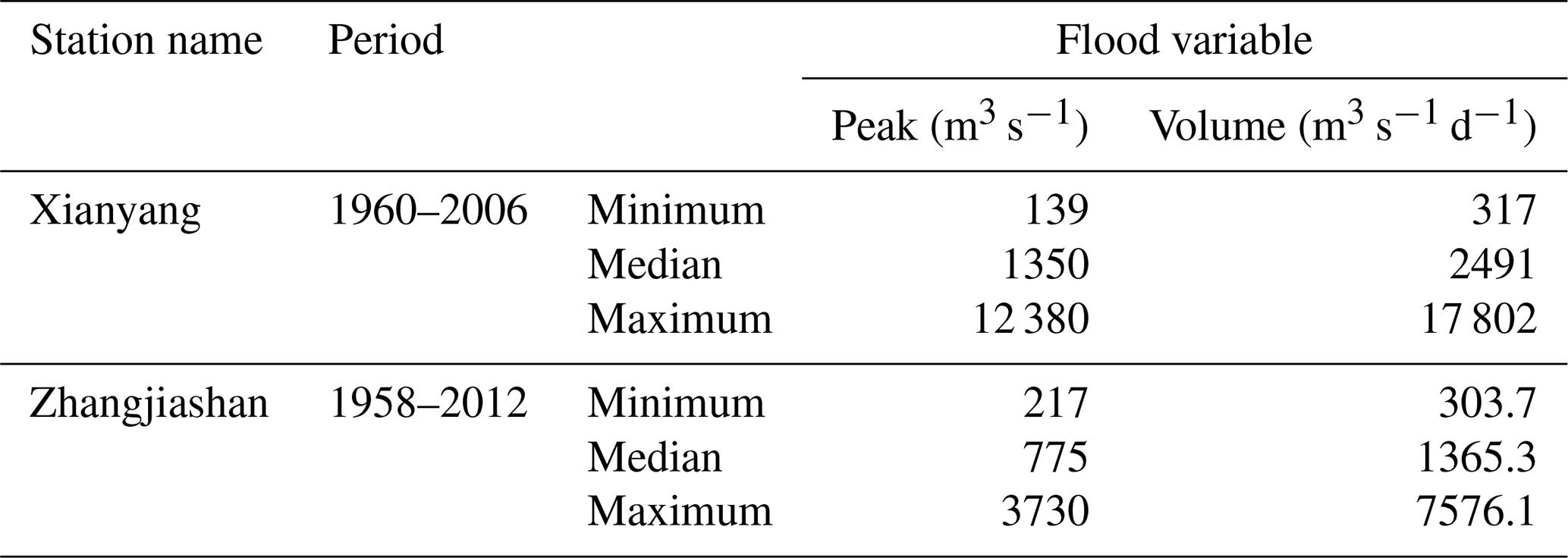
Observed daily streamflow data at the Xianyang and Zhangjiashan gauging stations were used for hydrologic risk analysis. Figure 2 shows the locations of these two gauging stations based on the daily streamflow data, the flood peak applied is defined as the maximum daily flow over a period, and the associated flood volume is considered the cumulative flow during the flood period. In this study, the flood characteristics are obtained based on an annual scale. This means that one flood event is identified in each year. The detailed method to identify the flood peak and the associated flood volume can be found in Yue (2000, 2001). Table 1 shows some descriptive statistical values for the considered variables (peak discharge, Q; hydrograph volume, V), in which 47 and 55 flood events are characterized at the Xianyang and Zhangjiashan stations, respectively.
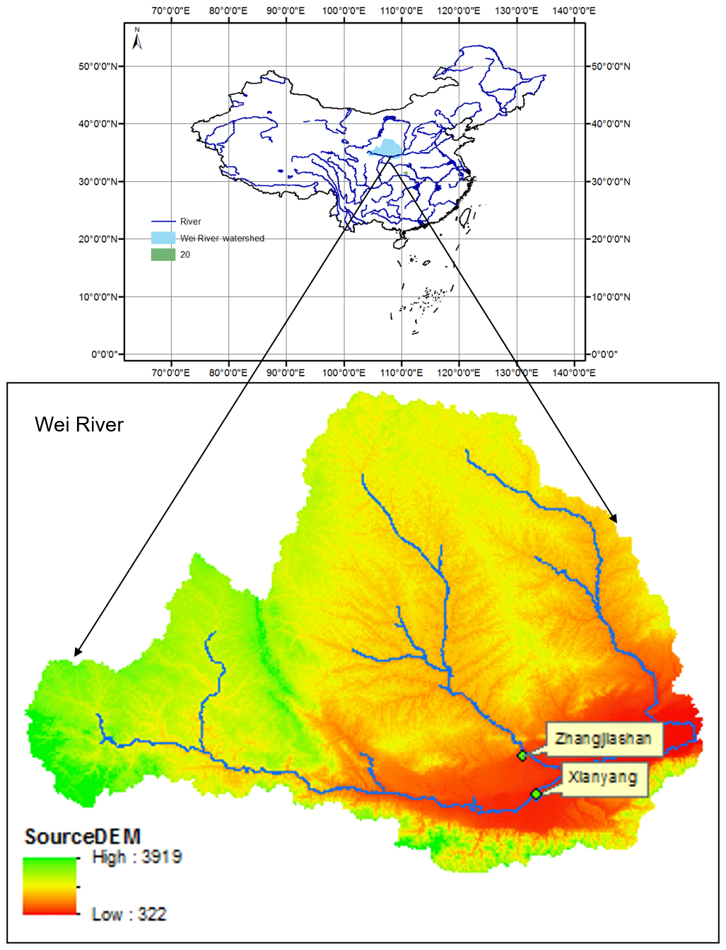
Figure 2The location of the studied watersheds. The Wei River is the largest tributary of the Yellow River, with a drainage area of 135 000 km2. The historical flood data from the Xianyang and Zhangjiashan stations on the Wei River are analysed through the proposed IFC approach.
4.1 Model evaluation and selection
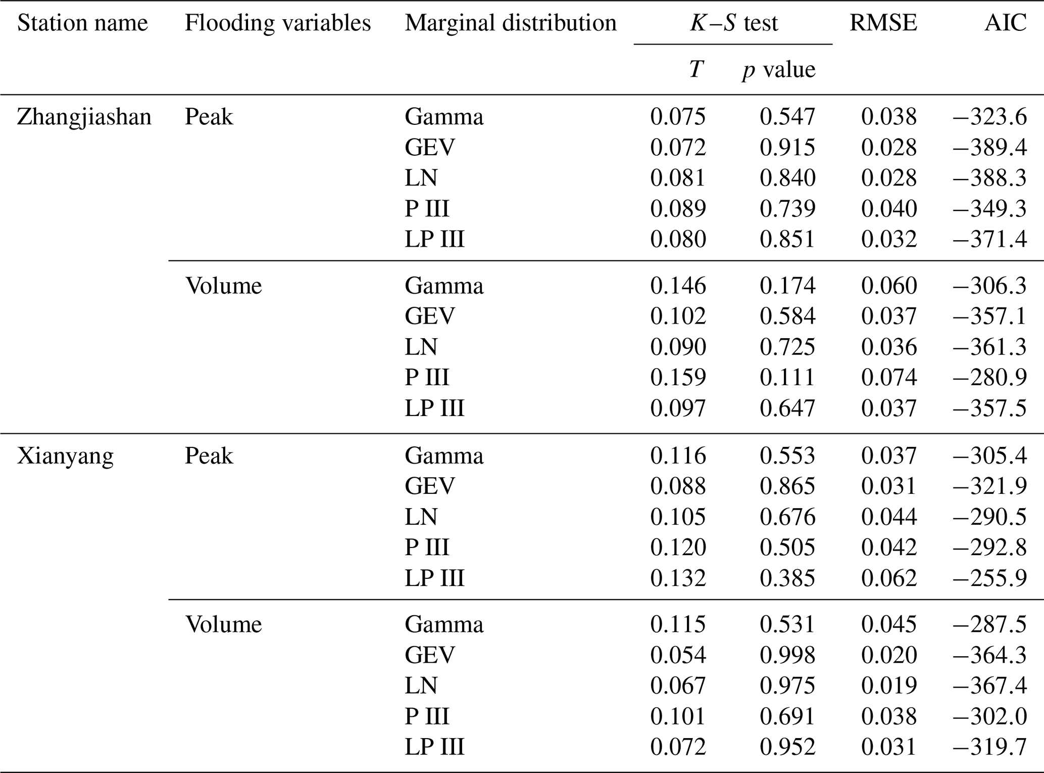
There are a number of potential probabilistic models for modelling individual flood variables and their dependence structures. In this study, five alternative distributions, including gamma, generalized extreme value (GEV), lognormal (LN), Pearson type III (P III), and log-Pearson type III (LP III) distributions, are employed to describe the probabilistic features of the chosen flood variables (i.e. peak and volume). Moreover, goodness-of-fit tests are performed through the indices of Kolmogorov–Smirnov test (K–S test), root mean square error (RMSE), and Akaike information criterion (AIC) to screen the performance of those potential models. The results are presented in Table 2. The results indicate that all five parametric distributions can produce satisfactory results, with all p values larger than 0.05. However, it can be concluded that the GEV and lognormal approaches show the best performance for, respectively, modelling flood peak and volume at both gauging stations.
Table 2Statistical test results for marginal distribution estimation: LN means lognormal distribution, P III means Pearson type III distribution, and LP III means log-Pearson type III distribution. K–S test denotes the Kolmogorov–Smirnov test.
In addition, a total number of six copulas, including Gaussian, Student's t, Clayton, Gumbel, Frank, and Joe copulas, are considered as the candidate models for quantifying the dependence structures for flood peak volume at the Xianyang and Zhangjiashan gauging stations. Also, the goodness-of-fit statistic test is performed based on the Cramér–von Mises statistic proposed by Genest et al. (2009). The indices of RMSE and AIC were employed to evaluate the performance of the obtained copulas and identify the most appropriate ones. Table 3 shows statistical test results for the selected copulas. The results show that, for the Zhangjiashan station, all candidate copulas except the Joe copula performed well, while all six copulas would be able to provide satisfactory risk inferences at the Xianyang station. Moreover, based on the values of RMSE and AIC, the Gumbel copula was chosen to model the dependence of flood peak and volume at the Zhangjiashan station, while the Joe copula performed best at the Xianyang station, except that although the p value is slightly lower than Gumbel, the overall result favours Joe. Consequently, the Gumbel and Joe copulas were chosen in this study to further characterize the uncertainty in model parameters and the resulting risks at the Zhangjiashan and Xianyang stations, respectively.
Table 3Performance for quantifying the joint distributions between flood peak and volume through different copulas: CvM is the Cramér–von Mises statistic proposed by Genest et al. (2009), with a p value larger than 0.05 indicating satisfactory performance.


Figure 3Probabilistic features for parameters in marginal distributions and copula: for both the Xianyang and Zhangjiashan stations, the GEV (parameters include shape, scale, and location) function would be employed to quantify the distribution of flood peak, while the lognormal distribution (parameters denoted as meanlog and sdlog) is applied for flood volume. The Gumbel and Joe copulas (parameter denoted as theta) would be, respectively, adopted to model the dependence between flood peak and volume at the Zhangjiashan and Xianyang stations.
4.2 Uncertainty in model parameters and risk inferences
Based on the results in Tables 2 and 3, the multivariate risk inference model was established, in which the GEV and lognormal distributions would, respectively, be adopted to model the individual flood variables at both gauging stations, while in comparison, the Gumbel and Joe copulas would, respectively, be employed for the Zhangjiashan and Xianyang stations. Afterward, uncertainties would be characterized based on the bootstrap algorithm illustrated in Sect. 2.2. In this study, a total number of 5000 samples was chosen in order to generally visualize the uncertainty features in the model parameters. The probabilistic features for obtained parameter values (i.e. shape, scale, and location for GEV, meanlog, sdlog for LN, and theta for copula) for each sample scenario would be described by the kernel method. Figure 3 exhibits the probabilistic distributions for the six unknown parameters in the established multivariate risk inference model. Extensive uncertainties exist in the parameters for both the marginal distribution and dependence model. As presented in Fig. 3, each parameter, except the meanlog in the LN distribution, exhibits noticeable uncertainty. Moreover, most of the parameter uncertainties are approximately normally distributed, except the shape parameter in GEV for Xianyang.
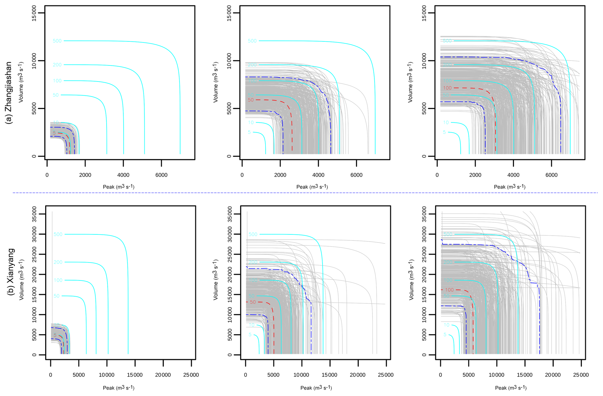
Figure 4Uncertainty quantification of the joint RP in “AND”: the red dash lines indicate the predictive means, the two blue dash lines, respectively, indicate the 5 % and 95 % quantiles, and the grey lines indicate the predictions under different parameter samples with the same joint RP of the red and blue dash lines. The cyan lines denote the predictions under different return periods, with the model parameters being their mean values.
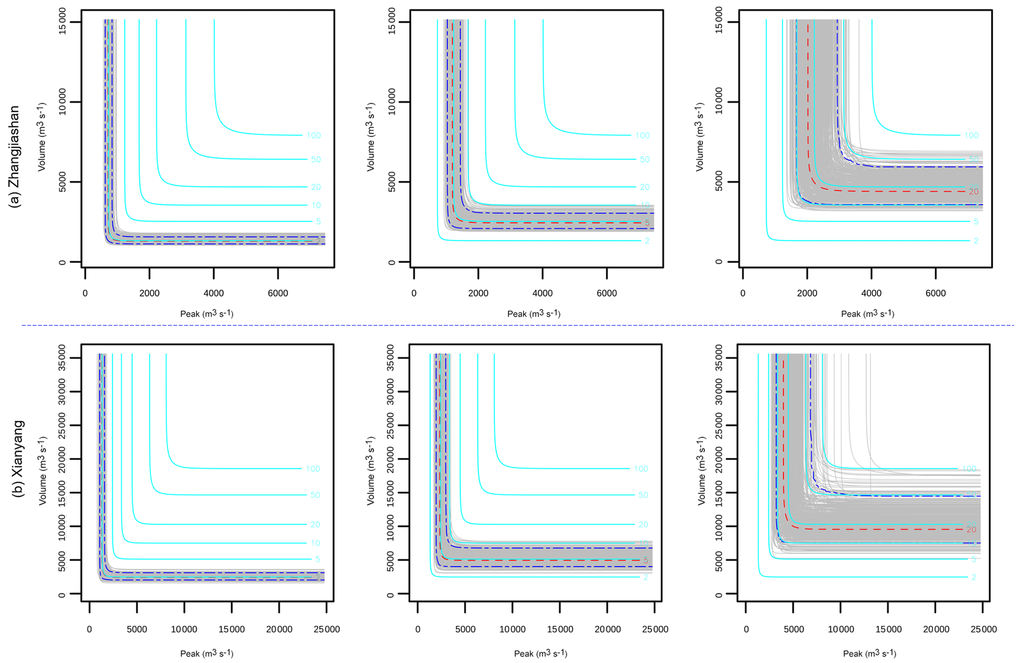
Figure 5Uncertainty quantification of the joint RP in “OR”: the red dash lines indicate the predictive means, the two blue dash lines, respectively, indicate the 5 % and 95 % quantiles, and the grey lines indicate the predictions under different parameter samples with the same joint RP of the red and blue dash lines. The cyan lines denote the predictions under different return periods, with the model parameters being their mean values.

Figure 6Uncertainty quantification of the joint RP in “Kendall”: the red dash lines indicate the predictive means, the two blue dash lines, respectively, indicate the 5 % and 95 % quantiles, and the grey lines indicate the predictions under different parameter samples with the same joint RP of the red and blue dash lines. The cyan lines denote the predictions under different return periods, with the model parameters being their mean values.
It is quite apparent that different parameter values in the copula model would lead to different risk inference results. Consequently, parameter uncertainties in the marginal distributions and copula functions would definitely result in uncertainties in multivariate risk inferences. Based on the copula model, some multivariate risk indices can be easily obtained, such as the joint return period in OR, AND, and Kendall, as expressed in Eqs. (11a)–(11c). However, due to parameter uncertainties, these risk indices may also exhibit some degrees of uncertainty. Figures 4–6 describe uncertainties for the joint RP in AND, OR, and Kendall at the two stations. In general, the predictive RP in AND exhibit most significant uncertainty, followed by the predictive RP in OR and Kendall. However, for moderate or large flood events, considerable uncertainties can be observed in the inferences for all three joint RPs. Specifically, noticeable uncertainties exist in the predictive joint RP of AND even for a minor flood event with a 5-year joint RP. For some large flood events with a joint RP around 100 years, the predictive RP in AND shows remarkable uncertainty, ranging from less than 50 years to larger than 200 years. For the joint RP in OR and Kendall, slight uncertainty may exist for small flood events (e.g. 2- or 5-year joint RP). Nevertheless, apparent uncertainties can be observed in the predictive joint RP even for moderate flood events. As shown in Fig. 5, considerable uncertainties may appear in the predictive joint RP of OR even for a flood with an actual joint RP of 20 years, while prediction of the Kendall RP for a 20-year (in Kendall RP) flood event may range from 10 to 50 years, as presented in Fig. 6.
4.3 Individual and interactive effects of parameter uncertainties
It has been observed that parameter uncertainties in the copula-based multivariate risk model would lead to significantly imprecise risk predictions. However, one critical issue to be addressed is how the parameter uncertainties and their interactions would influence the risk inference. Consequently, a multilevel factorial analysis, based on Eqs. (12) and (13), was proposed to primarily visualize the individual and interactive effects of parameter uncertainties in the marginal and dependence models on the resulting risk inferences. In this study, a total number of six parameters (i.e. three from GEV, two from LN, and one from copula) was addressed, and based on probabilistic features of these parameters, three quantile levels (i.e. 0.1, 0.5, and 0.9) were chosen to characterize the resulting risk inferences under different parameter values. This would finally form a 36 factorial design, which has six factors, with each having three levels. The failure probability denoted as Eq. (10) would be considered the response in this factorial design.
Table 4ANOVA table for failure probability in AND: A indicates the shape parameter in GEV, B indicates the scale parameter of GEV, C indicates the location parameter of GEV, D means the meanlog of LN, E means the sdlog of LN, and F means the parameter (i.e. theta) in copula.

The main and interactive effects of parameter uncertainties on the failure probabilities in AND are visualized in Fig. 7. It is noticeable that at the two gauge stations, parameter uncertainties have similar main and interactive effects on the failure probabilities in AND, which indicates that parameters' effects (individual and interactive) on the failure probability in AND are independent of the location of gauge stations. More specifically, variations in the shape parameter in GEV and sdlog parameter in LN would lead to more changes in the corresponding responses (i.e. failure probability in AND) than the variations in other parameters. Also, as shown in Fig. 7, the parameter in the copula function (i.e. Cop_theta), describing dependence of the two flood variables, would not have an effect on the resulting risk as much as the effects from the parameters (except the location parameter in GEV) in the marginal distributions. In terms of parameter interactions, the significance of interactive effects for different parameters varies. The interactive curves for some parameters (e.g. GEV_shape and GEV_location) are nearly parallel at the three levels, indicating an insignificant interaction for these two parameters on the inferred risk. In comparison, there are also some interactive curves intersecting each other (e.g. GEV_shape and LN_meanlog), implying a significant interaction between these two parameters. Table 4 provides the results from an ANOVA table for the failure probability in AND. It is quite interesting that (i) even though the effect from the parameter in the copula function is not as visible as the effects from the parameters (except the location parameter in GEV) in the marginal distributions (as shown in Fig. 7), such an effect is still statistically significant; (ii) the effect from the location parameter of GEV is statistically insignificant, which also leads to insignificant interactive effects between the location parameter and other parameters; (iii) the interactions between the parameter in copulas and the parameters in marginal distributions would be more likely statistically insignificant; (iv) the statistical significance (significant or not) for individual and interactive effects from parameters is almost the same between these two gauge stations. All these conclusions obtained from Table 4 are consistent with the implications described in Fig. 7.
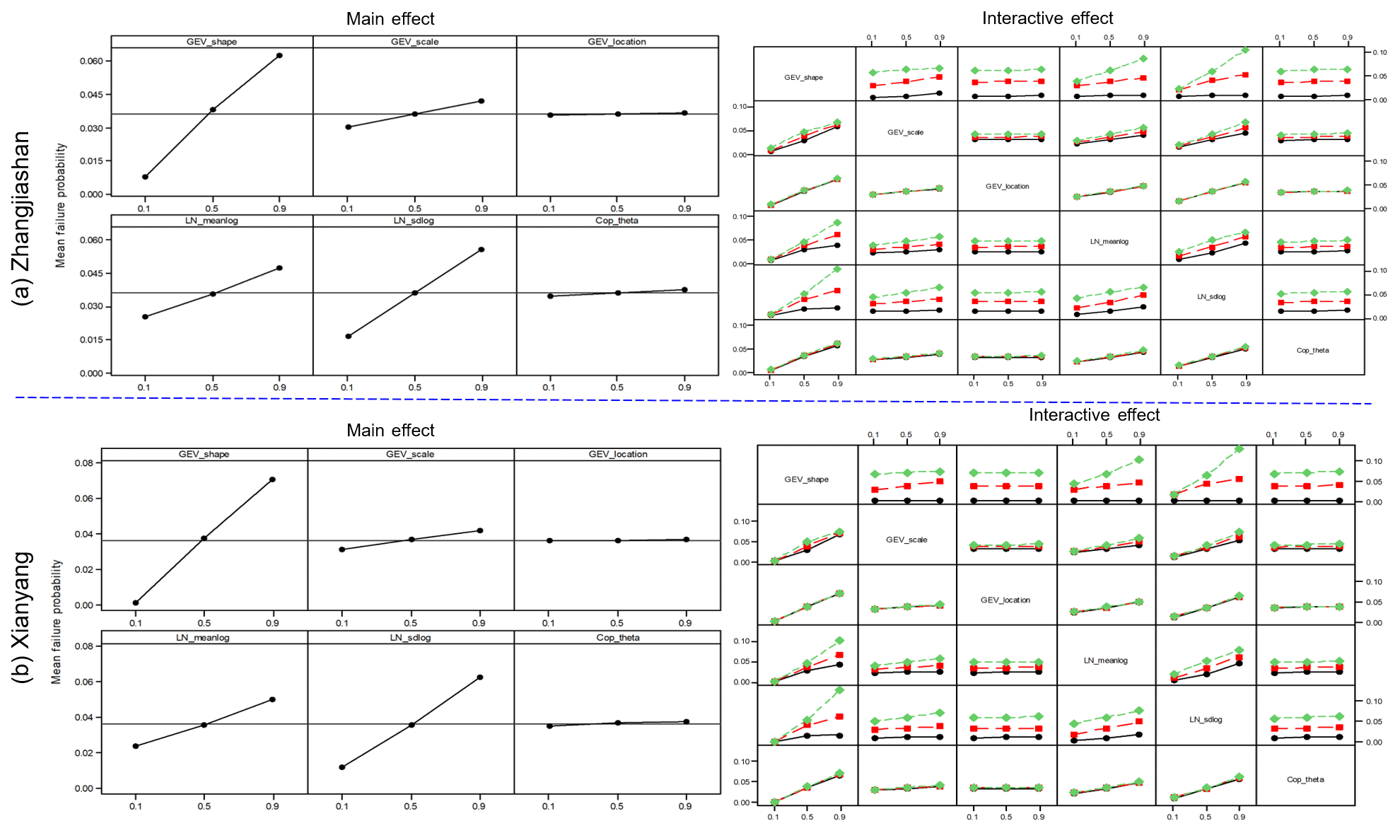
Figure 7Main effects plot and full interactions plot matrix for parameters on the failure probability in AND at the two gauge stations.
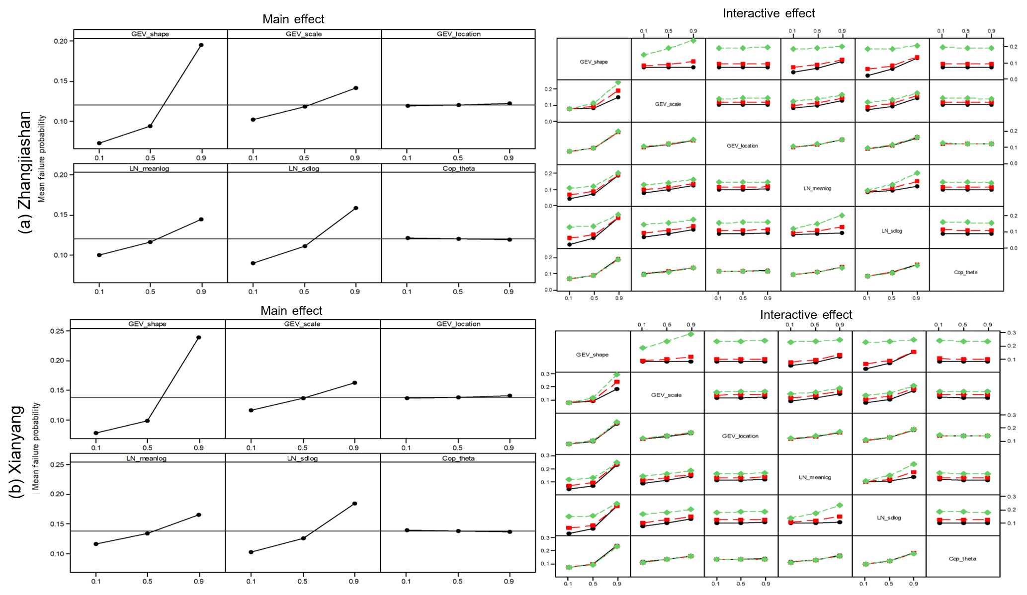
Figure 8Main effects plot and full interactions plot matrix for parameters on the failure probability in OR at the two gauge stations.
In terms of the failure probabilities in OR and Kendall, as presented in Figs. 8 and 9, these have similar patterns to the failure probability in AND (presented in Fig. 7). The individual/main effects from the marginal distributions (except the location parameter in GEV) are generally more visible than the parameters in copula functions. Also, some interactive curves, especially the curves between GEV_location and others, are parallel, showing insignificant interaction between those parameters. More detailed characterizations of the main and interactive effects for the failure probabilities in OR and Kendall are described in the ANOVA tables in Tables 5 and 6. These two tables show some slight differences from the conclusions given by Table 4. The location parameter in GEV also has a statistically significant effect on the failure probabilities results in OR and Kendall, which also leads to some significant interactions between this parameter and other model parameters. For the failure probability in Kendall, the parameter in the copula would have more interactions with other parameters in marginal distributions than the interactions in the failure probability in AND and OR. As presented in Table 6, the parameter in the copula would have a statistically significant effect on the inferred failure probability in Kendall with other parameters except the location parameter in GEV. These results are also implied in the main effects plots and full interactions plot matrices in Figs. 8 and 9.
Table 5ANOVA table for failure probability in OR: A indicates the shape parameter in GEV, B indicates the scale parameter of GEV, C indicates the location parameter of GEV, D means the meanlog of LN, E means the sdlog of LN, and F means the parameter (i.e. theta) in copula.
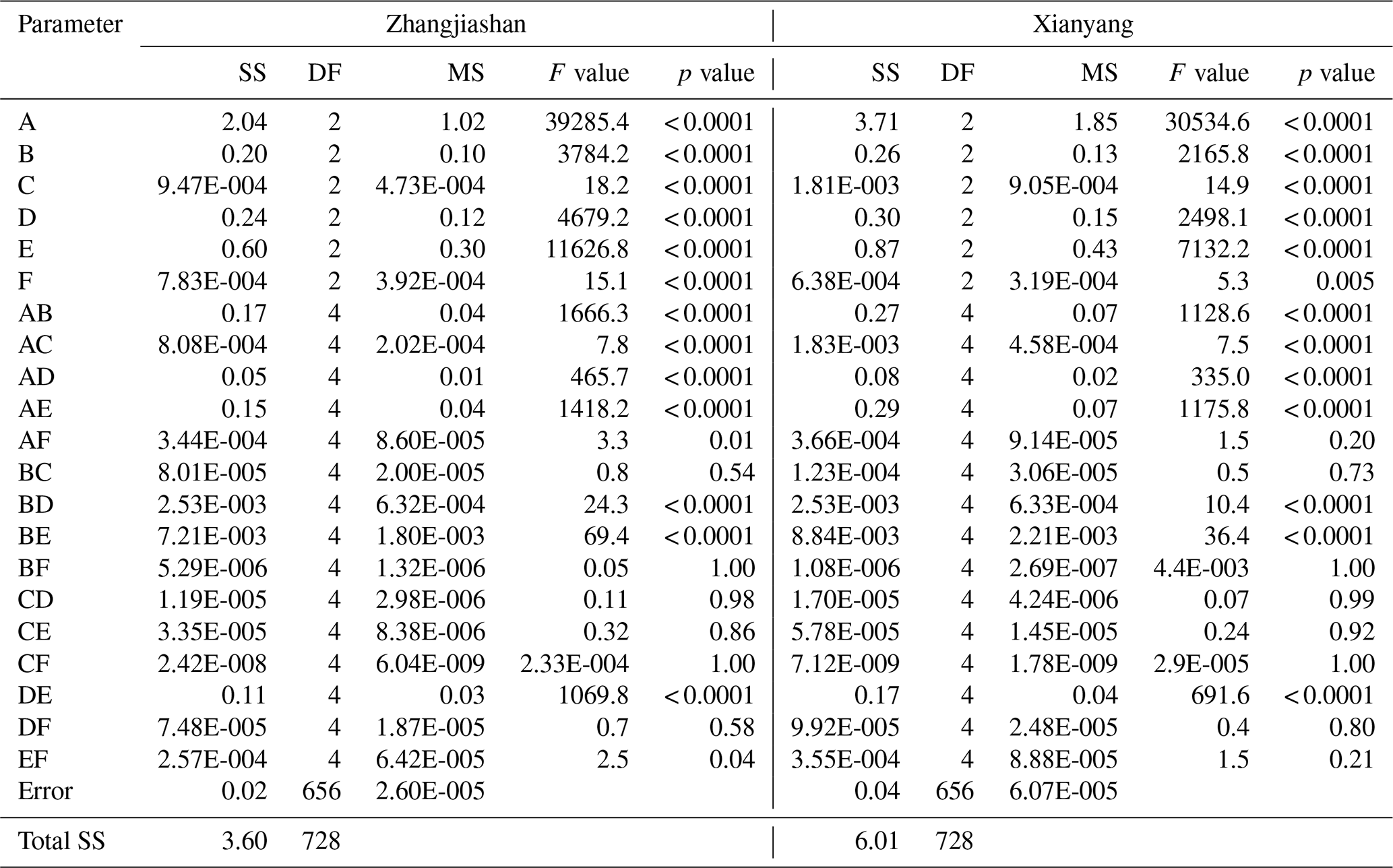
Table 6ANOVA table for failure probability in Kendall: A indicates the shape parameter in GEV, B indicates the scale parameter of GEV, C indicates the location parameter of GEV, D means the meanlog of LN, E means the sdlog of LN, and F means the parameter (i.e. theta) in copula.

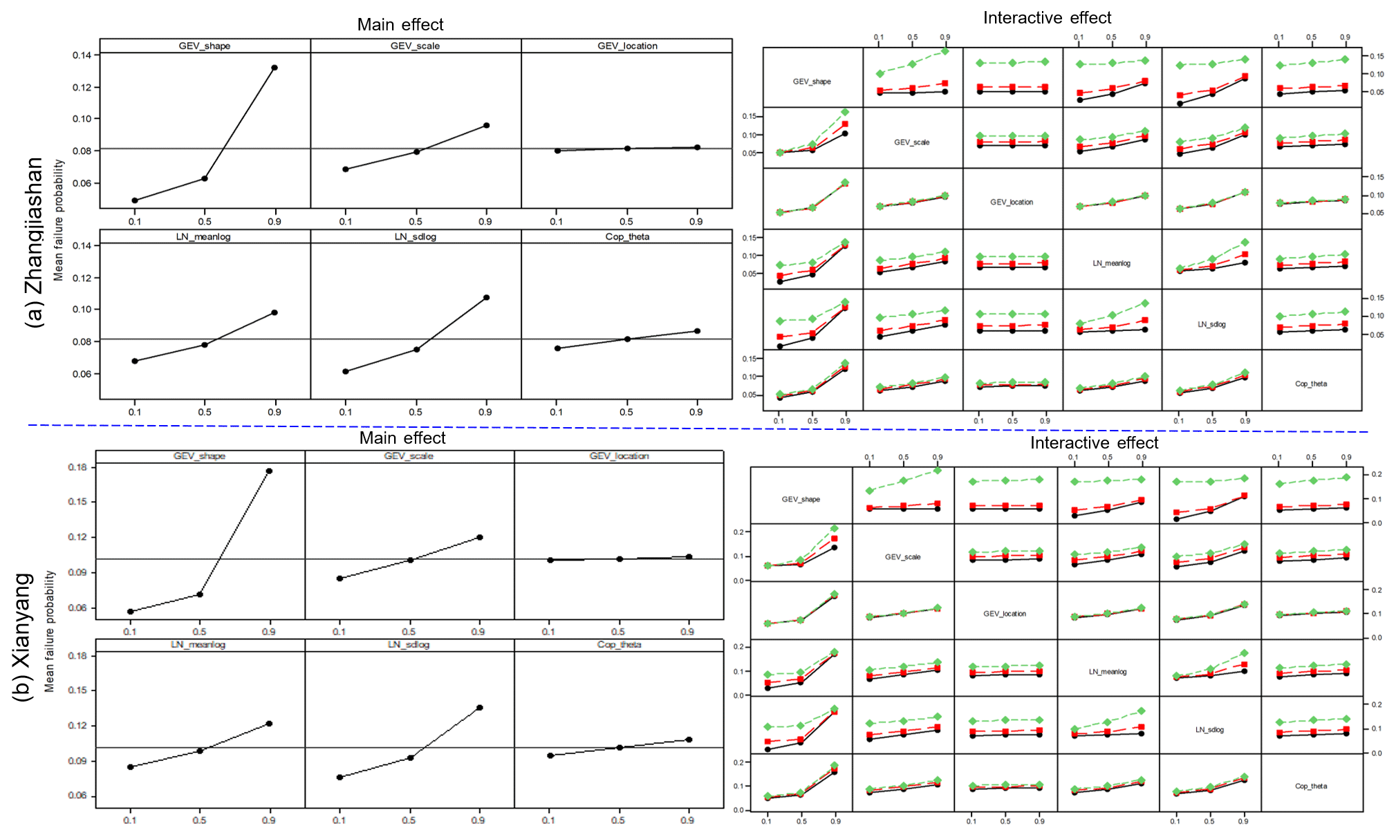
Figure 9Main effects plot and full interactions plot matrix for parameters on the failure probability in Kendall at the two gauge stations.
Based on the three-level factorial analysis, it can be generally concluded that the parameters in the marginal distributions (except the location parameter in GEV) would have more individual effects on joint risk inference than the parameter in the copula. The risk indices (i.e. AND, OR, or Kendall) would not have significantly influenced the individual effects of model parameters. However, for the interactive effects among model parameters, they may exhibit slightly different patterns. Specifically, the parameter in the copula would have more significant interactions with parameters in the marginal distributions on the failure risk in Kendall than the other two risk indices. Moreover, the individual and interactive effects from the model parameters on risk inferences would not be influenced by the location of the gauge stations.
4.4 Contribution partition of uncertainty sources
As a result of parameter uncertainties, the predictive failure probabilities exhibit noticeable uncertainties, as shown in Figs. 4–6. The three-level factorial analysis based on Eq. (13) is able to provide a primary description and visualization related to the individual and interactive effects of parameter uncertainty on the inferred failure probabilities. However, two critical issues to be answered are (i) how much would parameter uncertainties contribute to the variation of the inferred risk values and (ii) do these contributions change significantly for failure probabilities with different service time scenarios? To address these two issues and get reliable results, an iterative factorial approach (IFA) has been proposed, which is formulated as Eqs. (15)–(19). Also, like the three-level factorial analysis, three quantile levels were selected at 0.1, 0.5, and 0.9. Based on IFA, each parameter at its three quantile values (0.1, 0.5, 0.9) would be further subsampled into three scenarios of two quantile values (i.e. (0.1, 0.5), (0.1, 0.9), and (0.5, 0.9)). For this study, we have a total number of six parameters, with each having three quantile values at 0.1, 0.5, and 0.9, which would lead to a total number of 729 (i.e. 36) two-level factorial designs.
Table 7Contributions of parameter uncertainties to predictive failure probabilities in AND under different design standards (i.e. return periods – RPs) and different service periods.
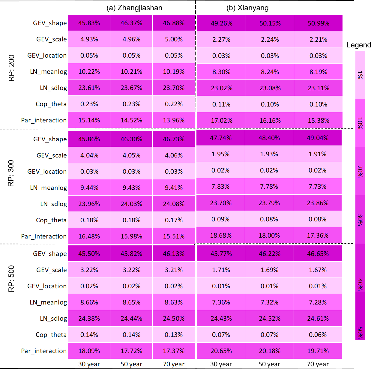
Table 7 shows the detailed contribution table of the model parameters on uncertainty in predictive failure probabilities of AND at the two gauge stations. It can be observed that, even though some discrepancies exist at the Zhangjiashan and Xingshan stations, the detailed contributions for each parameter and their interaction show quite similar features between these two stations. In detail, uncertainty in the shape parameter in GEV has the most significant impact on the failure probability in AND, followed by sdlog in LN, parameter interaction, meanlog in LN, and scale parameter in GEV. Moreover, the uncertainty in the parameter in the copula would not lead to a significant variation in the resulting failure probability predictions in AND, which merely makes a contribution less than 0.5 %. Such conclusions are also generally consistent with the ANOVA results presented in Fig. 7 and Table 4. Furthermore, with the increase in service time, the contributions of each parameter and their interactions do not vary significantly. Some individual contributions from parameter uncertainties would slightly increase, while other individual contributions may slightly decrease. However, the effect from parameter interactions would generally increase with the increase in service time. In comparison, the enhancement in design standards for hydraulic infrastructures would lead to a greater chance of deceases in individual effects and, at the same time, increases in parameter interactions. For instance, as the flood design standard increases from 200 to 500 years for a hydraulic facility with 30-year service time near the Zhangjishan station, the interactive effect of model parameters would increase from 15.14 % to 18.09 %.
Table 8Contributions of parameter uncertainties to predictive failure probabilities in OR under different design standards (i.e. return periods – RPs) and different service periods.
In terms of the failure probability in OR, the individual and interactive effects of model parameters on predictive risk uncertainties show similar patterns with the parameters' effects on the failure probability in AND. As shown in Table 8, the shape parameter in the GEV distribution and the sdlog in the LN distribution are the two major sources of uncertainty in failure probabilities in OR. However, compared with the failure probability in AND, parameter interaction has a less effect on the resulting uncertainty of risk inference in OR. As shown in Tables 7 and 8, the effect of parameter interaction on the risk in AND ranges between 13.96 % and 20.05 %, while in comparison, the parameters' interactive effect on the risk in OR varies between 10.25 % and 11.57 %. Apparently, it can also be observed that some external factors such as the design standard and service time of hydraulic infrastructures have less influence on the parameters' interaction on risk in OR than the risk in AND. However, the first contributor (i.e. shape parameter in GEV) would have a larger contribution on the predictive uncertainty in the failure probability in OR as the increase in the design standard, while in comparison, this contributor would have a lower contribution on the risk in AND. For instance, as the design return period of flood (i.e. design standard) increases from 200 to 500 years and the service time of the hydraulic facility is 30 years, the contribution of the shape parameter in GEV would increase from 47.62 % to 50.64 % for the failure probability in OR at the Xianyang station, while the parameter's contribution on the failure probability in AND decreases from 49.26 % to 45.77 %.

Figure 10Variation of parameters' contributions for different risk inferences at the Zhangjiashan station for a design standard of 200 years and a service time of 30 years.
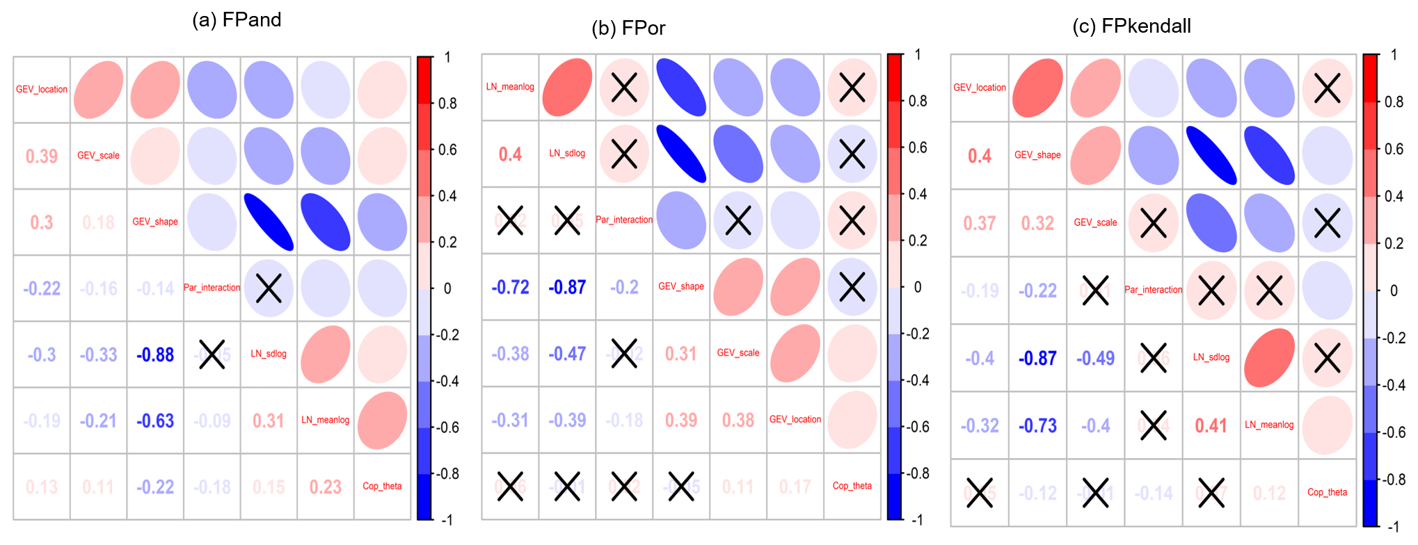
Figure 11Correlation for parameters' contributions to risk inferences at the Zhangjiashan station for a design standard of 200 years and a service time of 30 years: the cross sign indicates the correlation is statistically insignificant.
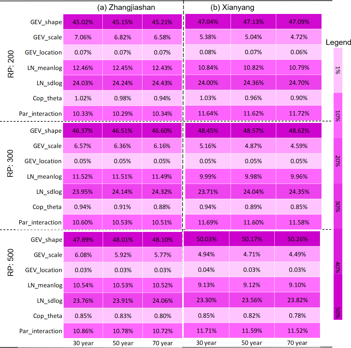
Table 9Contributions of parameter uncertainties to predictive failure probabilities in Kendall under different design standards (i.e. return periods – RPs) and different service periods.

For the failure probability in Kendall, the contributions of model parameters and their interaction are presented in Table 9. Similar to the failure probabilities in AND and OR, the shape parameter in the GEV distribution and the sdlog parameter in the LN distribution are the two major contributors, which can account for nearly 70 % or more in the predictive uncertainty of the failure probability in Kendall. Meanwhile, the scale parameter in GEV, meanlog in LN, and parameters' interaction also have noticeable effects on the risk in Kendall, ranging from 4.72 % (scale parameter in GEV) to 12.64 % (meanlog in LN). Conversely, the location parameter in GEV and the dependence parameter in copula merely have relatively minor individual effects. However, it is noticeable that, although the dependence parameter has a minor effect (0.78 %, 1.03 %) on the risk in Kendall, such an effect is much higher than the effect on the risk in AND (less than 0.23 %) and the risk in OR (less than 0.06 %).
Even though the prediction equations for the failure probabilities in AND, OR, and Kendall as presented in Eq. (11) are different, the impacts of parameter uncertainties show quite similar features, in which the shape parameter in GEV and the sdlog in LN are the two major contributors to the predictive uncertainties in risk inferences. Nearly 70 % and more variability in the uncertainties in risk inferences can be attributed by the uncertainties in the shape parameter in GEV and sdlog parameter in LN. Also, some external factors such as flood design and facility service time may have different influences on parameters' effects for different risk indices; such influences are not significant and would not lead to remarkable changes in parameters' contributions to risk inferences. Parameters' interaction has a greater effect on risk inference in AND than the other two risk indices (i.e. OR, Kendall), while the contribution from the dependence parameter, even though not noteworthy, has a larger effect on the risk inference in Kendall.
5.1 Differences for the hydrologic risk models at different stations
Different copula functions are applied for different stations, which are chosen based on the indices of RMSE and AIC. However, the selection of copula models at different stations may also be related to some key characteristics of the drainage areas for those stations. The Gumbel copula will be applied for the Zhangjiashan station. It can reflect strong correlation at high values. However, the Joe copula, which is adopted at the Xianyang station, can reflect a stronger right-tail positive dependence than the Gumbel copula. Both the Xianyang and Zhangjiashan stations have similar drainage areas. The Xianyang station controls a drainage area of 46 480 km2 (Xu et al., 2016), while the Zhangjiashan station has a drainage area of 45 412 km2 (Sun et al., 2019). Nevertheless, the major reason that led to different copula functions at these two stations may be the elevation features for those two drainage areas. The drainage area of the Zhangjiashan station is located in the central part of the Loess Plateau of China, which is mainly characterized as a mountainous region. In comparison, even though a large part of the drainage area of the Xianyang station is also located in the mountainous region, the Xianyang station also controls a large part of the Guanzhong Plain, as indicated in the red part of Fig. 2. Consequently, the flood hydrograph at the Zhangjiashan station may be sharp, while the flood hydrograph at the Xianyang station is relatively flat and shows a stronger right-tail dependence among flood peak and volume. In fact, the value of Kendall's tau between peak and volume for the top 10 floods at the Zhangjiashan station is 0.33, while such a value of Kendall's tau at the Xianyang station is 0.6. These facts may explain why the Gumbel copula is applicable for the Zhangjiashan station while the Joe copula is applied for the Xianyang station. However, this is an initial guess and may need to be further demonstrated through more cases in different areas.
5.2 Contribution partition of uncertainty sources through different approaches
In this study, the individual and interactive contributions of parameter uncertainties are quantified through the developed IFA approach, in which each parameter has three levels (i.e. 0.1, 0.5, and 0.9 quantiles) to be subsampled. In fact, the parameters' contributions can also be characterized by the traditional factorial analysis (FA) approach based on Eq. (14) as well as the IFA approach with more factor levels (e.g. four or five levels for each parameter).
Table 10Comparison of parameter contributions to predictive uncertainty for failure probabilities under different levels of subsampling for the Zhangjiashan station: three (i.e. 0.1, 0.5, 0.9) and four (i.e. 0.1, 0.35, 0.6, 0.85) level quantiles are adopted for subsampling and the design return period is 200 years.
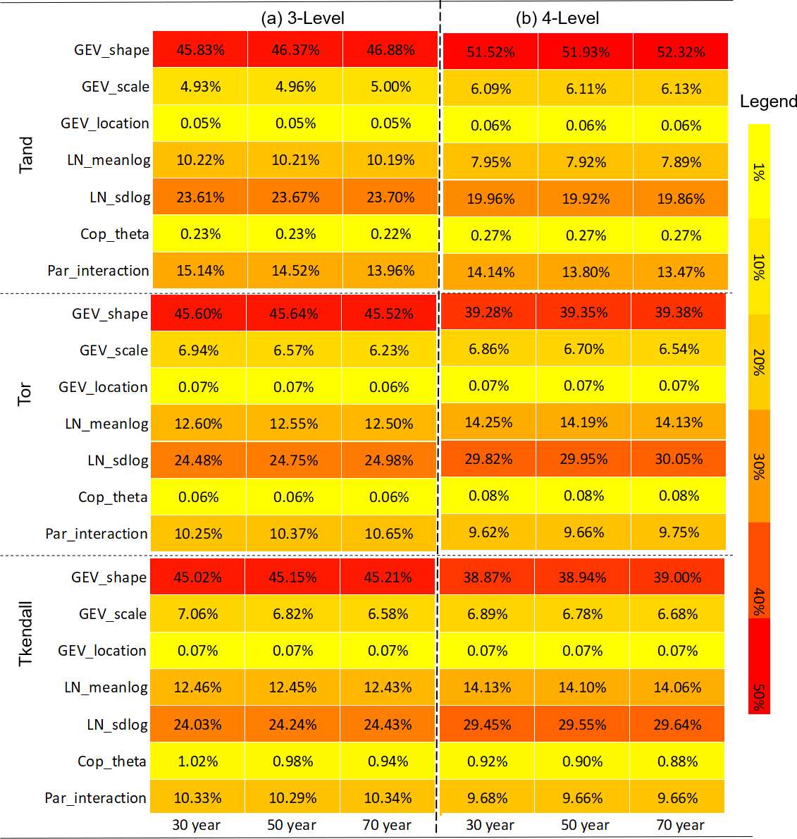
Table 10 shows the comparison of parameter contributions to predictive uncertainty for failure probabilities in AND at the Zhangjiashan station for three and four parameter level scenarios for the design standard of 200 years. The results of Table 10b are obtained through the IFA approach, with each parameter having four levels to be its quantiles at 0.1, 0.35, 0.6, and 0.85. Also, Table 11 presents the parameter contributions to predictive uncertainty in failure probabilities obtained by the traditional FA approach for the Zhangjiashan station with the design standard of 200 years and service time of 30 years.
Table 11Contributions of parameter uncertainties obtained by three-level ANOVA to predictive failure probabilities for a design return period of 200 years and a service time of 30 years.
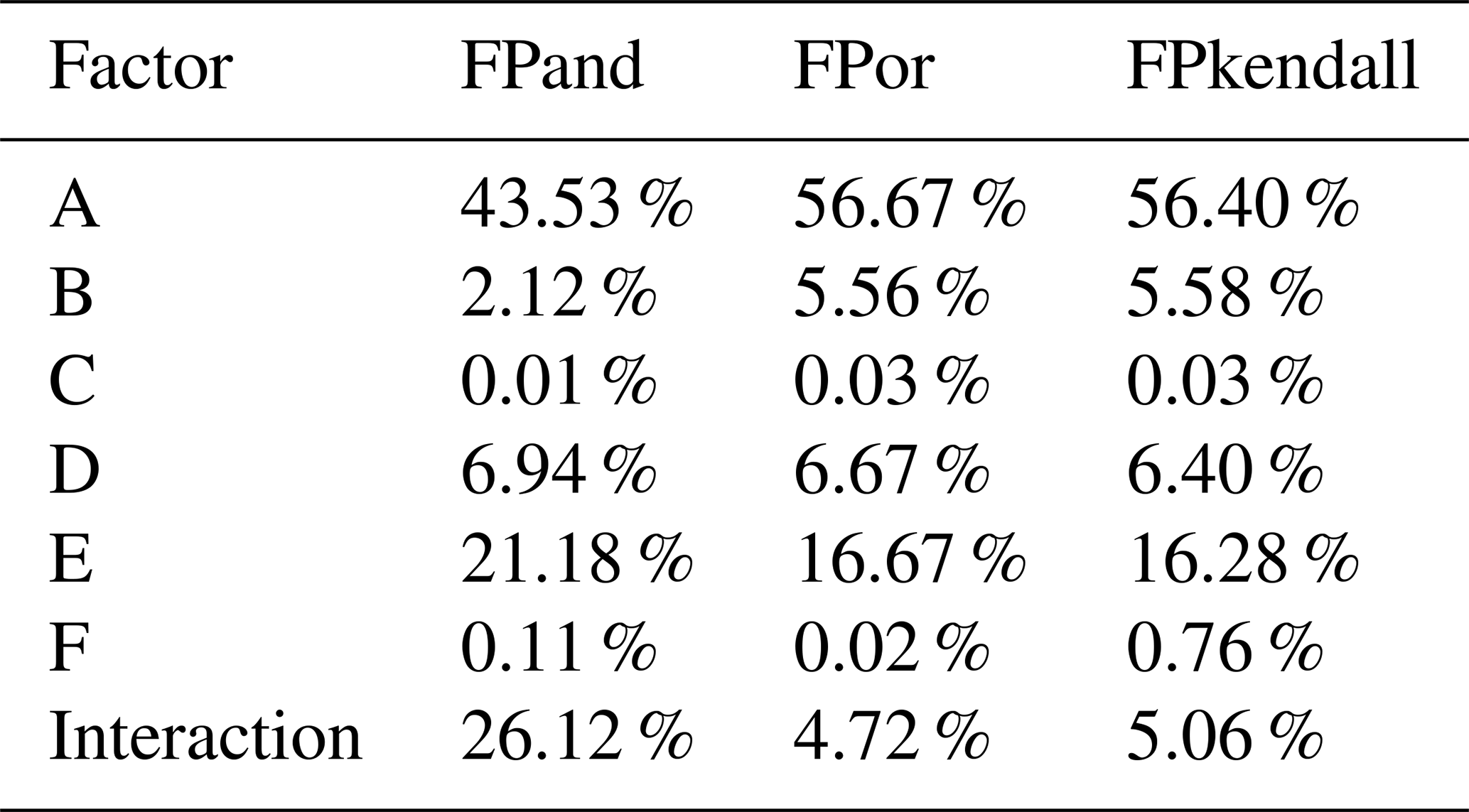
It can be seen that for different subsampling scenarios, the resulting contributions may be different. However, such a difference would be tolerable since (1) the variations of parameters' contributions are relatively small and mainly happen for the first two contributors, (2) the total contribution of the first two contributors does not change remarkably (around 70 % in total), (3) the contributions of other factors, especially the parameters' interaction, do not vary significantly, and (4) the rank of the contributions from different sources does not change for the two subsampling scenarios. In comparison, as presented in Table 7, the contribution partition of parameter uncertainties obtained through traditional FA shows totally different patterns for different risk inferences. Specifically, the traditional FA approach would significantly overestimate parameter interactive effects on risk inference in AND; at the same time, it would underestimate the interactive effects on risk inference in OR and Kendall. Consequently, the contribution rank of parameter uncertainties from traditional FA is different from the results obtained through the developed IFA approach.
As shown in Table 10, the proposed IFA approach may lead to slightly different results for different subsampling schemes (four or five levels). However, an increase in parameter level would highly increase computational demand. For instance, if each parameter has four levels, the IFA approach would lead to a total number of 46 656 (i.e. 66) two-level factorial designs. Moreover, the subsampling scheme for factors with five levels would lead to a total number of 1 million (i.e. 106) two-level factorial designs. Consequently, the three-level subsampling scheme would generally be recommended and also can generate acceptable results.
5.3 Correlation among parameter contributions
The proposed IFA approach would generally produce a great number of two-level factorial designs. For one specific factor (e.g. GEV_shape), it would have two levels (lower and upper levels) for all factorial designs. However, the detailed value for the lower or upper level may be different in different factorial designs. This may finally lead to different contributions for this factor. Figure 10 presents the variations of parameters' contributions to the prediction of failure probabilities in AND, OR, and Kendall. We already concluded that the shape parameter in GEV (i.e. GEV_shape) and the sdlog in LN (i.e. LN_sdlog) distribution would generally have the most significant contributions to predictive uncertainties in risk inferences. However, as shown in Fig. 10, the detailed contributions for these two parameters would vary remarkably for different level values in different factorial designs. In comparison, the contributions from other parameters and their interaction have less fluctuation than the individual contributions of GEV_shape and LN_sdlog. For instance, although the meanlog in LN (i.e. LN_meanlog), with an average contribution of more than 10 %, may have some chance to pose a predominant contribution of more than 50 %, most of its contribution is positively distributed within [0 %, 25 %]. Also, even though the parameters' interaction has a noteworthy average contribution larger than 10 %, all the detailed contributions in different factorial designs are located within [0 %, 25 %].
It has been observed that the parameters' contributions may vary significantly due to the differences in factor values in different factorial designs. One potential issue to be addressed is how those individual and interactive contributions correlate with each other. Figure 11 presents Pearson's correlation among individual and interactive contributions of model parameters to different risk inferences (i.e. failure probabilities in AND, OR, and Kendall). It is noticeable that the parameters in the LN distribution (i.e. LN_sdlog, LN_meanlog) are generally negatively correlated with the parameters in the GEV distribution (i.e. GEV_shape, GEV_scale, and GEV_location). Also, for one marginal distribution (LN or GEV), its parameters are positively correlated. This implies that an increase in the contribution of one parameter would lead to a contribution increase for parameters within the same distribution and at the same time result in a contribution decrease for all parameters in the other distribution. Moreover, if statistically significant, the contribution of the dependent parameter (i.e. parameter in copula) generally has positive correlation with the contributions from other parameters except GEV_shape and parameters' interaction. Also, the contributions from parameters' interactions are generally negatively correlated with the individual contributions from other parameters if such a correlation is statistically significant.
The proposed IFA approach can generally characterize how parameter uncertainties would influence the predictive uncertainties in risk inferences. A large number of two-level factorial designs was produced due to different subsampling procedures and then used to generate different partition results for parameters' contributions. However, for different risk inferences (i.e. failure probabilities in AND, OR, and Kendall), these partition results have similar variation features and also show similar correlation plots.
Uncertainty quantification is an essential issue for both univariate and multivariate hydrological risk analyses. A number of research works have been posed to reveal uncertain features in multivariate hydrological risk inference. However, it is required to know the major sources/contributors for predictive uncertainties in multivariate risk inferences. In this study, an iterative factorial copula approach (IFC) has been proposed for uncertainty quantification and partition in multivariate hydrologic risk inference. In IFC, a copula-based multivariate risk model has been developed, and the bootstrap method is adopted to quantify the probabilistic features for the parameters in both marginal distributions and the dependence model. An iterative factorial analysis (IFA) approach was finally developed to diminish the effect of the sample size in traditional ANOVA computation and provided reliable contribution partition for parameter uncertainties in different risk inferences.
The proposed method has been applied for flood risk inferences at two gauge stations in the Wei River basin. The results indicate that uncertainties in the parameters of the copula-based model would lead to noticeable uncertainties in the resulting risk inferences, especially for the joint flood risk in AND. Noticeable uncertainties exist in the predictive joint RP of AND even for a small flood event. However, the results from IFA suggested that those uncertainties in risk inferences may mainly be attributed to the uncertainties in the shape parameter in the GEV distribution and the parameter of sdlog in LN for both the two stations. In comparison, the parameter uncertainty in the copula function would not have an obvious effect on the resulting uncertainty in risk inferences. Such results indicate that, at least for the Wei River basin, the decision makers need to estimate the values or quantify the uncertainties well for the shape parameter in the GEV distribution and sdlog in the LN distribution, in order to obtain reliable risk inferences. For other catchments, the proposed IFC method can be adopted to reveal the major sources for uncertainties in risk inferences and then provide potential pathways to get reliable risk inferences.
This study is the first attempt to characterize parameter uncertainties in a copula-based multivariate hydrological risk model and further reveal their contributions to predictive uncertainties for different risk inferences. As an improvement of ANOVA, the developed IFA method can mitigate the effect of bias variance estimation in ANOVA and generate reliable results. Moreover, another noteworthy feature of the IFA approach is that it not only characterizes the impacts for continuous factors (e.g. model parameters in this study) but also reveals the impacts of discrete or non-numeric factors. Such a feature can allow the proposed IFA approach to be employed to further explore the impacts of non-numeric factors (e.g. model structures, sample size) in hydrologic systems analysis.
The flooding data for the studied catchments as well as the associated code for this study can be obtained upon email request to the corresponding authors.
YF, KH, GH, and YL designed the research. YF and FW carried out the research, developed the model code and performed the simulations. YF prepared the manuscript with contributions from all the co-authors.
The authors declare that they have no conflict of interest.
We are very grateful for the editor's and anonymous reviewers' insightful and constructive comments.
This research has been supported by the Brunel University Open Access Publishing Fund, the National Key Research and Development Plan (2016YFC0502800), the National Natural Science Foundation of China (51520105013), and the Natural Sciences and Engineering Research Council of Canada.
This paper was edited by Alberto Guadagnini and reviewed by Geoff Pegram and one anonymous referee.
Bosshard, T., Carambia, M., Georgen, K., Kotlarski, S., Krahe, P., Zappa, M., and Schar, C.: Quantifying uncertainty sources in an ensemble of hydrological climate-impact projections, Water Resour. Res., 49, 1523–1536, https://doi.org/10.1029/2011wr011533, 2013.
Chebana, F. and Ouarda, T. B. M.: Multivariate quantiles in hydrological frequency analysis, Environmetrics, 22, 63–78, 2011.
Cunnane, C.: Statistical distributions for flood frequency analysis. Operational Hydrological Report, No. 5/33, World Meteorological Organization (WMO), Geneva, Switzerland, 1989.
De Michele, C. and Salvadori, G.: A Generalized Pareto intensity-duration model of storm rainfall exploiting 2-copulas, J. Geophys. Res., 108, 4067, https://doi.org/10.1029/2002JD002534, 2003.
Du, T., Xiong, L., Xu, C. Y., Gippel, C. J., Guo, S., and Liu, P.: Return period and risk analysis of nonstationary low-flow series under climate change. J. Hydrol., 527, 234–250, 2015.
Dung, N. V., Merz, B., Bardossy, A., and Apel, H.: Handling uncertainty in bivariate quantile estimation – An application to flood hazard analysis in the Mekong Delta, J. Hydrol., 527, 704–717, 2015.
Fan, Y. R., Huang, K., Huang, G. H., and Li, Y. P.: A factorial Bayesian copula framework for partitioning uncertainties in multivariate risk inference, Environ. Res., 183, 109215, https://doi.org/10.1016/j.envres.2020.109215, 2020.
Fan, Y. R., Huang, W. W., Huang, G. H., Huang, K., and Zhou, X.,: A PCM-based stochastic hydrologic model for uncertainty quantification in watershed systems, Stoch. Env. Res. Risk A., 29, 915–927, 2015a.
Fan, Y. R., Huang, W. W., Li, Y. P., Huang, G. H., and Huang, K.: A coupled ensemble filtering and probabilistic collocation approach for uncertainty quantification of hydrological models, J. Hydrol., 530, 255–272, 2015b.
Fan, Y. R., Huang, W. W., Huang, G. H., Huang, K., Li, Y. P., and Kong, X. M.: Bivariate hydrologic risk analysis based on a coupled entropy-copula method for the Xiangxi River in the Three Gorges Reservoir area, China, Theor. Appl. Climatol., 125, 381–397, https://doi.org/10.1007/s00704-015-1505-z, 2016a.
Fan, Y. R., Huang, W. W., Huang, G. H., Li, Y. P., and Huang, K.: Hydrologic Risk Analysis in the Yangtze River basin through Coupling Gaussian Mixtures into Copulas, Adv. Water Resour., 88, 170–185, 2016b.
Fan, Y. R., Huang, G. H., Baetz, B. W., Li, Y. P., and Huang, K.: Development of a Copula – based Particle Filter (CopPF) Approach for Hydrologic Data Assimilation under Consideration of Parameter Interdependence, Water Resour. Res., 53, 4850–4875, 2017.
Fan, Y. R., Huang, G. H., Zhang, Y., and Li, Y. P.: Uncertainty quantification for multivariate eco-hydrological risk in the Xiangxi River within the Three Gorges Reservoir Area in China, Engineering, 4, 617–626, 2018.
Genest, C., Rémillard, B., and Beaudoin, D.: Goodness-of-fit tests for copulas: A review and a power study, Insurance: Mathematics and Economics, 44, 199–213, 2009.
Gräler, B., van den Berg, M. J., Vandenberghe, S., Petroselli, A., Grimaldi, S., De Baets, B., and Verhoest, N. E. C.: Multivariate return periods in hydrology: a critical and practical review focusing on synthetic design hydrograph estimation, Hydrol. Earth Syst. Sci., 17, 1281–1296, https://doi.org/10.5194/hess-17-1281-2013, 2013.
Huang, K., Dai, L. M., Yao, M., Fan, Y. R., and Kong, X. M.: Modelling dependence between traffic noise and traffic flow through an entropy-copula method, J. Environ. Inform., 29, 134–151, https://doi.org/10.3808/jei.201500302, 2017.
Kao, S. C. and Govindaraju, R. S.: A copula-based joint deficit index for droughts, J. Hydrol., 380, 121–134, 2010.
Karmakar, S. and Simonovic, S. P.: Bivariate flood frequency analysis. Part 2: a copula-based approach with mixed marginal distributions, J. Flood Risk Manage., 2, 32–44, 2009.
Kidson, R. and Richards, K. S.: Flood frequency analysis: assumption and alternatives, Prog. Phys. Geogr., 29, 392–410, 2005.
Kong, X. M., Zeng, X. T., Chen, C., Fan, Y. R., Huang, G. H., Li, Y. P., and Wang, C. X.: Development of a Maximum Entropy-Archimedean Copula-Based Bayesian Network Method for Streamflow Frequency Analysis – A Case Study of the Kaidu River Basin, China, Water, 11, 42, https://doi.org/10.3390/w11010042, 2019.
Kong, X. M., Huang, G. H., Fan, Y. R., and Li, Y. P.: Maximum entropy-Gumbel-Hougaard copula method for simulation of monthly streamflow in Xiangxi river, China, Stoch. Env. Res. Risk A., 29, 833–846, 2015
Lee, T. and Salas, J. D.: Copula-based stochastic simulation of hydrological data applied to Nile River flows, Hydrol. Res., 42, 318–330, 2011.
Ma, M., Song, S., Ren, L., Jiang, S., and Song, J.: Multivariate drought characteristics using trivariate Gaussian and Student copula, Hydrol. Process., 27, 1175–1190, 2013.
Merz, B. and Thieken, A. H.: Separating natural and epistemic uncertainty in flood frequency analysis, J. Hydrol., 309, 114–132, 2005.
Montgomery, D. C. (Eds.): Design and analysis of experiments, 5th ed., John Wiley & Sons Inc., New York, 2001.
Nelsen, R. B. (Eds.): An Introduction to Copulas, Springer, New York, 2006.
Qi, W., Zhang, C., Fu, G., and Zhou, H.: Imprecise probabilistic estimation of design floods with epistemic uncertainties, Water Resour. Res., 52, 4823–4844, https://doi.org/10.1002/2015WR017663, 2016a.
Qi, W., Zhang, C., Fu, G., and Zhou, H.: Quantifying dynamic sensitivity of optimization algorithm parameters to improve hydrological model calibration, J. Hydrol., 533, 213–223, https://doi.org/10.1016/j.jhydrol.2015.11.052, 2016b.
Requena, A. I., Mediero, L., and Garrote, L.: A bivariate return period based on copulas for hydrologic dam design: accounting for reservoir routing in risk estimation, Hydrol. Earth Syst. Sci., 17, 3023–3038, https://doi.org/10.5194/hess-17-3023-2013, 2013.
Sadegh, M., Ragno, E., and AghaKouchak, A.: Multivariate Copula Analysis Toolbox (MvCAT): Describing dependence and underlying uncertainty using a Bayesian framework, Water Resour. Res., 53, 5166–5183, https://doi.org/10.1002/2016WR020242, 2017.
Salvadori, G., De Michele, C., and Durante, F.: On the return period and design in a multivariate framework, Hydrol. Earth Syst. Sci., 15, 3293–3305, https://doi.org/10.5194/hess-15-3293-2011, 2011.
Salvadori, G., Durante, F., De Michele, C., Bernardi, M., and Petrella, L.: A multivariate copula-based framework for dealing with hazard scenarios and failure probabilities, Water Resour. Res., 52, 3701–3721, https://doi.org/10.1002/2015WR017225, 2016.
Salvadori, G., De Michele, C., Kottegoda, N. T., and Rosso R. (Eds.): Extremes in Nature: an Approach using Copula, Springer, Dordrencht, 2007.
Sarhadi, A., Burn, D. H., Ausín, M. C., and Wiper, M. P.: Time-varying nonstationary multivariate risk analysis using a dynamic Bayesian copula, Water Resour. Res., 52, 2327–2349, 2016.
Song, J., Xu, Z., Liu, C., and Li, H.: Ecological and environmental instream flow requirements for the Wei River – the largest tributary of the Yellow River, Hydrol. Process., 21, 1066–1073, 2007.
Song, S. and Singh, V. P.: Meta-elliptical copulas for drought frequency analysis of periodic hydrologic data, Stoch. Env. Res. Risk A., 24, 425–444, 2010.
Sraj, M., Bezak, N., and Brilly, M.: Bivariate flood frequency analysis using the copula function: a case study of the Litija station on the Sava River, Hydrol. Process., 29, 225–238, 2014.
Sun, C. X., Huang, G. H., Fan, Y. R., Zhou, X., Lu, C., and Wang, X. W.: Drought occurring with hot extremes: Changes under future climate change on Loess Plateau, China, Earth's Future, 7, 587–604, 2019.
The European Parliament and The Council: Directive 2007/60/EC: On the assessment and management of flood risks, Official Journal of the European Union, 116 pp., 2007
Vandenberghe, S., Verhoest, N. E. C., and De Baets, B.: Fitting bivariate copulas to the dependence structure between storm characteristics: a detailed analysis based on 105 year 10 min rainfall, Water Resour. Res., 46, W01512, https://doi.org/10.1029/2009wr007857, 2010.
Xu, Y., Huang, G. H., and Fan, Y. R.: Multivariate flood risk analysis for Wei River, Stoch. Environ. Res. Risk A., 31, 225–242, https://doi.org/10.1007/s00477-015-1196-0, 2016.
Yue, S.: The bivariate lognormal distribution to model a multivariate flood episode, Hydrol. Proces., 14, 2575–2588, 2000.
Yue, S.: A bivariate gamma distribution for use in multivariate flood frequency analysis, Hydrol. Process., 15, 1033–1045, 2001.
Zhang, L. and Singh, V. P.: Bivariate rainfall frequency distributions using Archimedean copulas, J. Hydrol., 332, 93–109, 2007.
Zhang, Q., Xiao, M. Z., and Singh, V. P.: Uncertainty evaluation of copula analysis of hydrological droughts in the East River basin, China, Global Planet. Change, 129, 1–9, 2015.