the Creative Commons Attribution 4.0 License.
the Creative Commons Attribution 4.0 License.
 | 09 Sep 2020
The influence of a prolonged meteorological drought on catchment water storage capacity: a hydrological-model perspective
Zhengke Pan
Chong-Yu Xu
Lei Cheng
Jing Tian
Shujie Cheng
Kang Xie
Understanding the propagation of prolonged meteorological drought helps solve the problem of intensified water scarcity around the world. Most of the existing literature studied the propagation of drought from one type to another (e.g., from meteorological to hydrological drought) with statistical approaches; there remains difficulty in revealing the causality between meteorological drought and potential changes in the catchment water storage capacity (CWSC). This study aims to identify the response of the CWSC to the meteorological drought by examining the changes of hydrological-model parameters after drought events. Firstly, the temporal variation of a model parameter that denotes that the CWSC is estimated to reflect the potential changes in the real CWSC. Next, the change points of the CWSC parameter were determined based on the Bayesian change point analysis. Finally, the possible association and linkage between the shift in the CWSC and the time lag of the catchment (i.e., time lag between the onset of the drought and the change point) with multiple catchment properties and climate characteristics were identified. A total of 83 catchments from southeastern Australia were selected as the study areas. Results indicated that (1) significant shifts in the CWSC can be observed in 62.7 % of the catchments, which can be divided into two subgroups with the opposite response, i.e., 48.2 % of catchments had lower runoff generation rates, while 14.5 % of catchments had higher runoff generation rate; (2) the increase in the CWSC during a chronic drought can be observed in smaller catchments with lower elevation, slope and forest coverage of evergreen broadleaf forest, while the decrease in the CWSC can be observed in larger catchments with higher elevation and larger coverage of evergreen broadleaf forest; (3) catchments with a lower proportion of evergreen broadleaf forest usually have a longer time lag and are more resilient. This study improves our understanding of possible changes in the CWSC induced by a prolonged meteorological drought, which will help improve our ability to simulate the hydrological system under climate change.
- Article
(1957 KB) - Full-text XML
-
Supplement
(149 KB) - BibTeX
- EndNote


Drought is one of the most damaging environmental disasters and has significant environmental, economic and social impacts around the world (Zhao and Running, 2010). It not only affects the balance of aquatic and terrestrial ecosystems but also many economic and social sectors including agriculture yield, industrial production and urban water supply (Mishra and Singh, 2010). Furthermore, recent literature indicates that improved probabilities of extreme events have been projected in many parts around the world because of increasing anthropogenic interference and global climate change, which implies more severe droughts in the future (Dai, 2011, 2012; Pan et al., 2019b). Unlike other natural hazards, e.g., floods, cyclonic storms and earthquakes, a drought may have a much longer duration.
Droughts are generally classified into four categories (Mishra and Singh, 2010): meteorological, agricultural, hydrological and socioeconomic droughts. All droughts start as meteorological droughts caused by precipitation shortage. Then a prolonged meteorological drought might result in a hydrological drought that is represented by the deficits in the surface or subsurface water supply (e.g., streamflow, groundwater, reservoir and lake storage). An agricultural drought, a period with declining soil moisture and consequent crop failure without any reference to surface water resources, is usually the combined effects of meteorological and hydrological droughts. A socioeconomic drought is associated with the failure of water resources systems to meet water demands as a result of a weather-related shortfall in the water supply. Recently, many studies have been carried out on the links between different drought types, e.g., the link between meteorological and hydrological droughts (Haslinger et al., 2014; Huang et al., 2017; Lopez-Moreno et al., 2013; Lorenzo-Lacruz et al., 2013; Van Loon et al., 2015; Wu et al., 2017), the link between meteorological and agricultural droughts (Huang et al., 2015; Wu et al., 2016), and the link between meteorological and socioeconomic droughts (Zhao et al., 2019). However, little attention has been paid to the causality between meteorological drought and changes in catchment properties where the latter plays a critical role in the transference of different drought types.
Whether a sustained shift in precipitation (e.g., a prolonged meteorological drought) can trigger a change in catchment properties is important for understanding the mechanism of catchment response and hydrological projections under change (Schindler and Hilborn, 2015). For example, because of the significant decline in annual rainfall in the late 1960s, a shift from perennial to ephemeral streams and a decline in the runoff coefficient (runoff and rainfall) since the 1970s has been observed in Western Australia (Petrone et al., 2010). Furthermore, Saft et al. (2015) indicated the shift in the annual rainfall–runoff relationship in southeastern Australia during the Millennium drought (1997–2009). The possible mechanisms may be the drought-induced persistent change in groundwater level (Van Lanen et al., 2013), catchment soil condition (Descroix et al., 2009), vegetation (Adams et al., 2012) and soil moisture (Grayson et al., 1997). Furthermore, a new hydrologic regime has developed in the study area with important implications for future surface water supply.
One of the most important attributes of a catchment is the ability to store water and to release it later, which is known as the catchment water storage capacity (CWSC). The storage serves as a buffer for climate variability and meteorological extremes and sustains vegetation during the drought period, while the value of the CWSC is a vital index to quantify and compare the maximum water volume of different catchments. The detailed definition of the CWSC (McNamara et al., 2011) is that in an unregulated and unimpaired catchment, the water storage capacity is defined as the maximum water volume that a catchment can hold after rainfall events. It refers to the part of effective rainfall that does not develop into the surface flow, and it is the sum of soil water storage capacity, vegetation intercept and snowpack. Recently, there have been two main methods to derive the CWSC value, i.e., the water balance method and hydrological-modeling method. For the former method, , where V(T) is the storage at time step t=T; Δt is the interval between two contiguous time steps; V0 is the storage at time t=0; and Pt, Qt and Et refer to the precipitation (mm), streamflow (mm) and evapotranspiration (mm) at time step t, respectively. Thus, the CWSC is denoted as the difference between the minimum and maximum of the computed annual storage volumes over the observation period. For the latter method, the CWSC is estimated through the calibration of hydrological-model parameters (that denote the catchment water storage capacity within the model structure) with the time series of precipitation, evapotranspiration and streamflow as well as certain objective functions (e.g., minimize the errors between the streamflow observations and the simulated results based on the estimated parameters) and the inference methods (e.g., SCEM-UA – Shuffled Complex Evolution Metropolis – algorithm by Vrugt et al., 2003). Generally, the latter has the advantage of quantifying the contribution of snow, soil and groundwater storage (Staudinger et al., 2017). For example, Deng et al. (2016) calibrated the time-varying parameters of a two-parameter monthly-water-balance model with a case study in the Wudinghe catchment in China and found that one of the model parameters that denote the CWSC experienced a significant upward trend during the historical period from 1958 to 2000. Pan et al. (2019b) calibrated the GR4J (modèle du Génie Rural à 4 paramètres Journalier) hydrological model with time-varying parameters in three catchments of southeastern Australia and found that the spatial coherence of adjacent catchments helps to reduce the estimation uncertainty of the CWSC and improves the model prediction performance. In addition, because of the resilience of the catchment, the shift in the CWSC might occur as a delayed step change. However, no study has been made on the application of hydrological-modeling methods to explore the impacts of sustained meteorological drought on the catchment water storage capacity.
The objectives of this study, therefore, are (1) to verify whether a sustained meteorological drought would result in a significant change in the CWSC and, if so, to explore the possible change points (the time points that the value of the CWSC experienced an abrupt variation), change direction (whether the value of the CWSC has an upward or downward change after the change point) and change magnitude (the difference between the values of the CWSC during the periods before and after the change point); (2) to analyze which catchment properties and climate characteristics are more promising to be related to the shift in the CWSC; and (3) to explore the possible association between catchment properties and climate characteristics with the time lag between the onset of meteorological drought and the change point.
The remainder of this study is organized as follows. Section 2 presents the study area and research data. Section 3 illustrates the methodology to explore the questions mentioned above. Section 4 provides the results of catchments with significant and nonsignificant changes in the CWSC as well as catchments with different change directions due to a prolonged meteorological drought and illustrates the association results between the shift in the CWSC and time lag with the potential variables (including catchment properties and climate characteristics). Section 5 provides discussions of the results. The conclusions have been made in Sect. 6.
2.1 Study area
Analyses in this paper are based on daily rainfall, potential evapotranspiration, runoff time series and catchment attributes from southeastern Australia. The study catchments were checked to be free from major anthropogenic disturbances during the measurement history (Zhang et al., 2013). Southeastern Australia went through nearly a decade of meteorological drought that was approximately from 1996 to 2009. This drought has resulted in large impacts on the economy, culture, politics and ecosystem development of southeastern Australia, the most densely populated part of Australia. The study catchments are situated in this region, including southern Queensland, southern New South Wales and the whole of Victoria. A map of the study area with the geolocation of the study catchments in southeastern Australia is shown in Fig. 1.
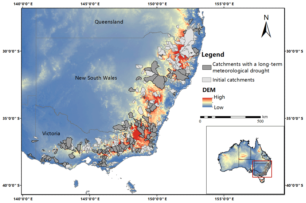
Figure 1Location map of the study catchments in southeastern Australia. The dark-gray color denotes the catchments with a long-term meteorological drought (145 catchments), while the light-gray color denotes the catchments without any sustained droughts or that have more than one prolonged drought period (253 catchments). DEM: digital elevation model.
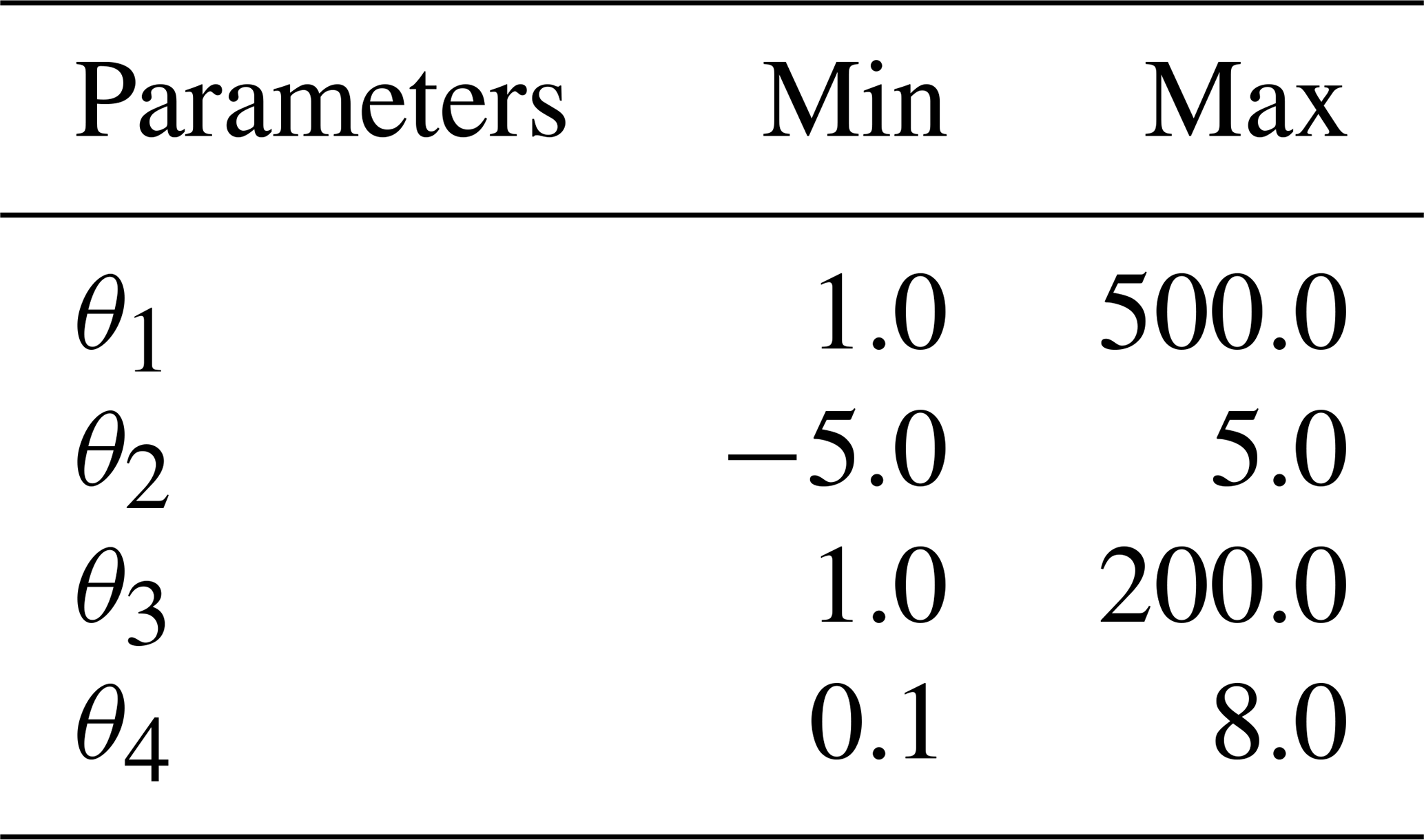
Table 1Prior ranges of parameters in the GR4J hydrological model.
The study catchments exhibit a broad variety of climatic conditions, soils, land use, and vegetation and hydrological regimes. Generally, the study catchments have much more rainfall during the spring and winter seasons than the summer and autumn seasons. In most of the study catchments, there is no snowmelt; even if the snowmelt appears in an individual catchment, it does not have much effect on the local hydrological system because the mean elevation of these catchments is around 584 m a.m.s.l. It should be mentioned that the mean elevation of these catchments is much lower than the seasonal snow line (1500 m a.m.s.l.) in this area (Saft et al., 2015).
Table 2Potential factors for exploring the association between the change of the CWSC with catchment properties and climate characteristics.

AWHC: available soil water holding capacity; Ks: saturated hydraulic conductivity; Cv: coefficient of variation.
2.2 Research data
The following data have been used in this study: (1) climate variables, including daily rainfall and daily potential evapotranspiration; (2) daily streamflow observation at the catchment outlet; (3) land use types at 1 km resolution; (4) soil types at 30 arcsec resolution; and (5) catchment attributes, including catchment area, mean elevation and so on. The detailed lists of the catchment attributes and climate characteristics are presented in Table 2. The climate variables, daily runoff and catchment attribute data were obtained from the Australian Water Resources Assessment (AWRA) system, which has served as a standard publicly available national dataset for hydrological-model evaluation (https://publications.csiro.au/rpr/pub?pid=csiro:EP113194, last access: 27 August 2020; Zhang et al., 2013). For all catchments, there are no missing data in the rainfall and potential evapotranspiration data, while the runoff data in some catchments are missing. The dataset of soil types was obtained from the Harmonized World Soil Database by the Food and Agriculture Organization of the United Nations (http://www.fao.org/soils-portal/soil-survey/soil-maps-and-databases/harmonized-world-soil-database-v12/en/, last access: 27 August 2020; Fischer et al., 2008) and was classified according to the soil texture triangle of the USDA (https://www.nrcs.usda.gov/wps/portal/nrcs/detail/soils/survey/?cid=nrcs142p2_054167, last access: 27 August 2020). The dataset of the land use types was derived from the global land cover map released by the University of Maryland (UMD) (Hansen et al., 2000) and was classified according to the UMD Land Cover Classification method (http://app.earth-observer.org/data/basemaps/images/global/LandCover_512/LandCoverUMD_512/LandCoverUMD_512.html, last access: 27 August 2020).
In total 398 catchments from southeastern Australia were selected from the original dataset, under the conditions that (1) they are not regulated and only had insignificant effects of human activities during the observation period and that (2) the catchment area ranges from 50 to 17 000 km2. Available records of these catchments for our study ranged from 1 January 1976 to 31 December 2011. For the initial dataset of 398 catchments from southeastern Australia, a set of 125 catchments were excluded before analysis because the completeness of daily streamflow data in these catchments is less than 80 %. The remaining 273 catchments are used for the identification of meteorological droughts. Finally, 145 catchments within the subset were identified with a long-term meteorological drought (see Sects. 3.1 and 4.1) and analyzed further. The attributes of the 145 catchments are summarized in Table S1 in the Supplement.
This section presents the methodology of this study, including (i) the identification of catchments with a long-term meteorological drought (Sect. 3.1); (ii) derivation of change in the CWSC on account of drought based on the hydrological-modeling method (Sect. 3.2), including an introduction of the hydrological model adopted, the likelihood function, the model parameter estimation method and the identification method for the change points of the CWSC; and (iii) potential variables that might be associated with the changes in the CWSC (Sect. 3.3).
3.1 Identification of meteorological drought
Since rainfall is one of the most important factors that influence the degree of wetness, the identification method of meteorological drought was only based on the annual rainfall data as in other studies (Li et al., 2020; Pan et al., 2019b; Saft et al., 2015; Wong et al., 2013). The method proposed by Saft et al. (2015) was introduced in this study to define the meteorological-drought period (also known as dry period). Saft et al. (2015) examined several algorithms for the identification of the dry period with the consideration of different combinations of the dry-period anomaly (i.e., the percentage variation between the annual rainfall during the dry period and the average of the whole time series), the length of the dry period and various boundary conditions, and the delineation results of the dry period by one of the algorithms that illustrated the lowest dependency on the algorithm itself and was robust to different algorithms. The process of this best identification method is generalized as follows.
Firstly, the anomaly was calculated as the percentage variation between the annual rainfall data and the long-term annual mean value, and the anomaly was smoothed with a 3-year moving window. It should be mentioned that smoothing was applied to avoid single wetter years that interrupt a long dry period and identify all periods of consecutive smoothed negative anomalies. Secondly, the start year of the dry period was defined as the start of the first 3 continuous years of the negative anomaly period based on the unsmoothed anomaly data. Similarly, the end year of the dry period was determined from the last negative 3-year anomaly series based on the unsmoothed anomaly data. The end year was defined as the last year of this 3 year series unless (i) there was a year with a positive anomaly that was larger than 15 % of the mean, in which case the end of dry period was determined as the year before that year, or (ii) the last 2 years had slightly positive anomalies (but each was smaller than 15 % of the mean), in which case the end year was determined as the first year of the positive anomaly. Two additional rules were set to ensure a sufficiently long and severe dry period: the length of the dry period should be longer than 6 years, and the mean dry years' anomaly should be smaller than 5 %. In addition, the remaining part in the observation history (except the dry period) was determined as the nondry period.
The selected algorithm has been verified as a rigorous method for processing the autocorrelation in regression residuals and testing the global significance. Furthermore, we have the same study region, i.e., catchments in southeastern Australia (but our data sources and periods are different). A more detailed process of the identification method of the dry period can be obtained in research by Saft et al. (2015) and our previous study (Pan et al., 2019b).
3.2 Derivation of the catchment response to drought
3.2.1 Hydrological model
The conceptual rainfall–runoff model, i.e., the GR4J (modèle du Génie Rural à 4 paramètres Journalier) hydrological model, was used to examine the proposed method (Perrin et al., 2003). Previous studies showed that the GR4J model had comparable simulation and prediction performance with other hydrological models with more model parameters (Pan et al., 2019a, b; Westra et al., 2014). The GR4J model comprised four parameters: θ1 represents the catchment water storage capacity (mm); θ2 denotes the coefficient of groundwater exchange (mm); θ3 represents the 1 d ahead maximum capacity of the routing store (mm); and θ4 denotes the time base of the unit hydrograph (d). Previous studies (Demirel et al., 2013; Pan et al., 2019a, b; Perrin et al., 2003; Westra et al., 2014; Yan et al., 2015) showed that θ1, which denotes the catchment water storage capacity, is the most sensitive parameter in the structure of the GR4J model.
In the GR4J model structure, the first operation is to subtract evapotranspiration from the original rainfall to determine the net rainfall or net evapotranspiration. The net rainfall is then divided into a surface flow and a water production storage of catchment, where θ1 is the maximum capacity of the production store of the catchment. The total runoff includes two flow components (underground flow and the surface runoff), which are presented as slow- and fast-routing processes by two unit hydrographs. Of the total runoff, 90 % is routed by the slow unit hydrograph and then a nonlinear routing store, while the remaining 10 % of the runoff is propagated through the fast-routing process. Both unit hydrographs depend on the same parameter θ4 expressed in days. In addition, a groundwater exchange term that acts on both flow components is calculated based on parameters θ2 and θ3. More details about the Gr4J model can be found in Perrin et al. (2003).
The real CWSC values are hard to derive based on available data and attributes of catchments. However, the hydrological model provides a new perspective for reflecting the potential variations of the CWSC, that is, the utilization of specific model parameter(s) that represent(s) the CWSC, such as parameter θ1 in the GR4J model. Figure 2 presents an example to illustrate the impacts of the shift in the value of θ1 on the model simulation results.

Figure 2Example of the impacts on model simulation due to the different shifts in model parameter θ1 (that denotes the catchment water storage capacity). Qsim refers to the simulated streamflow.
Thus, in this study, we use the magnitude of the shift in estimated θ1 between periods before and after the change point to represent the change in the CWSC. In addition, we assume that the other model parameters θ2, θ3 and θ4 are kept constant during the periods before and after the change point, and the shift of the CWSC happens on the potential change point. The constant assumption of parameters θ2, θ3 and θ4 is a common assumption, which has been made in many previous studies, such as Westra et al. (2014) and Pan et al. (2019a, b).
3.2.2 Likelihood function, parameter estimation and inference
-
Likelihood function
For catchment c, the likelihood function in this study was adopted from Thiemann et al. (2001), which is written as
where
where p refers to the likelihood probability. , and Γ(.) indicates the gamma function. T refers to the number of time step t; c is the index of catchments; q denotes observations of streamflow; ξ represents the climate inputs of the hydrological model, including precipitation (P) and potential evapotranspiration (PET); et signifies the residual error at time step t; and τ refers to the residual-error model type (Pan et al., 2019a; Thiemann et al., 2001). When the model type of residual error is verified, parameters ω and c are unchanged values. The Gaussian distribution was used to denote the residual-error model in this study; thus τ=0 was verified. Therefore, ω(τ=0) and c(τ=0) are confirmed as and , respectively. Additionally, for all unknown quantities, uniform distributions are used as their prior distributions.
-
Inference
The estimation of the posterior distributions of all unknown quantities is based on the Shuffled Complex Evolution Metropolis (SCEM-UA) sampling method (Vrugt et al., 2003). The Gelman–Rubin convergence value (Gelman et al., 2013) was used as the evaluation criterion of model convergence, with its value that should be smaller than the threshold of 1.2. The prior ranges of all model parameters have been given in Table 1.
3.2.3 Bayesian change point analysis
In this part, the Bayesian change point analysis was introduced to find out the possible change points of the CWSC. The change point of the CWSC denotes the time point that the estimated values of the CWSC between two periods (before and after this point) were significantly different. Each change point was then illustrated by a likelihood probability. The time point with the maximum likelihood probability among all potential options was regarded as the final change point of the catchment.
The Bayesian change point is one of the simplest and most effective methods to analyze the change point problem (Cahill et al., 2015; Carlin et al., 1992). The detailed process is as follows.
At first, assume unknown value k as the potential change point of the CWSC and its value is taken from . Thus, k=T is interpreted as “no change”. Assuming the rainfall–runoff relationship, Y before the change point k is
Therefore, for all possible k, corresponding values of calibrating parameters θ(c) can be obtained through the derivation of the likelihood function with the SCEM-UA algorithm. Obviously, there were four unknown quantities (i.e., four model parameters) that need to be solved during this process.
Similarly, the rainfall–runoff relationship after the change point k is assumed as
where . Parameters θ2, θ3 and θ4 are predefined and taken from the calibrating results of the previous process. Thus, only would be calibrated in this process. The association between pc and pc′ is that the posterior distributions of θ2, θ3 and θ4 are the same.
Therefore, for every k, the likelihood function L(Y; k) becomes
The Bayesian perspective is added by placing a prior density ς(k) on Θ whence the posterior density of p(k|Y) is
Therefore, the final change point is recognized as the point that has the largest p(k | Y). It should be noted that every catchment would get a “potential change point” during the calculation process. However, these potential change points would be evaluated to judge whether there is a significant shift in the estimated θ1(θ1′) between these two periods, i.e., before k and after k. In order to speed up the calculation process, the time interval between two adjacent change point is set as 30 d.
3.2.4 Criteria in identifying catchments with a significant change in θ1
In order to derive the catchments with significant changes in the CWSC, four evaluation criteria have been used in this study.
-
The minimum NSE requirement: the values of the Nash–Sutcliffe efficiency coefficient (NSE) in two periods should be larger than 0.6. The reason for setting this requirement was to ensure the simulation results by the adopted model (the GR4J model) were reasonable for the simulation of the hydrological cycle in a catchment; thus, the estimated model parameter can truly reflect the CWSC of this catchment.
-
The minimum requirement of significant change: the difference in simulated values of the parameter θ1 between the two periods should be more than ±20 %. In other words, only the catchments with more than ±20 % changes in θ1 would be recognized as significantly changed. After comparison of several other threshold levels (such as ±5 % and ±10 %), we found that the value of ±20 % can maximally exclude the negative impacts by the heterogeneity of the available parameter sets.
-
The requirement for maximum performance degradation: the degradation of NSE values between the two periods should be no more than 20 %.
-
The requirement for the robustness of results: the initial conditions (i.e., the initial value of all unknown quantities which might have impacts on the final results) for the calculation would change three times; only the catchments that were identified as significantly changed in each time would be identified as the final changing items.
3.3 Response time of a catchment
In those catchments with a significant change in the CWSC, a time lag would usually exist between the onset of meteorological drought and the change point because of the catchment resilience. For example, Van Lanen et al. (2013) and Huang et al. (2017) indicated that the groundwater that maintained the runoff during a brief drought period thus acted as a cushion to the spread of meteorological drought to hydrological drought. However, the interactions between the surface water and groundwater would be gradually reduced because of the falling groundwater levels if the drought conditions persist for several years and even decades. The shift between the connected situation and disconnected condition usually takes some time and occurs as a delayed step change, which is also known as the time lag of the catchment. Furthermore, the vegetation and catchment soil moisture may also have an impact on the response of catchments to meteorological drought.
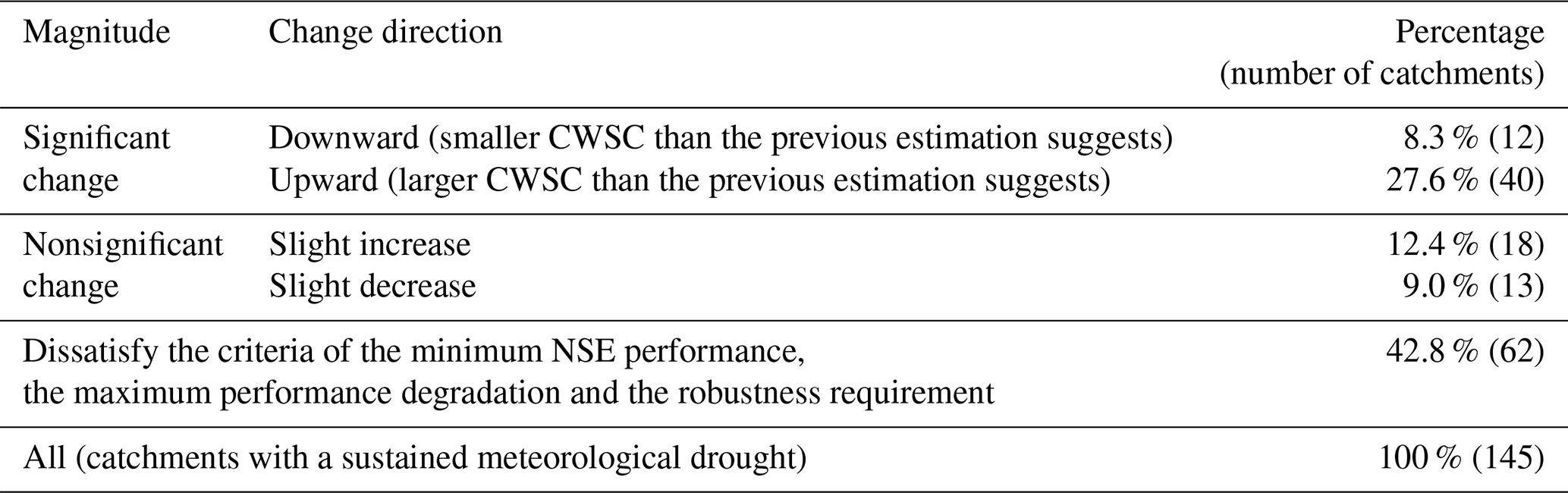
Table 3The direction of the shifts in the CWSC due to the long-term meteorological drought for the catchments in southeastern Australia. NSE: Nash–Sutcliffe efficiency.
3.4 Potential factors for the shift in the CWSC
Since the processes potentially responsible for the shift in the CWSC are not directly measured, some measurable proxies are used to explore the potential factors and possible associations between these potential factors with the changes in the CWSC and the length of the time lag of the catchment. Thus, 33 variables, including catchment physical properties and climate characteristics, were employed. It should be noted that due to the limitation of available catchment attribute data, for each catchment, only one static or constant value of the catchment property was employed (X1–X9). However, each climate variable includes four values, i.e., the values of climate characteristics during the periods before and after the change point and the variation and percent variation of the climate characteristics between the aforementioned two values. For example, four values of the average of daily runoff are considered, i.e., the average values of daily rainfall during the period before the change point ARbefore, the average values of daily rainfall during the period after the change point ARafter, and the variation and percent variation of the average of the daily runoff between ARbefore and ARafter. Table 2 summarizes the potential factors included in the following analysis. The employed climate variables can be divided into four categories, i.e., daily- (Y1–Y4), monthly- (Y5–Y7), seasonal- (Y8–Y16) and annual-scale variables (Y17–Y24). Note that the base flows of catchments were calculated based on the Lyne–Hollick method (Lyne and Hollick, 1979).
4.1 Catchments with a long-term meteorological drought
A total of 125 catchments in southeastern Australia were excluded from the original dataset (total of 398 catchments) because these catchments lacked a long enough data series during their streamflow measurement history; that is, the completeness of daily streamflow data is less than 80 %. Furthermore, 145 catchments from the filtered 273 catchments have been identified with one long-term meteorological drought during its observation history according to the identification method mentioned in Sect. 3.1. It should be mentioned that the catchments with more than one long-term drought period in its measurement history were not included in order to exclude the unnecessary impact on the subsequent evaluation of shift in the CWSC due to sustained drought. For most catchments, the long-term meteorological drought started around 2000 and then ended around 2009. The drought length of all these catchments was longer than 7 years. During this period, a decrease larger than 5 % has been identified in the annual rainfall of all those catchments.
4.2 Catchments with significant and nonsignificant change
The Bayesian change point test was applied to the 145 catchments that have been identified with a long-term meteorological drought (Table S1). Based on the evaluation criteria mentioned in Sect. 3.2.5, it was found that 83 of the 145 catchments satisfied the requirements for minimum NSE performance and maximum performance degradation. The following analysis was based on these 83 catchments.
As presented in Table 3, in 52 out of 83 (62.7 %) catchments, the estimated value of the model parameter θ1 was detected to have a significant change after the onset of meteorological drought, indicating the potential changes of the CWSC in these catchments. These catchments satisfied all criteria mentioned in Sect. 3.2.5. More clearly, the median estimated value of parameter θ1 during the period after the change point was significantly different from that value before the change point; the median NSE performance of both parameter sets in two periods were larger than 0.6; furthermore, the performance degradation between simulated results before and after the change point was no more than 20 %. Meanwhile, the remaining 31 (37.3 %) catchments had no significant changes after the onset of the drought.
Figure 3 illustrates the results of three examples, including the posterior distributions of θ1 during the periods before and after the change point (left three columns), the posterior probability in the likely change points (middle three columns) and the corresponding NSE performance (right three columns). Clearly, there was a time lag between the onset of meteorological drought and the shift in the CWSC. In catchment 215002, a significant upward change in θ1 was detected after the change point. It means that after the change point the CWSC was larger than expected based on the calibrated results in two periods. As for the posterior probability, it was found that there was a probability of 48.0 % that the change point would be located in the range of July–December in 2001 and a probability of 76.0 % that the change point would be located in the range of February–December in 2001. In catchment 401203, the white box that refers to the mean estimate of θ1 was shifted downward significantly, indicating the potential decreased change in the CWSC of this catchment. The likely change point has a probability of 39.9 % to occur within the period of January–July in 2003. Finally, catchment 410061 experienced an upward but not significant change in θ1 when comparing the results from two periods that were separated by the “most likely change point”. Since the shift in θ1 was not significant in this catchment, the change point did not exist here statistically. Thus, under sustained rainfall reduction, the CWSC of different catchments might experience absolute diverse changes. The possible reasons may lie in the diverse catchment properties and climate characteristics (see Sect. 4.4 and 4.5).
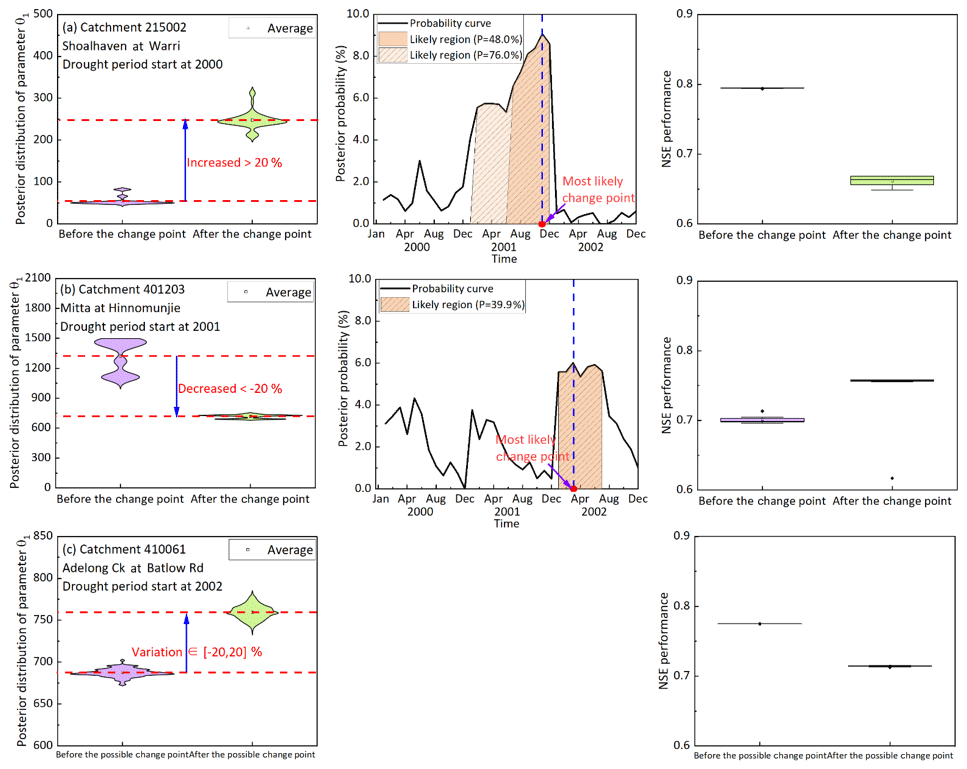
Figure 3Examples of shifts in model parameter θ1: (a) catchment 215002 with a significant upward change in θ1, (b) catchment 401203 with a significant downward change in θ1 and (c) catchment 410061 with a nonsignificant change in θ1. The first column compares the posterior distributions of θ1 calibrated during the periods before and after the change point. The second column denotes the posterior probabilities based on all possible change points. The last column denotes the Nash–Sutcliffe efficiency (NSE) performance of the model parameters calibrated during the periods before and after the most likely change point.
4.3 Direction and magnitude of the shift in the CWSC
In the case of the direction of shift in the CWSC, a significant increase in the estimated θ1 has been found in 40 out of 83 catchments. Since the significant decrease in rainfall has been found during the prolonged drought, these catchments were expected to experience a downward trend with a similar magnitude of reduction in the runoff generation. However, the increase of the CWSC means that the drought might result in lower runoff generation rates for similar amounts of rainfall during the drought period. Thus, in the following years with reduced rainfall, lower runoff due to the reduced rainfall could be expected; furthermore, the even less runoff than historical records may occur because of the significant increase in the CWSC. Another 12 catchments had a significant downward shift in the CWSC. The decrease of the CWSC indicates that meteorological drought might result in higher runoff generation rates for a similar amount of rainfall than previous records. These catchments had the lower capacity to hold available water, and their ecosystems might suffer more frequent and more severe extreme events, e.g., droughts and floods. In addition, the remaining 31 catchments were divided into two parts further, i.e., 18 catchments with a slight (nonsignificant) increase in the CWSC and 13 catchments with a slight (nonsignificant) decrease in the CWSC. As for the geographical distribution of the catchments with significant and nonsignificant changes in the CWSC, Fig. 4 illustrates that there is some tendency for clustering, e.g., (1) for the majority, adjacent catchments tend to have same change directions; (2) catchments in southwestern and southern Victoria experienced different levels of increase in the CWSC, while (3) in northeastern Victoria, the majority of catchments had a decrease in the CWSC. Figure 5 presents the statistical histograms of catchments with different degrees of the shift in θ1. It should be noted that both catchments with significant changes and nonsignificant changes have been plotted together. The fitted curves in Fig. 5a and b are both positively biased, since there was a larger number of catchments with an increasing trend in the CWSC compared to those with a decreased trend detected. The distribution of the catchments illustrates that the majority of catchments have [−50, 100] percent change (based on the period before the change point) or [−100, 200] absolute change in the estimated value of θ1.
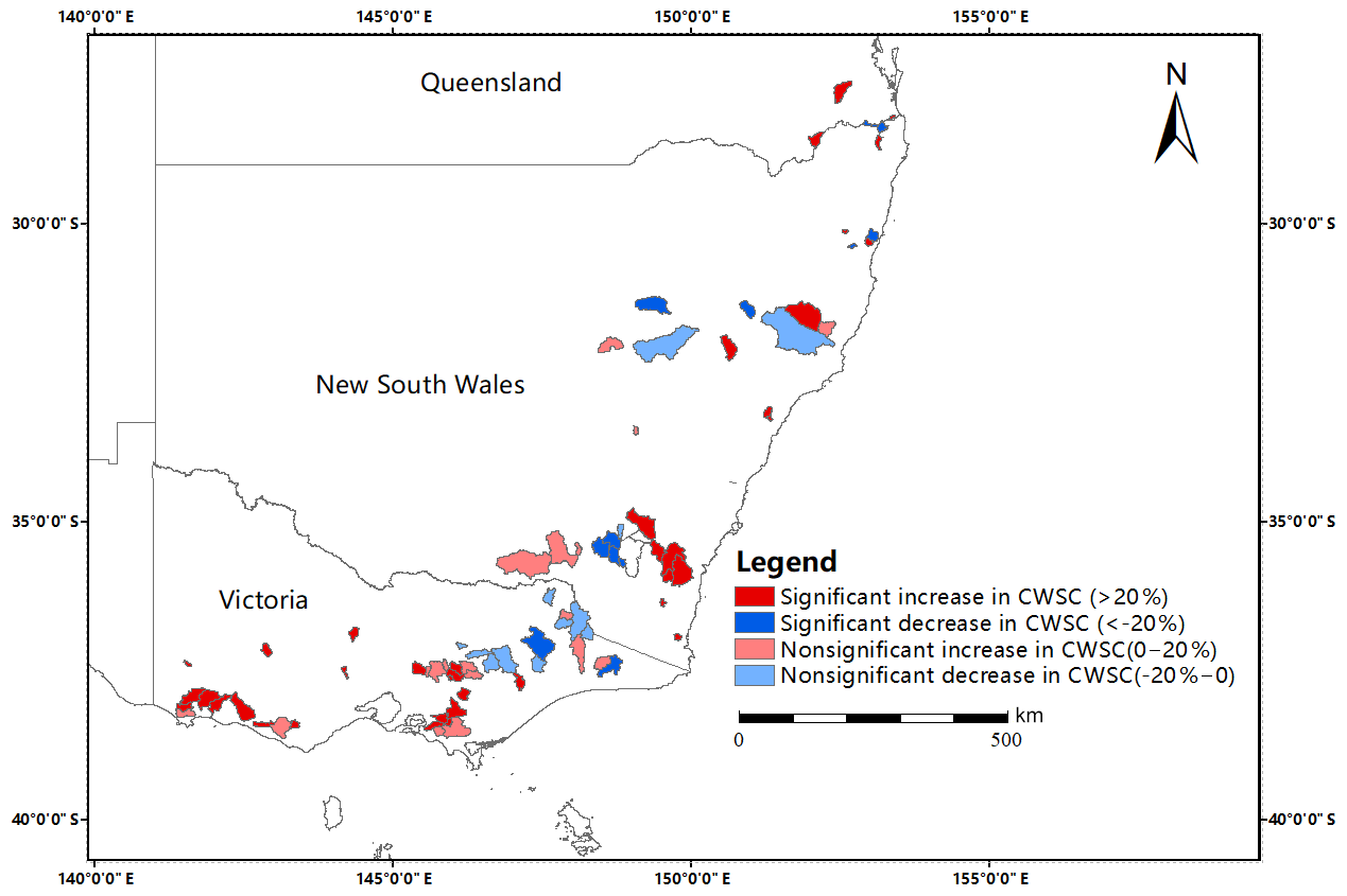
Figure 4Location map of the catchments with significant and nonsignificant shifts in the CWSC. The red (blue) color denotes the catchments that have a significant increase (decrease) in the CWSC after the change point, while the (light-blue) light-red color denotes the catchments with a nonsignificant increase (decrease) in the CWSC.
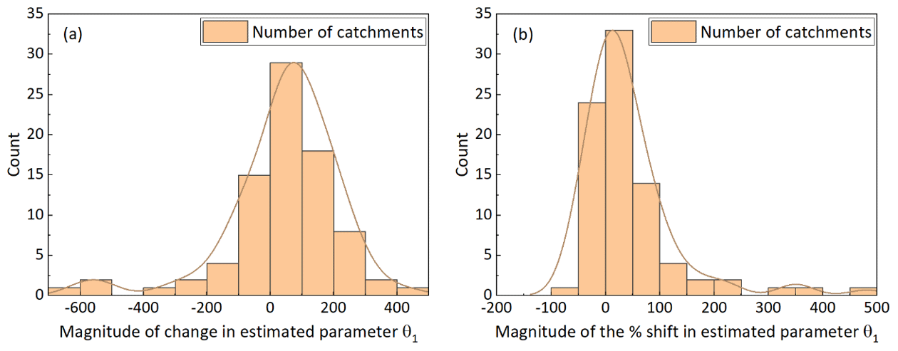
Figure 5Shift magnitudes of the CWSC between the periods before and after the change point. The orange lines denote the kernel smoother curve of the histograms.
4.4 Factors for shifts in the CWSC
In this part, we investigate whether changes in the CWSC are associated with particular catchment properties or climate characteristics. In other words, do catchments with certain catchment properties or climate characteristics more easily trigger the potential shift in their CWSC?
4.4.1 Factors for the significant and nonsignificant shifts in the CWSC
Two groups of catchments were established according to the significance level of the shift in θ1 after the onset of the long-term drought. Specifically, one group is composed of catchments with a significant change in the estimation of parameter θ1 between two periods. The other group is composed of catchments that only had a nonsignificant change in parameter θ1 between two periods. As shown in Fig. 6 (left two columns), the catchment properties of two groups of catchments have been presented. Significant changes in the CWSC were likely to occur in catchments with smaller catchment areas, lower elevation and difference, less slope, lower available soil water holding capacity (AWHC) in subsoil, and less saturated hydraulic conductivity (Ks) in topsoil. The forest coverage percentage and the AWHC in topsoil are not significantly different between the two groups of catchments. It should be noted that some of those catchment properties might be somewhat related. Thus, the Pearson correlation coefficient (PCC) has been used to explore the potential relationship between the change in parameter θ1 with the catchment properties as well as the connection between different catchment properties. Figure 7 illustrates a low degree of association between the percentage shift in parameter θ1 and these catchment properties for two groups of catchments.
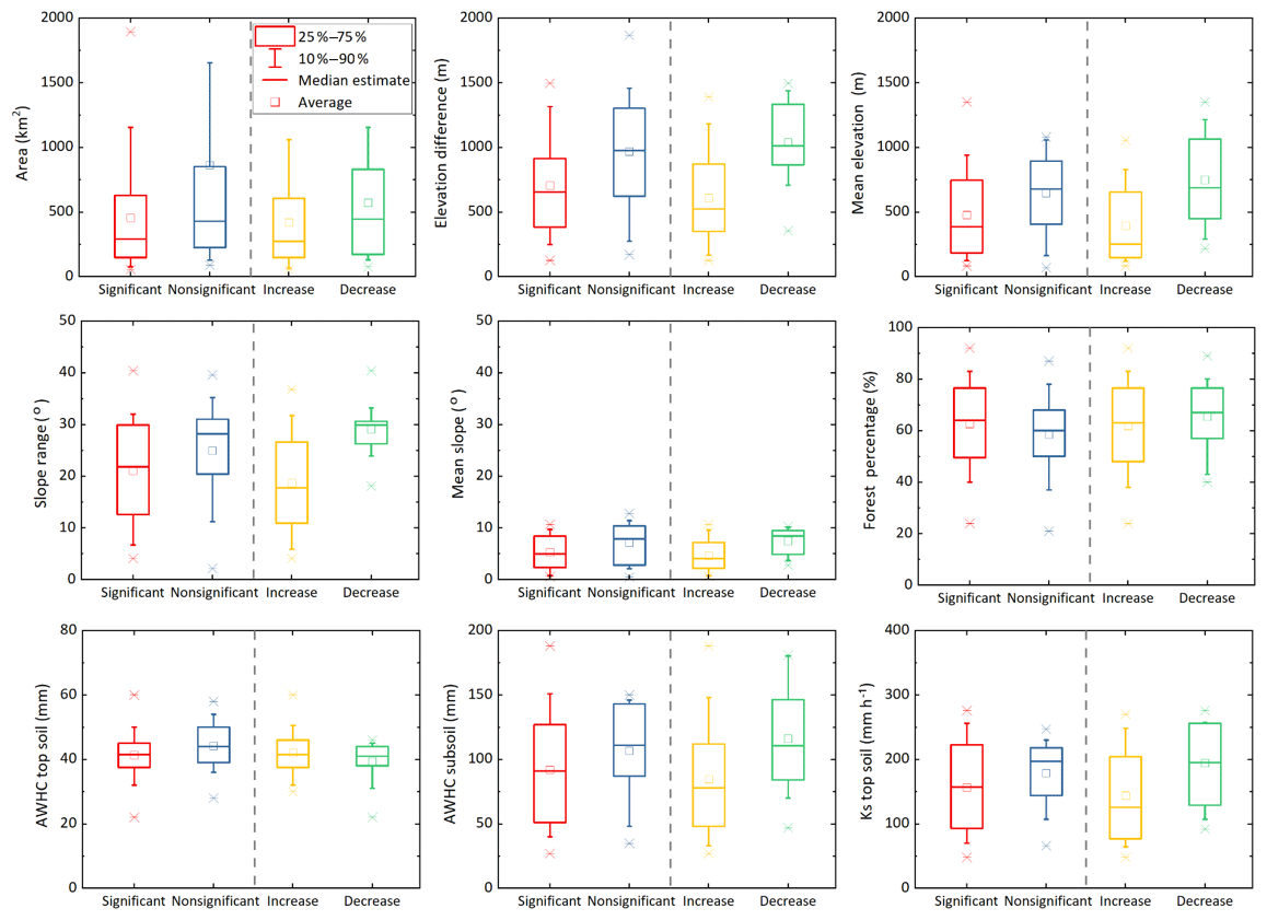
Figure 6Catchment properties for the study catchments, including catchment area (km2), elevation difference between the maximum and minimum elevations (m), mean elevation (m), slope range (∘), mean slope (∘), forest coverage percentage (%), available soil water holding capacity (AWHC) in top- and subsoils, and saturated hydraulic conductivity (Ks) in topsoil (mm h−1). The red and black lines (solid) denote the average of catchments with and without significant changes in the CWSC, respectively. “Increased” means catchments with a significant increase in the CWSC, while “decreased” represents catchments with a significant decrease in the CWSC.
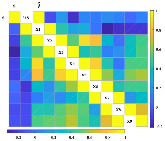
Figure 7Pearson correlation coefficient based on the association between the magnitude of the shift in θ1 and multiple catchment properties as well as the associations between different catchment properties. In the lower triangular matrix, the shift in θ1 was considered, while in the upper triangular matrix, the percentage shift in θ1 was used. S denotes the shift in θ1, and %S denotes the percentage shift in θ1, while X1–X9 denotes the catchment properties mentioned in Table 2.
4.4.2 Factors for the significant upward and downward shifts in the CWSC
Two subgroups of catchments were extracted from the group of catchments with significant shifts in the CWSC according to the change direction of the estimated θ1. Specifically, one subset is composed of catchments with a significant upward change in the estimated θ1, while another subset is composed of catchments that experienced a significant downward shift in the estimated θ1. As shown in Fig. 6 (right two columns), catchments with a significant upward change in estimated θ1 had a smaller catchment area, lower elevation and difference, less slope, lower AWHC in subsoil, and less saturated hydraulic conductivity (Ks) in topsoil. The forest coverage percentage, the AWHC in topsoil and the length of the time lag are not significantly different between two subgroups of catchments.
Furthermore, 24 climate variables in Table 2 have been used to explore the difference between two subgroups of catchments and the possible associations between the magnitude of the shift in the CWSC with the values of climate variables. As illustrated in Sect. 3.4, one climate variable consists of four values, i.e., the climate values during the periods before and after the change point, absolute difference, and percentage variation between the climate variables between two periods. Thus, there were 96 climate values considered in this part. As shown in Fig. 8, significant differences (i.e., percentage variation is larger than ±10 %) have been found in the majority of the climate variables between two subgroups of catchments for both four categories of climate values, except for the percentage difference in the daily maximum temperature, which was not significant for both four values between two periods. In addition, the percentage difference of the drought length (≥7 years) between the two subgroups of catchments was 14.3 %, and on average, the subset of catchments with significantly increased shift had longer drought length than the other subset.
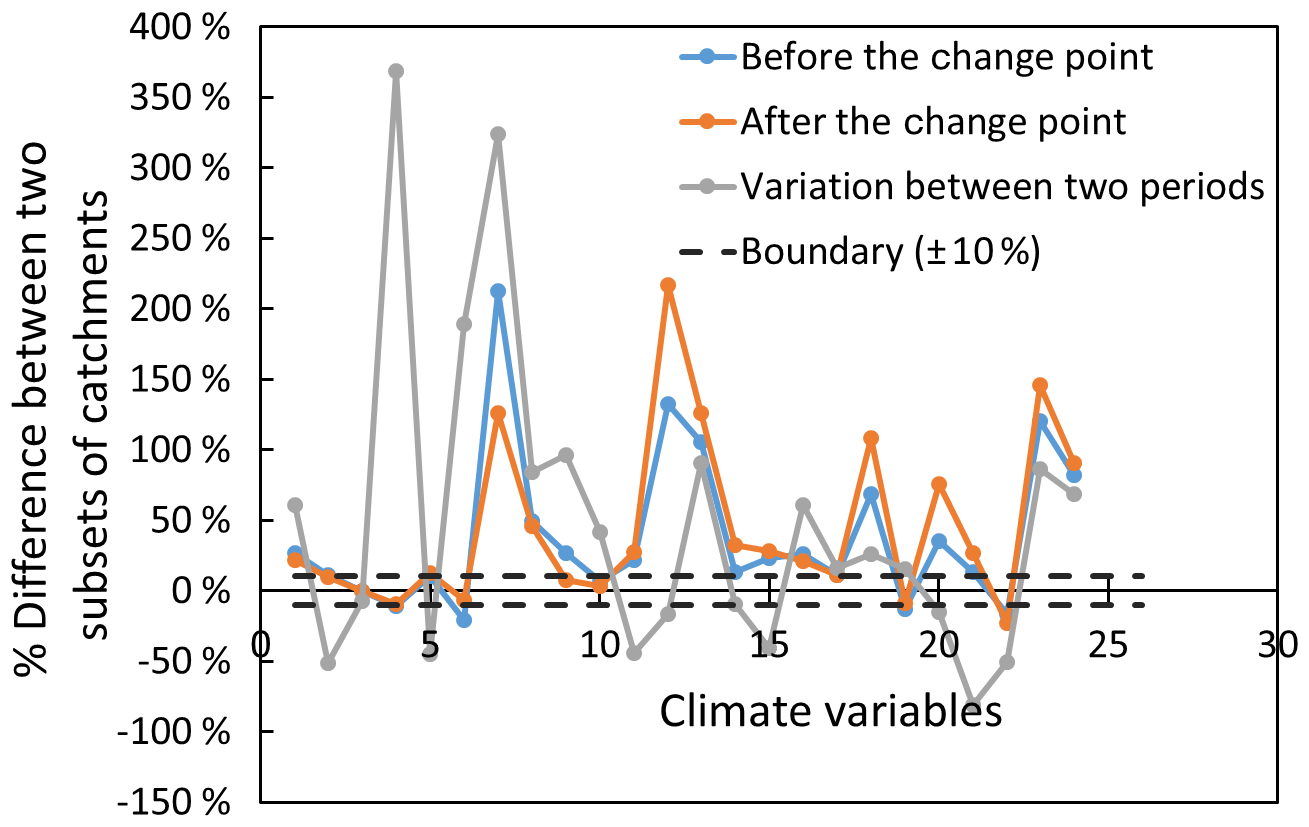
Figure 8The percentage difference of climate variables between two subgroups of catchments (catchments with significant upward and downward changes in estimated θ1). The numbers in the x coordinate denote climate variables illustrated in Table 2. The blue and orange lines denote the percentage difference of climate variables between two subgroups of catchments during the periods before and after the change point, respectively. The gray line denotes the percentage difference of the amplitude of variation between two periods. The positive value means an increase, while a negative value means a decrease.
The potential associations between the change in the CWSC and both climate values have been presented in Fig. 9. A medium degree of correlation (PCC >0.4) has been found between the percentage shift in the CWSC with the Cv of annual rainfall (PCC =0.422) and the Cv of annual runoff (PCC =0.419) during the period before the change point. No more than a medium degree of correlation has been found between the shift in the CWSC and the climate values after the change point. As for the variation of climate values between two periods, a larger association has been found in the shift in the CWSC with the variation in daily rainfall (PCC ), variation in annual rainfall (PCC ) and change in annual runoff ratio (PCC =0.479) rather than others. In addition, it seems that the shift in parameter θ1 was not related to drought length (≥7 years) because its PCC value was only 0.148.
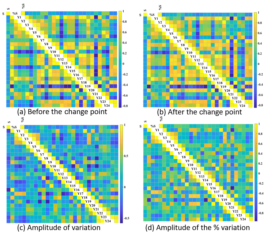
Figure 9Pearson correlation coefficient based on the association between (1) the magnitude of shifts in the CWSC with multiple climate variables as well as the connection between different climate variables (lower triangular matrix) and (2) the magnitude of percentage shifts in the CWSC with multiple climate variables as well as the connection between different climate variables (upper triangular matrix). Panels (a) and (b) denote a connection between the shift or percentage shift in the CWSC with the climate variables during the periods before and after the change point, respectively. Panels (c) and (d) denote the association between the shift or percentage shift in the CWSC with the variation and percentage variation of climate variables of two periods, respectively. Y1–Y24 denotes the climate variables in Table 2.
4.5 Factors for the time lag of a catchment
Using the same method as illustrated in Sect. 4.4, the difference between two subgroups of catchments and potential associations between the time lag of the catchment (time lag) with catchment properties and climate characteristics were analyzed. In other words, is it easier for catchments with certain catchment properties and/or climate conditions to have longer time lag? It should be noted that the catchments with a nonsignificant change in the CWSC were not included in this part, because these catchments did not experience a significant change in its estimation value of θ1 and thus did not have a statistically significant change point.
On average, the time lag in the subset of catchments with the significant upward change in estimated θ1 was 9.4 % larger than the subset with a significant downward shift. As shown in Fig. 10, only lower associations have been found between the time lag with different catchments. The maximum PCC value between the time lag with the catchment properties was just 0.159, which was achieved by the correlation between the time lag and the AWHC in topsoil. In addition, the potential association between the time lag with the climate variables also has been presented in Fig. 11. Similarly, low correlation (|PCC<0.3|) has been found between the time lag and both four categories of climate values.
The results indicate that, under certain circumstances, a long-term meteorological drought would result in a significant change in the CWSC. In this study, 52 in 83 catchments (62.7 %) have been found to have a significant shift in their CWSC. Furthermore, a subset of 40 catchments had a significant upward change in the CWSC, while another subset of 12 catchments had a significant downward change.
5.1 Possible reasons for different changes in the CWSC
The results indicate that, under certain circumstances, a long-term meteorological drought would result in a significant change in the CWSC. However, no strong association has been found between the magnitude of the change in the CWSC with any single variable. In addition, the length of the dry period was not associated with the shift in the CWSC. Thus, it seems that the catchment response behavior to long-term meteorological drought is controlled by the combination of local catchment properties and climate characteristics rather than a single factor. Thus, further studies are still required to confirm which factors played the most important role in the catchment dynamic.
5.1.1 Potential mechanisms for the impacts of catchments properties on the CWSC
The CWSC of a catchment is the comprehensive presentation of catchment properties in the field of water storage. The interrelated impacts by the changes in catchment properties, such as groundwater decline, may result in the potential shift in the CWSC. However, it should be mentioned that even similar changes that take place in catchments with different backgrounds of properties may have opposite impacts on the change direction of the CWSC.
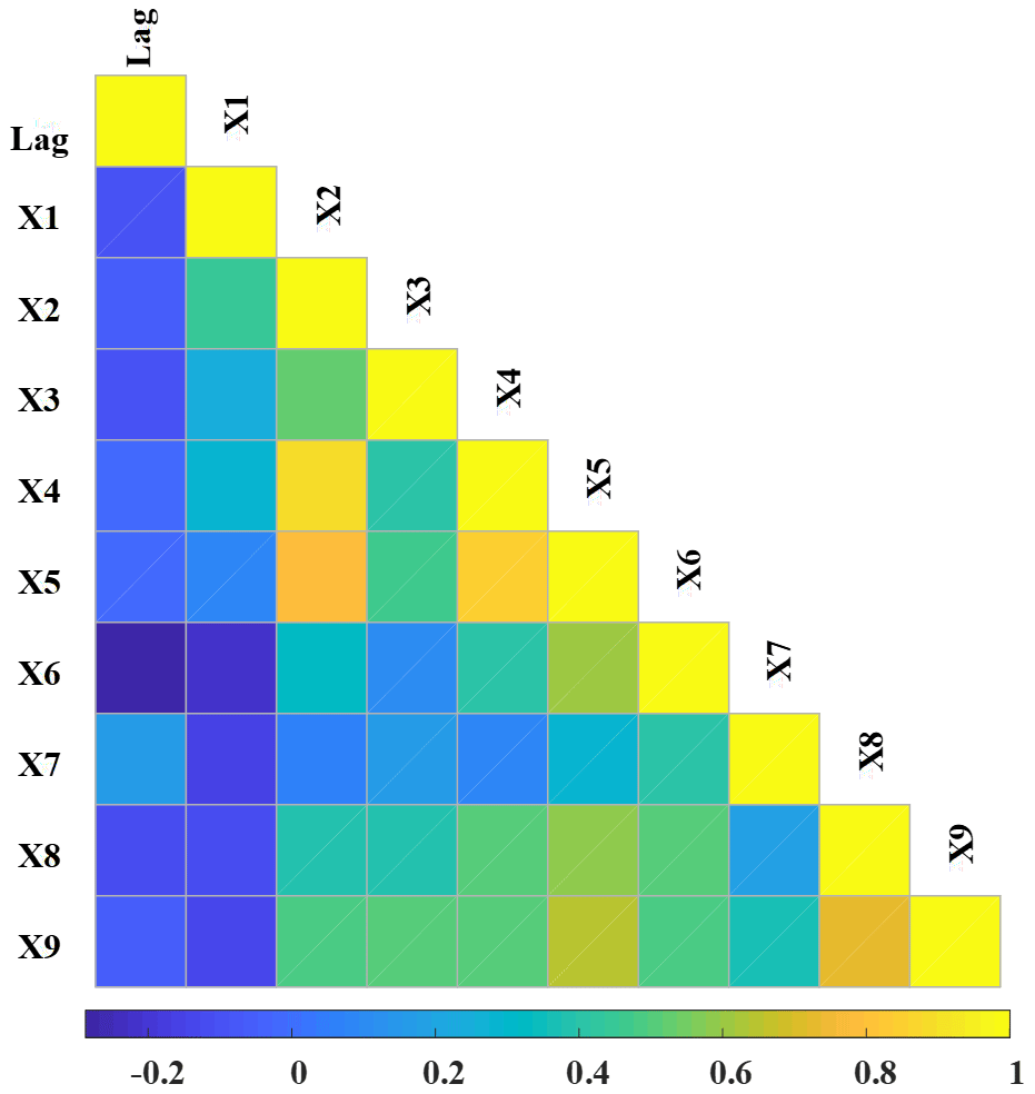
Figure 10Pearson correlation coefficient based on the length of the time lag of the catchment (between the start of the meteorological drought and the change point) with the catchment properties.
In the study area, the groundwater decline combined with a different background of soil types in the catchments may be one of the possible reasons for different change directions in the CWSC. The groundwater decline would lead to the loss of the hydraulic connection between groundwater and surface water. The space that once was occupied by soil water becomes void. However, catchments with different soils would have different change directions. In sand and other soil types with a lower adhesive property, these soil pores would be compacted due to the reduction of buoyancy of soil water; thus the compacted soil may result in a decrease in the CWSC. Conversely, these soil pores may be retained in those soils with a strong adhesive property; the decline of groundwater may lead to an increase in the CWSC. A significant decline in the groundwater level has been observed in southeastern Australia during the drought periods (Leblanc et al., 2009). Figure 12 presents the soil types of 83 catchments in southeastern Australia and illustrates that the silt loam and loam are the main soil types in the study area, the sum of which occupies more than 80 % of the region. Moreover, southwestern Victoria and southern New South Wales (i.e., catchments with an increase in the CWSC) were mainly occupied by the loam, while eastern Victoria (i.e., catchments with an increase in the CWSC) was mainly occupied by the silt loam. By contrast, the silt loam had a stronger adhesive property and larger field capacity than the loam. Thus, the distribution of these two soil types may explain a proportion of variance in the change direction of the CWSC. However, in southern Victoria, the results disagree with this finding; the possible reasons might be that other more influential factors control the catchment behaviors in this region.
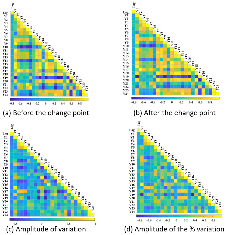
Figure 11Pearson correlation coefficient based on the association between the length of the time lag of the catchment with multiple climate variables.
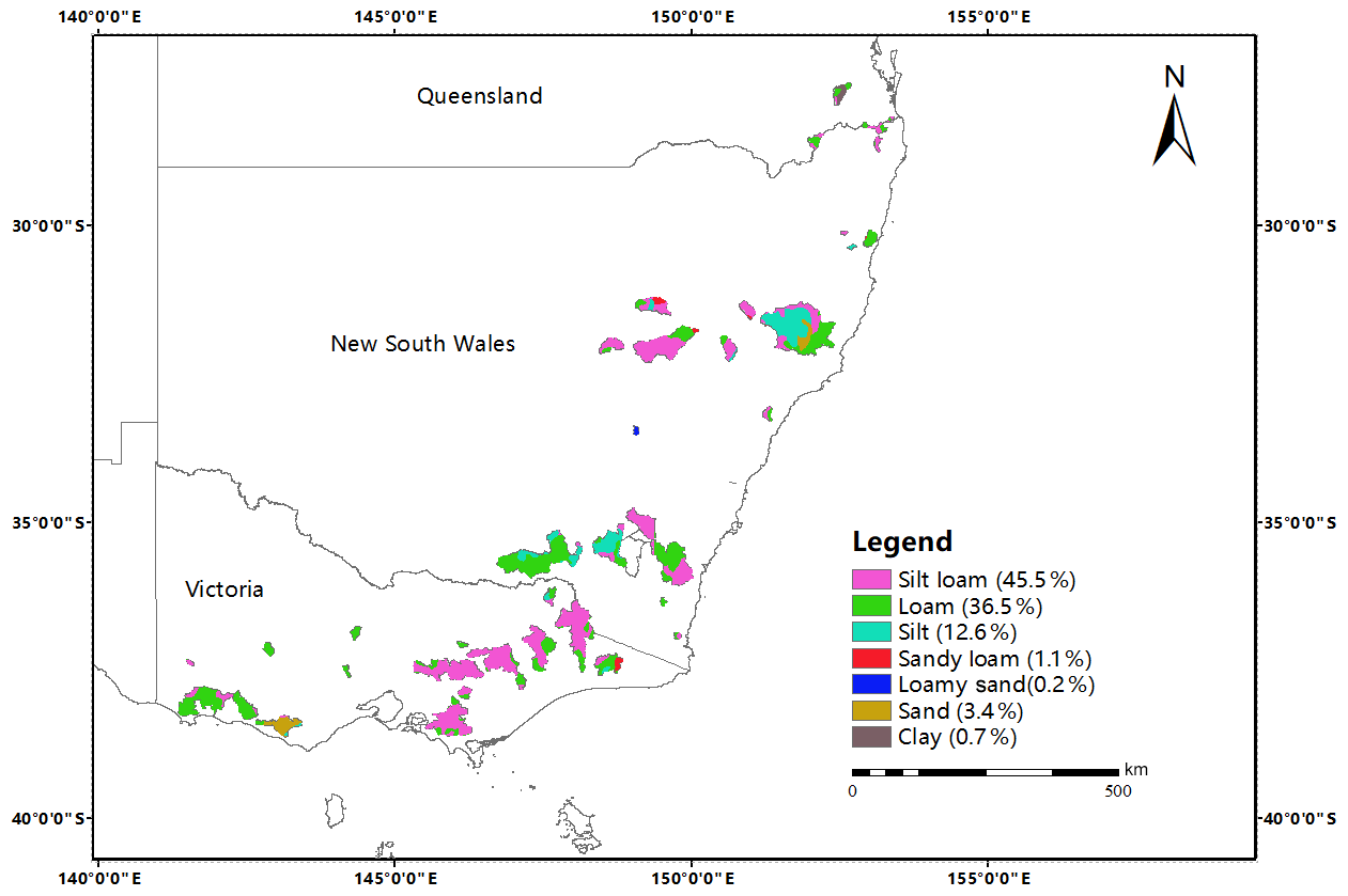
Figure 12Soil types and corresponding percentages in the study catchments (83 catchments). The soil type data was adopted from the Harmonized World Soil Database at 30 arcsec resolution (Fischer et al., 2008) and classified according to the soil texture triangle of the USDA.
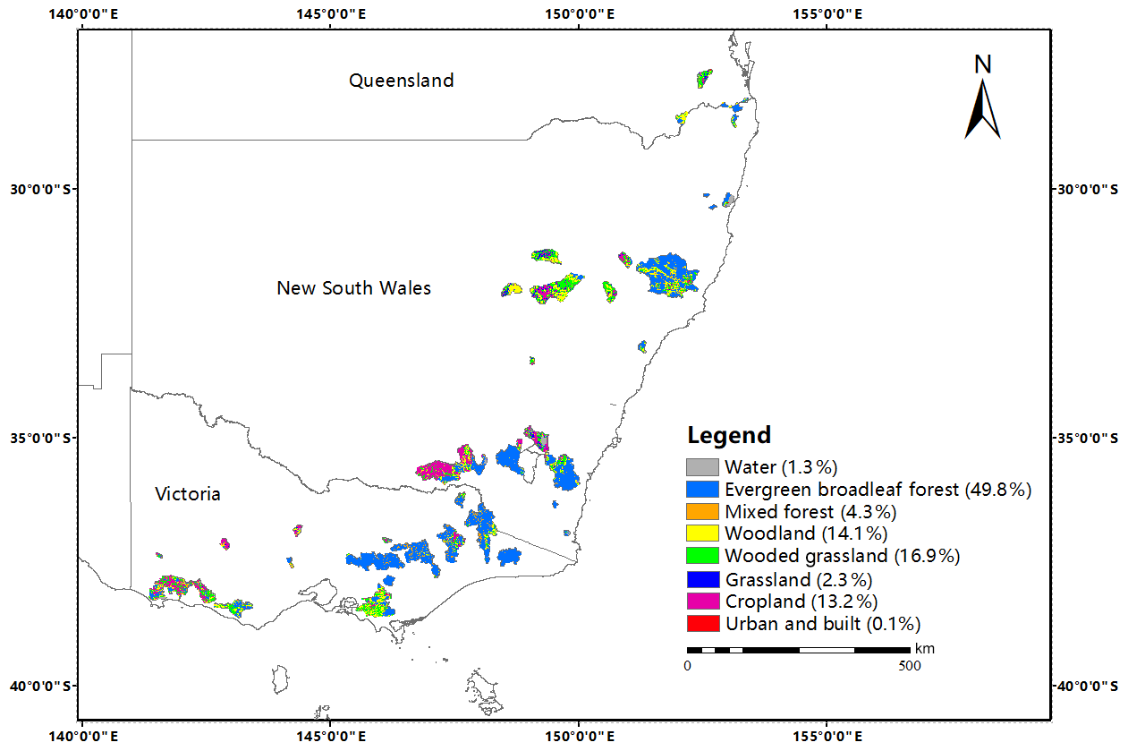
Figure 13Land use types and corresponding percentages in the study catchments (83 catchments). The land use data were adopted from the global land cover map at 1 km resolution released by the University of Maryland (Hansen et al., 2000).
In addition, another possible reason is the variance in land use. The primary land use types in the study region are evergreen broadleaf forest (49.8 %), wooded grassland (16.9 %), woodland (14.1 %) and cropland (13.2 %). As shown in Fig. 13, catchments with downward changes are mainly covered by evergreen broadleaf forest, while those with upward changes are mainly covered by other three land use types. Historical literature (Adams et al., 2012; Fensham et al., 2009; Ferraz et al., 2009) showed that, due to the persistent drought, plant mortality and change in species compositions have been observed in southeastern Australia. Thus, it can be hypothesized that evergreen broadleaf forest has less resilience in response to the drought, and it may be much easier for it to experience significant changes in the CWSC than other types, since that the growth of evergreen broadleaf forest needs much more water than other types. In catchments with large coverage of evergreen broadleaf forest, the canopy interception and absorption of the forest usually consist of the vital proportions for the catchments to store water; thus the tree die-off in these catchments might result in a decrease in the CWSC. On the contrary, in the catchment with other land use types, the water storage by its vegetation may only play a non-primary role, and its vegetation has a stronger resilience in response to the drought because of less water consumption. Thus, the persistent drought in these catchments did not result in massive tree morality but merely led to the increased water stress and the augmentation of the CWSC.
5.1.2 Potential mechanisms for the impacts of climate characteristics on the CWSC
The effect mechanism of climate characteristics on the CWSC is through their remodeling on the catchment properties. A medium degree of correlation has been found between the percentage shift in the CWSC with the coefficients of annual rainfall and runoff before the change point and the variation in annual or daily rainfall and annual runoff ratio. Furthermore, the shift in the CWSC was not associated with all climate variables after the change point. It also has been found that the annual distribution of baseflow and the interannual, seasonal and monthly distribution of rainfall and runoff are not correlated to the shift in the CWSC. Previous studies (Chiew et al., 2011; Saft et al., 2015) illustrated that during the meteorological drought, a large reduction in autumn rainfall and an even larger decrease in winter runoff and annual runoff of many catchments in southeastern Australia have been observed. However, in our study, significant declines in rainfall and runoff in all four seasons have been observed throughout the study area, not merely the autumn rainfall and winter runoff. Furthermore, significant differences have been found in most climate variables between catchments with significant upward and downward changes, including the autumn rainfall and winter and annual runoff and other climate variables. Thus, it is really hard to judge the influence of each factor on the CWSC. According to our study, it seems that the final changes in the CWSC are the combined effects of multiple climate variables and catchment properties.
5.2 Catchments with quick or slow response
The length of time lag represents the resilience of a catchment in response to a prolonged drought. Our results indicated a negative association between the length of time lag with the forest coverage percentage in both catchments with significant upward and downward changes. It means that catchments with a larger forest coverage percentage are more susceptible to the stress from a chronic meteorological drought than other catchments. This phenomenon is possibly related to the primary land use types in the study area, i.e., evergreen broadleaf forest (49.8 %), which has a high demand for water consumption. Thus, a catchment that experienced a prolonged meteorological drought, combined with the characteristic of large coverage of evergreen broadleaf forest, would be quite sensitive to have changes in its CWSC. In addition, opposite directions of PCC association between the time lag with several catchment properties (i.e., mean elevation and elevation difference, mean slope and slope range, AWHC in subsoil, and Ks in topsoil) have been found in two subgroups of catchments. For example, in the subset of catchments with a significant decrease in the CWSC, the length of time lag is positively associated with the elevation level and slope, while in the subset of catchments with a significant increase in the CWSC, it is a negative association. Similar findings also have been found in associations between the time lag and multiple climate variables (e.g., daily rainfall and baseflow). However, since only a low association level has been observed between the time lag and these single climate variables, it is still hard to judge whether there are certain physical mechanisms behind this phenomenon or it is just a statistical artifact.
This study aims to examine the possible changes in the catchment water storage capacity (CWSC) as well as the time lag between the onset of the meteorological drought and the change point of the CWSC. A classical hydrological model, GR4J, was used, and its parameter θ1 was selected to denote the CWSC. Thus, the temporal variation in parameter θ1 was detected to reveal the possible fluctuation in the CWSC, and the causality between the temporal variation in parameter θ1 and a persistent meteorological drought was examined. The 83 catchments in southeastern Australia were selected as the study areas because a decadal meteorological drought was observed. Main conclusions can be drawn as follows.
-
Significant changes in the CWSC have been identified in 62.7 % (52 in 83) of catchments, which can be divided into two subgroups with opposite catchment responses: 48.2 % (40 in 83) experienced a significant decrease in the CWSC during the drought period and had lower runoff generation rates, while 14.5 % (12 in 83) of catchments experienced a significant decrease in the CWSC during the drought period and had higher runoff generation rates.
-
Different change directions in the CWSC resulted in the opposite impacts on runoff generation, i.e., catchments with increased CWSC would result in lower runoff generation rates for similar amounts of rainfall than before, while those catchments with decreased CWSC would have an opposite response (higher runoff generation rate). Generally, the increase in the CWSC during a chronic drought can be observed in smaller catchments with lower elevation, slope and forest coverage of evergreen broadleaf forest, while the decrease in the CWSC can be observed in larger catchments with higher elevation and larger coverage of evergreen broadleaf forest. Among all catchment properties and climate variables considered, our results suggest that two climate variables (i.e., variation in annual rainfall and annual runoff ratio) have the strongest associations with the shift in the CWSC.
-
The responses of different catchments to persistent meteorological drought were not equally susceptible. Catchments with a lower proportion of evergreen broadleaf forest usually have a longer time lag and are more resilient.
It is noted that although this study resulted in interesting findings that give new insight and have not been fully outlined before, it is based on the lumped GR4J model and the specific case in Australia, which implies that the main findings and conclusions may not directly extendable to other regions. Thus, to examine the generality of the main conclusions, the response of the CWSC to meteorological drought can be analyzed with other hydrological models in other regions.
The data and code that support the findings of this study are available from the corresponding author upon reasonable request.
The supplement related to this article is available online at: https://doi.org/10.5194/hess-24-4369-2020-supplement.
ZP and PL conceived the study and wrote the paper. CYX, LC and JT made constructive comments on the writing of this study, which improved the quality of this paper. SC and KX provided the catchment attribute data and made comments. All of the authors read and approved the paper.
The authors declare that they have no conflict of interest.
This research is funded in part by the National Key Research and Development Program (grant no. 2018YFC0407202), the National Natural Science Foundation of China (grant nos. 51861125102, 51879193 and 41890822), and the Natural Science Foundation of Hubei Province (grant no. 2017CFA015). The authors appreciate the help from the Supercomputing Center of Wuhan University for providing necessary guides to perform the numerical calculations of this study on the supercomputing system.
This research has been supported by the National Key Research and Development Program (grant no. 2018YFC0407202), the National Natural Science Foundation of China (grant nos. 51861125102, 51879193 and 41890822), and the Natural Science Foundation of Hubei Province (grant no. 2017CFA015).
This paper was edited by Dominic Mazvimavi and reviewed by two anonymous referees.
Adams, H. D., Luce, C. H., Breshears, D. D., Allen, C. D., Weiler, M., Hale, V. C., Smith, A. M. S., and Huxman, T. E.: Ecohydrological consequences of drought- and infestation- triggered tree die-off: insights and hypotheses, Ecohydrology, 5, 145–159, https://doi.org/10.1002/eco.233, 2012.
Cahill, N., Rahmstorf, S., and Parnell, A. C.: Change points of global temperature, Environ. Res. Lett., 10, 084002, https://doi.org/10.1088/1748-9326/10/8/084002, 2015.
Carlin, B. P., Gelfand, A. E., and Smith, A. F. M.: Hierarchical Bayesian-Analysis of Changepoint Problems, J. R. Stat. Soc. Ser. C-Appl. Stat., 41, 389–405, 1992.
Chiew, F. H. S., Young, W. J., Cai, W., and Teng, J.: Current drought and future hydroclimate projections in southeast Australia and implications for water resources management, Stoch. Environ. Res. Risk Assess., 25, 601–612, https://doi.org/10.1007/s00477-010-0424-x, 2011.
Dai, A.: Increasing drought under global warming in observations and models, Nat. Clim. Change, 3, 52–58, https://doi.org/10.1038/nclimate1633, 2012.
Dai, A. G.: Drought under global warming: a review, Wiley Interdisciplinary Reviews-Climate Change, 2, 45–65, https://doi.org/10.1002/wcc.81, 2011.
Demirel, M. C., Booij, M. J., and Hoekstra, A. Y.: Effect of different uncertainty sources on the skill of 10 day ensemble low flow forecasts for two hydrological models, Water Resour. Res., 49, 4035–4053, https://doi.org/10.1002/wrcr.20294, 2013.
Deng, C., Liu, P., Guo, S. L., Li, Z. J., and Wang, D. B.: Identification of hydrological model parameter variation using ensemble Kalman filter, Hydrol. Earth Syst. Sci., 20, 4949–4961, https://doi.org/10.5194/hess-20-4949-2016, 2016.
Descroix, L., Mahe, G., Lebel, T., Favreau, G., Galle, S., Gautier, E., Olivry, J. C., Albergel, J., Amogu, O., Cappelaere, B., Dessouassi, R., Diedhiou, A., Le Breton, E., Mamadou, I., and Sighomnou, D.: Spatio-temporal variability of hydrological regimes around the boundaries between Sahelian and Sudanian areas of West Africa: A synthesis, J. Hydrol., 375, 90–102, https://doi.org/10.1016/j.jhydrol.2008.12.012, 2009.
Fensham, R. J., Fairfax, R. J., and Ward, D. P.: Drought-induced tree death in savanna, Glob. Change Biol., 15, 380–387, https://doi.org/10.1111/j.1365-2486.2008.01718.x, 2009.
Ferraz, S. F. D., Vettorazzi, C. A., and Theobald, D. M.: Using indicators of deforestation and land-use dynamics to support conservation strategies: A case study of central Rondonia, Brazil, For. Ecol. Manage., 257, 1586–1595, https://doi.org/10.1016/j.foreco.2009.01.013, 2009.
Fischer, G., Nachtergaele., F., Prieler., S., Velthuizen, H. T. v., Verelst., L., and D. Wiberg: Global Agro-ecological Zones Assessment for Agriculture (GAEZ 2008), edited by: IIASA, Laxenburg, Austria, FAO, Rome, Italy, 2008.
Gelman, A., Carlin, J., Stern, H., Dunson, D., Vehtari, A., and Rubin, D.: Bayesian Data Analysis, third ed., CRC Press, London, 2013.
Grayson, R. B., Western, A. W., Chiew, F. H. S., and Bloschl, G.: Preferred states in spatial soil moisture patterns: Local and nonlocal controls, Water Resour. Res., 33, 2897–2908, https://doi.org/10.1029/97wr02174, 1997.
Hansen, M., DeFries, R., Townshend, J. R. G., and Sohlberg, R.: Global land cover classification at 1 km resolution using a decision tree classifier, Int. J. Remote Sens., 21, 1331–1365, 2000.
Haslinger, K., Koffler, D., Schoner, W., and Laaha, G.: Exploring the link between meteorological drought and streamflow: Effects of climate-catchment interaction, Water Resour. Res., 50, 2468–2487, https://doi.org/10.1002/2013wr015051, 2014.
Huang, S. Z., Huang, Q., Chang, J. X., Leng, G. Y., and Xing, L.: The response of agricultural drought to meteorological drought and the influencing factors: A case study in the Wei River Basin, China, Agric. Water Manage., 159, 45–54, https://doi.org/10.1016/j.agwat.2015.05.023, 2015.
Huang, S. Z., Li, P., Huang, Q., Leng, G. Y., Hou, B. B., and Ma, L.: The propagation from meteorological to hydrological drought and its potential influence factors, J. Hydrol., 547, 184–195, https://doi.org/10.1016/j.jhydrol.2017.01.041, 2017.
Leblanc, M. J., Tregoning, P., Ramillien, G., Tweed, S. O., and Fakes, A.: Basin-scale, integrated observations of the early 21st century multiyear drought in southeast Australia, Water Resour. Res., 45, W04408, https://doi.org/10.1029/2008wr007333, 2009.
Li, Q. F., He, P. F., He, Y. C., Han, X. Y., Zeng, T. S., Lu, G. B., and Wang, H. J.: Investigation to the relation between meteorological drought and hydrological drought in the upper Shaying River Basin using wavelet analysis, Atmos. Res., 27, 138–145, https://doi.org/10.1016/j.atmosres.2019.104743, 2020.
Lopez-Moreno, J. I., Vicente-Serrano, S. M., Zabalza, J., Begueria, S., Lorenzo-Lacruz, J., Azorin-Molina, C., and Moran-Tejeda, E.: Hydrological response to climate variability at different time scales: A study in the Ebro basin, J. Hydrol., 477, 175–188, https://doi.org/10.1016/j.jhydrol.2012.11.028, 2013.
Lorenzo-Lacruz, J., Morán-Tejeda, E., Vicente-Serrano, S. M., and López-Moreno, J. I.: Streamflow droughts in the Iberian Peninsula between 1945 and 2005: spatial and temporal patterns, Hydrol. Earth Syst. Sci., 17, 119–134, https://doi.org/10.5194/hess-17-119-2013, 2013.
Lyne, V. and Hollick, M.: Stochastic Time-Variable Rainfall-Runoff Modeling, Institute of Engineers Australia National Conference, Australia, January, 1979.
McNamara, J. P., Tetzlaff, D., Bishop, K., Soulsby, C., Seyfried, M., Peters, N. E., Aulenbach, B. T., and Hooper, R.: Storage as a Metric of Catchment Comparison, Hydrol. Process., 25, 3364–3371, https://doi.org/10.1002/hyp.8113, 2011.
Mishra, A. K. and Singh, V. P.: A review of drought concepts, J. Hydrol., 391, 204–216, https://doi.org/10.1016/j.jhydrol.2010.07.012, 2010.
Pan, Z., Liu, P., Gao, S., Cheng, L., Chen, J., and Zhang, X.: Reducing the uncertainty of time-varying hydrological model parameters using spatial coherence within a hierarchical Bayesian framework, J. Hydrol., 577, 123927, https://doi.org/10.1016/j.jhydrol.2019.123927, 2019a.
Pan, Z., Liu, P., Gao, S., Xia, J., Chen, J., and Cheng, L.: Improving hydrological projection performance under contrasting climatic conditions using spatial coherence through a hierarchical Bayesian regression framework, Hydrol. Earth Syst. Sci., 23, 3405–3421, https://doi.org/10.5194/hess-23-3405-2019, 2019b.
Perrin, C., Michel, C., and Andreassian, V.: Improvement of a parsimonious model for streamflow simulation, J. Hydrol., 279, 275–289, https://doi.org/10.1016/S0022-1694(03)00225-7, 2003.
Petrone, K. C., Hughes, J. D., Van Niel, T. G., and Silberstein, R. P.: Streamflow decline in southwestern Australia, 1950–2008, Geophys. Res. Lett., 37, L11401, https://doi.org/10.1029/2010gl043102, 2010.
Saft, M., Western, A. W., Zhang, L., Peel, M. C., and Potter, N. J.: The influence of multiyear drought on the annual rainfall-runoff relationship: An Australian perspective, Water Resour. Res., 51, 2444–2463, https://doi.org/10.1002/2014wr015348, 2015.
Schindler, D. E. and Hilborn, R.: Prediction, precaution, and policy under global change, Science, 347, 953–954, https://doi.org/10.1126/science.1261824, 2015.
Staudinger, M., Stoelzle, M., Seeger, S., Seibert, J., Weiler, M., and Stahl, K.: Catchment water storage variation with elevation, Hydrol. Process., 31, 2000–2015, https://doi.org/10.1002/hyp.11158, 2017.
Thiemann, M., Trosset, M., Gupta, H., and Sorooshian, S.: Bayesian recursive parameter estimation for hydrologic models, Water Resour. Res., 37, 2521–2535, https://doi.org/10.1029/2000wr900405, 2001.
Van Lanen, H. A. J., Wanders, N., Tallaksen, L. M., and Van Loon, A. F.: Hydrological drought across the world: impact of climate and physical catchment structure, Hydrol. Earth Syst. Sci., 17, 1715–1732, https://doi.org/10.5194/hess-17-1715-2013, 2013.
Van Loon, A. F., Ploum, S. W., Parajka, J., Fleig, A. K., Garnier, E., Laaha, G., and Van Lanen, H. A. J.: Hydrological drought types in cold climates: quantitative analysis of causing factors and qualitative survey of impacts, Hydrol. Earth Syst. Sci., 19, 1993–2016, https://doi.org/10.5194/hess-19-1993-2015, 2015.
Vrugt, J. A., Gupta, H. V., Bouten, W., and Sorooshian, S.: A Shuffled Complex Evolution Metropolis algorithm for optimization and uncertainty assessment of hydrologic model parameters, Water Resour. Res., 39, 1201, https://doi.org/10.1029/2002wr001642, 2003.
Westra, S., Thyer, M., Leonard, M., Kavetski, D., and Lambert, M.: A strategy for diagnosing and interpreting hydrological model nonstationarity, Water Resour. Res., 50, 5090–5113, https://doi.org/10.1002/2013wr014719, 2014.
Wong, G., van Lanen, H. A. J., and Torfs, P.: Probabilistic analysis of hydrological drought characteristics using meteorological drought, Hydrol. Sci. J., 58, 253–270, https://doi.org/10.1080/02626667.2012.753147, 2013.
Wu, J. F., Chen, X. W., Yao, H. X., Gao, L., Chen, Y., and Liu, M. B.: Non-linear relationship of hydrological drought responding to meteorological drought and impact of a large reservoir, J. Hydrol., 551, 495–507, https://doi.org/10.1016/j.jhydrol.2017.06.029, 2017.
Wu, Z. Y., Mao, Y., Li, X. Y., Lu, G. H., Lin, Q. X., and Xu, H. T.: Exploring spatiotemporal relationships among meteorological, agricultural, and hydrological droughts in Southwest China, Stoch. Environ. Res. Risk Assess., 30, 1033–1044, https://doi.org/10.1007/s00477-015-1080-y, 2016.
Yan, X. L., Zhang, J. Y., Wang, G. Q., Bao, Z. X., Liu, C. S., and Xuan, Y. Q.: Application of GR4J Rainfall-runoff Model to Typical Catchments in the Yellow River Basin, Proceedings of the 5th International Yellow River Forum on Ensuring Water Right of the River's Demand and Healthy River Basin Maintenance, Vol. V, Yellow River Conservancy Press, Zhengzhou, 191–198, 2015.
Zhang, Y. Q., Viney, N., Frost, A., and Oke, A.: Collation of australian modeller's streamflow dataset for 780 unregulated australian catchments, CSIRO: Water for a healthy country national research flagship, 115 pp., Australia, 2013.
Zhao, M. and Running, S. W.: Drought-induced reduction in global terrestrial net primary production from 2000 through 2009, Science, 329, 940–943, https://doi.org/10.1126/science.1192666, 2010.
Zhao, M. L., Huang, S. Z., Huang, Q., Wang, H., Leng, G. Y., and Xie, Y. Y.: Assessing socio-economic drought evolution characteristics and their possible meteorological driving force, Geomat. Nat. Hazards Risk, 10, 1084–1101, https://doi.org/10.1080/19475705.2018.1564706, 2019.