Data assimilation for continuous global assessment of severe conditions over terrestrial surfaces

LDAS-Monde is a global offline land data assimilation system (LDAS) that jointly assimilates satellite-derived observations of surface soil moisture (SSM) and leaf area index (LAI) into the ISBA (Interaction between Soil Biosphere and Atmosphere) land surface model (LSM). This study demonstrates that LDAS-Monde is able to detect, monitor and forecast the impact of extreme weather on land surface states. Firstly, LDAS-Monde is run globally at 0.25^∘ spatial resolution over 2010–2018. It is forced by the state-of-the-art ERA5 reanalysis (LDAS_ERA5) from the European Centre for Medium Range Weather Forecasts (ECMWF). The behaviour of the assimilation system is evaluated by comparing the analysis with the assimilated observations. Then the land surface variables (LSVs) are validated with independent satellite datasets of evapotranspiration, gross primary production, sun-induced fluorescence and snow cover. Furthermore, in situ measurements of SSM, evapotranspiration and river discharge are employed for the validation. Secondly, the global analysis is used to (i) detect regions exposed to extreme weather such as droughts and heatwave events and (ii) address specific monitoring and forecasting requirements of LSVs for those regions. This is performed by computing anomalies of the land surface states. They display strong negative values for LAI and SSM in 2018 for two regions: north-western Europe and the Murray–Darling basin in south-eastern Australia. For those regions, LDAS-Monde is forced with the ECMWF Integrated Forecasting System (IFS) high-resolution operational analysis (LDAS_HRES, 0.10^∘ spatial resolution) over 2017–2018. Monitoring capacities are studied by comparing open-loop and analysis experiments, again against the assimilated observations. Forecasting abilities are assessed by initializing 4 and 8 d LDAS_HRES forecasts of the LSVs with the LDAS_HRES assimilation run compared to the open-loop experiment. The positive impact of initialization from an analysis in forecast mode is particularly visible for LAI that evolves at a slower pace than SSM and is more sensitive to initial conditions than to atmospheric forcing, even at an 8 d lead time. This highlights the impact of initial conditions on LSV forecasts and the value of jointly analysing soil moisture and vegetation states.

1 Introduction

Extreme events are likely to increase in frequency and/or magnitude as a result of anthropogenic climate change (IPCC, 2012; Ionita et al., 2017). Amongst all the natural disasters, droughts are arguably the most detrimental (Bruce, 1994; Obasi, 1994; Cook et al., 2007; Mishra and Singh, 2010; WMO, 2017), as about one-fifth of damages caused by natural hazards can be attributed to droughts (Wilhite, 2000). They cost society billions of dollars every year (WMO, 2017). It is therefore important for communities to develop tools that can monitor and predict drought conditions (Svoboda et al., 2002; Luo and Wood, 2007; Blyverket et al., 2019) as well as their impact on land surface variables (LSVs) and society (Di Napoli et al., 2019). A major scientific challenge in relation to the adaptation to climate change is to observe and simulate how land biophysical variables respond to those extreme events (IPCC, 2012).

Droughts are generally caused by a lack of precipitation. However, different drought types are classified according to the part of the hydrological cycle that suffers from a water deficit (IPCC, 2014; Barella-Ortiz and Quintana-Seguí, 2019). They include meteorological droughts (lack of precipitation), agricultural droughts (deficit of water in the soil), hydrological droughts (deficit of streamflow or water level in rivers) and environmental droughts (a combination of the previous drought types). Because of the effect of precipitation deficit on the whole hydrological system, all drought types are related (Wilhite, 2000). Complex interactions between continental surface and atmospheric processes have to be combined with human action in order to fully understand the wide-ranging impacts of droughts on land surface conditions (Van Loon, 2015). As a consequence, land surface models (LSMs) driven by high-quality gridded atmospheric variables and coupled to river-routing systems are key tools to address these challenges (Dirmeyer et al., 2006; Schellekens et al., 2017). Initially developed to provide boundary conditions to atmospheric models, LSMs can now be used to monitor and forecast land surface conditions (Balsamo et al., 2015, 2018; Schellekens et al., 2017). Additionally, the representation of LSVs by LSMs can be improved by coupling LSMs with other models of the Earth system like atmosphere, oceans and river routing (e.g. de Rosnay et al., 2013, 2014; Kumar et al., 2018; Balsamo et al., 2018; Rodríguez-Fernández et al., 2019; Muñoz-Sabater et al., 2019).

Earth observations (EOs) provide long-term records, which can complement LSMs. Satellite products are particularly relevant for the monitoring of LSVs. Satellite EOs related to the terrestrial hydrological, vegetation and energy cycles are now available globally, at kilometric scales and below (e.g. Lettenmaier et al., 2015; Balsamo et al., 2018). Combining EOs and LSMs through land data assimilation systems (LDASs) can lead to enhanced initial land surface conditions (e.g. Reichle et al., 2007; Lahoz and De Lannoy, 2014; Kumar et al., 2018; Albergel et al., 2017, 2018a, 2019; Balsamo et al., 2018). Subsequently, this can benefit weather forecasts, including temperature and precipitation. It can also indirectly benefit agricultural and vegetation productivity prediction, streamflow prediction, warning systems for floods and droughts and the representation of the carbon cycle (Bamzai and Shukla, 1999; Schlosser and Dirmeyer, 2001; Bierkens and van Beek, 2009; Koster et al., 2010; Bauer et al., 2015; Massari et al., 2018; Albergel et al., 2018a, 2019; Rodríguez-Fernández et al., 2019; Muñoz-Sabater et al., 2019). Amongst the current land-only LDAS activities, several are led by NASA (National Aeronautics and Space Administration) projects. Examples of such activities are the Global Land Data Assimilation System (GLDAS, Rodell et al., 2004), the North American Land Data Assimilation System (NLDAS, Xia et al., 2012a, b) and the National Climate Assessment-Land Data Assimilation System (NCA-LDAS, Kumar et al., 2016, 2018, 2019). The Famine Early Warning Systems Network (FEWS NET) Land Data Assimilation System (FLDAS, McNally et al., 2017) is run over western, eastern and southern Africa. Additional examples include the Carbon Cycle Data Assimilation System (CCDAS, Kaminski et al., 2002), the Coupled Land Vegetation LDAS (CLVLDAS, Sawada and Koike, 2014; Sawada et al., 2015), the Data Assimilation System for Land Surface Models using CLM4.5 (Fox et al., 2018) and the SMAP (Soil Moisture Active Passive) level 4 system (Reichle et al., 2019). Finally, LDAS-Monde (Albergel et al., 2017, 2018, 2019) was developed by the research department of Météo-France. Details of these studies are provided by Kumar et al. (2018) and Albergel et al. (2019), but few applications are global and include the assimilation of multiple EOs.

LDAS-Monde consists in an offline (i.e. non-coupled with the atmosphere) joint assimilation of surface soil moisture (SSM) and leaf area index (LAI) EOs into the ISBA (Interaction between Soil Biosphere and Atmosphere) LSM (Noilhan and Planton, 1989; Noilhan and Mahfouf, 1996). Several previous studies using LDAS-Monde have been published at regional and continental scales (Albergel et al., 2017, 2018, 2019; Leroux et al., 2018; Tall et al., 2019; Blyverket et al., 2019; Bonan et al., 2020). In this study, LDAS-Monde is run at the global scale and is forced by the latest atmospheric reanalysis (ERA5) from the European Centre for Medium Range Weather Forecasts (ECMWF), over 2010–2018. The resulting 0.25^∘ spatial resolution reanalysis of the LSVs is hereafter referred to as LDAS_ERA5. In this paper, it is shown that LDAS-Monde can be used to detect, monitor and forecast the impact of extreme events on LSVs. The following items are presented and discussed.

• An evaluation of LDAS-Monde at a global scale is carried out. This assessment involves the assimilated observations to demonstrate that the system is working as intended. Importantly, LDAS-Monde is then validated using diverse, independent and complementary satellite-derived datasets of evapotranspiration (EVAP) from the GLEAM project (Miralles et al., 2011; Martens et al., 2017), gross primary production (GPP) from the FLUXCOM project (Tramontana et al., 2016, Jung et al., 2017), solar-induced fluorescence (SIF) from the GOME-2 (Global Ozone Monitoring Experiment-2) scanning spectrometer (Munro et al., 2006, Joiner et al., 2016) and snow-cover data from the Interactive Multi-sensor Snow and Ice Mapping System (IMS, https://www.natice.noaa.gov/ims/, last access: June 2019). Additional validations are performed with in situ measurements of evapotranspiration from the FLUXNET 2015 synthesis dataset (http://fluxnet.fluxdata.org/, last access: June 2019), soil moisture from the International Soil Moisture Network (ISMN, Dorigo et al., 2011, 2015, https://ismn.geo.tuwien.ac.at/en/, last access: June 2019) and river discharge from several networks across the world.

• The LDAS-Monde global analysis over 2010–2018 is used to detect droughts and heatwave events in 2018. This identification is performed by computing anomalies of LSVs over the 9-year period and identifying where the strongest negative anomalies are located in 2018. For the identified regions, the abilities of LDAS-Monde to forecast such events in near-real time is investigated by forcing it with high-resolution forecasts from the ECMWF.

The paper is organized into five sections: Sect. 2 details the various components constituting LDAS-Monde (the ISBA LSM, the data assimilation scheme, the EOs assimilated as well as the different atmospheric forcing datasets used), followed by the experimental and evaluation setups. Section 3 describes and discusses the impact of the analysis on the representation of the LSVs. Section 4 details the identification of two case studies over regions particularly affected by extreme heatwave events during 2018. Furthermore, the detailed monitoring and land surface forecasts of these events are presented at higher spatial resolution. Finally, Sect. 5 provides conclusions and prospects for future work.

2 Material and methods

The following subsections briefly describe the main components of LDAS-Monde: the ISBA LSM, its data assimilation scheme and two other key elements of the setup: atmospheric forcing and assimilated satellite-derived observations. The experimental setup and the evaluation datasets used in this study are also presented.

2.1 LDAS-Monde

LDAS-Monde (Albergel et al., 2017) is embedded within the SURFEX (SURFace EXternalisée, Masson et al., 2013, version 8.1) modelling platform developed by the research department of Météo-France (CNRM, Centre National de Recherches Météorologiques). It allows the joint integration of satellite-derived SSM and LAI into the CO₂-responsive (Calvet, et al., 1998, 2004; Gibelin et al., 2006), multilayer diffusion scheme (Boone et al., 2000; Decharme et al., 2011) version of the ISBA LSM (Noilhan and Planton, 1989; Noilhan and Mahfouf, 1996). LDAS-Monde can also be coupled with the CTRIP (CNRM Total Runoff Integrating Pathways, Decharme et al., 2019) hydrological model using a simplified extended Kalman filter (SEKF, Mahfouf et al., 2009).

2.1.1 ISBA land surface model

The ISBA LSM aims to model the evolution of LSVs. In the chosen configuration for this study, ISBA is able to represent the transfer of water and heat through the soil based on a multilayer diffusion scheme as well as plant growth and leaf-scale physiological processes. ISBA models key vegetation variables like LAI, above-ground biomass and the diurnal cycle of water, carbon and energy fluxes. In ISBA, the soil–vegetation composite is computed using a single-source energy budget. In the CO₂-responsive version of ISBA, ISBA-A-gs, the model can simulate the CO₂ net assimilation and GPP by considering the functional relationship between the photosynthesis rate (A) and the stomatal aperture (gs) based on the biochemical A-gs model proposed by Jacob et al. (1996). Photosynthesis controls the evolution of vegetation variables. It makes vegetation growth possible as a result of an uptake of CO₂. Contrastingly, a deficit of photosynthesis triggers higher mortality rates. Ecosystem respiration (RECO) represents the CO₂ being released by the soil–plant system and GPP by the carbon uptake via photosynthesis. Finally, the net ecosystem exchange (NEE) consists of the difference between GPP and RECO. Each ISBA grid cell is composed of up to 12 generic land surface types, namely bare soil, rocks, permanent snow and ice surfaces, as well as 9 plant functional types (needleleaf trees, evergreen broadleaf trees, deciduous broadleaf trees, C3 crops, C4 crops, C4 irrigated crops, herbaceous, tropical herbaceous and wetlands). The ECOCLIMAP-II land cover database (Faroux et al., 2013) provides these parameters for each patch and each grid cell of the ISBA model.

The ISBA multilayer diffusion scheme's default discretization is 14 layers over 12 m depth. This study follows Decharme et al. (2011), which is illustrated in Fig. 1 of their paper. The thickness (depth) of each layer is (from top to bottom) 1 cm (0–1 cm), 3 cm (1–4 cm), 6 cm (4–10 cm), 10 cm (10–20 cm), 20 cm (20–40 cm), 20 cm (40–60 cm), 20 cm (60–80 cm), 20 cm (80–100 cm), 50 cm (100–150 cm), 50 cm (150–200 cm), 100 cm (200–300 cm), 200 cm (300–500 cm), 300 cm (500–800 cm) and 400 cm (800 to 1200 cm). Snow is represented using the ISBA 12-layer explicit snow scheme (Boone and Etchevers, 2001; Decharme et al., 2016).

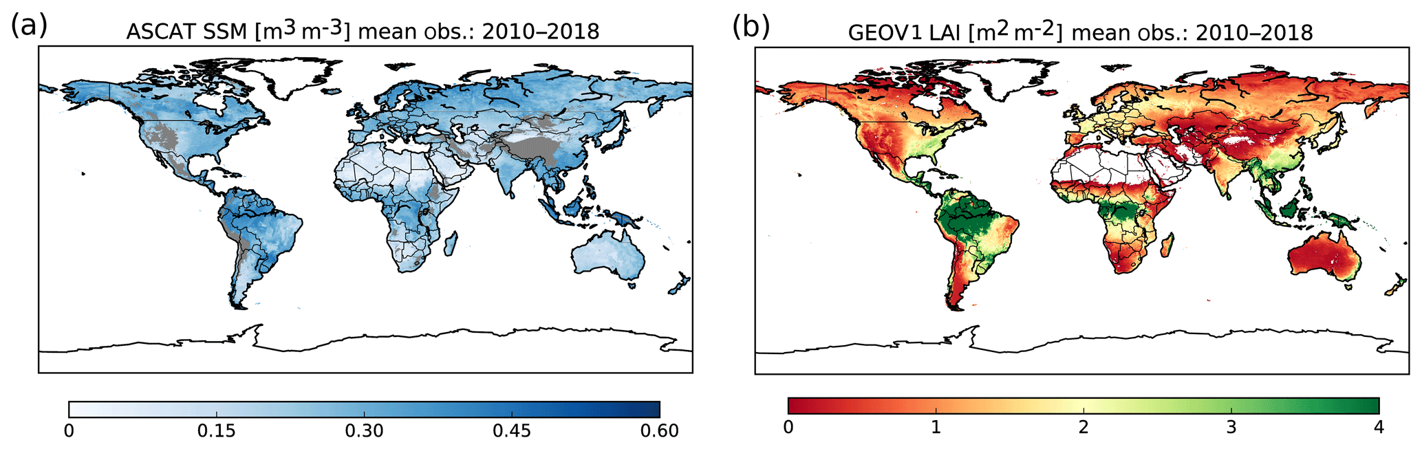
Figure 1 (a) Surface soil moisture (SSM) from the Copernicus Global Land Service (CGLS) for pixels with less than 15 % of urban areas and with an elevation of less than 1500 m a.s.l. (b) GEOV1 leaf area index (LAI) from CGLS, for pixels covered by more than 90 % of vegetation, averaged over 2010 to 2018. SSM is obtained after rescaling the ASCAT Soil Wetness Index (SWI) to the model climatology; grey areas in (a) represent filtered-out data (see Sect. 2.3).

2.1.2 CTRIP river-routing system

The ISBA-CTRIP river-routing system is able to simulate continental-scale hydrological variables based on a set of three prognostic equations. They correspond to (i) the groundwater, (ii) the surface stream water and (iii) the seasonal floodplains. It converts the runoff simulated by ISBA into river discharge. The ISBA-CTRIP river-routing network has a spatial resolution of 0.5^∘ globally and is coupled daily with ISBA through the OASIS3-LCT coupler (Voldoire et al., 2017). ISBA provides CTRIP with updated fields of runoff, drainage, groundwater and floodplain recharges. In turn, CTRIP provides ISBA with water table depth, floodplain fraction as well as flood potential infiltration. Subsequently, ISBA can simulate capillary rise, evaporation and infiltration over flooded areas. A comprehensive overview of how CTRIP is coupled with ISBA is available in Decharme et al. (2019).

2.1.3 Data assimilation

The SEKF used in LDAS-Monde is a two-step sequential approach in which a prior forecast step is followed by an analysis step. The prior forecast propagates the initial states to the next time step with the ISBA LSM and the analysis step then corrects this forecast by assimilating observations. The flow dependency (dynamic link) between the prognostic variables and the observations is ensured in the SEKF through the observation operator and its Jacobians, which propagate information from the observations to the analysis via finite-difference computations (de Rosnay et al., 2013). The Jacobian matrix has as many rows as assimilated observation types (two in our case: SSM and LAI) and as many columns as model control variables requested (eight in our case, soil moisture from layers 2 to 8 and LAI). In addition to a control run (i.e. the forecast step), computing the Jacobian matrix requires perturbed runs, one for each control variable. The eight control variables are directly updated using their sensitivity to observed variables (i.e. defined by the Jacobian). Other variables are indirectly modified through biophysical processes and feedback from the model. Several studies (e.g. Draper et al., 2009; Rüdiger et al., 2010) have demonstrated that small perturbations lead to a good linear approximation of the model behaviour, provided that computational round-off error is not significant. Typically, for those runs, the initial state of the control variable is perturbed by about 0.1 % (see Albergel et al., 2017; Rüdiger et al., 2010). The length of the LDAS-Monde assimilation window is 24 h. A mean volumetric standard deviation error of 0.04 m³ m⁻³ is prescribed for soil moisture in the second layer of soil (i.e. the model equivalent of the observations, between 1 and 4 cm): it is 0.02 m³ m⁻³ for soil moisture in deeper layers (soil layers 3 to 8, 4–100 cm). Both are then scaled by the dynamic range of soil moisture (the difference between the volumetric field capacity and the wilting point, calculated as a function of the soil type, as given by Noilhan et Mahfouf, 1996). The observational SSM error follows the same approach and a value of 0.05 m³ m⁻³ is used. This is consistent with errors typically expected for remotely sensed SSM (e.g. de Jeu et al., 2008, Gruber et al., 2016). Based on previous results from Jarlan et al. (2008), Rüdiger et al. (2010) and Barbu et al. (2011), observed LAI standard deviation errors are set to 20 % of the LAI value itself. The LAI prior forecast errors are set equivalent to the observation errors for values higher than 2 m² m⁻². For values lower than 2 m² m⁻², a fixed standard deviation error of 0.04 m² m⁻² has been used. More details about this approach can be found in Barbu et al. (2011) (Sect. 2.3 and Fig. 2).

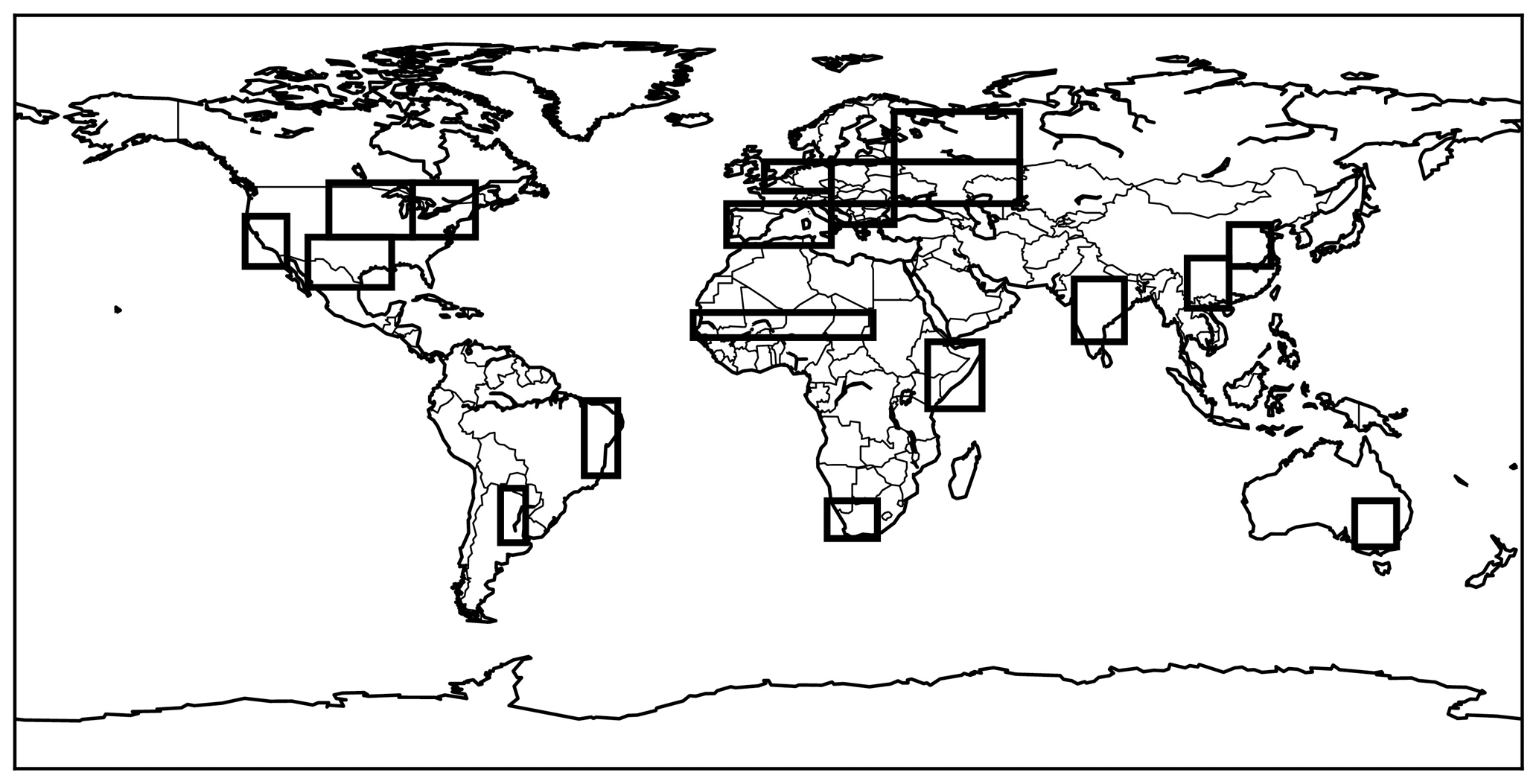
Figure 2 Selection of 19 regions across the globe known for being potential hotspots for droughts and heatwaves. The regions are defined in Table 1.

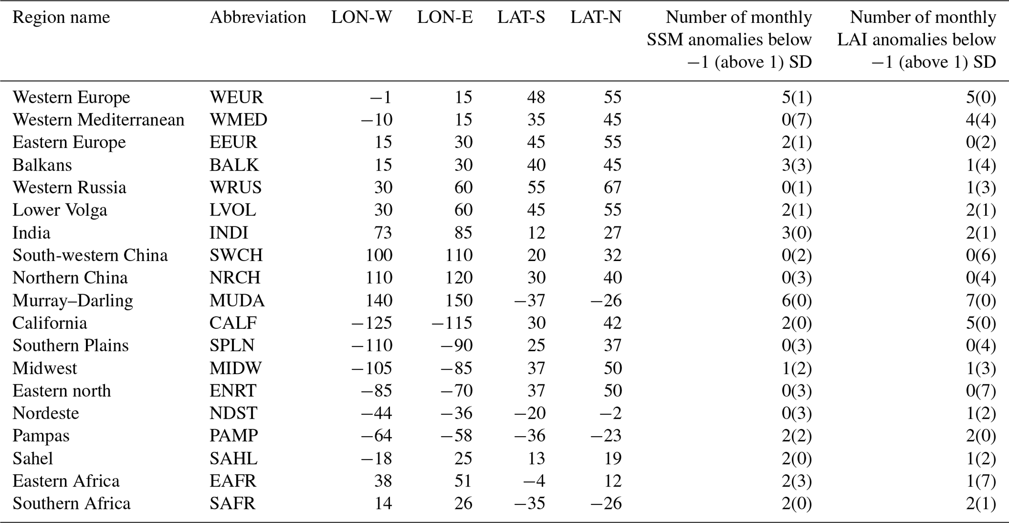
Table 1 Continental hotspots for droughts and heatwaves and number of monthly anomalies SSM and LAI below −1 standard deviation (SD) and above 1 SD in 2018 with respect to the 2010–2018 period.

2.2 Atmospheric forcing

The lowest level of the atmospheric model (about 10 m a.g.l.) of air temperature, wind speed, specific humidity and pressure, the downwelling fluxes of shortwave and longwave radiations as well as precipitation (partitioned into solid and liquid phases) are needed to force LDAS-Monde. In this study, LDAS-Monde is driven by several near-surface meteorological fields from the ECMWF:

• its most recent atmospheric reanalysis (ERA5) to produce an LDAS-Monde global reanalysis;

• its high-resolution Integrated Forecast System (IFS HRES) to monitor and predict the evolution of LSVs for regions under severe droughts and heatwaves.

ERA5 (Hersbach et al., 2018, 2020) is the fifth generation of global reanalyses produced by the ECWMF. This atmospheric reanalysis is a key element of the Copernicus Climate Change Service (C3S) and is available from 1979 onward (data are released about 2 months behind real time). ERA5 produces analyses at an hourly output and at 31 km horizontal resolution and consists of 137 levels in the vertical. Several studies have validated the ERA5 dataset. For example, Urraca et al. (2018) have compared incoming solar radiation from both ERA5 and the ERA-Interim reanalysis (Dee et al., 2011) at a global scale and found evidence that ERA5 outperforms ERA-Interim. In another study, Beck et al. (2019) have highlighted the good performance of ERA5 precipitation with respect to a set of 26 gridded (sub-daily) precipitation data sources by comparing them to Stage-IV gauge-radar data over the CONUS domain (CONtinental United States of America). Tall et al. (2019) have used in situ measurements of precipitation at more than 100 stations spanning all over Burkina Faso in western Africa as well as incoming solar radiation from four in situ stations. They evaluated the performance of ERA5 compared to ERA-Interim and found improved results for ERA5 as well. Furthermore, they evaluated both reanalysis datasets for their ability to force the ISBA LSM, which demonstrates a clear advantage for ERA5 in terms of the performance of LSVs. Albergel et al. (2018a) made similar comparisons of the ISBA LSM forcing over North America. They showed enhanced performances in the representation of evapotranspiration, snow depth, soil moisture and river discharge for ERA5 relative to ERA-Interim.

At the time of writing, the ERA5 model and data assimilation system (cycle 41r2 of the ECMWF IFS) are very similar to that of the operational weather forecast, HRES, which has production cycles ranging from 41r2 to 45r1 during the study period (more information at https://www.ecmwf.int/en/forecasts/documentation-and-support/changes-ecmwf-model, last access: July 2019). The main difference between ERA5 and HRES over the considered period is the horizontal resolution, consisting of 9 km in HRES and 31 km in ERA5. The atmospheric forcing is interpolated from the native grids of ERA5 and HRES to regular grids at 0.25^∘ and 0.1^∘ respectively, using a bilinear interpolation from the native grid to the regular grid. ERA5 and HRES were used in Albergel et al. (2019) to force LDAS-Monde in order to study the impact of the 2018 summer heatwave in Europe. Authors have highlighted that the HRES configuration (LDAS_HRES hereafter) exhibits better monitoring skills than the coarser-resolution ERA5 configuration.

In forecasting mode, the HRES forecast is also available daily from 00:00 UTC with a 10 d lead time. The HRES forecast step frequency is hourly up to time step 90 (i.e. day 3), 3-hourly from time steps 90 to 144 (i.e. day 6) and 6-hourly from time steps 144 to 240 (i.e. day 10). In the forecast experiments in this study (see Sect. 2.4 for details on the experimental setup) HRES forecasts with a 10 d lead time are used to force the LSM forecasts of the LSVs. By comparing LDAS_HRES open-loop and analysis configurations it is possible to evaluate the impact of the initialisation on the forecast of LSVs. The original 3-hourly time steps are used up to day 6 (time step 144). The 6-hourly time steps from days 6 to 10 are interpolated to 3-hourly frequency to avoid discontinuities.

2.3 Assimilated satellite Earth observations

Two types of satellite-derived variables are assimilated in LDAS-Monde: ASCAT soil water index (SWI) and LAI GEOV1. They are both freely available through the Copernicus Global Land Service (CGLS, https://land.copernicus.eu/global/index.html, last access: June 2019).

ASCAT stands for Advanced Scatterometer, which is an active C-band microwave sensor that is onboard the European MetOp polar orbiting satellites (METOP-A from 2006, -B from 2012 and also -C from 2019). From ASCAT radar backscatter coefficients, it is possible to derive information on SSM following a change detection approach (Wagner et al., 1999; Bartalis et al., 2007). The recursive form of an exponential filter (Albergel et al., 2008) is then applied to estimate the SWI using a timescale parameter, T (varying between 1 and 100 d). T is a surrogate parameter for all the processes potentially affecting the temporal dynamics of soil moisture, including soil hydraulic properties, soil layer thickness, evaporation, runoff and vertical gradient of soil properties. The obtained SWI then ranges between 0 (dry) and 100 (wet). In this study, CGLS SWI-001 (produced with a T value of 1 d) is used as a proxy for SSM (Kidd et al., 2013). Grid points with an average altitude exceeding 1500 m a.s.l. as well as those with more than 15 % of urban land cover are rejected as those conditions are known to inhibit the retrieval of SSM from space. Prior to the assimilation, SSM has to be converted from the observation space to the model space. This is done through a linear rescaling as proposed by Scipal et al. (2007), where the mean and variance of observations are matched to the mean and variance of the modelled soil moisture from the second layer of soil (1–4 cm depth). In practice, the rescaling gives similar results to CDF (cumulative distribution function) matching. The linear rescaling is performed on a seasonal basis (with a 3-month moving window) as suggested by Draper et al. (2011) and Barbu et al. (2014).

The LAI GEOV1 observations are based on data from both SPOT-VGT (up to 2014) and PROBA-V (from 2014) satellites. They span from 1999 to present, have 1 km spatial resolution and are produced according to the methodology developed by Baret et al. (2013). LAI GEOV1 observations have a temporal frequency of 10 d at best and no observations are available during cloudy conditions. LAI data are masked in the presence of modelled snow by the ISBA LSM.

As in previous studies (e.g. Barbu et al., 2014; Albergel et al., 2019), observations are interpolated by an arithmetic average to the model grid points (0.25^∘ or 0.10^∘ in this study) if at least 50 % of the model grid points are observed (i.e. half the maximum amount). ASCAT SSM and LAI GEOV1 are illustrated by Fig. 1.

2.4 Experimental setup

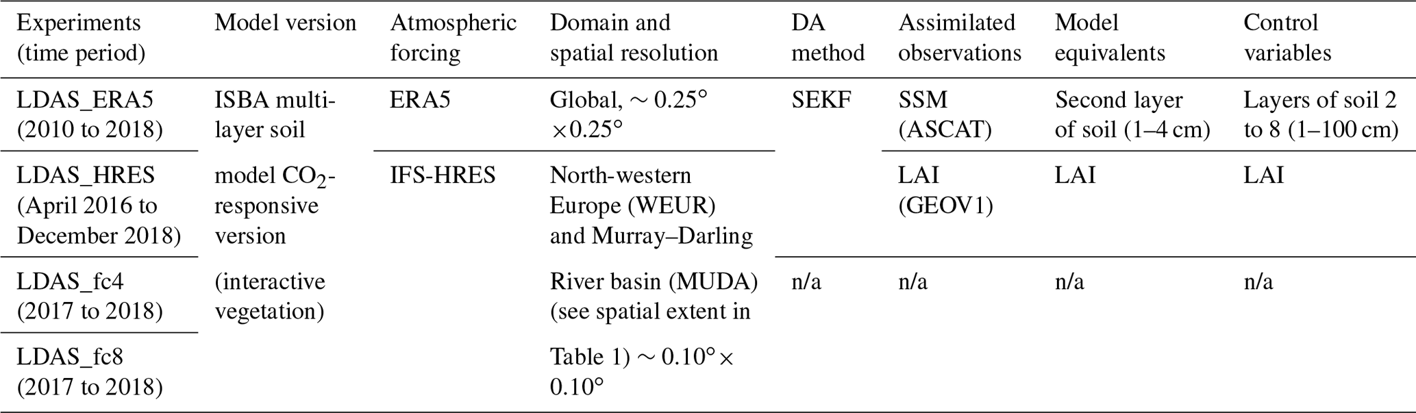
LDAS-Monde is first run globally, at 0.25^∘ spatial resolution, forced by the ERA5 atmospheric reanalysis. It assimilates both SSM and LAI EOs from 2010 to 2018 (LDAS_ERA5). LDAS_ERA5 is spun up by running the year 2010 20 times. The LDAS_ERA5 analysis and its model counterpart (open-loop, i.e. no data assimilation) are presented and evaluated in this study.

This 9-year global reanalysis is then used to provide a monthly climatology for estimating anomalies of the land surface conditions. For each month (and variable considered) of 2018 we have removed the monthly mean and scaled by the monthly standard deviation of the 2010–2018 period. Significant anomalies are used to trigger more detailed monitoring and forecasting activities for a region of interest. A total of 19 regions across the globe have been selected, which are known for being potential hotspots for droughts and heatwaves. They are listed in Table 1 and presented in Fig. 2. Monthly anomalies of SSM and LAI in the LDAS_ERA5 analysis are calculated for 2018 (with respect to the 2010–2018 period) over these 19 regions. In turn, regions presenting significant levels of negative anomalies are selected and further investigated. For those regions, a new LDAS-Monde experiment was driven by the HRES atmospheric analysis, leading to a 0.1^∘ analysis of the LSVs from April 2016 to December 2018 (LDAS_HRES). Note that HRES is only available at a 0.1^∘ spatial resolution from April 2016. April to December 2016 is used as a short period for spin-up and results are presented for the period 2017–2018. Although a 9-month spin-up period is rather short, evaluating LDAS_HRES over either 2017–2018 or 2018 (using instead a 21-month spin-up) leads to similar results on surface soil moisture and LAI (not shown). While the system is not fully spun up, it is long enough to capture the system response to data assimilation. LDAS_HRES complements the coarser spatial resolution LDAS_ERA5.

HRES forecasts with a 10 d lead time are initialized either from LDAS_HRES analysis or open-loop experiments (LDAS_Fc hereafter) in order to assess the impact of the initialization on the forecast. For simplicity, only forecasts with a 4 and 8 d lead time are presented (LDAS_fc4 and LDAS_fc8 respectively). A summary of the experimental setup is given in Table 2.

Table 2 Setup of the experiments performed in this study. LDAS_ERA5 and LDAS_HRES have an analysis (assimilation of surface soil moisture, SSM, and leaf area index, LAI) and a model equivalent (open-loop, no assimilation); LDAS_fc4 and LDAS_fc8 are model runs initialized by either LDAS_HRES open-loop or analysis. n/a stands for not applicable.

2.5 Evaluation datasets and metrics

Both satellite-derived estimates of EOs and in situ measurements are used as reference datasets in this study. The LDAS_ERA5 analysis performance is assessed with respect to the open-loop model run (i.e. no assimilation). The two assimilated datasets, CGLS SSM and LAI, are firstly used to verify that the data assimilation is behaving as expected. Then several independent datasets are used for the validation, namely evapotranspiration from the GLEAM project (Miralles et al., 2011; Martens et al., 2017, version 3b, entirely satellite driven), GPP from the FLUXCOM project (Tramontana et al., 2016; Jung et al., 2017), SIF from the GOME-2 (Global Ozone Monitoring Experiment-2) scanning spectrometer (Munro et al., 2006; Joiner et al., 2016) and snow-cover data from the Interactive Multi-sensor Snow and Ice Mapping System (IMS, https://www.natice.noaa.gov/ims/, last access: August 2020). The IMS snow-cover product combines ground observations and satellite data from microwave and visible sensors (using geostationary and polar-orbiting satellites) to provide snow-cover information in all weather conditions. The IMS product is available daily for the Northern Hemisphere.

Soil moisture is validated using in situ measurements of soil moisture from the ISMN, a pool of stations which consists of 19 networks across 14 countries (see Table S3 in the Supplement). In total, 782 stations are represented with at least 2 years of daily data over 2010–2018. In situ measurements at 5 cm depth (SSM) are compared with soil moisture from the third layer of soil (4–10 cm) in LDAS_ERA5. In situ measurements at 20 cm depth are compared with LDAS_ERA5 soil moisture from the fourth layer of soil (10–20 cm, 685 stations from 10 networks). Besides 11 stations located in four countries of western Africa (Benin, Mali, Sénégal and Niger) and 21 stations in Australia, most of the stations are located in North America and Europe (see Table S3).

Evaluation datasets are listed in Table 3 along with the metrics used for the evaluation. For satellite datasets of SWI, LAI, evapotranspiration and GPP, the metrics consist of the correlation coefficient (R), root mean square difference (RMSD) and normalized RMSD (N_RMSD, Eq. 1).

$$\begin{array}{}\text{(1)}& {\text{N}}_{\mathrm{RMSD}}={\displaystyle \frac{{\mathrm{RMSD}}_{\left(\text{Analysis}\right)}-{\mathrm{RMSD}}_{\left(\mathrm{Model}\right)}}{{\mathrm{RMSD}}_{\left(\mathrm{Model}\right)}}}\times \mathrm{100}\end{array}$$

Regarding the SIF satellite dataset, fluorescence is not simulated directly in the ISBA LSM. However, photosynthesis activity is simulated through the calculation of the GPP, which is driven by plant growth and mortality in the model. Modelled GPP values are expressed in g(C) m⁻² d⁻¹, while SIF is an energy flux emitted by the vegetation (mW m⁻² sr⁻¹ nm⁻¹). Hence, GPP and SIF cannot be directly compared as they do not represent the same physical quantities. However, several studies (e.g. Zhang et al., 2016; Sun et al., 2017; Leroux et al., 2018) have found a high correspondence in both time and space between those two variables, highlighting the potential of SIF products to support the validation of modelled GPP. Therefore, the correlation between modelled GPP and observed SIF is used as an evaluation metric. Concerning the snow-cover dataset, differences between observed and modelled snow cover are considered for the evaluation.

For in situ datasets of soil moisture and evapotranspiration, the standard metrics are considered, namely the correlation coefficient, RMSD, unbiased RMSD and bias. Moreover, a normalized information contribution (NIC, Eq. 2) measure is applied to the correlation values to quantify the improvement or degradation due to the specific configuration.

$$\begin{array}{}\text{(2)}& {\mathrm{NIC}}_R={\displaystyle \frac{R_{\left(\mathrm{Analysis}\right)}-R_{\left(\mathrm{Model}\right)}}{\mathrm{1}-R_{\left(\mathrm{Model}\right)}}}\times \mathrm{100}\end{array}$$

NIC scores are classified according to three categories: (i) negative impact from the analysis with respect to the open-loop with values smaller than −3 %, (ii) positive impact from the analysis with respect to the open-loop with values greater than +3 % and (iii) neutral impact from the analysis with respect to the open-loop with values between −3 % and 3 %.

In addition, for surface soil moisture, the correlation is calculated for both absolute (R) and anomaly (R_anomaly) time series in order to remove the strong impact from the SSM seasonal cycle (see e.g. Albergel et al., 2018a, b).

The Nash–Sutcliffe efficiency score (NSE, Nash and Sutcliffe, 1970, Eq. 3) is used to evaluate LDAS_ERA5 experiments' ability to represent the monthly discharge dynamics.

$$\begin{array}{}\text{(3)}& \mathrm{NSE}=\mathrm{1}-{\displaystyle \frac{\sum _{\mathrm{mt}=\mathrm{1}}^T{\left(Q_s^{\mathrm{mt}}-Q_{\mathrm{o}}^{\mathrm{mt}}\right)}^{\mathrm{2}}}{\sum _{\mathrm{mt}=\mathrm{1}}^t{\left(Q_s^{\mathrm{mt}}-\stackrel{\mathrm{‾}}{Q_s^{\mathrm{mt}}}\right)}^{\mathrm{2}}}},\end{array}$$

where $Q_s^{\mathrm{mt}}$ is the monthly river discharge from LDAS_ERA5 (analysis or open-loop) at month mt, and $Q_{\mathrm{o}}^{\mathrm{mt}}$ is the observed river discharge at month mt. NSE can vary between −∞ and 1. An exact match between model predictions and observed data is defined as a value of 1, whereas a value of 0 means that the model predictions have the same accuracy as the mean of the observed data. Finally, negative values represent situations where the observed mean is a better predictor than the model simulation. NIC presented in Eq. (1) has also been applied to NSE scores to assess the added value of LDAS_ERA5 analysis over its open-loop counterpart. Stations with NSE values less that −2 have been discarded. A similar threshold has already been used in previous studies evaluating LDAS-Monde (e.g. Albergel et al., 2017, 2018a). Many anthropogenic processes are not yet represented in ISBA, including water management from dams and reservoirs, irrigation, and water uptake in urban areas. This could lead to a poor representation of river discharges in those regions. As with previous studies it has been decided to exclude these areas by focusing on stations with reasonable NSE values.

Table 3 Evaluation datasets and associated metrics used in this study. All URLs in this table were last accessed in August 2020.

3 Global assessment of LDAS_ERA5

3.1 Gridded datasets

In this section, the LDAS-Monde open-loop and analysis are firstly compared against the assimilated observations (SSM and LAI) to demonstrate that the assimilation system is working as intended. Both experiments are also compared with independent sources of information to evaluate the analysis impact (GPP, EVAP and SIF).

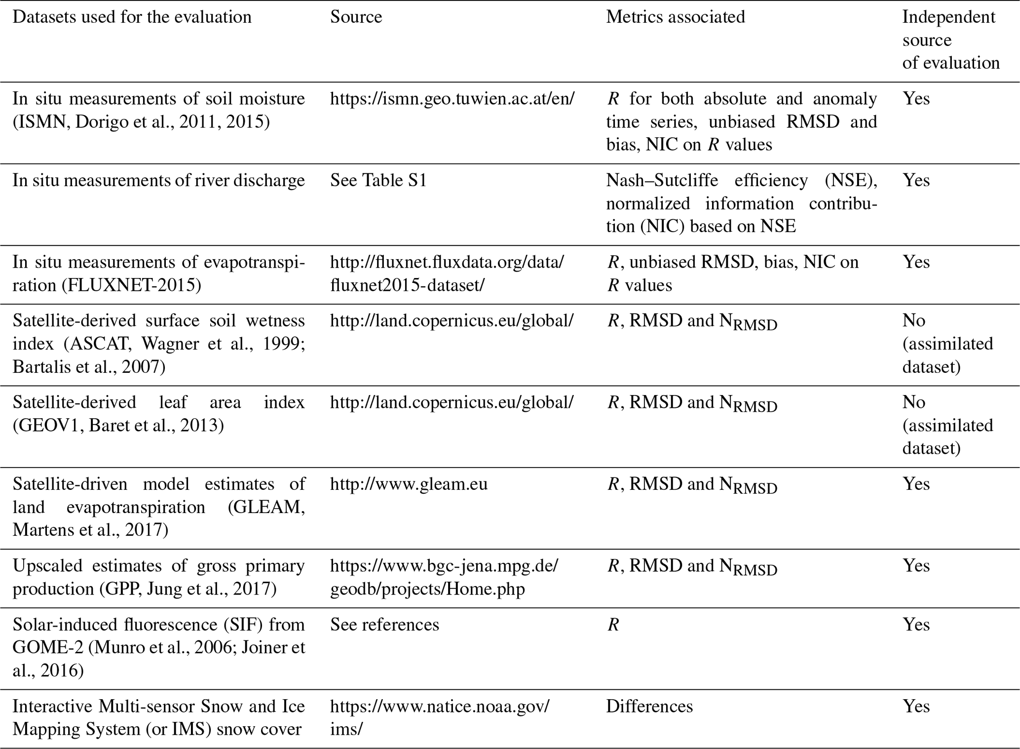
Figure 3 presents mean LAI RMSD values between the observations and LDAS_ERA5 for the open-loop (Fig. 3a) and for the analysis (Fig. 3b) over 2010–2018. Because LAI observations are ingested into the model, the assimilation reduces the LAI RMSD values almost everywhere. It should be noted that rather large LAI RMSD values (>1.5 m² m⁻²) can remain in some areas after the assimilation, especially in densely forested areas.

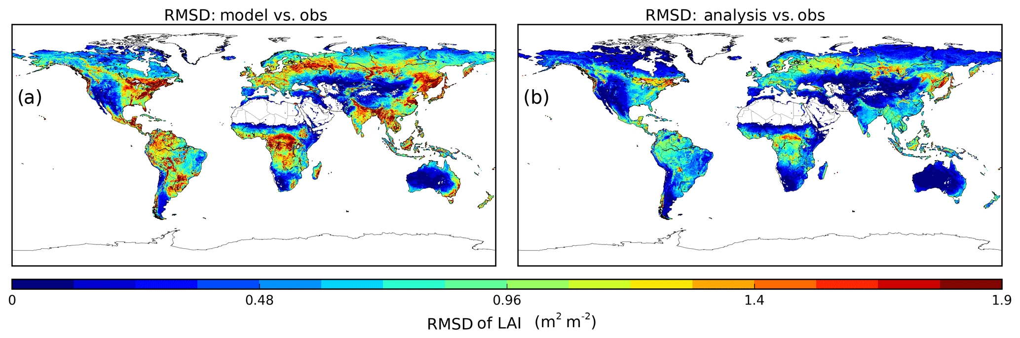
Figure 3 RMSD values between observed leaf area index (LAI) and LDAS_ERA5 (a) before assimilation and (b) after assimilation of surface soil moisture (SSM) and LAI.

Figure 4 illustrates latitudinal plots of LAI, SSM, GPP and EVAP for LDAS_ERA5 before assimilation (the open-loop) and after assimilation (the analysis) along with observations. The number of points considered per 0.25^∘ stripe is also represented. From Fig. 4a it is possible to see the positive impact the analysis has on LAI compared to the open-loop, with the former being closer to the observations. Improvements in the analysis fit are visible between nearly 80^∘ N and about 55^∘ S, and areas around the Equator are impacted the most from the assimilation. This demonstrates that the data assimilation system is working as intended. A smaller impact is obtained for SSM, GPP and EVAP relative to LAI, which is hardly visible at this scale. The mean latitudinal results show a consistent difference in terms of GPP and EVAP between LDAS_ERA5 and the observational products. These differences are systematic with higher values in tropical regions.

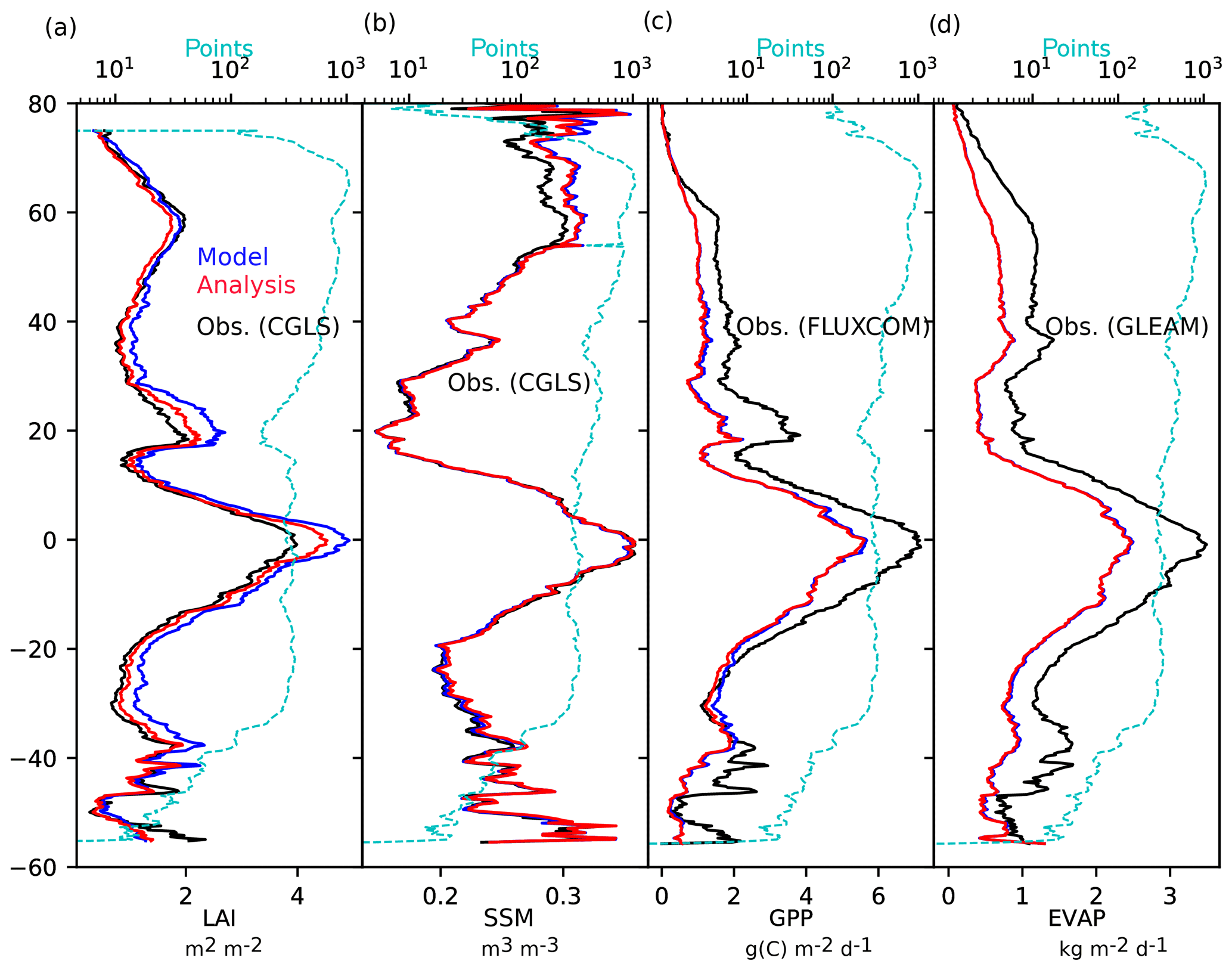
Figure 4 Latitudinal plots of (a) leaf area index (LAI), (b) surface soil moisture (SSM), (c) gross primary production (GPP) and (d) evapotranspiration (EVAP) for LDAS_ERA5 before assimilation (model, blue solid line) and after assimilation (analysis, red solid line) as well as observations (black solid line). Cyan dashed line represents the number of points considered per latitudinal stripe of 0.25^∘.

Figure 5 presents latitudinal plots of score differences (correlations and N_RMSD) for LAI, SSM, GPP, EVAP and SIF. For SIF, it only makes sense to show the correlation differences, since this metric is used to evaluate GPP variability as in Leroux et al. (2018). Score differences are computed by subtracting the open-loop from the analysis. Monthly averages are calculated over 2010–2018 for LAI and SSM, 2010–2013 for GPP, 2010–2016 for EVAP and 2010–2015 for SIF. For each panel of Fig. 5, the vertical dashed line represents the 0 value. For plots of correlation differences, positive values indicate an improvement in the analysis with respect to the open-loop simulation. Similarly, for plots of RMSD differences, negative values indicate an improvement in the analysis with respect to the open-loop simulation. Given that LAI and SSM are assimilated variables, the analysis leads to a clear improvement in both correlation and RMSD. Such an improvement is expected and reflects the healthy behaviour of the assimilation system. Both variables are improved at almost all latitudes, with the exception around 45^∘ S for LAI correlation values (very few land points). For SSM a noticeable improvement in both correlation and RMSD is found around 20^∘ N, which corresponds mainly to an improvement in the Sahara (not shown). Being linked to LAI, GPP is also improved across almost all latitudes (to a lesser extent than LAI), with a particularly positive impact below 20^∘ N. As seen in Fig. 5d and i, there is a negligible impact of the assimilation on EVAP. It highlights the difficulty of land surface data assimilation in impacting model fluxes by modifying model states.

Figure 5 Latitudinal plots of score differences (analysis minus open-loop) for correlations (a–e) and normalized RMSD (f–i) for LAI (a, f), SSM (b, g), GPP (c, h), EVAP (d, i) and SIF (e, correlations only). Scores are computed based on the monthly average over 2010–2018 for LAI and SSM, 2010–2013 for GPP, 2010–2016 for EVAP and 2010–2015 for SIF. Dashed lines represent the zero lines (equal scores for open-loop and analysis).

The panels of Fig. 6 illustrate histograms of score differences (correlation and RMSD, analysis minus open-loop) for LAI, SSM, GPP, EVAP and SIF. The number of available data and the percentage of positive and negative values are reported. For correlations (RMSD) differences, positive (negative) values indicate an improvement in the analysis relative to the open-loop. Regarding LAI, the analysis improves 96.9 % of the grid points for correlations and 99.9 % for N_RMSD. As for SSM, correlation values are improved for 92.8 % of the grid points (92.4 % for RMSD). The independent GPP and SIF datasets also demonstrate improvements in the analysis relative to the open-loop. Indeed, the GPP correlation (RMSD) is better for 81.1 % (74.1 %) of the grid points and the SIF correlation is enhanced for 79.7 %. Results using the GLEAM dataset for evapotranspiration are more contrasting with 63.6 % (48.9 %) of the grid points showing an improvement from the analysis. It is worth mentioning that 24.9 % (39.6 %) of the grid point shows a decrease in skill. However, GLEAM is an evaporation model designed to be driven by remote sensing observations only. GLEAM only estimates (root-zone) soil moisture and terrestrial evaporation, while the CO₂-responsive version of ISBA in LDAS_ERA5 is a physically based land surface model, accounting for more processes linked to vegetation (see Sect. 2.1.1). It should be noted that the auxiliary datasets used to represent the different land cover types also differ. Within GLEAM, the land cover types are sourced from the Global Vegetation Continuous Fields product (MOD44B), based on observations from the Moderate Resolution Image Spectroradiometer (MODIS). Four land cover types are considered, namely bare soil, low vegetation (e.g. grass), tall vegetation (e.g. trees), and open water (e.g. lakes). In ISBA, the fraction of the 12 land cover types over some areas departs from prevalent land cover products such as CLC2000 (Corine Land Cover) and GLC2000 (Global Land Cover). It could potentially impact the distribution of the terrestrial evaporation between GLEAM and ISBA. Further work at CNRM will focus on understanding the differences between ISBA and GLEAM, in particular investigating the sub-components of terrestrial evaporation.

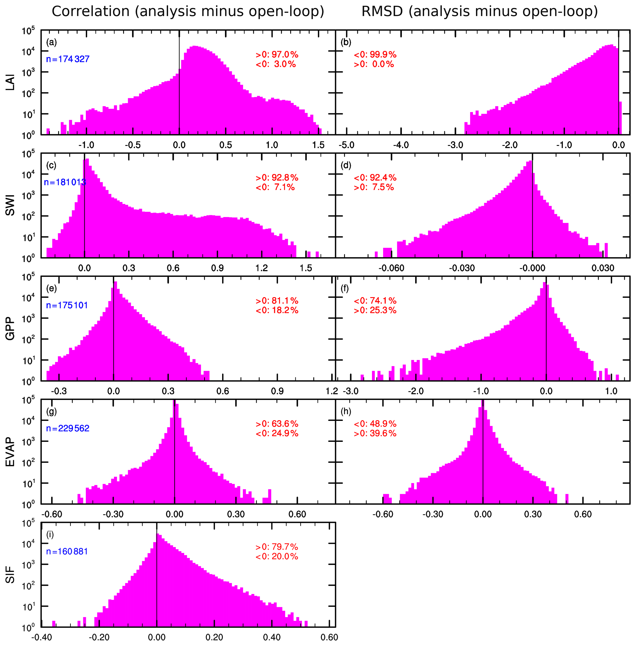
Figure 6 Histograms of score differences (correlation and RMSD, analysis minus open-loop) for (a, b) LAI, (c, d) SSM, (e, f) GPP, (g, h) EVAP and (i) SIF. For SIF only differences in correlation are represented. Number of available data (in blue) as well as the percentage of positive and negative values (in red) are reported. Note that for the sake of clarity, the y axis is logarithmic.

Finally, Figs. S1 and S2 illustrate snow-cover evaluation. LDAS_ERA5 snow cover is evaluated against the IMS snow cover. Fig. S1 shows the averaged Northern Hemisphere snow-cover fraction for the 2010–2018 period. It is complemented by Fig. S2, which shows (i) maps of IMS snow cover (top row) for three seasons, (ii) equivalent maps of snow cover from LDAS_ERA5 open-loop (second row), (iii) maps of snow-cover differences between the open-loop and IMS data and (iv) maps of snow-cover differences between the analysis and the open-loop. LDAS_ERA5 open-loop compares very well with the IMS snow-cover data in the accumulation season from September to February (Figs. S2 and S1d to i), except for an overestimation over the Tibetan Plateau. The issue over Tibet from ERA5 is not new and is consistent with Orsolini et al. (2019). An early melt in spring is visible in LDAS_ERA5 compared to observations and could be related to the snow-cover parametrization in ISBA. As expected, the analysis has an almost neutral impact on snow as both SSM and LAI observations are filtered out during frozen/snow-covered conditions, and there is no snow data assimilation yet in LDAS_ERA5 (Figs. S2 and S1j, k and l). Clearly an area of potential improvement in LDAS-Monde is to incorporate snow data assimilation using satellite data such as IMS (as in e.g. de Rosnay et al., 2014).

3.2 Ground-based datasets

LDAS_ERA5 analysis and open-loop are also evaluated using independent in situ measurements of evapotranspiration, river discharge and surface soil moisture across the world. Daily in situ measurements of evapotranspiration from the FLUXNET-2015 synthesis dataset (http://fluxnet.fluxdata.org/, last access: June 2019) are first used in this study. The LDAS_ERA5 evapotranspiration performance is evaluated using the correlation coefficient (R), RMSD, ubRMSD and the bias (LDAS_ERA5 minus observations) using the 85 selected FLUXNET-2015 stations. The median R, RMSD, ubRMSD and bias for LDAS_ERA5 analysis (open-loop) are 0.73 (0.72), 28.74 (29.60) W m⁻², 27.37 (26.92) W m⁻² and 4.64 (4.40) W m⁻² respectively. Although these values depict a small advantage of the analysis over the open-loop, it is worth mentioning that these differences are rather small and likely to fall within the uncertainty of the in situ measurements.

Figure 7a represents the added value of the analysis based on NIC_R (Eq. 2), the large blue circles represent a positive impact from the analysis (20 stations) with a NIC_R greater than +3 (i.e. R values are better when the analysis is used than when the model is used), while large red circles represent a degradation from the analysis (5 stations) with a NIC_R smaller than −3. Stations with a rather neutral impact (60 stations) have a NIC_R between [−3; +3] and are reported using small dots. Note that at the scale of Fig. 7a, some stations are overlapping. Figure 7a is complemented by panels b, c, d and e which show scatter plots of R, ubRMSD, absolute bias and RMSD between LDAS_ERA5 analysis (x axis) and the open-loop (y axis) for the 85 stations from the Fluxnet2015. Out of the 85 stations considered, 56 have better R values in the analysis compared to the open-loop. The respective numbers of improved stations for ubRMSD, RMSD and the absolute bias equate to 41, 47 and 44 respectively. The set of 20 stations from Fig. 7a where the analysis has a positive impact on the NIC_R (greater than +3) are reported in green in Fig. 7b.

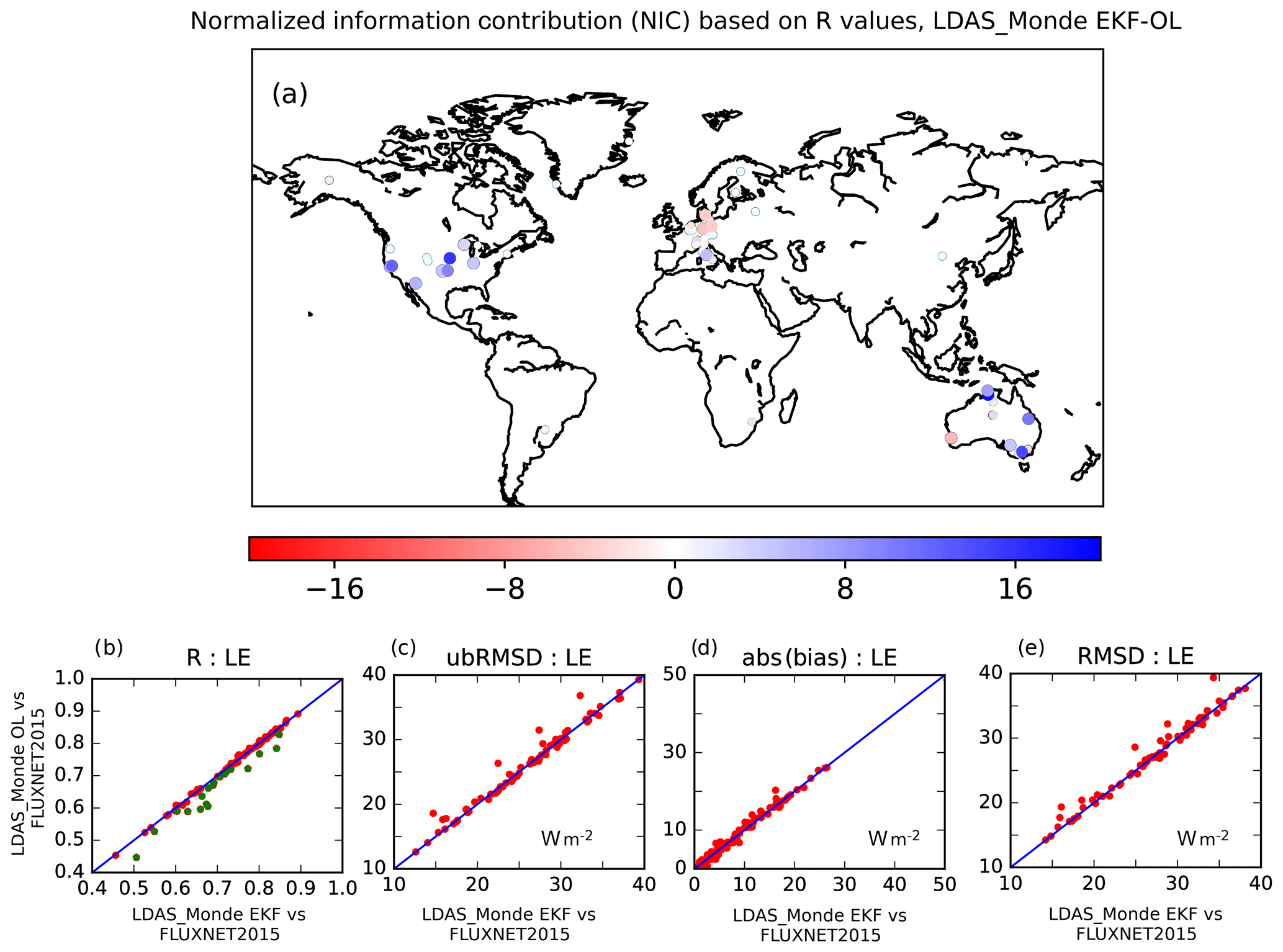
Figure 7 (a) Map of the normalized information contribution (NIC, Eq. 2) applied to correlation values between evapotranspiration from LDAS_ERA5 analysis (open-loop) and observations from the FLUXNET 2015 synthesis dataset. NIC scores are classified into two categories: (i) negative impact from the analysis with respect to the model with values smaller than −3 % (red circles, 5 stations) and (ii) positive impact from the analysis with respect to the model with values greater than +3 % (blue circles, 20 stations). Stations presenting a neutral impact with values between −3 % and +3 % (60 stations) are reported as small dots. Note that at this scale some stations are overlapping. (b, c, d and e) Scatter plots of R, ubRMSD, absolute bias and RMSD between LDAS_ERA5 open-loop and the 85 stations from the FLUXNET 2015 (y axis) and LDAS_ERA5 analysis and the same pool of stations (x axis). The set of 20 stations for which the analysis has a positive impact on R values at NIC_R greater than +3 is reported in (a) in green.

Results on river discharge are illustrated by Fig. 8 (panels a and b). Figure 8a represents NSE scores for the subset of 982 stations selected. Most of them are located in North America and Europe, while a few are available in South America and Africa. Figure 8a is complemented by Fig. 8b, which shows the NIC score applied to the NSE score. It emphasizes the added value of the LDAS_ERA5 analysis over the open-loop. From this subset of stations, 74 % present a rather neutral impact from the analysis (with a NIC ranging between −3 % and +3 %), while 26 % (254 stations) present a significant impact (with a NIC above +3 % or below −3 %). When the analysis significantly impacts the representation of river discharge, this impact tends to be positive. Indeed, 74 % of this subset of stations (189 stations) have a NIC score greater than 3 % while only 26 % (65 stations) show NIC scores smaller than −3 %.

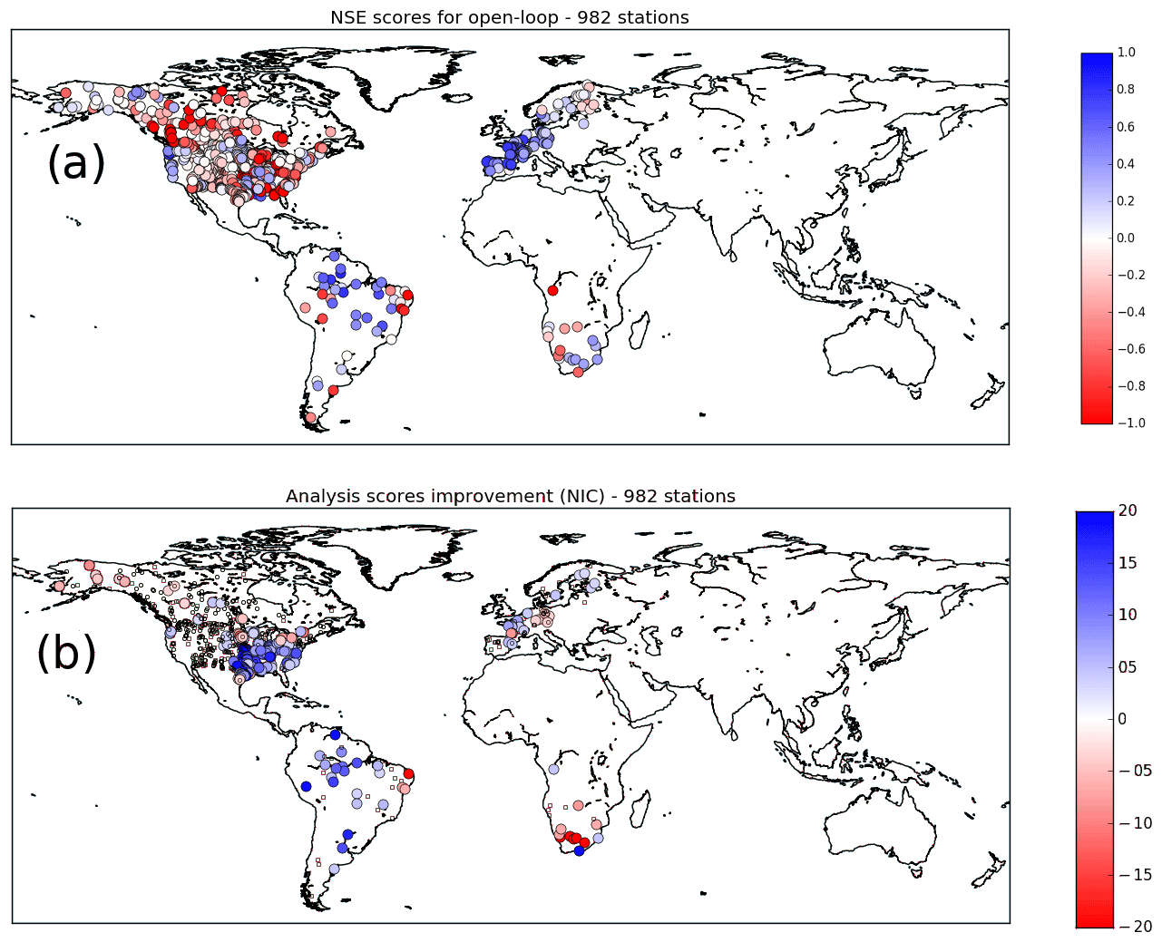
Figure 8 (a) Global map of Nash–Sutcliffe efficiency scores (NSE) between river discharge from LDAS_ERA5 open-loop and in situ measurements from the networks presented in Table S1 over 2010–2016. (b) Normalized information contribution scores (NIC, Eq. 2) based on NSE scores on river discharge. Small dots represent stations for which NICs are between [−3 %, +3 %] (i.e. neutral impact from LDAS_ERA5 analysis), NIC values greater than +3 % (blue large circles) suggest an improvement from LDAS_ERA5 analysis over LDAS_ERA5 open-loop, while values smaller than −3 % (large red circles) suggest a degradation. Only stations where more than 4 years of data are available and with a drainage area greater than 10 000 km² are considered. Stations with NSE values smaller than −2 are discarded, also leading to a subset of 982 stations available.

The statistical scores for soil moisture from LDAS_ERA5 open-loop and analysis are presented for the third and fourth layers of soil, corresponding to 4–10 cm depth and 10–20 cm depth respectively. The soil moisture at layers 3 and 4 is compared with ground measurements over 2010–2018 from the ISMN at depths of 5 and 20 cm respectively. The results are displayed in Table S3 for each individual network. Averaged statistical scores (ubRMSD, R, R_anomaly and bias) are similar for both LDAS_ERA5 analysis and open-loop even if local differences exist. For the analysis, averaged R (R_anomaly) values for the third layer, along with their 95 % Confidence intervals (CIs) (782 stations from 19 networks) are $\mathrm{0.68}\pm \mathrm{0.03}(\mathrm{0.53}\pm \mathrm{0.04})$. For the open-loop, the averaged R (R_anomaly) values are $\mathrm{0.67}\pm \mathrm{0.03}(\mathrm{0.53}\pm \mathrm{0.04})$. Averaged-network values are highest for the SOILSCAPE network with values of $\mathrm{0.88}\pm \mathrm{0.01}(\mathrm{0.58}\pm \mathrm{0.04})$ for the analysis (49 stations in the USA). For all networks, the average R values are higher than 0.55, with the exception of ARM (10 stations in the USA), which presents an averaged R value of 0.29±0.05. Averaged ubRMSD and bias (LDAS_ERA5 minus in situ) are 0.060 and 0.077 m³ m⁻³ for the analysis respectively. The open-loop has a similar performance, with an ubRMSD and bias of 0.060 and 0.076 m³ m⁻³ respectively. NIC (Eq. 2) has also been applied to R values. In total, 65 % of stations present a neutral impact of the analysis compared to the open-loop (511 stations at NIC ranging between −3 and +3), 12 % present a negative impact (91 stations at NIC <−3) and 23 % present a positive impact (180 stations at NIC >+3).

The number of stations where R differences between the analysis and the open-loop are significant (i.e. their 95 % CIs are not overlapping) is 186 out of 782 (about 26 %). There is an improvement from the analysis with respect to the open-loop for 128 stations (about 69 %) and a degradation for 58 stations (about 31 %). Figure 9 illustrates R differences between the analysis and the open-loop runs over CONUS where most of the stations are located (552 out of 782). When differences (analysis minus open-loop) are not significant, stations are represented by a small dot (425 stations out of 552). When they are significant (127 stations out of 552), large circles have been used, with blue corresponding to positive differences (99 stations out of 127) and red to negative differences (28 stations out of 127). For most of the stations where a significant difference is obtained, it represents an improvement from the analysis.

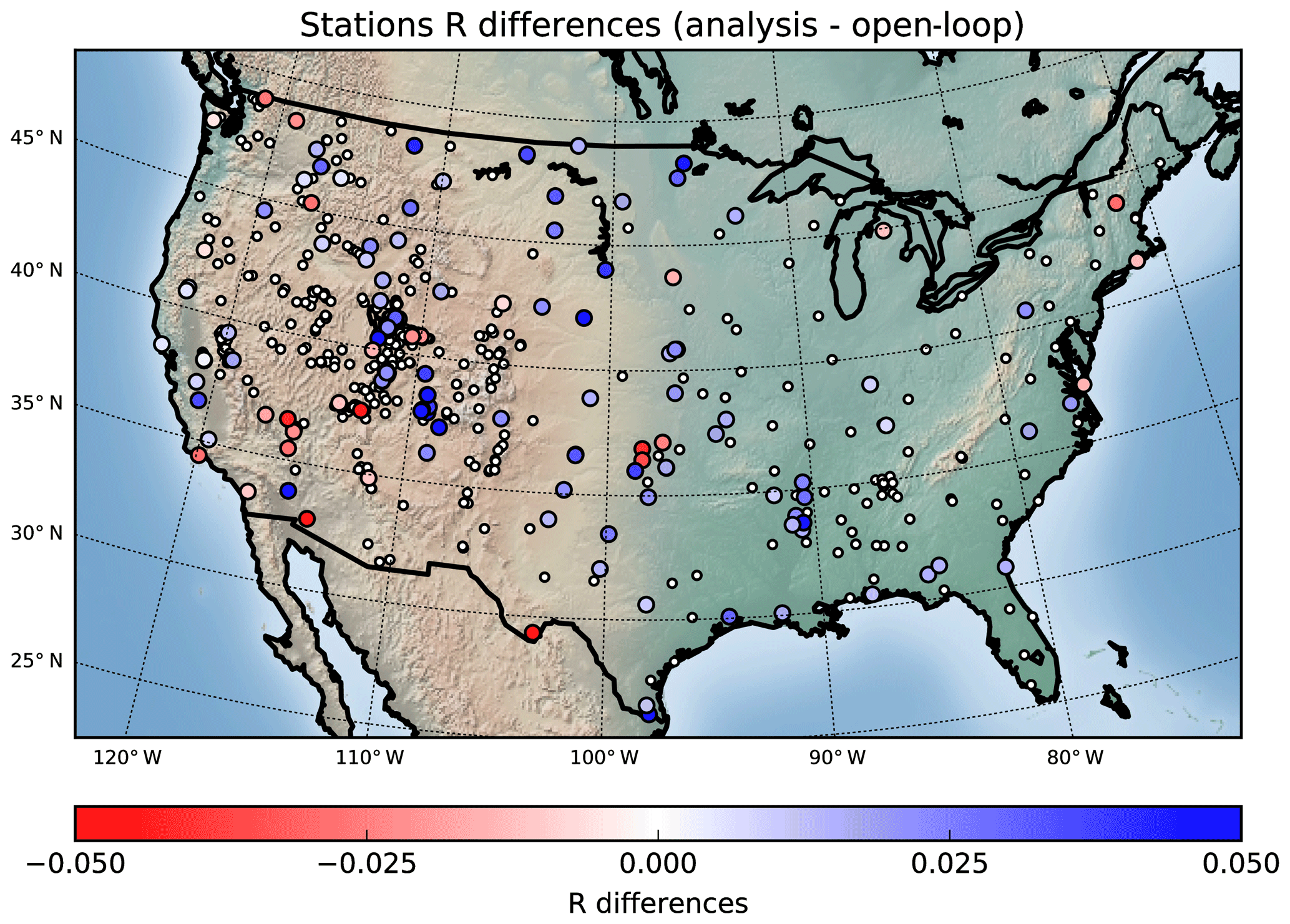
Figure 9 Map of correlation (R) differences (analysis minus open-loop) for stations measuring soil moisture at 5 cm depth and being available over North America. Small dots represent stations where R differences are not significant (i.e. 95 % confidence intervals are overlapping), large circles where differences are significant.

Averaged analysis R (95 %CI), bias and ubRMSD for the fourth layer of soil (685 stations from 10 networks) are 0.65±0.03, 0.049 and 0.055 m³ m⁻³ respectively. For the open-loop, they are 0.64±0.03, 0.048 and 0.056 m³ m⁻³ respectively. In terms of the NIC, about 60 % of the stations demonstrate a neutral impact of the analysis compared with the open-loop, while 28 % show a positive impact and 12 % a negative impact. Although differences between the open-loop run and the analysis are rather small, these results underline the added value of the analysis with respect to the model run. Figure S3 represents the distribution of the scores values for LDAS_ERA5 open-loop and analysis using box plots centred on the median value. It is difficult to see any important differences between them.

For evapotranspiration, river discharge and surface soil moisture there is a slight advantage for the LDAS_ERA5 analysis with respect to its open-loop counterpart. Even if the averaged statistical metrics are rather similar for both, there are significant differences at the regional scale.

4 Monitoring and forecasts for areas under severe/extreme conditions

4.1 Selection of two regional case studies

For each individual region presented in Table 1 and Fig. 2, monthly anomalies (scaled by the standard deviation) of analysed SSM (second layer of soil, 1–4 cm) and LAI for 2018 are assessed with respect to the 2010–2018 average. The anomalies (see Fig. 10) highlight three regions, two of which present strong negative anomalies for both SSM and LAI for almost all of 2018. These are north-western Europe (WEUR) and the Murray–Darling basin (MUDA) in south-eastern Australia. Contrastingly, eastern Africa (EAFR) presents strong positive anomalies of SSM and LAI. WEUR and MUDA regions were affected by a severe heatwave and a drought in 2018, which impacted the LSVs analysed by LDAS_ERA5. According to Fig. 10, monthly anomalies of SSM and LAI for MUDA are negative through 2018, with 7 (6) months presenting LAI (SSM) anomalies below −1 standard deviation (SD) respectively. WEUR has negative SSM anomalies from May to December 2018, with values dipping below −2 SD. LAI was severely impacted as well, with July to October 2018 presenting negative anomalies below −2 SD. For WEUR, 5 months show LAI and SSM anomalies below −1 SD. On the other hand, EAFR experienced 3 (7) months with positive anomalies for SSM and LAI in 2018 above 1 SD.

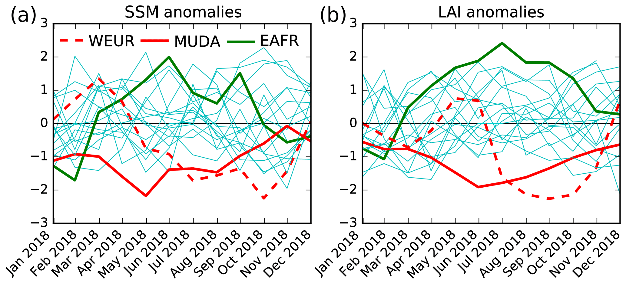
Figure 10 2018 monthly anomalies scaled by standard deviation of analysed (a) SSM and (b) LAI, with respect to 2010–2018, for the 19 regions presented in Table 1 and Fig. 2. Solid red line, dashed red line and solid green line represent regions MUDA, WEUR and EAFR. Solid cyan line represents all other boxes (see Table 1 and Fig. 2).

According to the National Oceanic and Atmospheric Administration (NOAA), Europe experienced its warmest summer since continental records began in 1910 with a positive anomaly at +2.16 ^∘C above mean (Global Climate Report, https://www.ncdc.noaa.gov/sotc/global/, last access: April 2019). In Europe, temperatures over all the summer months in 2018 were above the climatological mean. The summer 2018 heatwave in Europe has already been reported in the scientific literature (e.g. Magnusson et al., 2018; Albergel et al., 2019; Blyverket et al., 2019).

In its 70th Special Climate Statement, the Australian Bureau of Meteorology (BoM) reported a very hot and dry summer 2018 in eastern Australia (BoM, 2019). Like much of Australia, the Murray–Darling basin also experienced remarkably dry and hot weather during 2018. The annual maximum temperature for the Murray–Darling basin as a whole was more than 2^∘ above average during 2018. The northern Murray–Darling basin in particular was severely affected, with inflows to all river catchments persistently well below normal (http://www.bom.gov.au/state-of-the-climate/, last access: April 2019). Finally, the East African Seasonal Monitor based on the Famine Early Warning System Network (FEWS) confirms above-average rainfall amounts and significantly greener-than-normal vegetation conditions (e.g. https://reliefweb.int/report/somalia/east-africa-seasonal-monitor-july-27-2018, last access: April 2019). As this study focuses on monitoring and forecasting the impact of severe drought conditions on LSVs, the WEUR and MUDA regions are selected for further investigation.

4.2 Case studies: LDAS-Monde medium-resolution (0.25^∘) experiments

Figure 11 illustrates seasonal cycles of observed LAI (Fig. 11a) and SWI (Fig. 11e), LDAS_ERA5 analysis and open-loop LAI (Fig. 11b) and SSM (Fig. 11f) for the WEUR domain. The 2018 period is compared to the 2010–2017 average. Figure 11a shows the heatwave impact with a sharp drop in observed LAI values from June to November 2018 (solid green line). Such low LAI values have never been observed over the 8 previous years (it is below the minimum value in shaded green). A similar behaviour is also visible in the ASCAT SWI dataset in Fig. 11e, with the lowest values recorded in 2018 for the 2010–2018 period. Over WEUR, LDAS_ERA5 open-loop overestimates LAI in the second part of the year, as already highlighted by several studies (e.g. Albergel et al., 2017, 2019). The LDAS_ERA5 analysis has a positive impact and reduces LAI values, as seen in Fig. 11b. Figure 11c, d, g and h depict a similar situation for the MUDA area: almost every month of 2018 presents the lowest values for both SSM and LAI. For both MUDA and WEUR, the smaller differences for LAI and SSM between LDAS_ERA5 analysis and open-loop in 2018 indicates that both extreme events were well captured in the atmospheric forcing used to drive LDAS_ERA5.

Figure 11 Upper panels represent seasonal cycles of (a) observed GEOV1 LAI from CGLS and (b) LAI from the open-loop (in blue) and the analysis (in red) for the WEUR area (see Table 1 for geographical extent). Panels (c) and (d) are similar to (a) and (b) for the MUDA area. Lower panels represent seasonal cycles of (e) ASCAT SWI from CGLS and (f) SSM from the open-loop (in blue) and the analysis (in red) for the WEUR area. Panels (g) and (h) are similar to (e) and (f) for the MUDA area. For each panel dashed line represents the average over 2010–2017 along with the minimum and maximum values; the solid lines are for the year 2018.

4.3 Case studies: LDAS-Monde high-resolution (0.1^∘) analysis and forecast experiments

For the two selected areas (WEUR and MUDA), LDAS-Monde is also run over April 2016 to December 2018 with the atmospheric forcing from HRES (LDAS_HRES) at 0.1^∘ spatial resolution. Additionally, daily forecast experiments are performed and the results presented for LAI and SSM for lead times of 4 and 8 d. These forecasts are initialized by either LDAS_HRES analysis or open-loop over 2017–2018 in order to assess the impact of the initial conditions. In this subsection, this new set of six experiments is verified against the assimilated observations. Verification of the forecasts with these observations can be viewed as an independent validation as those observations are not assimilated yet. It is worth mentioning that there is a difference between the use of SSM and LAI observations to evaluate the forecast. For SSM, the assimilation is done after a rescaling of the observations to the model climatology (see Sect. 2.3), which removes bias. However, for LAI this is not the case, and the assimilation process removes the bias in the modelled LAI with respect to the observations. This difference, together with the longer memory of LAI (compared to SSM), contributes to the results presented in this sub-section. Statistical scores for LDAS_HRES open-loop and analysis are also presented, which serve as a benchmark for the forecast experiments.

Figure 12 (for WEUR) and Fig. 13 (for MUDA) upper panels illustrate the seasonal RMSD (Figs. 12a, 13a) and correlation (Figs. 12b, 13b) between LDAS_HRES SSM from the second layer of soil (1–4 cm) and ASCAT SSM estimates over 2017–2018. Scores are also reported for the LDAS_HRES 4 d (LDAS_fc4) and 8 d forecasts (LDAS_fc8). From the upper panels of those figures one may notice a small improvement from the analysis (solid red line) over the open-loop simulation (solid blue line), with slightly reduced RMSD values and increased correlation values. However, no improvement (or degradation) is visible from the 4 and 8 d forecast experiments initialized by LDAS_HRES analysis over those initialized by LDAS_HRES open-loop. As expected, LDAS_HRES SSM is closer to the observations compared with LDAS_fc4 and LDAS_fc8. It is worth pointing out that for the MUDA area there is a small positive impact of the initialization on the 4 and 8 d forecasts of surface soil moisture (Fig. 13a, b). These results suggest that the fast-evolving SSM model variable is more sensitive to the atmospheric forcing than to the initial conditions (at least within the forecast range presented in this study). Results for LAI are different from SSM (Figs. 12c, d and 13c, d). Firstly, there is a large improvement from the analysis (solid red line) over the open-loop (solid blue line), particularly during the LAI decaying phase (boreal and austral autumns mainly). Secondly, the LDAS_HRES open-loop (solid blue line) and the forecasts initialized by the open-loop (LDAS_fc4 and LDAS_fc8) perform similarly. Furthermore, the LDAS_fc4 and LDAS_fc8 forecasts are quite consistent when initialized by the LDAS_HRES analysis. Importantly, the LDAS_HRES analysis and forecasts outperform the LDAS_HRES open-loop initial conditions and forecasts. This suggests that LAI forecasts are more sensitive to initial conditions than to the atmospheric forcing within the 4–8 d range for both WEUR and MUDA regions.

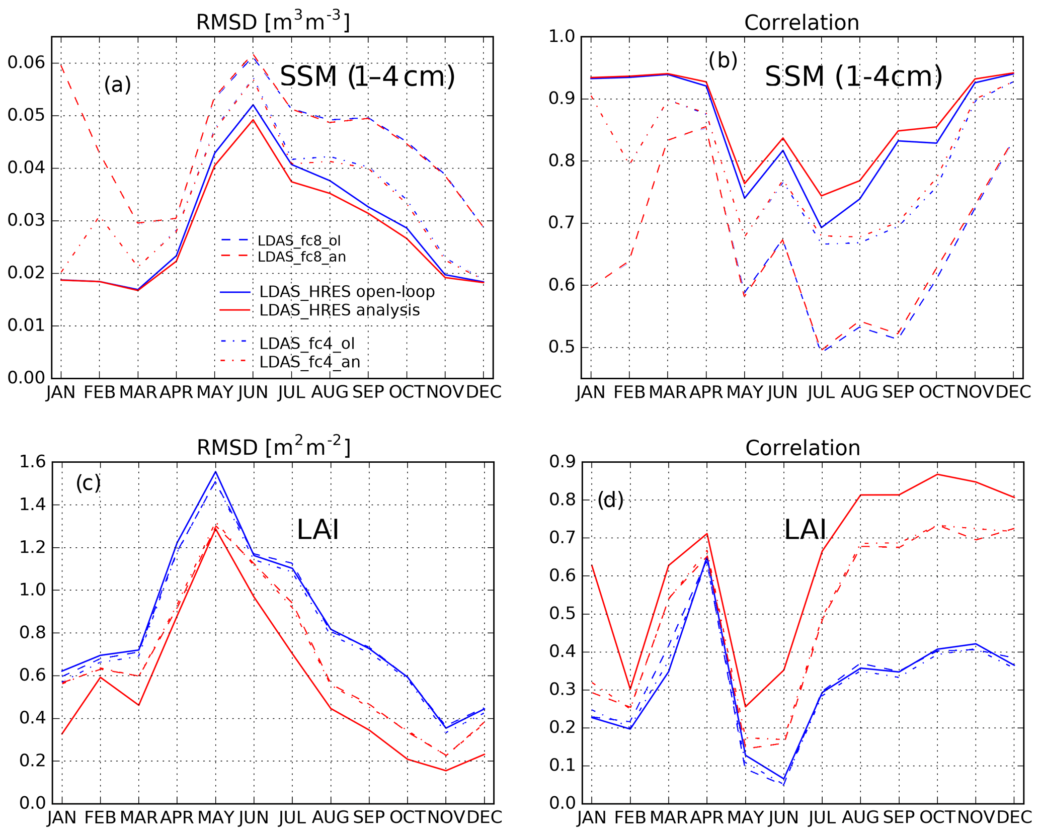
Figure 12 Seasonal (a) RMSD and (b) correlation values between soil moisture from the second layer of soil (1–4 cm) from the model forced by HRES (LDAS_HRES, open-loop in blue solid line, analysis in red solid line) and ASCAT SSM estimates over 2017–2018 over the WEUR area. Scores between SSM from the second layer of soil of LDAS_HRES, 4 d (dashed/dotted blue – when initialized by the open-loop – and red – when initialized by the analysis – lines) and 8 d (dashed blue and red lines) forecasts and ASCAT SSM estimates are also reported. Panels (c) and (d): same as (a) and (b) between modelled/analysed LAI and GEOV1 LAI estimates.

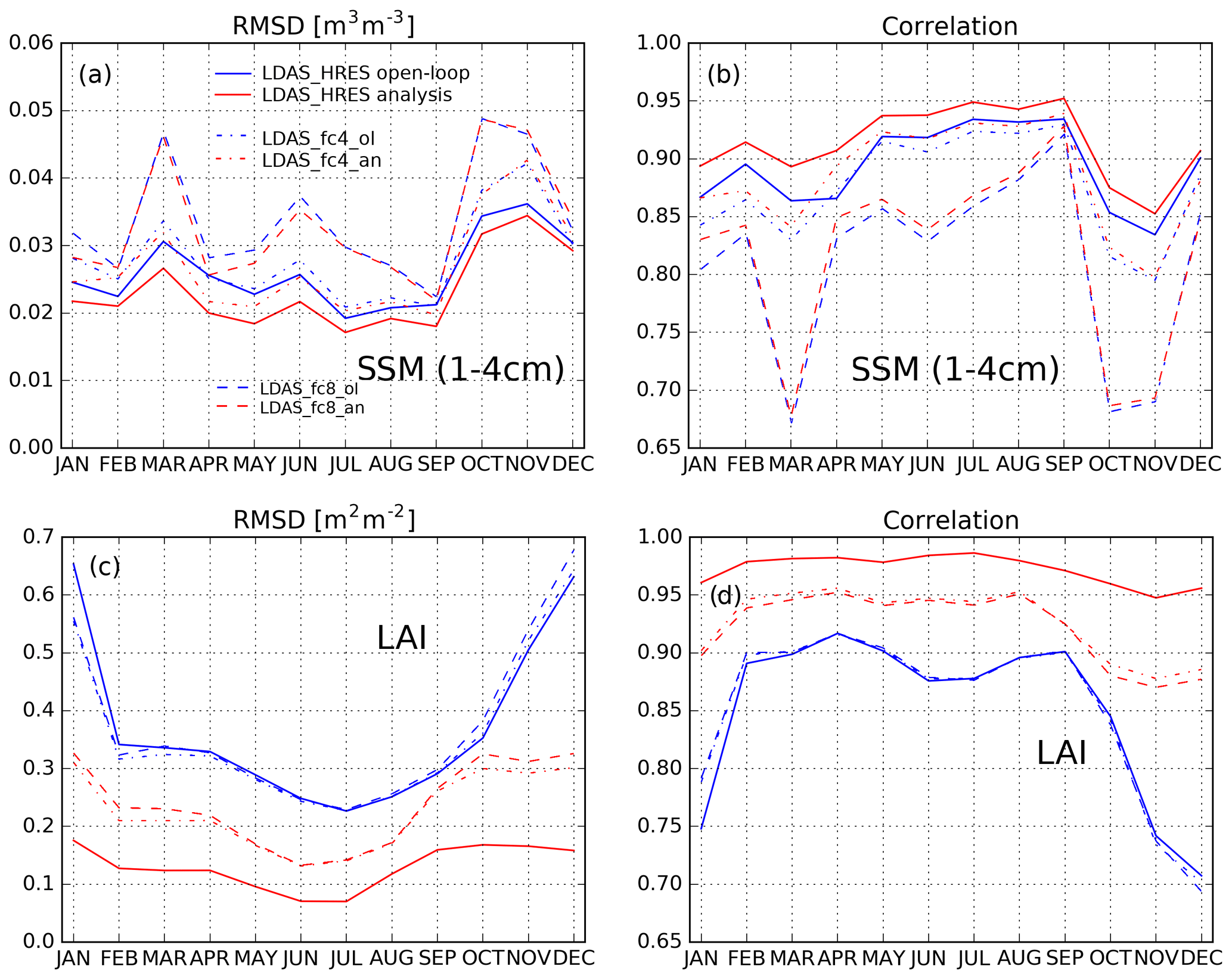
Figure 13 Same as Fig. 12 for the Murray–Darling River (MUDA) area in south-eastern Australia.

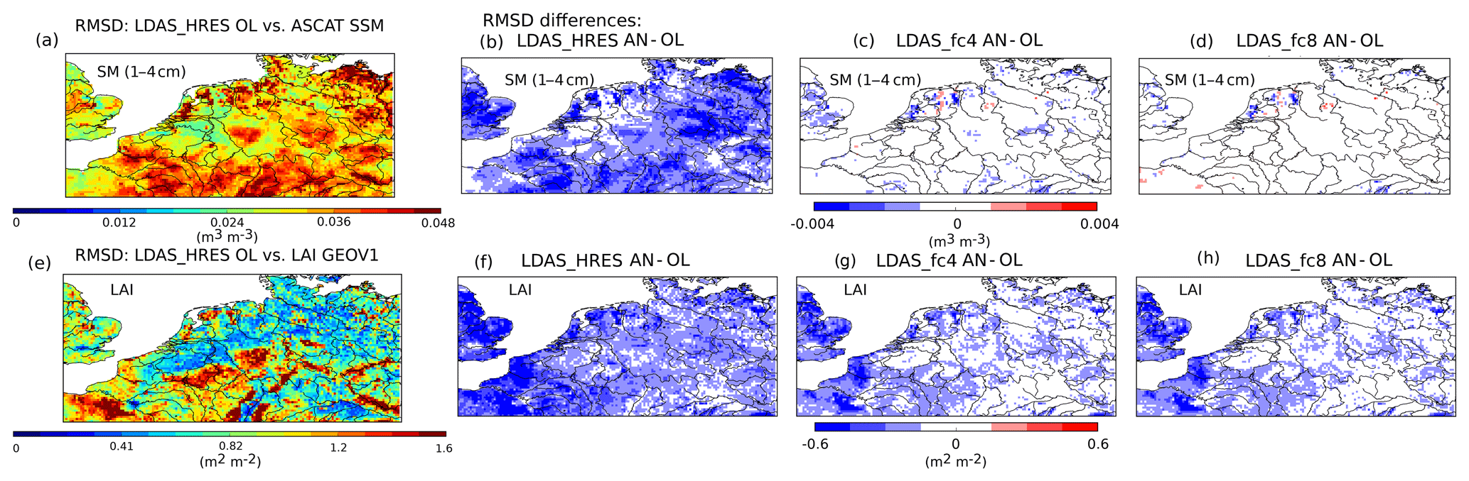
Figure 14 (a) RMSD values between LDAS_HRES open-loop and ASCAT SSM estimates over 2017–2018 for the WEUR domain; (b) RMSD differences between LDAS_HRES analysis (open-loop) and ASCAT SSM. (c), (d) and (e): same as (b) between LDAS_fc4 initialized by the analysis (open-loop) and LDAS_fc8. Bottom row: same as the top row for LAI from the different experiments and LAI GEOV1.

These results are corroborated by Figs. 14 (for WEUR) and 15 (for MUDA) for both SSM (top) and LAI (bottom). Figures 14a and 15a show RMSD values between LDAS_HRES open-loop SSM (1–4 cm) and ASCAT SSM over 2017–2018 for the WEUR and MUDA domains respectively. Due to the seasonal linear rescaling applied to ASCAT estimates, the RMSD values are rather small. For the WEUR (MUDA) domain they range from 0 to 0.048 m³ m⁻³ (0 to 0.040 m³m⁻³). Figures 14b and 15b present maps of RMSD differences between LDAS_HRES analysis (open-loop) and ASCAT SSM estimates over 2017–2018 for the WEUR and MUDA domains. Both maps are dominated by negative values (in blue) indicating that RMSD values are consistently smaller when using LDAS_HRES analysis than when using LDAS_HRES open-loop. For the MUDA domain, the RMSD values are reduced by about 15 %. Figures 14c, d and 15c, d show maps of RMSD differences for forecast experiments (LDAS_fc4, LDAS_fc8). It appears that over both domains, the impact from the initialization is rather small. This supports previous results indicating that the forcing quality is more important than the initial conditions for the SSM forecast. However, the results for LAI support the opposite conclusion. The RMSD values for LDAS_HRES open-loop range from 0 to 1.6 m² m⁻² over WEUR and 0 to 1 m² m⁻² over MUDA (Figs. 14e and 15e). The RMSD values are reduced by up to 37 % over WEUR and up to 60 % over MUDA by the analysis (Figs. 14f and 15f). The enhancement from the data assimilation is consistent throughout the WEUR domain, while the improvement over the MUDA domain is concentrated in the south-eastern part (the north-western part is largely unchanged).

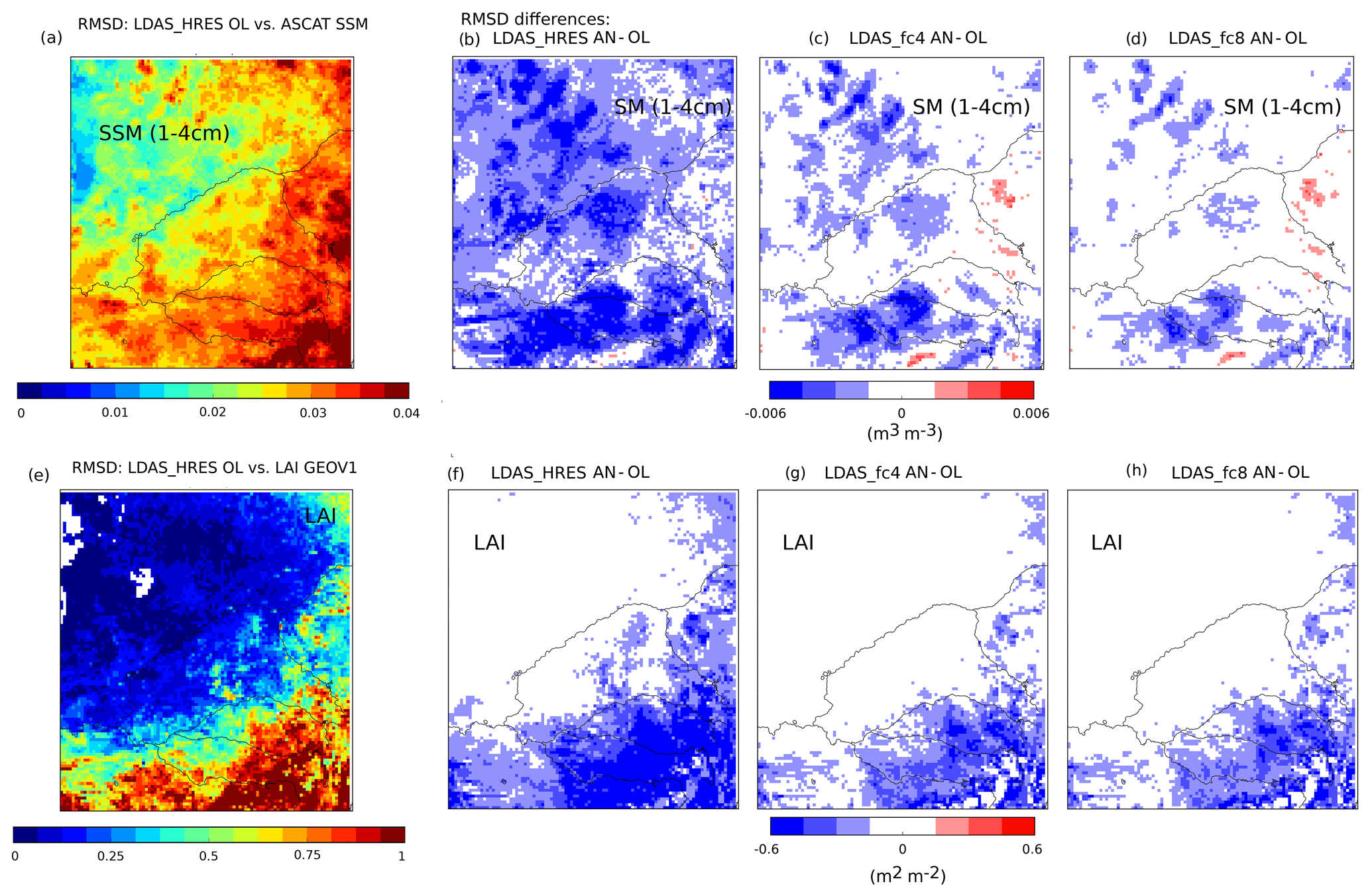
Figure 15 Same as Fig. 14 for the Murray–Darling River (MUDA) area in south-eastern Australia.

Similarly to Fig. 14a, b, c, d, Fig. 16 illustrates the impact of the analysis on SSM in terms of the correlation coefficient. But this time, ASCAT SWI (i.e. no rescaling) has been used for the validation. Figure 16 (top panels) shows maps of R values based on the absolute values, while Fig. 16 (bottom panels) shows R values based on the anomaly time series (capturing short-term variability) as defined in Albergel et al. (2018a). Figure 16a and e represent R values and anomaly R values for LDAS_HRES respectively. As expected, R values are higher than anomaly R values. Maps of differences (panels b and f) of Fig. 16 suggest that after assimilation, both scores are improved almost equally. The 4 and 8 d forecasts still show improvements from using initial conditions from the analysis over the open-loop on R values (Fig. 16c, d). Looking at R_anomaly values (Fig. 16g, h), no negative or positive impact from the initial conditions can be seen.

Finally, the top panels of Fig. 17 illustrate the impact of the analysis on drainage monitoring and forecasts over WEUR. Figure 17a represents drainage from the LDAS_HRES open-loop, with values ranging between 0 and 1 kg m⁻² d⁻¹. Figure 17b shows the drainage difference between LDAS_HRES analysis and open-loop. The analysis impact on drainage is rather small (within ±3 %) and more pronounced in areas where the analysis has largely affected LAI (see Fig. 14f, g and h). As seen in Fig. 17c and d, the forecasts are also sensitive to the initialisation in areas where the analysis effectively corrected LAI. The bottom panels of Fig. 17 illustrate a similar impact on runoff. Although we did not validate drainage and runoff in this study, previous findings suggest a neutral to positive impact of the analysis on river discharge through modifications to drainage and runoff (Albergel et al., 2017, 2018a).

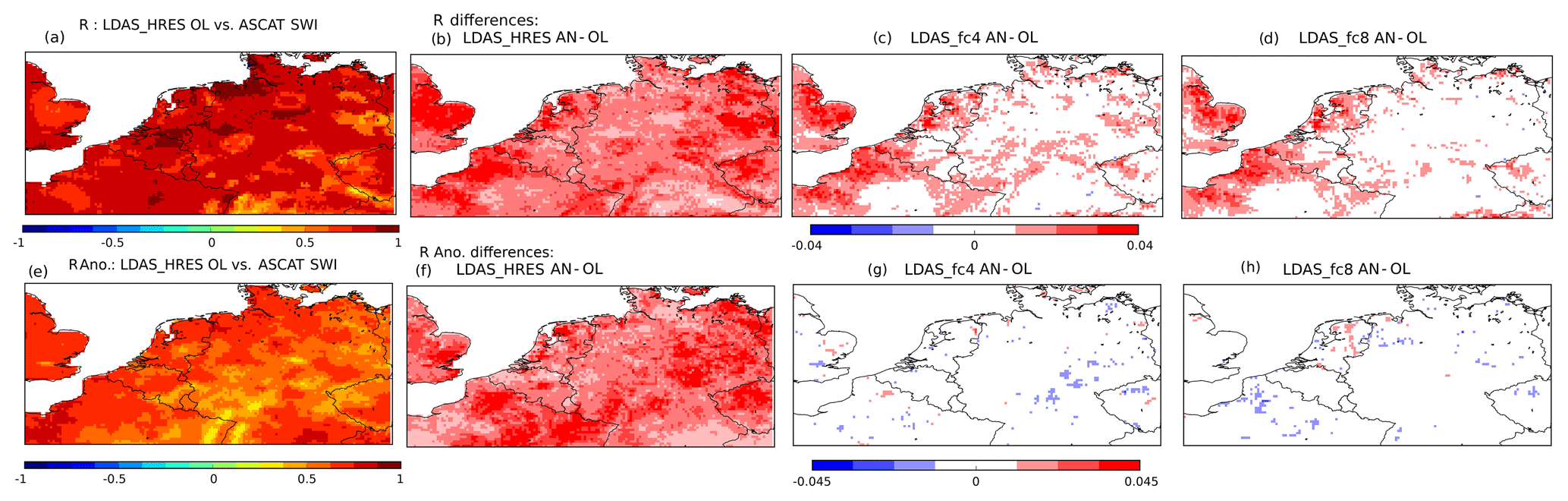
Figure 16 (a) R values between LDAS_HRES open-loop and ASCAT SWI estimates over 2017–2018 for the WEUR domain; (b) R differences between LDAS_HRES analysis (open-loop) and ASCAT SWI. (c) and (d): same as (b) between LDAS_fc4 initialized by the analysis (open-loop) and LDAS_fc8. Bottom row: same as top row for R values based on anomaly time series.

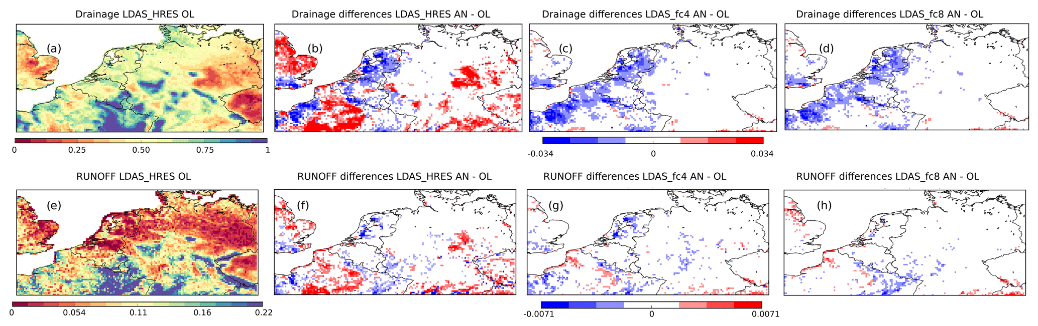
Figure 17 (a) Drainage values for LDAS_HRES open-loop over 2017–2018 for the WEUR domain; (b) drainage differences between LDAS_HRES analysis and open-loop. (c) and (d): same as (b) between LDAS_fc4 initialized by the analysis and LDAS_fc4 initialized by the open-loop and between LDAS_fc8 initialized by the analysis and LDAS_fc8 initialized by the open-loop. Bottom row: same as the top row for runoff. Units are kg m⁻² d⁻¹.

5 Discussion and conclusions

This study has demonstrated the potential of LDAS-Monde to assimilate Earth observations (EOs) into a land surface model (LSM) to predict the impact of heatwaves and droughts on land surface conditions. LDAS-Monde is now ready for various applications, including (i) land surface reanalyses of essential climate variables (ECVs), (ii) monitoring of water resources, such as the impact of droughts on vegetation, (iii) the detection of extreme land surface conditions; and (iv) the effective initialization of LSVs for land surface forecasting. LDAS-Monde has been applied in this study to past events of 2018 with respect to a relatively short climatology (2010–2018). It is planned that it will be applied to much longer periods for future reanalysis applications. The operational application of LDAS-Monde near-real time could potentially improve emergency monitoring systems for LSVs. Using high-quality atmospheric reanalyses like ERA5 to force LDAS-Monde guarantees a high level of consistency since the configuration is frozen in time (no changes in spatial and vertical resolutions, data assimilation or parameterizations). The coarse spatial resolution of ERA5 makes it affordable to run long time periods and large-scale LDAS-Monde experiments. With ERA5 available from 1979 and now covering near-real-time needs with its ERA5T version (https://climate.copernicus.eu/climate-reanalysis, last access: August 2020), an LDAS_ERA5 configuration would be able to provide a long-term climatology as well as near-real-time anomaly detections of the land surface conditions at coarse resolution (0.25^∘). Significant anomalies could then be used to trigger more focused “on-demand” simulations for regions experiencing extreme conditions. For these simulations, LDAS-Monde could be run at higher resolution by forcing the LSM with an enhanced resolution forecast in order to provide more information, such as the ECMWF operational high-resolution product (0.10^∘). The capability of such an approach was illustrated in our study for two regions in north-western Europe and south-eastern Australia. In terms of the RMSD, our results showed a very small impact of initial conditions on the forecasts of SSM. This was expected due to the short-term memory of the surface soil layer, which is dominated by the antecedent meteorological forcing. However, the LAI initialization had significant impact on the LAI forecast skill. This was also expected due to the long-term memory of vegetation evolution. For SSM, the assimilation is performed after a rescaling of the observations to the model climatology (see Sect. 2.3), which ensures that the model and observations are unbiased with respect to each other. However, LAI is not bias-corrected, which allows the assimilation process to remove bias in the modelled LAI (with respect to the observation). This technical difference between SSM and LAI assimilation, combined with the longer memory of LAI compared to SSM, contributes to the results presented in this study. Despite the expected behaviour of these two LSVs in forecasting, our results show that the LDAS-Monde system is capable of propagating the initial LAI conditions, which is relevant for LSV medium-range forecasting and potentially for longer lead times, such as seasonal forecasts. The strong impact of LAI initialization on the forecast does not seem to propagate to the surface soil moisture, and further studies are necessary to test the impact of initial conditions on other variables from LDAS-Monde (including soil moisture in deeper layers and evapotranspiration). Another possibility would be to force LDAS-Monde using the 51-member ECMWF ensemble forecasts. Although the ensemble system has coarser spatial resolution (∼0.20^∘) than the deterministic forecast, it accounts for forcing uncertainty in the LSVs through the ensemble spread and extends to a 15 d lead time. The maximum range of the soil and vegetation forecasts could even be extended to 6 months if seasonal atmospheric forecasts were used as forcing.

LDAS-Monde has some limitations, where future developments are needed to improve the representation of LSVs. For instance, it does not consider snow data assimilation yet. It has been shown in this study that if the snow accumulation seems to be represented correctly in the system, the onset of snowmelt is too early in the spring. To overcome this issue, two possibilities will be explored. Firstly, a recently developed ISBA parametrization, MEB (Multiple Energy Budget), is known to lead to a better representation of the snowpack (Boone et al., 2017). This could be particularly useful in the densely forested areas of the Northern Hemisphere, where large differences between LDAS-Monde and the IMS snow cover were found in spring (Fig. S2i, Aaron Boone CNRM, personal communication, June 2019). Another enhancement of LDAS-Monde will be to adapt the current data assimilation scheme to permit the assimilation the IMS snow-cover data, which is implemented at NWP centres such as the ECMWF (de Rosnay et al., 2014). The current SEKF data assimilation scheme is also being revisited. Even though it has provided good results, one of its limitations is the computational cost of the Jacobian matrix, which needs one model run for each control variable. As the number of control variables is expected to increase, this approach would require significant computational resources. Therefore, more flexible ensemble-based data assimilation approaches have recently been implemented in LDAS-Monde, such as the ensemble square root filter (EnSRF, Fairbain et al., 2015; Bonan et al., 2020). Bonan et al. (2020) have evaluated performances from the EnSRF and the SEKF over the Euro-Mediterranean area. Both data assimilation schemes have a similar behaviour for LAI while for SSM, the EnSRF estimates tend to be closer to observations than those from the SEKF. They have also conducted an independent evaluation of both assimilation approaches using satellite estimates of evapotranspiration and GPP together with river discharge observations from gauging stations. They have found that the EnSRF gives a systematic (moderate) improvement for evapotranspiration and GPP and a highly positive impact on river discharges, while the SEKF leads to more contrasting performance. As for applications in hydrology, the 0.5^∘ spatial resolution TRIP river network is currently being improved to 1∕12^∘ globally.

CNRM is also investigating the direct assimilation of ASCAT radar backscatter (Shamambo et al., 2019). This has the potential to improve the way vegetation is accounted for in the change detection approach used to retrieve SSM with an improved representation of its effect. Assimilating ASCAT radar backscatter also raises the question of how to properly specify SSM observation, background, and model error covariance matrices, which are currently based on soil properties (see Sect. 2.1.3 on data assimilation). The last decade has seen the development of techniques to estimate those matrices. Approaches based on Desroziers diagnostics (Desroziers et al., 2005) are computationally affordable for land data assimilation systems and could provide insightful information on the various sources of the data assimilation system.

Furthermore, a comparison of LDAS-Monde with existing datasets from other centres needs to be considered. Current work at Météo-France has began to compare its quality against state-of-the-art reanalyses such as those from NASA at both the global scale (GLDAS, Rodell et al., 2004, MERRA-2, Reichle et al., 2017; Draper et al., 2018) and regional scale (NCALDAS over the continental USA, FLDAS over Africa). Finally, first work has begun to run LDAS-Monde at kilometric- and sub-kilometric-scale spatial resolutions. Promising results have been obtained by assimilating SSM and LAI over the AROME domain (Applications de la Recherche à l'Opérationnel à Méso-Echelle, https://www.umr-cnrm.fr/spip.php?article120, last access: July 2019) of Météo-France.