the Creative Commons Attribution 4.0 License.
the Creative Commons Attribution 4.0 License.
 | 20 Aug 2020
Evaluation of the WMO Solid Precipitation Intercomparison Experiment (SPICE) transfer functions for adjusting the wind bias in solid precipitation measurements
Amber Ross
John Kochendorfer
Michael E. Earle
Mareile Wolff
Samuel Buisán
Yves-Alain Roulet
Timo Laine
The World Meteorological Organization (WMO) Solid Precipitation Intercomparison Experiment (SPICE) involved extensive field intercomparisons of automated instruments for measuring snow during the 2013/2014 and 2014/2015 winter seasons. A key outcome of SPICE was the development of transfer functions for the wind bias adjustment of solid precipitation measurements using various precipitation gauge and wind shield configurations. Due to the short intercomparison period, the data set was not sufficiently large to develop and evaluate transfer functions using independent precipitation measurements, although on average the adjustments were effective at reducing the bias in unshielded gauges from −33.4 % to 1.1 %. The present analysis uses data collected at eight SPICE sites over the 2015/2016 and 2016/2017 winter periods, comparing 30 min adjusted and unadjusted measurements from Geonor T-200B3 and OTT Pluvio2 precipitation gauges in different shield configurations to the WMO Double Fence Automated Reference (DFAR) for the evaluation of the transfer function. Performance is assessed in terms of relative total catch (RTC), root mean square error (RMSE), Pearson correlation (r), and percentage of events (PEs) within 0.1 mm of the DFAR. Metrics are reported for combined precipitation types and for snow only. The evaluation shows that the performance varies substantially by site. Adjusted RTC varies from 54 % to 123 %, RMSE from 0.07 to 0.38 mm, r from 0.28 to 0.94, and PEs from 37 % to 84 %, depending on precipitation phase, site, and gauge configuration (gauge and wind screen type). Generally, windier sites, such as Haukeliseter (Norway) and Bratt's Lake (Canada), exhibit a net under-adjustment (RTC of 54 % to 83 %), while the less windy sites, such as Sodankylä (Finland) and Caribou Creek (Canada), exhibit a net over-adjustment (RTC of 102 % to 123 %). Although the application of transfer functions is necessary to mitigate wind bias in solid precipitation measurements, especially at windy sites and for unshielded gauges, the variability in the performance metrics among sites suggests that the functions be applied with caution.
- Article
(3015 KB) - Full-text XML
- BibTeX
- EndNote


The World Meteorological Organization (WMO) Solid Precipitation Intercomparison Experiment (SPICE) was a Commission for Instruments and Methods of Observation (CIMO) initiative to assess and compare instruments and methods for measuring solid precipitation (Nitu et al., 2012, 2018). The objectives were (1) to make recommendations for appropriate automated field reference systems and (2) to provide guidance on the performance and operation of automated systems for measuring solid precipitation and snow on the ground. SPICE was motivated by the need for accurate and homogenized solid precipitation measurements. For example, such measurements are required for climate trend analysis in northern regions (e.g. Førland and Hanssen-Bauer, 2000; Yang and Ohata, 2001, Scaff et al., 2015). Following historical works on adjusting the systematic undercatch of solid precipitation measurements due to wind (Goodison, 1978; Sevruk et al., 1991, 2009; Goodison et al., 1998; Smith, 2009; Wolff et al., 2015; Kochendorfer et al., 2017a; Buisán et al., 2017), a methodology and a set of widely applicable transfer functions for the adjustment of high-resolution (i.e. 30 min) precipitation measurements was developed. The SPICE transfer functions discussed in this study were developed for single Alter-shielded or unshielded automated precipitation gauges (Kochendorfer et al., 2017b). Because of the symbioses between the Kochendorfer et al. (2017b) SPICE work and this evaluation, the SPICE methodology is described below in more detail and henceforth referred to as K2017b.
The official SPICE intercomparison period occurred during the winters of 2013/2014 and 2014/2015. During this period, a Double Fence Automated Reference (DFAR) was operated at the following eight test bed sites: Bratt's Lake (XBK), Caribou Creek (CCR), the Centre for Atmospheric Research and Experiments (CARE; shortened to CAR), Formigal (FOR), Haukeliseter (HKL), Marshall (MAR), Sodankylä (SOD), and Weissfluhjoch (WFJ; Fig. 1; Table 1). The DFAR was developed for use as the field reference configuration for SPICE (Nitu, 2012; Nitu et al., 2016, 2018). Descriptions of each site, complete with detailed layouts and photos, are available in the WMO-SPICE site commissioning reports (http://www.wmo.int/pages/prog/www/IMOP/intercomparisons/SPICE/SPICE.html, last access: 12 August 2020) and in the WMO-SPICE final report (IOM Report no. 131 found at http://www.wmo.int/pages/prog/www/IMOP/publications-IOM-series.html, last access: 12 August 2020; Nitu et al., 2018).
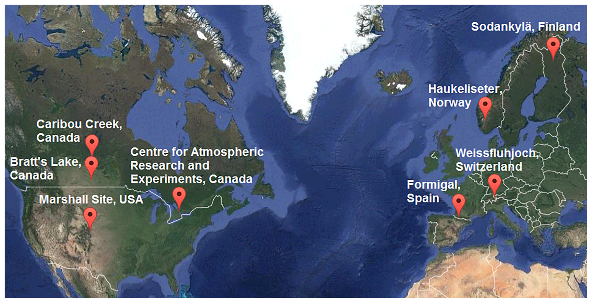
Figure 1The SPICE intercomparison sites used in the development and evaluation of the SPICE transfer functions. (Source: base map obtained from Google Earth; data – Scripps Institution of Oceanography (SIO), US Navy, and the General Bathymetric Chart of the Oceans (GEBCO); © 2018 Google; image – Landsat/Copernicus.)
Table 1Site name (and country), abbreviation, latitude, elevation above sea level, mean daily air temperature, and relative total amounts of precipitation by phase (snow, mixed, or rain).
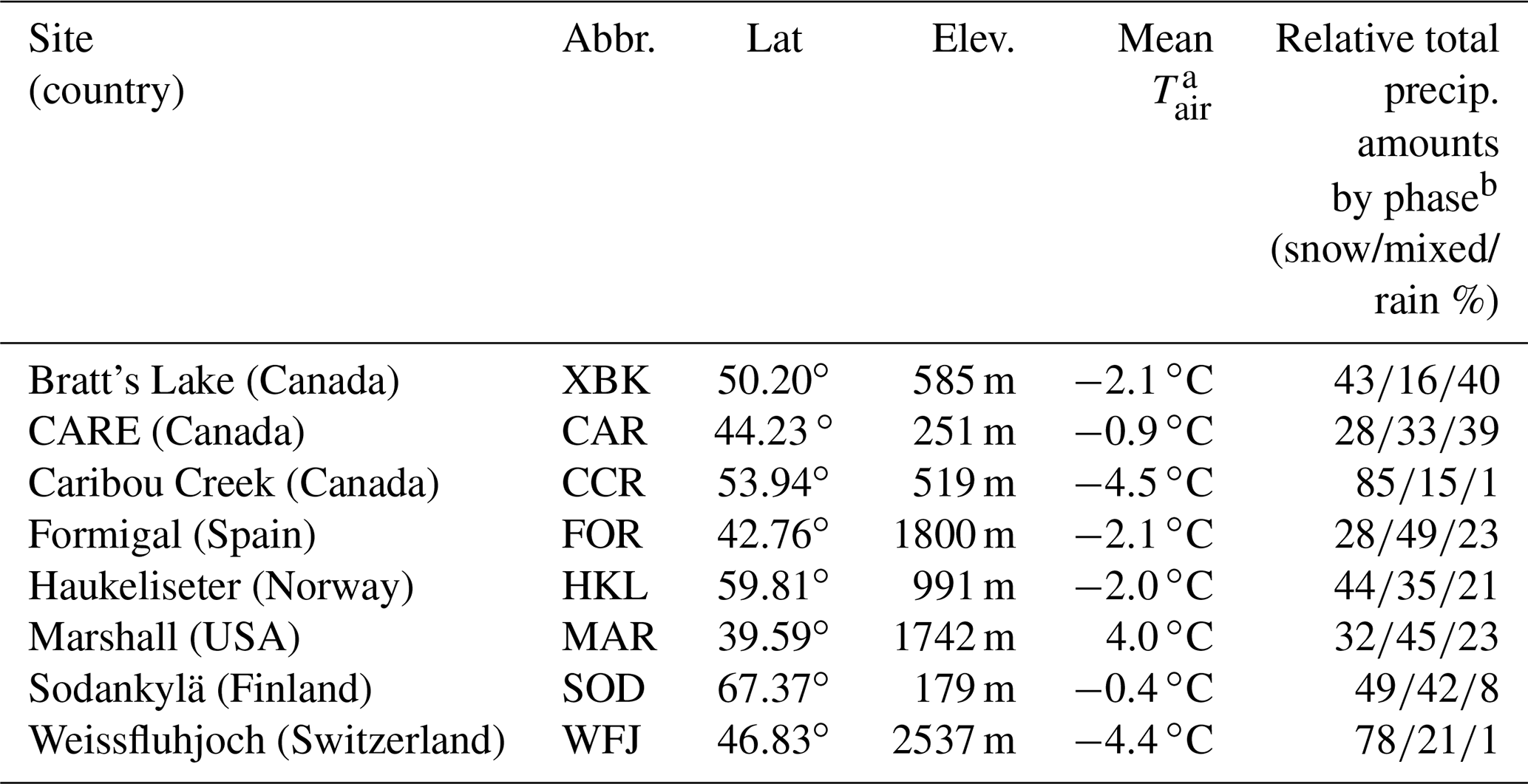
a Daily average mean air temperature over the year from site climatology (Nitu et al., 2018). b As measured by the DFAR for the October–April periods of 2015/2016 and 2016/2017 and calculated using the temperature thresholds listed in Sect. 1.1.
The DFAR consisted of either a Geonor T-200B3 or an OTT Pluvio2 automated weighing precipitation gauge with a single Alter-shield inside the same large octagonal double fence used for the WMO's Double Fence Intercomparison Reference (DFIR). The DFIR was employed as a manual field reference configuration during previous solid precipitation intercomparisons (Yang et al., 1993; Goodison et al., 1998). The DFAR incorporated a precipitation detector to reduce the probability of including false precipitation reports in SPICE data analysis. The result was the development of a high-confidence reference precipitation data set called the site event data set (SEDS; Reverdin, 2016). In the SEDS, a precipitation event was a 30 min period during which a precipitation detector (typically an optical disdrometer capable of identifying the occurrence of even light precipitation) observed precipitation for at least 18 min during the 30 min period (60 % of event duration), and the DFAR measured ≥0.25 mm. The justification for the filtering criteria used in K2017b is detailed in Kochendorfer et al. (2017a). The SEDS was then used to produce the SPICE transfer functions. By combining data from each site in Table 1, the intent was to make these multisite transfer functions universally applicable.
1.1 The K2017b transfer functions
The transfer functions presented in K2017b were developed for both unshielded and single Alter-shielded automated precipitation gauges by combining observations from the Geonor T-200B3 and OTT Pluvio2 gauges (hereafter referred to as the sensors under test, or SUT), after the authors demonstrated that the unshielded catch from both SUT types were very similar. Using the SEDS, further processing was applied to the SUT data (as justified in Kochendorfer et al., 2017a) using a minimum 30 min threshold defined as the median of the ratio of the SUT accumulation to that of the DFAR for the precipitation event threshold of 0.25 mm. This prevented the results from becoming biased towards the gauge used in the SEDS event selection. For wind speed, K2017b used the wind speed measurements available at each site and applied the log profile law to produce a 30 min average wind speed for both the gauge height (Ugh) and the standard 10 m height (U10 m), either increasing speeds to U10 m or decreasing speeds to Ugh, depending on which measured wind height speed data was deemed the best at each site. Catch efficiencies (CE) were then calculated for each event as the ratio of the 30 min SUT precipitation accumulation to that of the DFAR over the same period. From K2017b, two functional forms were used to fit the data as follows:
and
where U is wind speed (specifically either Ugh or U10 m) in m s−1, Tair is air temperature in ∘C, and a, b, and c are coefficients to fit the data to the model. Equations (1) and (2) listed here are referred to as Eqs. (3) and (4) in K2017b. To reduce the impact of fewer events at higher wind speeds and the potential impacts of blowing snow, the SEDS data were filtered further to remove events with wind speeds higher than 7.2 m s−1 (9 m s−1) at the gauge height (10 m).
The key difference between Eqs. (1) and (2) is the inclusion of temperature dependency in Eq. (1). This allows for a continuous (3D) transfer function at all temperatures without having explicit knowledge of the precipitation phase. This curve is shown in Fig. 2 (red) for both the single Alter-shielded (solid) and unshielded (dashed) gauges at a temperature of −5 ∘C. Equation (2), however, requires an assessment of the precipitation phase (liquid, solid, or mixed), with each phase having unique coefficients. K2017b used temperature to discriminate the phases for Eq. (2) and assumed the following: solid precipitation occurs at ∘C, liquid precipitation occurs at Tair>2 ∘C, and mixed precipitation occurs at −2 ∘C ≤ Tair ≤ 2 ∘C. The temperature thresholds for phase discrimination in the SPICE analysis are based on the disdrometer measurements of precipitation type from Wolff et al. (2015) and Kochendorfer et al. (2017a). Equation (2) is plotted in Fig. 2 (blue) using the coefficients for snow for the single Alter-shielded (solid) and unshielded (dashed) gauges. For both equations and gauge configurations, unique coefficients were derived for each of the two wind speed measurement heights. The SUT precipitation was adjusted using both Eqs. (1) and (2) by employing the appropriate coefficients, depending on the phase and/or temperature, wind measurement height, and shield configuration. For Eq. (2), precipitation classified as rain (Tair>2 ∘C) was assumed a CE equal to 1. The coefficients used in Eqs. (1) and (2) are detailed in K2017b and are not repeated here. Kochendorfer et al. (2017a, b) examined the use of more complex transfer function forms for adjusting solid precipitation measurements, such as the sigmoid function used by Wolff et al. (2015), but found that the simpler forms had similar bias and RMSE characteristics as the more complex forms.

Figure 2WMO-SPICE transfer functions from K2017b, Eq. (1; red), Eq. (2; blue) for unshielded (dashed), and single Alter-shielded (solid) gauges. Equation (1) is plotted using an air temperature of −5 ∘C, and Eq. (2) is plotted for snow. Both transfer functions are plotted for Ugh, with the maximum wind speed threshold shown at 7.2 m s−1.
1.2 K2017b results
Following the end of the SPICE project, the performance of the SPICE transfer functions was evaluated as described in K2017b, using the same SEDS data used to develop those transfer functions. As discussed above, the data from all eight sites in Table 1, including data from multiple gauges of the same configuration at each of the sites, were combined to fit the transfer function models. This model, developed by pooling the data from multiple sites, was then applied to each individual gauge at each site. By applying a model developed from data collected at multiple sites to individual gauges at each individual site, the authors maintained some distinction between the model development and the evaluation. The K2017b results were based on four metrics, namely the root mean square error (RMSE), mean bias, Pearson correlation (r), and percentage of events (PEs) between the DFAR and SUT that agreed within a specified threshold (typically 0.1 mm). It should also be noted that the overall performance metrics summarized in K2017b included all precipitation phases, whether adjusted by the transfer functions (i.e. solid and mixed) or not (i.e. liquid).
K2017b showed that the SPICE transfer functions reduced the overall bias in the unshielded precipitation gauges (both Geonor T-200B3 and OTT Pluvio2; all sites combined) from −33.4 % to 1.1 %, but the results varied by site, with CAR and WFJ showing an over-adjustment and HKL, FOR, and XBK showing an under-adjustment. For the most part, the r, RMSE, and PEs were slightly improved after the adjustment, but these also varied by site. K2017b also showed that, in general, the mountainous sites experienced larger errors after the adjustment, with one mountainous site (WFJ) being over-adjusted and the other two (HKL and FOR) being under-adjusted.
1.3 Motivation for the extended evaluation
The impetus for this extended evaluation was twofold:
-
The methodology used during SPICE for developing and evaluating the transfer functions used only a subset of the observed data (the SEDS), and although this was a robust methodology for developing transfer functions, it did not provide a comprehensive evaluation of the adjustments under circumstances more typical of users collecting precipitation data in the field where the data are less filtered to remove smaller amounts.
-
The data set used for the evaluation of transfer functions in K2017b was not completely independent of that used to develop the functions. A robust assessment requires additional data collected following the end of the SPICE intercomparison period that was not used in the development of the transfer functions.
This evaluation will examine the performance of the SPICE transfer functions for precipitation measurements from each of the eight intercomparison sites shown in Fig. 1 for the 2015/2016 and 2016/2017 winter seasons. Each of these sites continues to operate a DFAR following the SPICE intercomparison period, which is a critical component for assessing transfer function performance. The assessment will be conducted for both unshielded and single Alter-shielded gauges using wind speed heights of 10 m and gauge height, where available. Extending the K2017b evaluation, this assessment will consider transfer function performance using both (1) data over the entire winter season, regardless of precipitation phase, and (2) solid precipitation measurements only, to focus on the most challenging and critical adjustments.
Precipitation and ancillary meteorology data at a 1 min resolution for the 2015/2016 and 2016/2017 winter periods were obtained from the eight SPICE sites. The data were quality controlled using the same techniques employed in SPICE (Nitu et al., 2018), which involved automated range and jump checks and supervised removal of remaining outliers. Where available, service logs were provided by site hosts to assist in data quality control and the identification of outliers due to servicing (e.g. rapid drops or increases in precipitation gauge bucket weights) or maintenance (e.g. instrument malfunctions or other human interventions that may impact the data). The Geonor T-200B3 gauges employed three transducers, and the output from all three were averaged to produce a single time series. Next, the high-resolution precipitation data were subjected to the same Gaussian filter as the SPICE data used in K2017b to dampen high-frequency noise; however, it was decided to not develop an event database, such as the SEDS, but rather to use an alternate process to develop a consistent 30 min precipitation time series to more closely reflect real-world precipitation data sets. This alternate process involves the use of a modified “brute force” filter, initially described in Pan et al. (2016), henceforth called the neutral aggregation filter (NAF). NAF is described in more detail in Smith et al. (2019a).
2.1 Neutral aggregation filter
The NAF algorithm removes noise in cumulative precipitation time series by iteratively balancing positive and negative noise and accumulating positive changes exceeding the noise by a user-defined threshold (Δ*; e.g. 0.05 or 0.2 mm, depending on the gauge precision; Smith et al., 2019a) such that the total accumulated positive increases in bucket weight after filtering are forced to equal the total end-of-season bucket weight. The algorithm removes random and systematic diurnal noise but does not account for signal drift (an example of signal drift is a decrease in weight that occurs due to evaporation of water from the gauge bucket). Signal drift can result in estimation errors, which can be mitigated using an iterative manual process, with the NAF output as a first guess. This process is called NAF supervised (NAF-S) and lets the user select the beginning and the end points of the segments within the time series where evaporation is occurring. The process then removes these segments so that they have no impact on the time series. Because there is some user subjectivity in selecting the beginning and end points of the impacted segments, this process is completed by a single user employing predetermined and consistent criteria. Although beyond the scope of the present work, testing NAF and NAF-S on both simulated and observed precipitation time series over an entire winter season, including both noise and evaporation drift, showed the technique to be effective, with low error compared to the control. The end product of the NAF-S filter is a clean, time-consistent 1 min accumulating time series with preserved data gaps (i.e. no gap filling) for each gauge configuration for each season.
2.2 Amalgamation and adjustment
To produce accumulation periods consistent with the K2017b validation, the 1 min NAF-S precipitation accumulation time series were resampled to 30 min accumulation amounts via differentiating the bucket weights between the start and end of the 30 min period. The continuity of the time series was maintained, despite data gaps, through the assumption that the gauge continues to accumulate precipitation despite logger or power outages. In the event of missing data, precipitation accumulation during outages was calculated based on the differential bucket weight between the start and end of the outage and recorded as an accumulation at the end of the outage. Although this preserves the total accumulation during the outage, information related to the timing of the events during the outage is not preserved, and the accumulation data need to be flagged. Protocols for adjusting the data for undercatch are noted below.
The 1 min wind speeds (U10 m and Ugh, where available) and air temperatures (generally measured at 1.5 m) were averaged over the same 30 min periods as the accumulated precipitation amounts. Site-specific details on the ancillary measurements can be found in the SPICE site commissioning reports (referenced in Sect. 1). If more than 10 min of wind or temperature data were missing in any 30 min period, the data were flagged as missing and were not used in the adjustment procedure.
The resultant time series for each test gauge at each site were adjusted separately using both Eqs. (1) and (2). Each 30 min accumulation was adjusted individually if the following conditions were met: (1) both the start and end bucket weights for the 30 min period were not missing, such that the differential could be determined, and (2) no more than 10 of the 30 min values of either wind speed or temperature were missing. Periods that did not meet these criteria were preserved in the time series but were flagged as being unadjusted and were not included in the validation.
For adjustments using Eq. (1), the predetermination of the precipitation phase was not necessary as the transfer function is continuous with temperature and not directly dependent on the precipitation phase. For the purpose of adjusting precipitation using Eq. (2), the phase is determined by air temperature using the phase regimes outlined in Sect. 1.1 with rain assuming a catch efficiency of 1 (and is therefore not adjusted). The relative total amounts (snow, mixed, and rain), as measured by the DFAR at each site, are shown in Table 1. The same maximum wind speed thresholds for the adjustments were employed here as in K2017b, which were 7.2 and 9.0 m s−1 at gauge height (generally 2 m above ground) and at a 10 m height, respectively. Wind speeds above these thresholds were set at the threshold value to avoid over-adjustment and increased uncertainty in the transfer functions above the wind speed threshold. Figure 2 suggests that Eq. (2) can exceed a catch efficiency of 1 at low wind speeds. There is no obvious physical explanation for the portion of the Eq. (2) catch efficiency function (originally published by K2017b) that is >1.0, and this is related to the empirical fit of the catch efficiency curve to the original SPICE data. For the current assessment, calculated catch efficiencies > 1 were infrequent, and occurrences were automatically set to 1.
The resulting data (https://doi.org/10.1594/PANGAEA.907379; Smith et al., 2019b) include a subset of adjusted and unadjusted 30 min precipitation amounts for each SUT gauge configuration at each site (adjusted using Eqs. (1) and (2), using either Ugh or U10 m or both, where available), the 30 min DFAR data, and the accumulated gap-preserved time series for each, with flags identifying the periods that were not adjusted.
2.3 Performance assessment
Four complementary statistical metrics are used to assess the performance of the transfer functions for adjusting precipitation. These are relative total catch (RTC), root mean square error (RMSE), Pearson correlation (r), and percentage of events (PEs) within 0.1 mm of the DFAR-reported values. RTC is the ratio of accumulated catch of the SUT to that of the reference over the same period and using the same filter or thresholds (i.e. for snow). RTC is expressed as a percentage of the reference precipitation amount and reflects the capability of the transfer functions to adjust seasonal and long-term precipitation totals, with a perfect seasonal adjustment having an RTC of 100 %. Hence, it can be used to assess the improvement in the seasonal bias following the adjustment.
Root mean square error is used to estimate the magnitude of uncertainty in the 30 min unadjusted and adjusted SUT measurements relative to the DFAR. The ideal value of the RMSE is 0 mm, indicating a perfect agreement between the 30 min SUT observations and those from the reference; however, the variability in the magnitude of the RMSE amongst the sites should be interpreted with caution as a small RMSE at a site with low precipitation rates may be more significant than a higher RMSE at a site that has higher precipitation rates. For that reason, the RMSE will be used mainly to assess the relative performance of Eqs. (1) and (2) at each site and the relative performance of the transfer functions for the single Alter-shielded and unshielded gauges.
The Pearson correlation assesses the strength of the linear correlation between the 30 min measurements made with the SUT and the reference DFAR before and after adjustments, using Eqs. (1) and (2). This metric provides an overall indication of the changes in the differences between SUT and reference measurements but does not provide an indication of the changes in the bias or the magnitude of differences.
The PE statistic is the percentage of 30 min events measured by the SUT that differs from the DFAR by less than a predefined threshold (0.1 mm in this analysis) and is calculated as follows:
where n is the number of 30 min events considered in the analysis and nT is the size of the subset of n where |DFAR − SUT mm. PE was introduced as a metric for assessing transfer functions in K2017b, with the 0.1 mm threshold based on the measurement uncertainty of the reference configuration as investigated during WMO-SPICE (Nitu et al, 2018). Ideally, applying a transfer function to adjust the systematic bias (undercatch) in precipitation measurements would increase the magnitude of SUT observations to be closer to the reference measurements, thereby increasing PEs. A perfect agreement between the reference and the SUT, within the 0.1 mm threshold, would produce a PE of 100 %. Hence, PE provides additional event-based perspectives on how adjustments impact the bias and uncertainty that are not captured by the other metrics used in the assessment.
The assessment considers the overall performance for all precipitation types combined and for snow alone. In the latter case, the assessment of snow adjustments using Eq. (1) employs the same temperature threshold for snow as K2017b, namely ∘C. Assessment results are reported for both unshielded and single Alter-shielded gauge configurations, which can be either a Geonor T-200B3 or OTT Pluvio2. Where multiple gauges of the same configuration are present at a site, these gauges are assessed both individually and as a combined data set.
For evaluation purposes, and where possible, the following circumstances are assessed for all precipitation types (including rain, snow, and mixed) and snow only: (a) adjustments using Eq. (1) vs. Eq. (2), (b) adjustments using gauge height vs. 10 m wind speeds, and (c) adjusting single Alter-shielded vs. unshielded gauges. Based on site-by-site evaluations, some insight is provided as to the performance of transfer functions in different environments and under different climate characteristic conditions.
3.1 Time series
The impact and the performance of transfer functions used for adjusting precipitation can be examined by comparing the accumulation time series for unadjusted and adjusted data to the reference. Figures 3 and 4 show the unadjusted, adjusted (Eq. (1) only), and reference (DFAR) time series of precipitation accumulation for the unshielded and single Alter-shielded gauges at all sites for the 2015/2016 and 2016/2017 winter seasons, respectively. Where more than one gauge with the same shield configuration was present at a site, and where more than one wind speed height was available, results for only one gauge and wind speed height were selected for illustrative purposes.
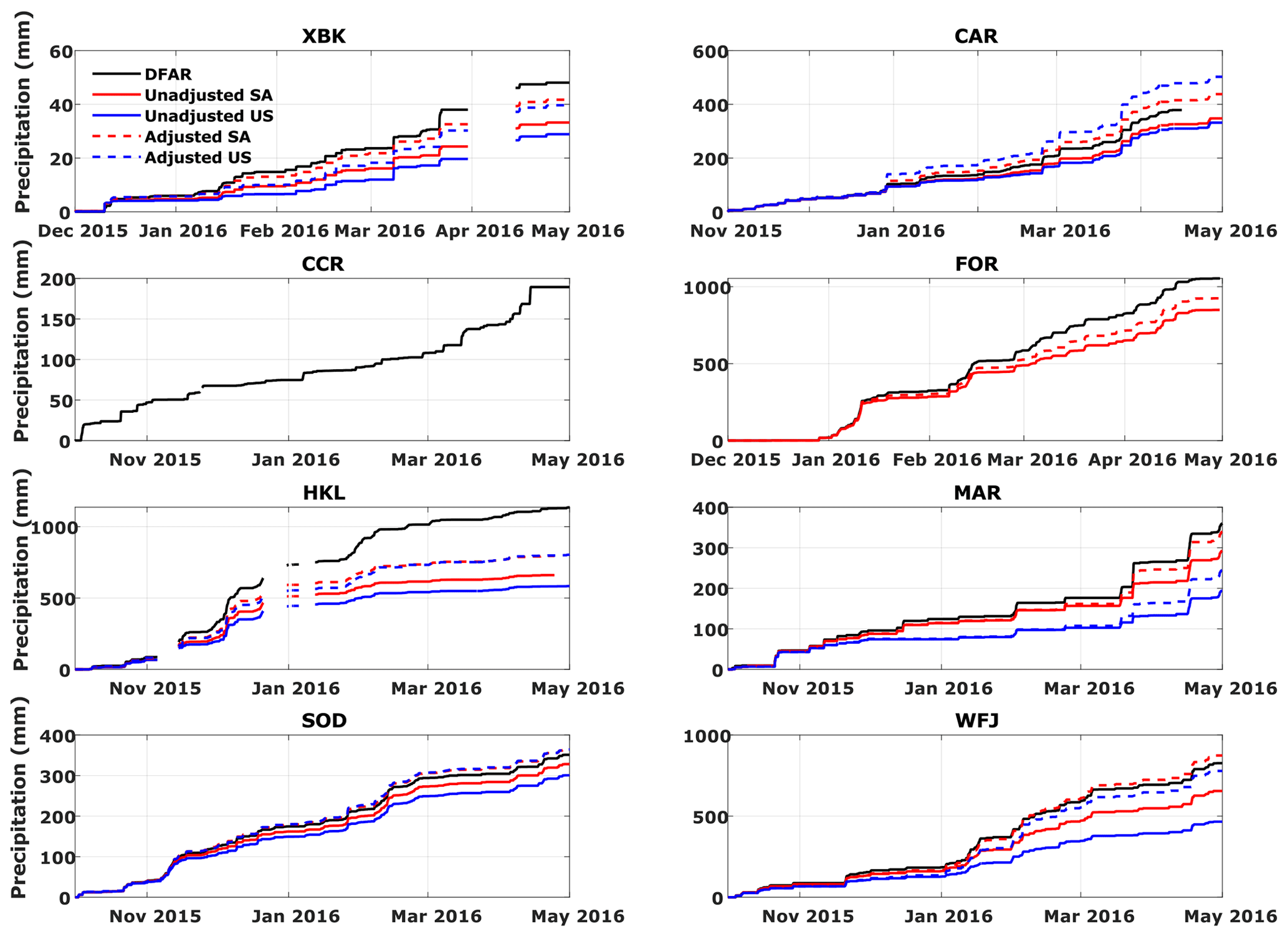
Figure 3Time series of unadjusted (solid) and adjusted (dashed) precipitation time series for single Alter-shielded (red) and unshielded (blue) gauges as compared to the DFAR (black) during the 2015/2016 winter season at the eight SPICE sites.

Figure 4Time series of unadjusted (solid) and adjusted (dashed) precipitation time series for single Alter-shielded (red) and unshielded (blue) gauges as compared to the DFAR (black) during the 2016/2017 winter season at the eight SPICE sites.
Figures 3 and 4 show the relative impacts of wind on undercatch for each of the eight sites and the relative effectiveness of the transfer function adjustments on each SUT configuration (shielded and unshielded) for the two winter seasons separately. Note that the season lengths vary by site and season (depending on both the actual length of the winter season and on data availability), and the scale of the vertical axis changes with site and season to show the relative scale of the bias and the adjustment. Gaps in the series represent missing data, with total accumulations during the gap obtained from the bucket weight change (in both the DFAR and the SUT); the gap accumulations were preserved but not adjusted.
The precipitation amounts vary by site and season, but the general trends in the SUT undercatch, compared to the DFAR, are consistent. Accordingly, the impact of the adjustment also appears to be consistent. Without considering precipitation-phase partitioning, unadjusted precipitation (solid lines) relative to the DFAR was always lowest at the windy sites of XBK and HKL. Referring to unadjusted precipitation, unshielded gauges (blue lines) always catch less precipitation than the single Alter-shielded gauges (red lines) at all sites and during both winters. The transfer function (only temperature-dependent Eq. (1) adjustments are shown here) appears to be less effective at the windier sites (wind speeds during precipitation events are shown in Table 2), with a substantial undercatch remaining after the adjustment. Furthermore, precipitation is over-adjusted at some of the less windy sites (CAR, CCR, and SOD).
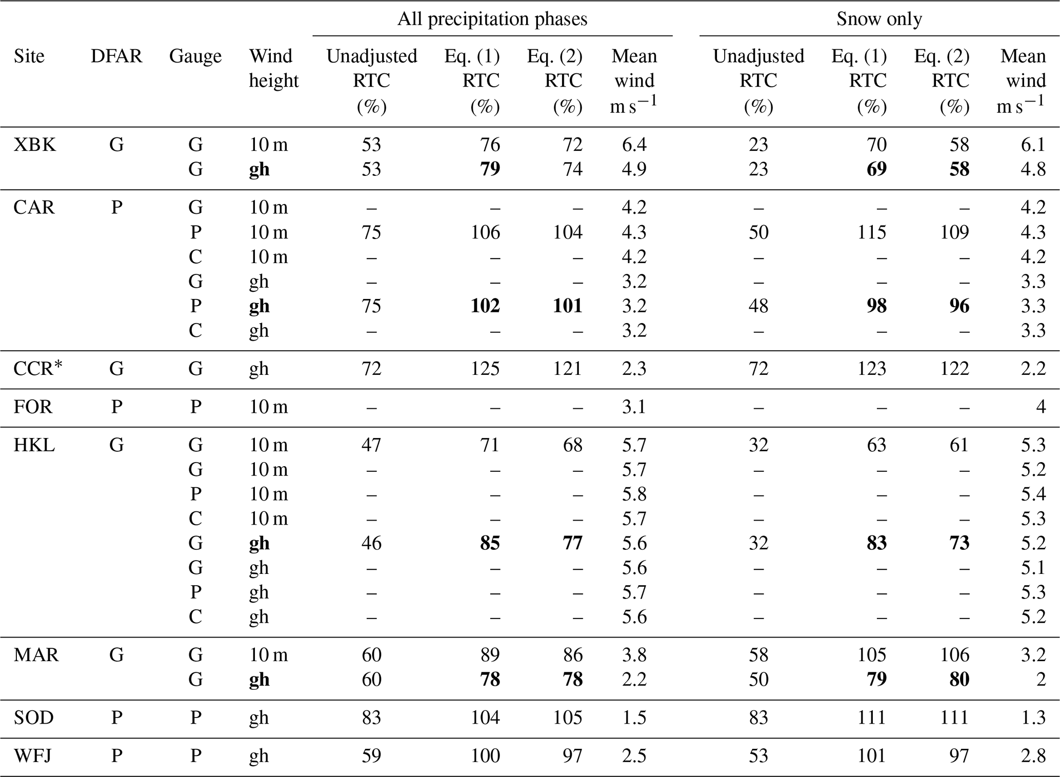
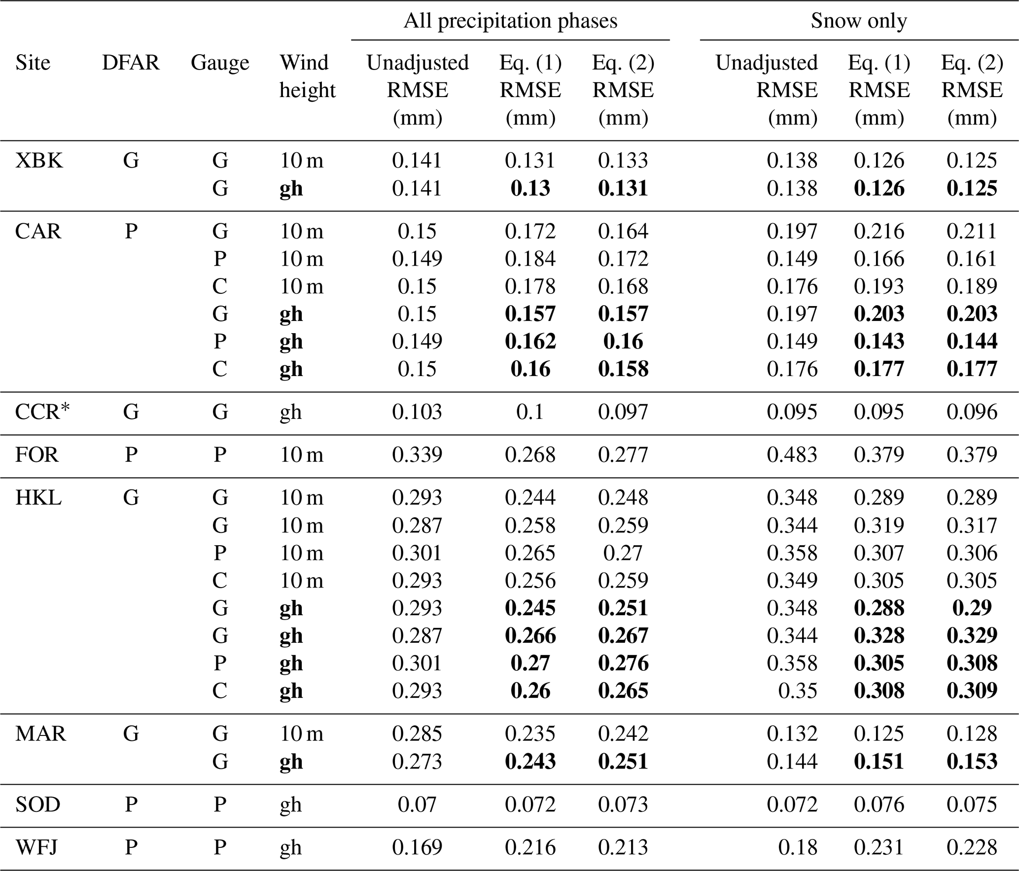
Table 2Relative total catch (RTC) for the single Alter-shielded gauges (G – Geonor; P – Pluvio2) as compared to the DFAR reference at each site for the combined winters of 2015/2016 and 2016/2017. Results are provided for available wind speed measurement heights (10 m; gh – gauge height) and for Eqs. (1) and (2). Metrics are separated by precipitation phase (all and snow only). Where both wind speed heights are available, the gauge height data are shown in bold.
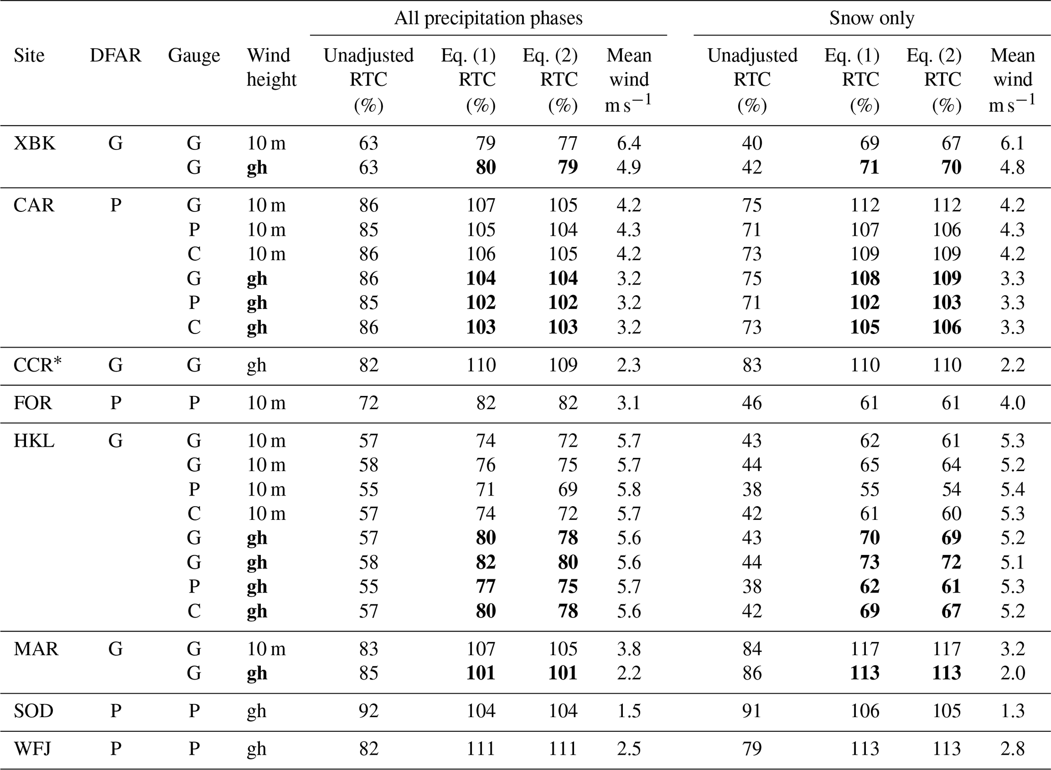
* Indicates 2016/2017 winter only.
3.2 Relative total catch
The RTC metrics for the single Alter-shielded gauges are shown in Table 2 and for the unshielded gauges in Table 3 for Eqs. (1) and (2), combining the data from the two intercomparison seasons (CCR being the exception, since data are only available for 2016/2017). RTC is shown for all precipitation phases and for snow and for both wind measurement heights (U10 m and Ugh), where available. If there are multiple gauges per site, the RTC is reported separately for each gauge and for the combined gauge data set. Figure 5 summarizes the snow RTC in the tables for the combined data for both winter seasons. When more than one gauge exists, the Ugh was used for the adjustment for all sites except FOR, which only reported U10 m.
Figure 5Relative total catch (RTC) of snow (as compared to the DFAR) for single Alter and unshielded gauges for both Eqs. (1) and (2) at each of the eight SPICE sites, combining the 2015/2016 and 2016/2017 winter seasons.
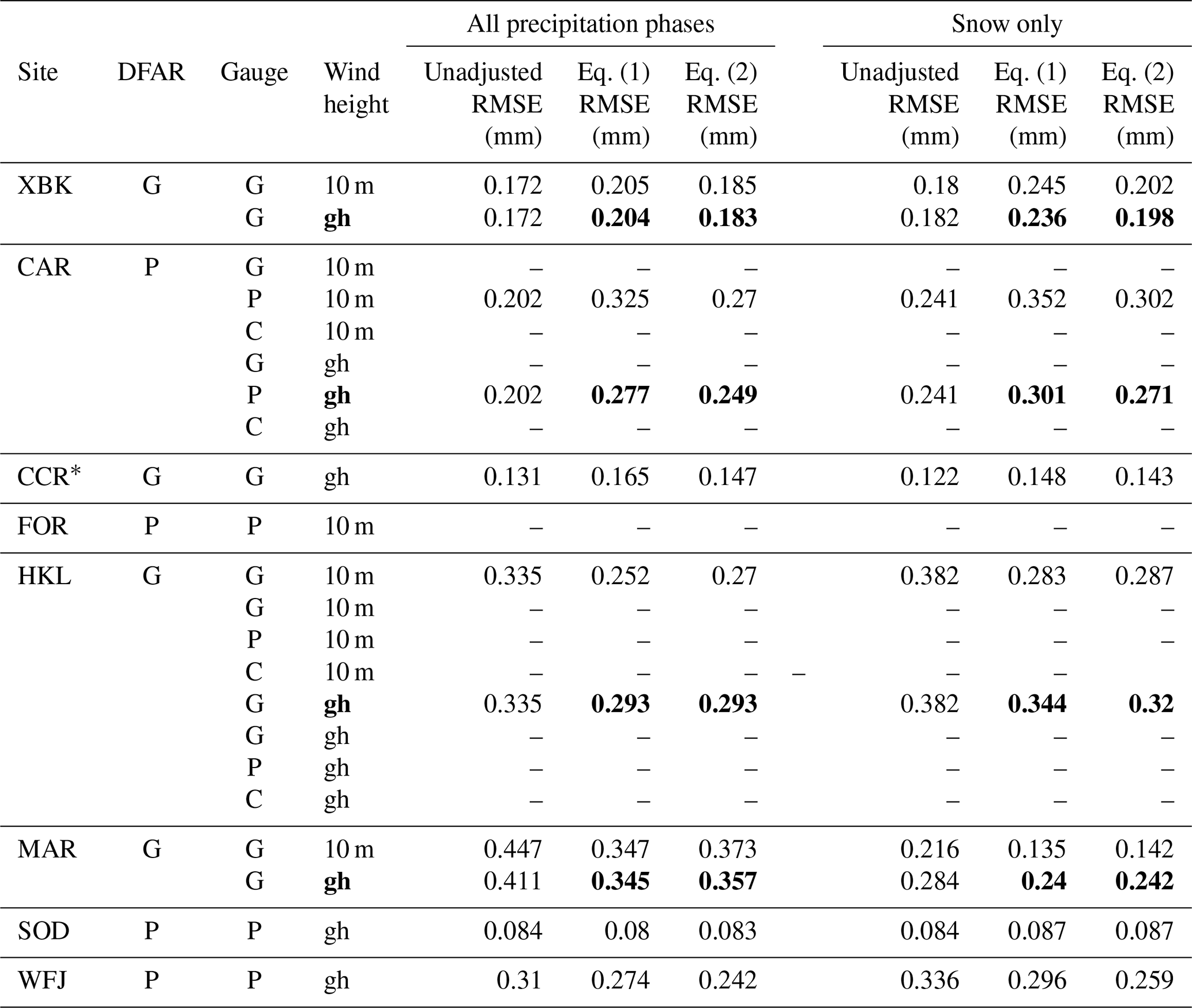
Table 3Relative total catch (RTC) for the unshielded gauges (G – Geonor; P – Pluvio2) as compared to the DFAR reference at each site for the combined winters of 2015/2016 and 2016/2017. Results are provided for available wind speed measurement heights (10 m; gh – gauge height) and for Eqs. (1) and (2). Metrics are separated by precipitation phase (all and snow only). Where both wind speed heights are available, the gauge height data are shown in bold.
* Indicates 2016/2017 winter only.
The RTC values in Tables 2 and 3 indicate that the unadjusted catch for snow is lower than the unadjusted catch for all precipitation types at most of the sites. The magnitude of the difference depends on the relative amounts of solid and liquid precipitation received during the season and the wind speeds during snow. The biggest difference in the unadjusted RTC values between all precipitation types and snow occurred at sites where more rain occurred during the intercomparison season, as the gauge catch for rainfall is naturally higher (Yang et al., 1998; Smith, 2008) and biases the total catch. At XBK, CAR, FOR, and HKL, removing rain and mixed precipitation from the statistics had a large impact on the RTC, both pre- and post-adjustment, and provided a more realistic metric for assessing how well the transfer functions were performing for the adjustment of snow measurements.
Although the sample size is smaller (fewer unshielded than single Alter-shielded gauges), the unadjusted catch of the unshielded gauges (Table 3) was lower than the unadjusted catch of the single Alter-shielded gauges (Table 2). From the single Alter-shielded RTC in Table 2, focusing on snow, the differences between Eqs. (1) and (2) results were small, varying within 1 % to 2 %. This can also be seen in the combined results in Fig. 5. The difference between Eqs. (1) and (2) was greater for the unshielded gauges (Table 3), with Eq. (1) performing better than Eq. (2) for snow at XBK (+12 %) and HKL (+10 % using Ugh). Equation (2) tended to under-adjust the unshielded gauges more than Eq. (1) at XBK and HKL.
At sites with both wind speed heights available for use in the adjustment (namely XBK, CAR, HKL, and MAR), the data shown in Table 2 for single Alter-shielded gauges suggest that using Ugh reduces the extent of over-adjustment (CAR and MAR) or under-adjustment (XBK and HKL) relative to U10 m (i.e. adjustments closer to 100 %). This holds for the unshielded gauge adjustments in Table 3 with the exception of MAR, which shows a large under-adjustment using Ugh as compared to U10 m. This may suggest that Ugh wind speeds are biased low at MAR, which is consistent with comments made by Kochendorfer et al. (2017a), who stated that the ground height wind measurement were shadowed in some directions. Although the sample size was small, there is reason to suggest, from an RTC perspective, that Ugh outperforms U10 m when used in Eqs. (1) and (2) for adjusting snow measurements. For this reason, where available, the Ugh rather than U10 m wind adjustments are shown in Fig. 5 and in subsequent figures.
The differences in RTC for the adjusted measurements from single Alter-shielded gauges versus those from unshielded gauges are mixed. At the windier HKL and XBK sites, Fig. 5 suggests that the adjusted RTC for the unshielded gauge is just as high as, or higher than, for the single Alter-shielded gauge (Eq. (2) at XBK being the exception). The over-adjustments at SOD and CCR are exaggerated for the unshielded gauge, but the unshielded adjustment is closer to 100 % at CAR and WFJ. MAR is an outlier in Fig. 5, possibly due to the potential issue with Ugh, but the U10 m adjustment of the unshielded gauge (Table 3; snow) has an RTC closer to 100 % (105 % and 106 % for Eqs. (1) and (2), respectively) than the single Alter-shielded gauge (117 %).
Including the RTC for both wind speed heights but excluding the combined gauge statistics, the adjustment for snow using Eq. (1) increases the mean catch efficiency for the single Alter-shielded gauge from 61 % to 88 % and for the unshielded gauge from 48 % to 92 %.
3.3 RMSE
Table 4 (single Alter-shielded gauges) and Table 5 (unshielded gauges) show the RMSE for each available SUT at each site and the RMSE when multiple SUTs are combined. As with RTC, the metric is provided for both transfer functions and using both wind speed heights where available.
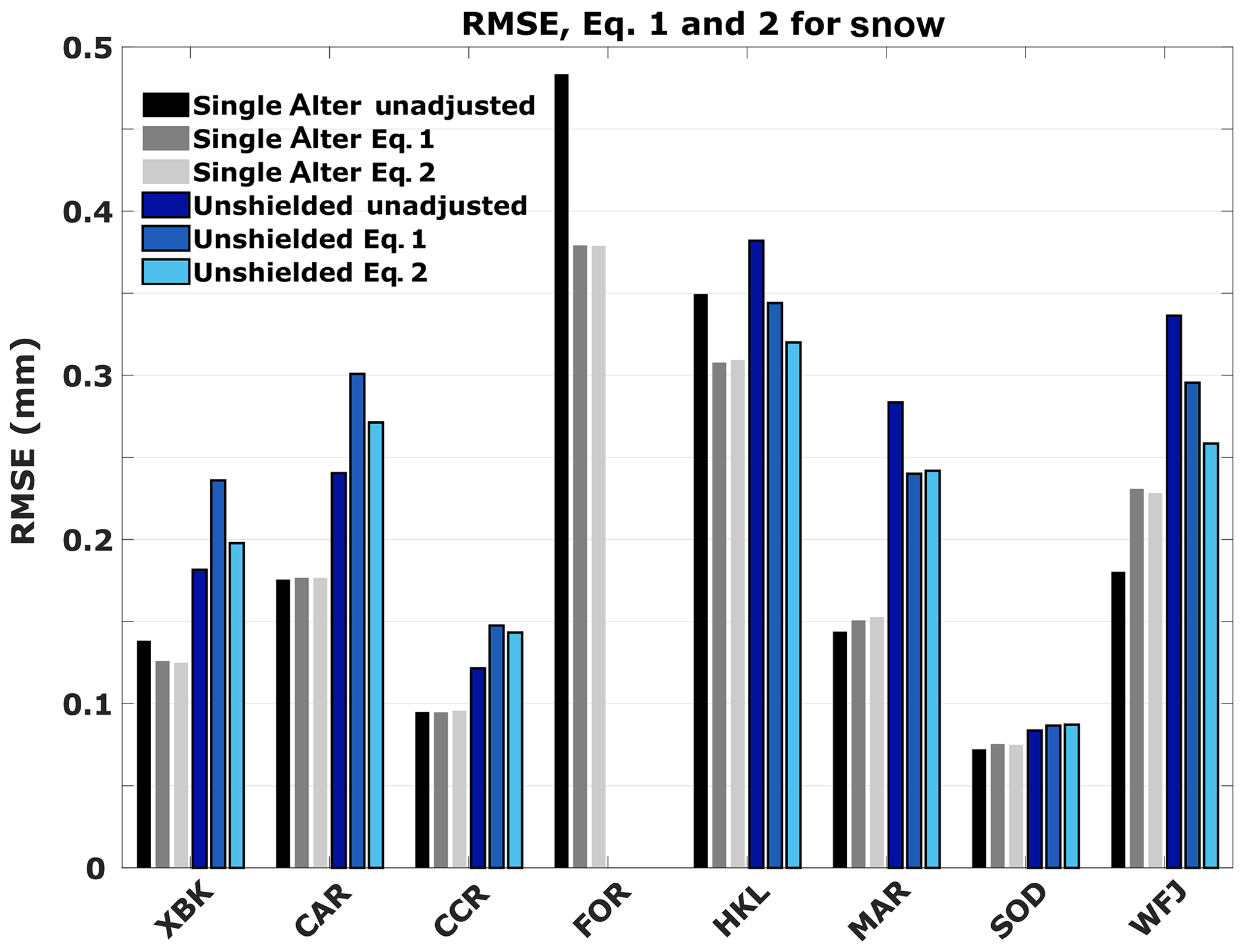
Figure 6Root mean square error (RMSE) for snow for single Alter and unshielded gauges for unadjusted measurements and for adjustments using Eqs. (1) and (2) at each of the eight SPICE sites, combining 2015/2016 and 2016/2017 winter seasons.
Comparing the RMSE values between Tables 4 and 5, the RMSE values for both the adjusted and unadjusted unshielded gauges are higher than their single Alter-shielded counterparts. However, the RMSE differences between all precipitation phases and those for snow are inconsistent, with RMSE occasionally being lower for snow than for all phases and vice versa. For the single Alter-shielded and unshielded gauges, respectively, 46 % and 36 % of the RMSE values are either lower or the same for snow as compared to all precipitation phases. The differences in adjusted RMSE with wind measurement height are also small. For single Alter-shielded gauges, CAR has a lower RMSE for Ugh, MAR has a higher RMSE for Ugh, and HKL and XBK show similar RMSE values for Ugh and U10 m. For unshielded gauges, the RMSE for Ugh is lower than that for U10 m at XBK and CAR, and higher at HKL and MAR.
When considering each gauge at each site, the anticipated decrease in the RMSE following the adjustment (whether for all precipitation types or snow only) is not universal. This is illustrated in Fig. 6 which shows the RMSE results for combined SUT snow data sets before and after the adjustment using U10 m (where possible). For single Alter-shielded gauges, the RMSE increases with the adjustment at CAR, MAR, SOD, and WFJ (although the increase is small at all sites but WFJ). The decrease in RMSE is small at XBK and CCR. The differences between RMSE results, using Eqs. (1) and (2), for single Alter-shielded gauges are insubstantial (<0.005 mm). These differences are larger for the unshielded gauges, as shown in Fig. 6 (as high as 0.05 mm).
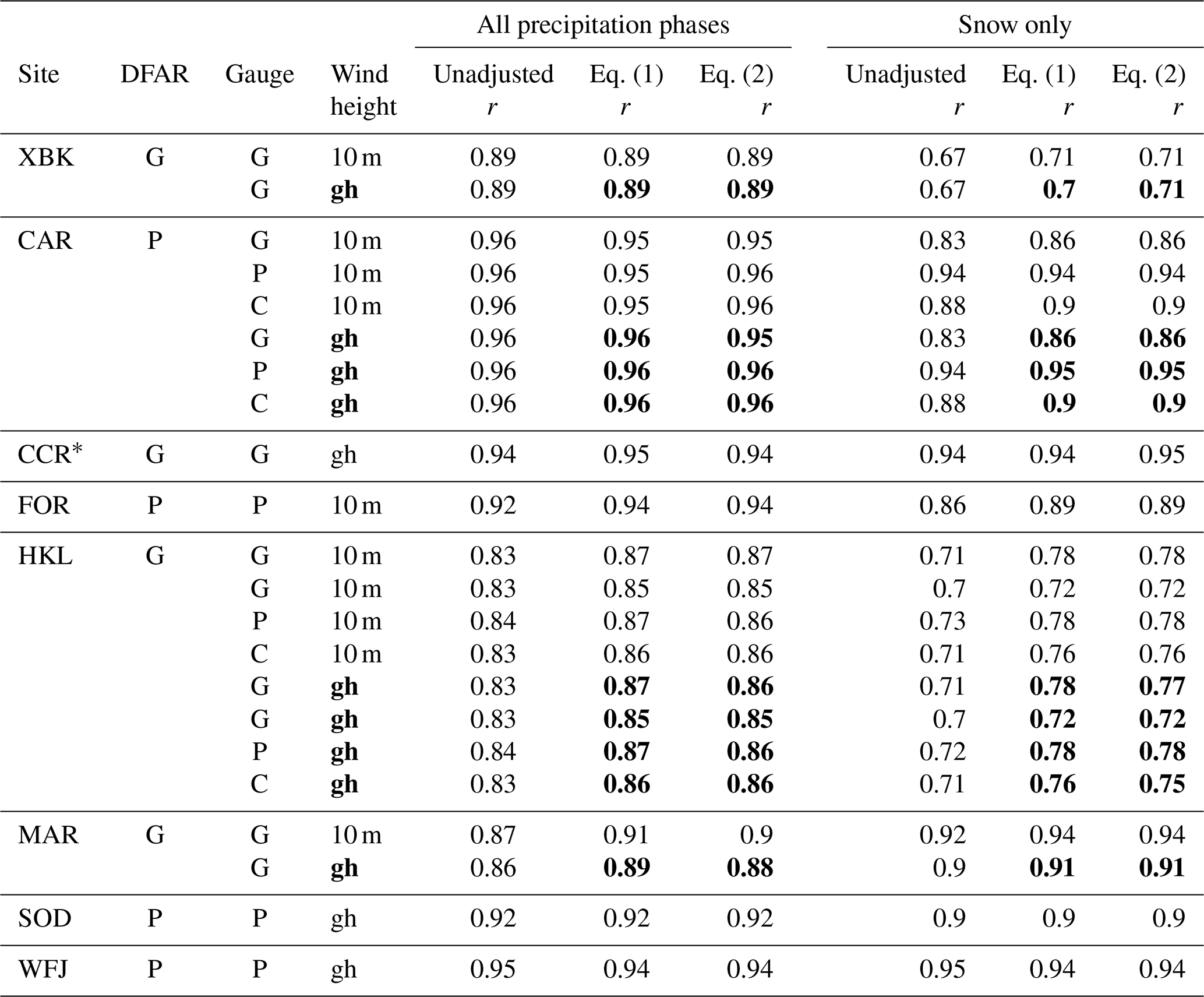
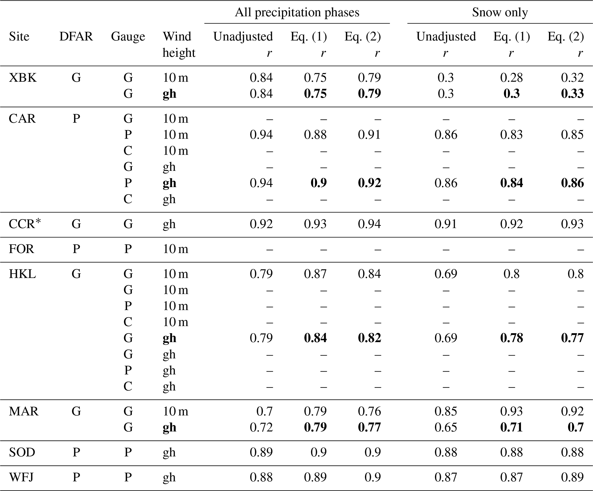
3.4 Pearson correlation
Similar to previous metrics, the single Alter-shielded and unshielded r values are shown separately in Tables 6 and 7, respectively, and are plotted for snow in Fig. 7. In theory, the adjustment using a transfer function should strengthen the linear relationship (increase r) between the adjusted and the reference measurements by removing the nonlinearity associated with wind bias.
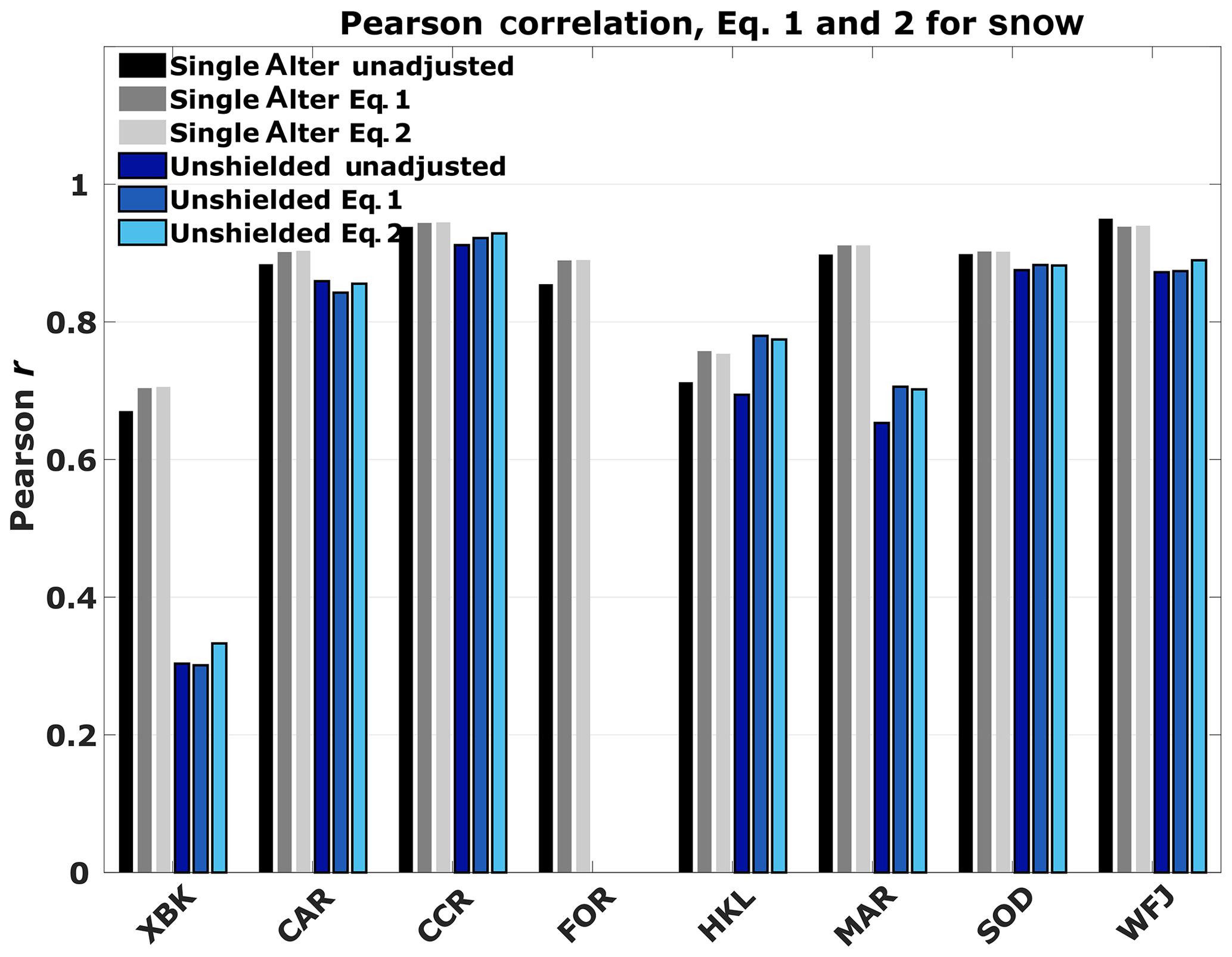
Figure 7Pearson r for single Alter and unshielded gauges for unadjusted measurements and for adjustments using Eqs. (1) and (2) at each of the eight SPICE sites, combining 2015/2016 and 2016/2017 winter seasons.
For single Alter-shielded gauges, unadjusted r values for all precipitation types range from 0.83 at HKL to 0.96 at CCR. For unshielded gauges, the unadjusted r values for all precipitation types are only slightly lower than their shielded counterparts. The unadjusted r values for single Alter-shielded gauges for snow are generally lower than for all precipitation types, especially at the windy sites of HKL and XBK. The unshielded, unadjusted values for snow follow similar trends to all precipitation types.
The results show that adjusting measurements for all precipitation types with either transfer function has little impact on the r values, with greater variability in r values observed for the unshielded gauges. The impact of adjustments on snow measurements are shown in Fig. 7. Generally, the r values for the single Alter-shielded gauges are improved with adjustment, but the change is small (<0.07). The largest improvements are observed for the HKL and XBK measurement data sets. With the unshielded adjustment, unshielded gauges at most sites also show an improvement in r values with adjustment, with the most significant increases observed for the HKL and MAR data sets.
For both all precipitation phases and snow only (Fig. 7), the differences between r values following the application of Eqs. (1) and (2) are negligible for the single Alter-shielded gauges. For the unshielded gauges, Eq. (2) results in higher r values than Eq. (1), but the differences are very small (<0.03).
For sites with both wind speed measurement heights, the correlations appear to be independent from the measurement height. The only exception is for the unshielded adjustment of snow measurements at MAR, where correlations based on the transfer function application using Ugh are significantly less than those using U10 m. This likely results from shadowing effects on the Ugh data.
3.5 Percentage of events within 0.1 mm
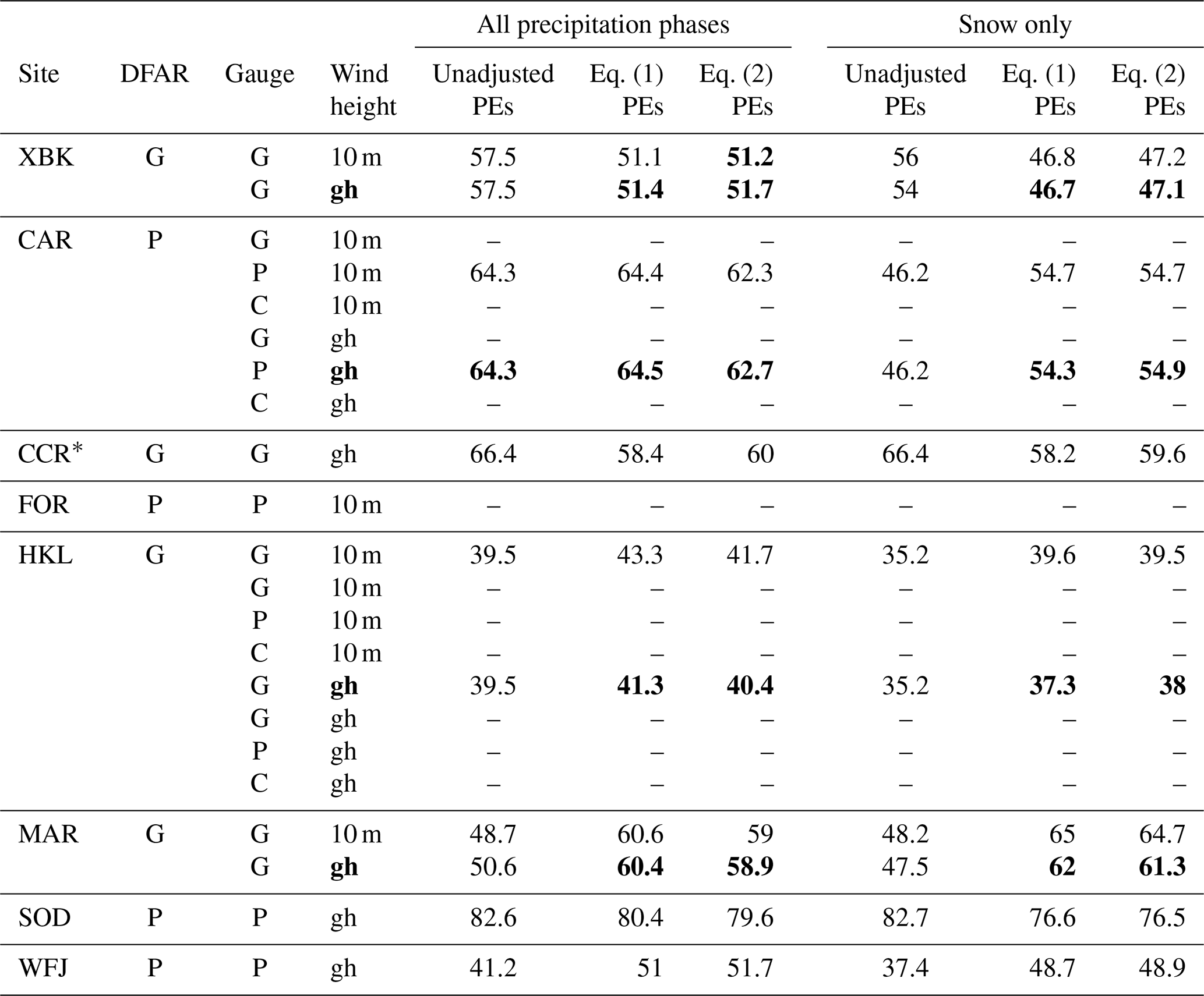
As shown in Table 8, the PEs for the single Alter-shielded gauges did not generally increase following adjustment, contrary to what was observed in K2017b. Similar to the observed trends for r and RMSE, the change in PEs following the adjustment of the Alter-shielded gauges was small, typically within ±5 %, with the only exception to this being at FOR (+10 % for snow).
Table 4Root mean square error (RMSE) for the single Alter-shielded gauges (G – Geonor; P – Pluvio2) as compared to the DFAR reference at each site for the combined winters of 2015/2016 and 2016/2017 for available wind speed measurement heights (10 m; gh – gauge height) and for Eqs. (1) and (2). Metrics are separated by precipitation phase (all and snow only). Where both wind speed heights are available, the gauge height data are shown in bold.
* Indicates 2016/2017 winter only.
Table 5Root mean square error (RMSE) for the unshielded gauges (G – Geonor; P – Pluvio2) as compared to the DFAR reference at each site for the combined winters of 2015/2016 and 2016/2017 for available wind speed measurement heights (10 m; gh – gauge height) and for Eqs. (1) and (2). Metrics are separated by precipitation phase (all and snow only). Where both wind speed heights are available, the gauge height data are shown in bold.
* Indicates 2016/2017 winter only.
Table 6Pearson correlation (r) for the single Alter-shielded gauges (G – Geonor; P – Pluvio2) as compared to the DFAR reference at each site for the combined winters of 2015/2016 and 2016/2017 for available wind speed measurement heights (10 m; gh – gauge height) and for Eqs. (1) and (2). Metrics are separated by precipitation phase (all and snow only). Where both wind speed heights are available, the gauge height data are shown in bold.
* Indicates 2016/2017 winter only.
Table 7Pearson correlation (r) for the unshielded gauges (G – Geonor; P – Pluvio2) as compared to the DFAR reference at each site for the combined winters of 2015/2016 and 2016/2017 for available wind speed measurement heights (10 m; gh – gauge height) and for Eqs. (1) and (2). Metrics are separated by precipitation phase (all and snow only). Where both wind speed heights are available, the gauge height data are shown in bold.
* Indicates 2016/2017 winter only.
Table 8Percentage of events (PEs) that differ from the DFAR by less than 0.1 mm for the single Alter-shielded gauges (G – Geonor; P – Pluvio2) at each site for the combined winters of 2015/2016 and 2016/2017 for available wind speed measurement heights (10 m; gh – gauge height) and for Eqs. (1) and (2). Metrics are separated by precipitation phase (all and snow only). Where both wind speed heights are available, the gauge height data are shown in bold.

* Indicates 2016/2017 winter only.
The unshielded gauges showed a greater change in PEs following the adjustment (Table 9). For all precipitation, the difference in PEs before and after the adjustment was generally small (MAR and FOR being the exceptions with a 10 % increase), but the change for snow was more substantial. As shown in Fig. 8, PEs for snow were found to decrease by more than 6 % at some sites following the adjustment (namely XBK, CCR, and SOD) and increase by more than 9 % at others (namely CAR, MAR, and WFJ), with changes varying between −8 % and +17 %.
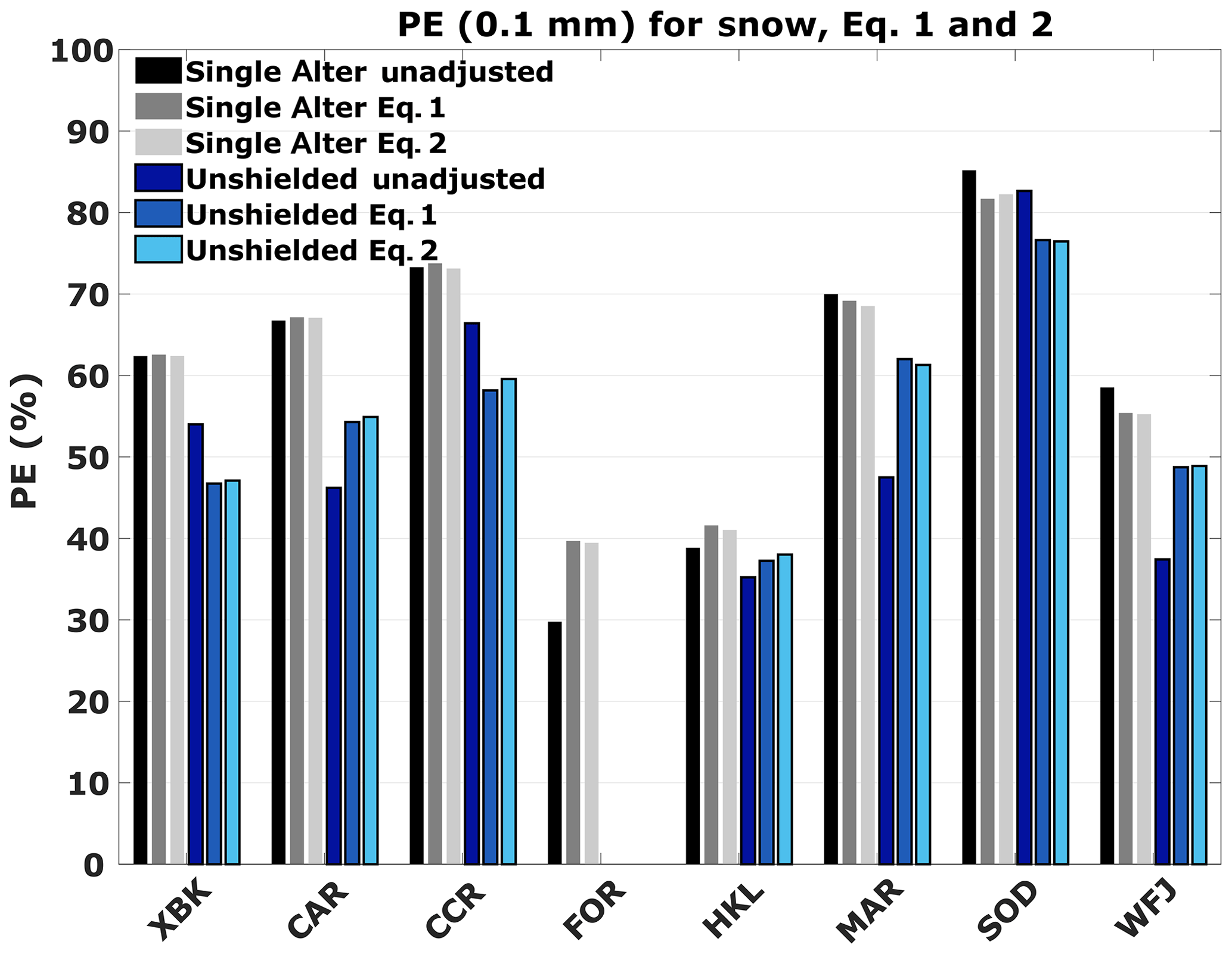
Figure 8Percentage of events (PEs) that differ from the DFAR by less than 0.1 mm for single Alter and unshielded gauges for unadjusted measurements and for adjustments using Eqs. (1) and (2) at each of the eight SPICE sites, combining 2015/2016 and 2016/2017 winter seasons.
Table 9Percentage of events (PEs) that differ from the DFAR by less than 0.1 mm for the unshielded gauges (G – Geonor; P – Pluvio2) at each site for the combined winters of 2015/2016 and 2016/2017 for available wind speed measurement heights (10 m; gh – gauge height) and for Eqs. (1) and (2). Metrics are separated by precipitation phase (all and snow only). Where both wind speed heights are available, the gauge height data are shown in bold.
* Indicates 2016/2017 winter only.
Similar to the other metrics, PEs do not show any consistent advantage to either Eq. (1) or Eq. (2), with differences being less than 2 % (most being less than 1 %). There also does not appear to be any clear or consistent advantage in using Ugh vs. U10 m, with differences in PE values generally within 2 %.
The current application of the universal transfer functions developed in SPICE to two winter seasons of precipitation data at eight locations produced variable results, depending on the site location. The discussion will focus on snow to avoid the complex influence of precipitation phases, in varying proportions, on the assessment results. Based on the relative total catch results, the transfer functions tend to under-adjust snow for single Alter-shielded gauges at the windy sites of XBK and HKL with a mean 10 m wind speed during snow of 6.1 and 5.3 m s−1, respectively (Table 2). The results from FOR were similar, despite relatively lower mean wind speeds of 4 m s−1 at 10 m. The SOD, CCR, WFJ, and MAR sites were characterized by the lowest wind speeds, with mean 10 m wind speed values lower than 3.2 m s−1. For single Alter-shielded gauges at these sites, the RTC, following the adjustment, varied from 105 % at SOD and CAR to 113 % at MAR and WFJ. The above trends are similar to the bias results of K2017b for all precipitation phases but are more pronounced due to the focus on snow.
The adjusted RTC results showed greater variability for unshielded gauges (Table 3), which performed better at some sites and worse at others relative to the performance for the single Alter-shielded gauges (Table 2). Similarly, variable trends were observed in the adjusted PE results for unshielded and Alter-shielded gauges (Tables 9 and 8, respectively). The adjustment of the unshielded gauges at the windy sites (XBK and HKL) was found to increase the RTC closer to 100 % than the adjustment for the Alter-shielded gauges; however, upon examination of the RMSE results (Fig. 6), the errors associated with adjusting the unshielded gauges were generally higher compared to those associated with the single Alter-shielded gauges. Insight into the higher RMSE values for unshielded gauges is provided by the PE results (Table 9 and Fig. 8). At XBK, the PEs dropped by 7 % after adjusting the unshielded gauge, indicating that more measurements were pushed outside of the ±0.1 mm threshold relative to the DFAR than were pushed inside the threshold by the adjustment. The PEs dropped after the adjustment for the unshielded gauges at CCR and SOD as well, but this can be attributed to over-adjustment, as shown by the RTC (Fig. 5). In summary, since the unadjusted RTC values for unshielded gauges are lower (especially at windy sites), the adjustments for unshielded measurements are necessarily larger, which magnifies signal noise and other random measurement errors. This propagation of errors through adjustment is discussed in greater detail by Kochendorfer et al. (2018).
The evaluation of transfer function performance is complicated by observations for which the DFAR detects a measurable amount of precipitation, but the SUT does not. A gauge measurement of zero cannot be adjusted with a transfer function. This impacts the performance metrics and cannot be ignored in the context of real-world applications of transfer functions (e.g. adjusting precipitation measurements for use in a forecast validation). The limited utility of transfer functions in this regard is due to the configuration's capability to catch snow and not because of the transfer function. To assess the relative impact of these types of events on the evaluations, descriptive statistics were calculated for events at XBK, HKL, and SOD.
For XBK, there were 498 30 min snow events during which the DFAR measured an accumulation value greater than 0. The single Alter-shielded gauge did not report precipitation during 285 of those events, which accounted for 14 % of the total DFAR accumulation over both measurement seasons, and had a mean wind speed of 6 m s−1 (7.5 m s−1) at gauge height (10 m). The number of events during which the unshielded gauge did not report precipitation was even higher, with 376 events in total, accounting for 24 % of the total DFAR precipitation, characterized by lower mean wind speeds (5.4 m s−1 at gauge height and 6.8 m s−1 at 10 m). For HKL, 860 of 1881 snow events were not reported by the single Alter-shielded gauge (8 % of the total DFAR accumulation), and 966 of the 1881 events were not reported by the unshielded gauge (10 % of the total DFAR accumulation). One can speculate that the influence of missed reports was more significant at XBK due to the drier nature of the site and of the falling snow, which made the snow more susceptible to deflection around the gauge inlet. At SOD, where wind speed has considerably less impact on gauge catch, 413 of 1656 events reported by DFAR were not reported by the single Alter-shielded gauge (about 6 % of the total DFAR accumulation). The number of occurrences for the unshielded gauge at SOD was nearly identical to the single Alter-shielded gauge. At windy sites, when precipitation goes undetected by a non-reference gauge, there is a negative impact on the transfer function performance metrics, but it also means that the effectiveness of the transfer function is reduced when it is applied to operational observations using those same gauge configurations. Since more shielding (e.g. double Alter) generally means a higher catch (Watson et al., 2008; Smith, 2009; Rasmussen et al., 2012; Kochendorfer et al., 2017b), more shielding would also reduce the number of unmeasured events. Perhaps another option for increasing the detection of small events in cold and windy locations would be the use of optical disdrometers paired with the conventional accumulating gauges.
Even though some adjusted RTC values are closer to 100 % for unshielded gauges (such as at HKL, CAR, and WFJ), the RMSE was generally lower and the PEs were consistently higher for single Alter-shielded gauges and, combined with a lower frequency of missed measurements, supports the use of more shielding for solid precipitation measurements.
In general, the application of transfer functions resulted in under-adjustment at the windier sites and over-adjustment at the less windy sites; however, there is no clear relationship between the mean wind speed at a site and transfer function performance. The general performance of the transfer functions for single Alter-shielded gauge measurements, from the perspective of RTC, likely also depends on other factors, such as crystal characteristics (Thériault et al., 2012) or aerodynamic peculiarities at the intercomparison sites affecting the representative wind speed measurements (as discussed in K2017b). Based on the present results, we found that the transfer function performance varied by site, and the windy sites were under-adjusted while the less windy sites were over-adjusted, but the magnitude of the adjustment error and the specific causes of error were difficult to determine. Although beyond the scope of this work, an alternative to universal transfer functions may be to develop site-specific transfer functions. Applicability to other sites with similar conditions could be assessed using a site-classification process based on climate parameters and principle components analysis, such as those shown in Pierre et al. (2019).
The differences in performance between Eqs. (1) and (2) for adjusting snow measurements from single Alter-shielded gauges were small in that RTC generally varied by less than 2 % and RMSE, r, and PEs were nearly identical. This was likely an artefact of the way that phase was determined in the methodology; even though CE is a function of air temperature in Eq. (1), the data for snow are a subset of the precipitation data based on the same phase discrimination used for Eq. (2). However, the metrics for all precipitation types were also similar, which is consistent with the results in K2017b, and suggests that transfer function selection is essentially a matter of user preference. In that respect, the “simpler” Eq. (2) is less simple in that user is required to determine the phase based on temperature thresholds, while Eq. (1) requires no phase discrimination. The decision would appear to be more complicated for unshielded gauges, likely because of the increased uncertainty in both the measurement and the adjustment. Generally, the differences are still quite small, but Eq. (2) shows a slight advantage with RMSE and r. As with the single Alter-shielded gauges, the decision likely should be based on personal preference. It would be interesting, however, to explore refining the coefficients for Eq. (2), using optical disdrometers or present weather sensors to identify the dominant precipitation phase, and employ such instruments when performing adjustments. It may also be worthwhile to assess the performance of Eq. (2) while using hydrometeor temperature approximation, as described in Harder and Pomeroy (2013), for phase discrimination.
Only four of the eight test sites measured both U10 m and Ugh, so it is difficult to draw conclusions regarding the influence of wind speed measurement height on the performance of the transfer functions. For those four sites, the RTC using Ugh was closer to 100 % for many of the adjustments, but RMSE and PEs varied by site and r values were nearly identical. The Ugh is a direct measurement of the wind speed at gauge height and does not rely on the potentially problematic assumption that wind speed at 10 m is representative of wind speed at gauge height. This assumption relies on the estimation of surface roughness, which changes with vegetation cover, snowfall, and drifting. It also neglects the impact of increasing snow depth on the relationship between the gauge height wind speed and the 10 m height wind speed. However, depending on the distance between the SUT and the Ugh measurement, the Ugh measurement may also not be representative of the wind speed at the SUT due to interference from instruments, wind shields, and other obstructions between the wind sensor and the gauge.
As noted in K2017b, discrepancies in the various wind speed measurements (whether instrument, height, or exposure related) make it difficult to ascertain any advantage or disadvantage of using one wind speed height over the other. It is recommended that the best wind speed data available at a given site are used for transfer function adjustment but to be cognisant of the issues related to the spatial representation of wind speed at the site. Additional uncertainty related to wind speed may be attributed to the variability within the 30 min mean period. Although this was not included in the current analysis, previous work by Wolff et al. (2015) and Nitu et al. (2018) at HKL showed that the impact of high-frequency variability in the wind speed over 30 min periods on transfer functions was negligible.
The evaluation of the performance of WMO-SPICE transfer functions using an independent, post-SPICE data set showed that the performance varies by site and shield configuration and is considerably reduced when only assessing their performance for snow. Generally, the application of the transfer functions to measurements from sites with higher wind speeds resulted in an under-adjustment, while producing an over-adjustment for measurements from less windy sites. This trend was not universal, which indicates that the performance is also linked to local climatic conditions affecting snowfall characteristics. On average, the transfer functions resulted in an increase in the RTC of snow measurements from single Alter-shielded gauges (unshielded gauges) from 61 % (48 %) to 88 % (92 %), but they also produced an under-adjustment as low as 54 % and an over-adjustment as high as 123 %. Although the RTC values imply improved transfer function performance when adjusting unshielded gauges relative to single Alter-shielded gauges, the higher RMSE and lower PEs for unshielded adjustments suggest otherwise. Furthermore, the unshielded gauges were shown to completely miss a larger proportion of events and accumulated precipitation relative to the DFAR than the shielded gauges, raising the critical point that precipitation that is not recorded by the gauge configuration cannot be adjusted. The differences in performance observed for Eqs. (1) and (2) were small enough that the choice of transfer function should largely depend on the availability of observed precipitation-phase data and user preference. With only four sites collecting wind speed data at both 10 m and gauge height, it was difficult to determine if the wind speed measurement height significantly affected transfer function performance. RTC was generally closer to 100 % when gauge height winds were used for the adjustment, but the RMSE, PEs, and correlation results were mixed. Regardless, and perhaps more importantly, users must also carefully consider potential issues with obstructions and spatial representativeness when selecting a wind speed measurement.
Ultimately, eight DFAR intercomparison sites were insufficient to address the variability in performance of the SPICE transfer functions, and more intercomparison sites with a DFAR are needed in various cold region climate regimes for more thorough assessments, which is a key recommendation from the WMO-SPICE project (Nitu et al., 2018). For the most part, and especially at locations that experience relatively high wind speeds during snowfall events, the application of the adjustment improved the usability of the observations. This study also suggests a high degree of uncertainty in applying these adjustments in networks that geographically span many different climate regimes, and additional work is required to assess and minimize that uncertainty.
The quality-controlled 30 min data set used in this publication is available at https://doi.org/10.1594/PANGAEA.907379 (Smith et al., 2019b).
CS is the lead author and completed the bulk of the analysis. AR was responsible for the data management, including coding, quality control, and processing. JK provided advice and expertise on the use and assessment of transfer functions. ME provided advice on the analysis and paper development and contributed to the design and implementation of the WMO-SPICE data and quality control procedures used on these data. JK, ME, MW, SB, YR, TL, and CS were core participants of the WMO-SPICE data team and were instrumental in the collection and provision of these data.
The authors declare that they have no conflict of interest.
The authors would like to thank Eva Mekis of Environment and Climate Change Canada for providing an internal review of this paper. We would like to acknowledge the following organizations that collected and provided the data for these analyses: Environment and Climate Change Canada (Climate Research Division and the Meteorological Service of Canada Observing Systems and Engineering) for XBK, CAR, and CCR; the National Center for Atmospheric Research and the National Oceanic and Atmospheric Administration for MAR; the Norwegian Meteorological Institute for HKL; MeteoSwiss for WFJ; the Finnish Meteorological Institute for SOD; and the Spanish National Meteorological Agency for FOR. Lastly, we would like to extend our gratitude to the two anonymous reviewers who provided insightful comments and suggestions that resulted in the improvement of this paper.
This paper was edited by Jan Seibert and reviewed by two anonymous referees.
Buisán, S. T., Earle, M. E., Collado, J. L., Kochendorfer, J., Alastrué, J., Wolff, M., Smith, C. D., and López-Moreno, J. I.: Assessment of snowfall accumulation underestimation by tipping bucket gauges in the Spanish operational network, Atmos. Meas. Tech., 10, 1079–1091, https://doi.org/10.5194/amt-10-1079-2017, 2017.
Førland, E. J. and Hanssen-Bauer, I.: Increased Precipitation in the Norwegian Arctic: True or False?, Climatic Change, 46, 485–509, https://doi.org/10.1023/A:1005613304674, 2000.
Goodison, B., Louie, P., and Yang, D.: The WMO solid precipitation measurement intercomparison, WMO/TD No. 872, World Meteorological Organization Publications, Geneva, 1998.
Goodison, B. E.: Accuracy of Canadian snow gauge measurements, J. Appl. Meteorol., 17, 1542–1548, 1978.
Harder, P. and Pomeroy, J.: Estimating precipitation phase using a psychrometric energy balance method, Hydrol. Process., 27, 1901–1914, https://doi.org/10.1002/hyp.9799, 2013.
Kochendorfer, J., Rasmussen, R., Wolff, M., Baker, B., Hall, M. E., Meyers, T., Landolt, S., Jachcik, A., Isaksen, K., Brækkan, R., and Leeper, R.: The quantification and correction of wind induced precipitation measurement errors, Hydrol. Earth Syst. Sci., 21, 1973–1989, https://doi.org/10.5194/hess-21-1973-2017, 2017a.
Kochendorfer, J., Nitu, R., Wolff, M., Mekis, E., Rasmussen, R., Baker, B., Earle, M. E., Reverdin, A., Wong, K., Smith, C. D., Yang, D., Roulet, Y.-A., Buisán, S., Laine, T., Lee, G., Aceituno, J. L. C., Alastrué, J., Isaksen, K., Meyers, T., Brækkan, R., Landolt, S., Jachcik, A., and Poikonen, A.: Analysis of single-Alter-shielded and unshielded measurements of mixed and solid precipitation from WMO-SPICE, Hydrol. Earth Syst. Sci., 21, 3525–3542, https://doi.org/10.5194/hess-21-3525-2017, 2017b.
Kochendorfer, J., Nitu, R., Wolff, M., Mekis, E., Rasmussen, R., Baker, B., Earle, M. E., Reverdin, A., Wong, K., Smith, C. D., Yang, D., Roulet, Y.-A., Meyers, T., Buisan, S., Isaksen, K., Brækkan, R., Landolt, S., and Jachcik, A.: Testing and development of transfer functions for weighing precipitation gauges in WMO-SPICE, Hydrol. Earth Syst. Sci., 22, 1437–1452, https://doi.org/10.5194/hess-22-1437-2018, 2018.
Nitu, R., Rasmussen, R., Baker, B., Lanzinger, E., Joe, P., Yang, D., Smith, C., Roulet, Y., Goodison, B., Liang, H., Sabatini, F., Kochendorfer, J., Wolff, M., Hendrikx, J., Vuerich, E., Lanza, L., Aulamo, O., and Vuglinsky, V.: WMO intercomparison of instruments and methods for the measurement of solid precipitation and snow on the ground: organization of the experiment, in: WMO Technical Conference on meteorological and environmental instruments and methods of observations, Brussels, Belgium, 16–18, 2012.
Nitu, R., Rasmussen, R., and Roulet, Y.: WMO SPICE: Intercomparison of instruments and methods for the measurement of solid precipitation and snow on the ground, overall results and recomendations, in: WMO Technical Conference on meteorological and environmental instruments and methods of observations, Madrid, Spain, 1–7, available at: https://www.wmo.int/pages/prog/www/IMOP/publications/IOM-125_TECO_2016/Session_3/K3A_Nitu_SPICE.pdf (last access: July 2018), 2016.
Nitu, R., Roulet, Y.-A., Wolff, M., Earle, M., Reverdin, A., Smith, C., Kochendorfer, J., Morin, S., Rasmussen, R., Wong, K., Alastrué, J., Arnold, L., Baker, B., Buisán, S., Collado, J. L., Colli, M., Collins, B., Gaydos, A., Hannula, H.-R., Hoover, J., Joe, P., Kontu, A., Laine, T., Lanza, L., Lanzinger, E., Lee, G. W., Lejeune, Y., Leppänen, L., Mekis, E., Panel, J.-M., Poikonen, A., Ryu, S., Sabatini, F., Theriault, J., Yang, D., Genthon, C., van den Heuvel, F., Hirasawa, N., Konishi, H., Nishimura, K., and Senese, A.: WMO Solid Precipitation Intercomparison Experiment (SPICE) (2012–2015), Instruments and Observing Methods Report No. 131, World Meteorological Organization, Geneva, 2018.
Pan, X., Yang, D., Li, Y., Barr, A., Helgason, W., Hayashi, M., Marsh, P., Pomeroy, J., and Janowicz, R. J.: Bias corrections of precipitation measurements across experimental sites in different ecoclimatic regions of western Canada, The Cryosphere, 10, 2347–2360, https://doi.org/10.5194/tc-10-2347-2016, 2016.
Pierre, A., Jutras, S., Smith, C., Kochendorfer, J., Fortin, V., Anctil, F.: Evaluation of catch efficiency transfer functions for unshielded and single-Alter-shielded solid precipitation measurements, J. Atmos. Ocean. Tech., 36, 865–881, https://doi.org/10.1175/JTECH-D-18-0112.1, 2019.
Rasmussen, R. M., Baker, B., Kochendorfer, J., Myers, T., Landolt, S., Fisher, A., Black, J., Theriault, J., Kucera, P., Gochis, D. J., Smith, C., Nitu, R., Hall, M., Cristanelli, S., and Gutmann, E.: How Well Are We Measuring Snow? The NOAA/FAA/NCAR Winter Precipitation Test Bed, B. Am. Meteorol. Soc., 93, 811–829, 2012.
Reverdin, A.: Description of the Quality Control and Event Selection Procedures used within the WMO-SPICE project, in: WMO Technical Conference on meteorological and environmental instruments and methods of observations, Madrid, Spain, available at: https://www.wmo.int/pages/prog/www/IMOP/publications/IOM-125_TECO_2016/Session_3/P3(10)_Reverdin.pdf (last access: August 2020), 2016.
Scaff, L., Yang, D., Li, Y., and Mekis, E.: Inconsistency in precipitation measurements across the Alaska–Yukon border, The Cryosphere, 9, 2417–2428, https://doi.org/10.5194/tc-9-2417-2015, 2015.
Sevruk, B., Hertig, J.-A., and Spiess, R.: The effect of a precipitation gauge orifice rim on the wind field deformation as investigated in a wind tunnel, Atmos. Environ. A, 25, 1173–1179, 1991.
Sevruk, B., Ondras, M., and Chvila, B.: The WMO precipitation measurement intercomparisons, Atmos. Res., 92, 376–380, 2009.
Smith, C. D.: Correcting the wind bias in snowfall measurements made with a Geonor T-200B precipitation gauge and Alter wind shield, CMOS Bulletin SCMO, 36, 162–167, 2008.
Smith, C. D.: The relationship between snowfall catch efficiency and wind speed for the Geonor T-200B precipitation gauge utilizing various wind shield configurations, 20–23 April 2009, Canmore, Alberta, 115–121, 2009.
Smith, C. D., Yang, D., Ross, A., and Barr, A.: The Environment and Climate Change Canada solid precipitation intercomparison data from Bratt's Lake and Caribou Creek, Saskatchewan, Earth Syst. Sci. Data, 11, 1337–1347, https://doi.org/10.5194/essd-11-1337-2019, 2019a.
Smith, C. D., Ross, A., Kochendorfer, J., Earle, M. E., Wolff, M., Buisán, S., Roulet, Y., and Laine, T.: The Post-SPICE (2015/2016 and 2016/2017) Winter Precipitation Intercomparison Data. PANGAEA, https://doi.org/10.1594/PANGAEA.907379, 2019b.
Thériault, J. M., Rasmussen, R., Ikeda,K., and Landolt, S.: Dependence of snow gauge collection efficiency on snowflake characteristics, J. Appl. Meteorol. Clim., 51, 745–762, https://doi.org/10.1175/JAMC-D-11-0116.1, 2012.
Watson, S., Smith, C., Lassi, M., and Misfeldt, J.: An evaluation of the effectiveness of the double-Alter wind shield for increasing the catch efficiency of the Geonor T-200B precipitation gauge, Can. Meteorol. Oceanogr. Soc. Bull., 36, 168–175, 2008.
Wolff, M. A., Isaksen, K., Petersen-Øverleir, A., Ødemark, K., Reitan, T., and Brækkan, R.: Derivation of a new continuous adjustment function for correcting wind-induced loss of solid precipitation: results of a Norwegian field study, Hydrol. Earth Syst. Sci., 19, 951–967, https://doi.org/10.5194/hess-19-951-2015, 2015.
Yang, D. and Ohata, T.: A bias-corrected Siberian regional precipitation climatology, J. Hydrometeorol., 2, 122–139, https://doi.org/10.1175/1525-7541(2001)002<0122:ABCSRP>2.0.CO;2, 2001.
Yang, D., Metcalfe, J. R., Goodison, B. E., and Mekis, E.: True SNOWfall. An evaluation of the double fence intercomparison reference gauge, in: 50th Eastern SNOW Conference and 61st Western SNOW Conference, Quebec City, 105–111, 1993.
Yang, D., Goodison, B. E., Metcalfe, J. R., Golubev, V. S., Bates, R., Pangburn, T., and Hanson, C. L.: Accuracy of NWS 8′′ standard nonrecording precipitation gauge: Results and application of WMO intercomparison, J. Atmos. Ocean. Tech., 15, 54–68, https://doi.org/10.1175/1520-0426(1998)015<0054:AONSNP>2.0.CO;2, 1998.