the Creative Commons Attribution 4.0 License.
the Creative Commons Attribution 4.0 License.
 | 18 Aug 2020
New model of reactive transport in a single-well push–pull test with aquitard effect and wellbore storage
Junxia Wang
Hongbin Zhan
Wenguang Shi
The model of single-well push–pull (SWPP) test has been widely used to investigate reactive radial dispersion in remediation or parameter estimation of in situ aquifers. Previous analytical solutions only focused on a completely isolated aquifer for the SWPP test, excluding any influence of aquitards bounding the tested aquifer, and ignored the wellbore storage of the chaser and rest phases in the SWPP test. Such simplification might be questionable in field applications when test durations are relatively long because solute transport in or out of the bounding aquitards is inevitable due to molecular diffusion and cross-formational advective transport. Here, a new SWPP model is developed in an aquifer–aquitard system with wellbore storage, and the analytical solution in the Laplace domain is derived. Four phases of the test are included: the injection phase, the chaser phase, the rest phase and the extraction phase. As the permeability of the aquitard is much smaller than the permeability of the aquifer, the flow is assumed to be perpendicular to the aquitard; thus only vertical dispersive and advective transports are considered for the aquitard. The validity of this treatment is tested against results grounded in numerical simulations. The global sensitivity analysis indicates that the results of the SWPP test are largely sensitive (i.e., influenced by) to the parameters of porosity and radial dispersion of the aquifer, whereas the influence of the aquitard on results could not be ignored. In the injection phase, the larger radial dispersivity of the aquifer could result in the smaller values of breakthrough curves (BTCs), while there are greater BTC values in the chaser and rest phases. In the extraction phase, it could lead to the smaller peak values of BTCs. The new model of this study is a generalization of several previous studies, and it performs better than previous studies ignoring the aquitard effect and wellbore storage for interpreting data of the field SWPP test reported by Yang et al. (2014).
- Article
(2465 KB) - Full-text XML
-
Supplement
(757 KB) - BibTeX
- EndNote


A single-well push–pull (SWPP) test could be applied for investigating aquifer properties related to reactive transport in the subsurface instead of the inter-well tracer test, due to its advantages of efficiency, low cost and easy implementation. The SWPP test is sometimes called the single-well injection–withdrawal test, single-well huff–puff test or single-well injection–backflow test (Jung and Pruess, 2012). A complete SWPP test includes the injection, the chaser, the rest and the extraction phase. The second and third phases are generally ignored in the analytical solutions but recommended in the field applications, since they could increase the reaction time for the injected chemicals with the porous media (Phanikumar and McGuire, 2010; Wang and Zhan, 2019).
Similar to other aquifer tests, the SWPP test is a forced-gradient groundwater tracer test, and analytical solutions are often preferred to determine the in situ aquifer properties, due to the computational efficiency. Currently, many analytical models are available for various scenarios of the SWPP tests (Gelhar and Collins, 1971; Huang et al., 2010; Chen et al., 2017; Schroth and Istok, 2005; Wang et al., 2018). However, these studies are based on a common underlying assumption, i.e., that the studied aquifer was isolated from adjacent aquitards. In other words, the aquitards bounding the aquifer are taken as two completely impermeable barriers for solute transport. To date, numerous studies have demonstrated that such an assumption might cause errors for groundwater flow (Zlotnik and Zhan, 2005; Hantush, 1967) and for reactive transport (Zhan et al., 2009; Chowdhury et al., 2017; Li et al., 2019). This is because even without any flow in the aquitards, molecular diffusion inevitably occurs when solute injected to the aquifer is close to the aquitard–aquifer interface. This is particularly true when a fully penetrating well is used for injection; thus a portion of injected solute is very close to the aquitard–aquifer interface and the SWPP test duration is relatively long, so the effect of molecular diffusion can materialize. Another important point to note is that the materials of the aquitard are usually clay and silt, which have strong absorbing capability for chemicals and great mass storage capacities (Chowdhury et al., 2017). To date, the influence of the aquitard on reactive transport in aquifers has attracted attention for several decades. As for radial dispersion, Chen (1985), Wang and Zhan (2013), and Zhou et al. (2017) presented analytical solutions for radial dispersion around an injection well in an aquifer–aquitard system. However, these models only focus on the first phase of the SWPP test (injection).
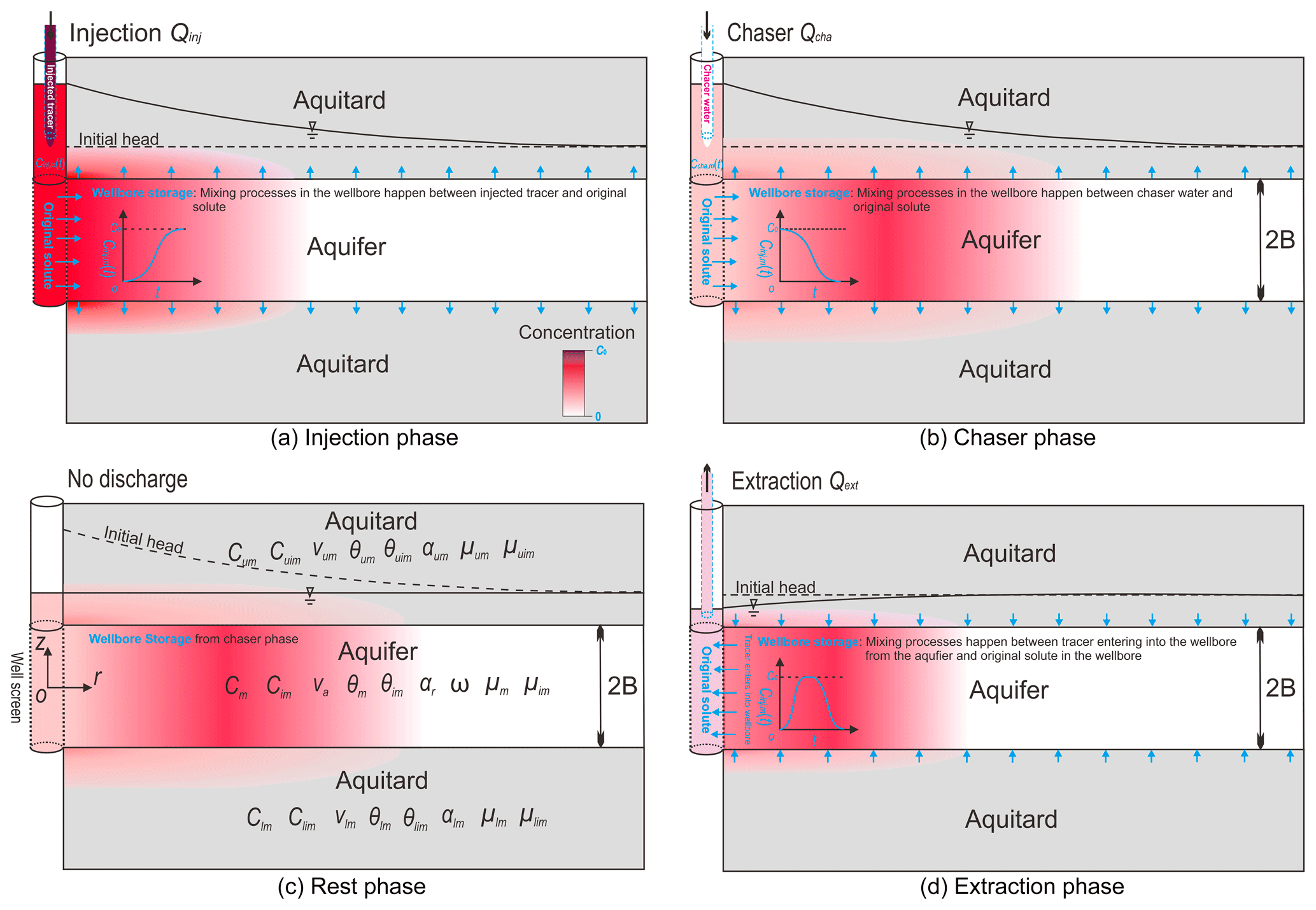
Another assumption included in many previous models of radial dispersion is that the wellbore storage is ignored for the solute transport. In the injection phase of the SWPP test, the wellbore storage refers to the mixing processes between the prepared tracer injected into the wellbore and the original (or native) water in the wellbore. As a result of the wellbore storage, the concentration inside the wellbore varies with time until reaching the same value as the injected concentration, as shown in Fig. 1a. When ignoring it, the concentration inside the wellbore is constant during the entire inject phase, which is certainly not true. Similarly, the wellbore storage in the chaser, rest and extraction phases refers to the concentration variation caused by mixing processes between the original solute in the wellbore and the tracer moving in or out the wellbore. The examples of ignoring wellbore storage include Gelhar and Collins (1971), Chen (1985, 1987), Moench (1989), Chen et al. (2007, 2012, 2017), Schroth et al. (2001), Tang and Babu (1979), Huang et al. (2010) and Zhou et al. (2017). Recently, Wang et al. (2018) developed a two-phase (injection and extraction) model for the SWPP test with specific considerations of the wellbore storage. In many field applications, the chaser and rest phases are generally involved and the mixing effect also happens in these two phases in the SWPP test, which will be investigated in this study.
Besides the abovementioned issues in previous studies, another issue is that the advection–dispersion equation (ADE) was used to govern the reactive transport of SWPP tests (Gelhar and Collins, 1971; Wang et al., 2018; Jung and Pruess, 2012). The validity of ADE has been challenged by numerous laboratory and field experimental studies before, when using a single representative value of advection, dispersion and reaction to characterize the whole system. In a hypothetical case, if great details of heterogeneity are known, one may employ a sufficiently fine mesh to discretize the porous media of concern and use ADE to capture anomalous transport characteristics fairly well (e.g., the early arrivals and/or heavy late-time tails of the breakthrough curves, BTCs). However, such a hypothetical case has rarely materialized in real applications, especially for field-scale problems. To remedy the situation (at least to some degree), the multi-rate mass transfer (MMT) model was proposed as an alternative to interpret the data of the SWPP test (Huang et al., 2010; Chen et al., 2017). In the MMT model, the porous media is divided into many overlapping continuums (Haggerty et al., 2000; Haggerty and Gorelick, 1995). A subset of MMT is the two overlapping continuums or the mobile–immobile model (MIM) in which the mass transfer between two domains (mobile and immobile) becomes a single parameter instead of a function. The MIM model can grasp most characteristics of MMT and is mathematically simpler than MMT. Besides the MMT model, the continuous time random walk (CTRW) model and the fractional advection–dispersion equation (FADE) model were also applied for anomalous reactive transport in SWPP tests (Hansen et al., 2017; Chen et al., 2017). Due to the complexity of the mathematic models of CTRW and FADE, it is very difficult or even impossible to derive analytical solutions for those two models, although both methods perform well in a numerical framework.
In this study, a new model of SWPP tests will be established by including both wellbore storage and the aquitard effect under the MIM framework. The reason for choosing MIM as the working framework is to capture the possible anomalous transport characteristics that cannot be described by ADE but at the same time to make the analytical treatment of the problem possible. Four stages of a SWPP test will be considered. The model of the wellbore storage will be developed using a mass balance principle in the chaser and rest phases. It does not seem difficult to solve this model of this study using numerical packages like MODFLOW-MT3DMS, TOUGH and TOUGHREACT, and FEFLOW. However, the numerical solutions may cause errors in treating the wellbore storage, since the volume of water in the wellbore was assumed to be constant (Wang et al., 2018), while in reality it changes with time and well discharge. Meanwhile, the numerical errors (like numerical dispersion and numerical oscillation) have to be considered in solving the ADE equation, especially for advection-dominated transport. In this study, an analytical solution will be derived to facilitate the data interpretation. Due to the format of analytical solutions, it is much easier to couple such solutions with a proper optimization algorithm (like a genetic algorithm). The analytical solution could serve as a benchmark to test the numerical solutions as well.
A single test well is assumed to fully penetrate an aquifer with uniform thickness. Both the aquifer and aquitards are homogeneous and extend laterally to infinity. Linear sorption and first-order degradation are included in the mathematic model of the SWPP test. Such assumptions might be oversimplified for cases in reality, while they are inevitable for the derivation of the analytical solution, especially for the aquifer homogeneity. For a heterogeneity aquifer, the solution presented here may be regarded as an ensemble-averaged approximation if the heterogeneity is spatially stationary. If the heterogeneity is spatially non-stationary, then one can apply non-stationary stochastic approach and/or Monte Carlo simulations to deal with the issue, which is out of the scope of this investigation.
The concept of homogeneity here deserves clarification. Despite the fact that the homogeneity assumption is commonly used in developing analytical and numerical models of subsurface flow and transport, one should be aware that a rigorous sense of homogeneity probably never exists in a real-world setting (unless the media are composed of idealized glass balls as in some laboratory experiments). Therefore, the homogeneity concept here should be envisaged as a media whose hydraulic parameters vary within relatively narrow ranges, or the so-called weak heterogeneity. The Borden site of Canada (Sudicky, 1988) is one example of weak aquifer heterogeneity. Wang et al. (2018) employed a stochastic modeling technique to test the assumption of homogeneity associated with the SWPP test and found that such an assumption could be used to approximate a heterogeneous aquifer when the variance of spatial hydraulic conductivity was small.
A cylindrical coordinate system is employed in this study, and the origin is located at the well center, as shown in Fig. 1c. The z axis and the r axis are vertical and horizontal, respectively. Figure 1 is a schematic diagram of the model investigated by this study.
2.1 Reactive transport model
Considering advective effect, dispersive effect and first-order chemical reaction in describing solute transport under the MIM framework, the governing equations for the SWPP test are
where subscripts “u” and “l” refer to parameters in the upper and lower aquitards, respectively; subscripts “m” and “im” refer to parameters in the mobile and immobile domains, respectively; Cm and Cim are the concentrations (ML−3) of the aquifer; Cum, Cuim, Clm and Clim are concentrations (ML−3) of the aquitards; t is the time (T); B is half of the aquifer thickness (L); r is the radial distance (L); z represents the vertical distance (L); rw is the well radius (L); Dr is aquifer dispersion coefficient (L2T−1); Du and Dl are vertical dispersion coefficients (L2T−1) of the upper aquitard and lower aquitard, respectively; va represents the average velocity (LT−1) in the aquifer and ; ua is Darcian velocity (LT−1); vum and vlm are vertical velocities (LT−1) in the aquitards; μm, μim, μum, μuim, μlm and μlim are reaction rates; θm, θim, θum, θuim, θlm and θlim are the porosities (dimensionless); , , , , and are the retardation factors (dimensionless); Kd is the equilibrium distribution coefficient (M−1L3); ρb is the bulk density (ML−3); ωa, ωu and ωl are the first-order mass transfer coefficients (T−1).
The symbol of the advection term is positive in the extraction phase in above equations, while it is negative before that. The dispersions are assumed to be linearly changing with the flow velocity, and one has
where αr, αu and αl are dispersivities (L) of the aquifer, upper aquitard and lower aquitard, respectively; , and are the diffusion coefficients (L2T−1).
Initial conditions are
The boundary conditions at infinity are
Due to the concentration continuity at the aquifer–aquitard interface, one has
The flux concentration continuity (FCC) is applied on the surface of wellbore, and one has
where tinj, tcha, tres and text are the end moments (T) of the injection phase, the chaser phase, the rest phase and the extraction phase, respectively; Cinj, m(t), Ccha, m(t), Cres, m(t) and Cext, m(t) represent the wellbore concentrations (ML−3) of tracer in the injection phase, the chaser phase, the rest phase and the extraction phase, respectively. Eqs. (8)–(11) indicate that the flux continuity across the interface between well and the formation is only considered for the mobile continuum (or mobile domain).
The variation in the concentration with mixing effect in the injection phase could be described by Wang et al. (2018):
where hw, inj is the wellbore water depth (L) in the injection phase, C0 is concentration (ML−3) of prepared tracer.
As for the chaser phase, the models describing the concentration variation in the wellbore could be obtained using mass balance principle:
where hw, cha is the wellbore water depth (L) in the chaser phase.
In the extraction phase, the boundary condition is (Wang et al., 2018)
where hw, ext is the wellbore water depth (L) in the extraction phase.
2.2 Flow field model
The flow problem must be solved first before investigating the transport problem of the SWPP test. The velocity involved in the advection and dispersion terms of the governing Eqs. (1a) and (1b) is
where Q is the pumping rate (L3T−1), and it is negative for injection and positive for pumping. The use of Eq. (15) implies that quasi-steady state flow can be established very quickly near the injection/pumping well; thus the flow velocity becomes independent of time. This approximation is generally acceptable given the very limited spatial range of influence of most SWPP tests. For instance, if the characteristic length of SWPP test is l and the aquifer hydraulic diffusivity is , where Ka are Sa are, respectively, the radial hydraulic conductivity and specific storage, then the typical characteristic time of unsteady-state flow is around . The typical characteristic time refers to the time of the flow changing from transient state to quasi-steady state, where the spatial distribution of flow velocity does not change while the drawdown varies with time. This model is similar to the model used to calculate the typical characteristic length of the tide-induced head fluctuation in a coastal aquifer system (Guarracino et al., 2012). For Ka=1 m d−1, m−1 and l=10 m (which are representative of an aquifer consisting of medium sands), one has d, which is a very small value. To test the model in computing tc, the numerical simulation has been conducted, where the other parameters used in the model are the same as ones used in Figs. 2 and 3. Figure S2 shows the flow is in quasi-steady state when time is greater than tc, since two curves of d and d overlap. As for the typical characteristic length, if the values of Ka, Sa and B have been estimated by the pumping tests before the SWPP test, it could be calculated by numerical modeling exercises using different simulation times.
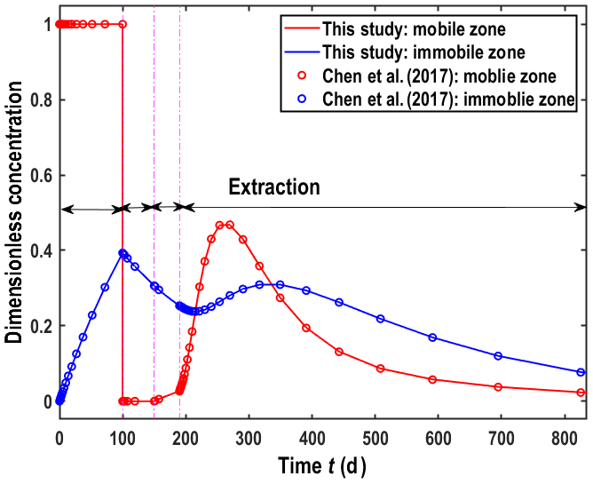
Figure 2Comparison of BTCs at the well screen computed by the solution of this study and Chen et al. (2017).
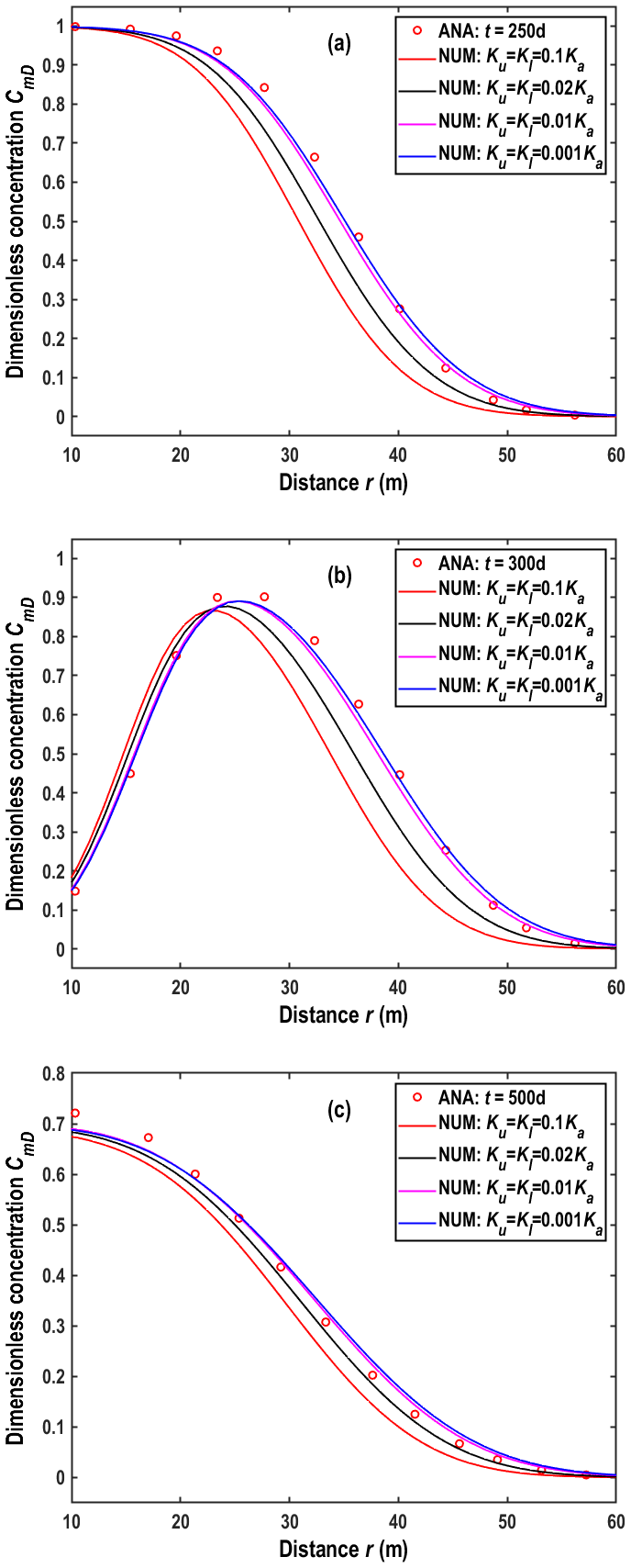
Figure 3Comparison of the concentration distribution between the analytical and numerical solutions along the r axis at z=0 m. “ANA” and “NUM” represent the analytical and numerical solutions, respectively. (a) At the end of the injection phase: t=250 d. (b) At the end of the chasing phase: t=300 d. (c) In the extraction phase: t=500 d.
The water levels in the wellbore in Eqs. (12)–(14) could be calculated by the models of Moench (1985):
where p is Laplace transform variable; L−1 represents the inverse Laplace transform; the over bar represents the Laplace-domain variable, and
where Ku and Kl are hydraulic conductivities (LT−1); Su and Sl are specific storages (L−1); Sw is the wellbore skin factor (dimensionless); Bu and Bl are thicknesses (L); and K0(⋅) and K1(⋅) are the modified Bessel functions.
In this study, the Laplace transform and Green's function methods will be employed to derive the analytical solution of the new SWPP test models described in Sect. 2. The dimensionless parameters are defined as follows: , , , , , , , , , , , , , , , , , , , , , , , and . The detailed derivation of the new solution is listed in Sect. S1 in the Supplement.
3.1 Solutions in the Laplace domain
As for the injection phase of the SWPP test, the solutions in the Laplace domain are
where s represents the Laplace transform parameter for tD (which is proportional to p); Ai(⋅) is the Airy function; is the derivative of the Airy function; and the expressions for a2, b1, E, yinj, yinj, w, εm, εim, εum, εuim, εlm, εlim, βinj and ϕ1 are listed in Table 1.
In the chaser phase, the solutions of the SWPP test in the Laplace domain are
where η varies between rwD and ∞ – e.g., ; ηu varies between 1 and ∞; ηl varies between −1 and −∞; and are the concentrations (ML−3) of the aquifer at the end of injection stage, which could be calculated by Eq. (25a) and (25b) after applying the inverse Laplace transform; and represent the concentrations (ML−3) of the upper aquitard at the end of the injection phase, which could be calculated by Eq. (25c) and (25d) after applying the inverse Laplace transform; and are the concentrations (ML−3) of the lower aquitard at the end of the injection phase, which could be calculated by Eq. (25e) and (25f) after applying the inverse Laplace transform; , and are Green's functions; and the expressions for , , , δ1, δ2, s1, s2, Ea, Eu, El, ycha, ycha, w, F, φ(rD), fu(ηu), X, M1, M2, M3, M4, N1, N2, N3, N4, T1, T2, T3, T4 and βcha, D are listed in Table 2.
For the rest phase, the solutions of the SWPP test in the Laplace domain are
where and are the concentrations (ML−3) of the aquifer at the end of the chaser phase, which could be calculated by Eq. (26a) and (26b) after applying the inverse Laplace transform, and are the concentrations (ML−3) of the upper aquitard at the end of the chaser phase, which could be computed by Eq. (26d) and (26e) after applying the inverse Laplace transform, and and are the concentrations (ML−3) of the lower aquitard at the end of the chaser phase, which could be calculated by Eq. (26f) and (26g) after applying the inverse Laplace transform.
As for the extraction phase of the SWPP test, the solutions in the Laplace domain are
where and are the concentrations (ML−3) of the aquifer at the end of the rest phase, which could be calculated by Eq. (27a) and (27b) after applying the inverse Laplace transform; and are the concentrations (ML−3) of the upper aquitard at the end of the rest phase, which could be calculated by Eq. (27c) and (27d) after applying the inverse Laplace transform; and are the concentrations (ML−3) of the lower aquitard at the end of the rest phase, which could be calculated by Eq. (27e) and (27f) after applying the inverse Laplace transform; bu varies between 1 and ∞; bl varies between −1 and −∞; ε varies between rwD and ∞ (e.g., ; , and are Green's functions; and the expressions for , , , σ1, σ2, Λ, ζ, f(ε), fu(bu), fl(bl), H1∼H4, I1∼I4, m1∼m2, n1∼n2, P1∼P4, W, yext, yext, w and βext, D are listed in Table 3.
Table 1Expressions of the coefficients in the solutions expressed in Eq. (25a)–(25f).

Figure 4The vertical profiles (the r−z profiles) of the concentrations. Panels (a1), (b1) and (c1) represent the analytical solutions at t=250, 300 and 500 d, respectively. Panels (a2), (b2) and (c2) represent the numerical solutions at t=250, 300 and 500 d, respectively.
3.2 Solutions from the Laplace domain to the real-time domain
Because the analytical solutions in the Laplace domain are too complex, it seems impossible to transform it into the real-time domain analytically. Alternatively, a numerical method will be introduced for the inverse Laplace transform. Currently, several methods are available, like the Stehfest model, Zakian model, Fourier series model, de Hoog model and Schapery model (Wang and Zhan, 2015). Here, the de Hoog method will be applied to conduct the inverse Laplace transform, since it performed well for radial-dispersion problems (Wang et al., 2018; Wang and Zhan, 2013).
3.3 Assumptions included in the new SWPP test model
The new SWPP test model is a generalization of several previous studies; for instance, the new solution reduces to the solution of Gelhar and Collins (1971) when , to the solution of Chen et al. (2017) when and that of Wang et al. (2018) when . represents the four-phase SWPP test becoming the two-phase SWPP test, where the chaser and rest phases are excluded. Actually, all values of ωa, ωu, ωl, Du, Dl, vum, vlm, Vw, inj, Vw, cha, and Vw, ext are not zero in reality, which has been considered in the new solutions of this study.
However, three assumptions still remain. First, the flow is in quasi-steady state; e.g., Eq. (15). Second, the groundwater flow is horizontal in the aquifer and is vertical in the aquitard. This treatment relies on the idea that the permeability of the aquitard is smaller than the permeability of the aquifer (Moench, 1985). Third, the model is simplified for the solute transport. For example, only vertical dispersion and advection effects are considered in the aquitard, and only radial dispersion and advection effects are considered in the aquifer. The validation of these assumptions will be discussed in the Sect. 4.2.
In this section, the newly derived analytical solutions will be tested from two aspects. Firstly, the new solution of this study could reduce to previous solutions under special cases, as the model established in this study is an extension of previous ones, and comparisons between them will be shown in Sect. 4.1. Secondly, although some assumptions included in previous models have been relaxed in the new model, some other processes of the reactive transport in the SWPP test have to be simplified in analytical solutions. Assumptions included in the new model have been discussed and their applicability is elaborated in Sect. 4.2.
4.1 Test of the new solution with previous solutions
To test the new solutions, the model of Chen et al. (2017) serves as a benchmark; they ignored the aquitard effect and wellbore storage in the SWPP test. Figure 2 shows the comparison of BTCs between them, and the parameters used in such a comparison are 1, , m, d−1, rw=0.2 m, Qinj=2.5 m3 d−1, Qcha=2.5 m3 d−1, Qres=0 m3 d−1, m3 d−1, tinj=100 d, tcha=50 d, tres=40 d, B=5 m, θm=0.3, θim=0.15, and ω=0.001 d−1. The parameters 0 represent Vw, inj =0, and and imply that wellbore storage is neglected. The values of m d−1 mean that aquitards are neglected. As shown in Fig. 2, both solutions agree well for the mobile and immobile domains.
4.2 Test of assumptions involved in the analytical solution
To test three assumptions outlined in Sect. 3.3, a numerical model will be established, where general three-dimensional transient flow and solute transport are considered in both aquifer and aquitards. A finite-element method with the help of COMSOL Multiphysics will be used to solve the three-dimensional model. The grid system is shown in Sect. S2.
In this study, four sets of aquitard hydraulic conductivities are employed, i.e., , , and . A point to note is that the extreme case of used here is only for the purpose of examining the robustness of comparison, while the real values of Ku and Kl are usually much lower than 0.1 Ka. In other words, the remaining three cases mentioned above are more likely to occur in real applications.
The initial drawdown and the initial concentration are 0 for aquifer and aquitards. The hydraulic parameters are Ka=0.1 m d−1 and m−1, and the other parameters are , , αr=2.5 m, m, s−1, rw=0.5 m, m3 d−1, Qres=0 m3 d−1, m3 d−1, tinj=250 d, tcha=50 d, tres=50 d, B=10 m, θm=0.25, θim=0.05 and ω=0.01 d−1. The comparison of concentration between the analytical and numerical solutions is shown in Figs. 3 and 4.
As the first assumption in Sect. 3.3 has been elaborated on in Sect. S2.2, the following discussion will only focus on the second and third assumptions. Figure 3a, b and c represent the snapshots of concentration distributions in the aquifer along the r axis at different times. One may conclude that curves with smaller Ku and Kl values are closer to the analytical solution. This is because aquitards with smaller Ku and Kl (when Ka remains constant) could make flow closer to the horizontal direction (or parallel with the aquitard–aquifer interface) in the aquifer and closer to the vertical direction (or perpendicular with the aquitard–aquifer interface) in the aquitard, according to the law of refraction (Fetter, 2018). In other words, when the values of Ku∕Ka and Kl∕Ka approach 0, the flow direction becomes horizontal in the aquifer and vertical in the aquitard, and then the numerical model reduces to the analytical model. Therefore, from this figure, one may conclude that the abovementioned second assumption in Sect. 3.3 works well in the aquifer when Ku∕Ka and Kl∕Ka are smaller than 0.01.
Figure 4 shows the comparison of the analytical and numerical solutions for aquitards. Figure 4a1–c1 represent the snapshots of concentration distributions obtained from the analytical solution of this study at different times, and Fig. 4a2–c2 represent the snapshots of concentration distributions obtained from the numerical solution. One may find that the contour maps obtained from both solutions are almost the same in the aquifer, but very different in the aquitards. Therefore, the abovementioned third assumption in Sect. 3.3 is generally unacceptable in describing solute transport in the aquitard in the SWPP test but works well when the aquifer is of primary concern.
5.1 Model applications
As mentioned in Sect.3.3, the new model is a generalization of many previous models, and the conceptual model is closer to reality. However, there are many parameters involved in this new model that have to be determined first for applying this model. For instance, the involved parameters for the aquitards include dispersivity (αu and αl), the first-order mass transfer coefficient (ωu and ωl), the retardation factor (Rum, Ruim, Rlm and Rlim), porosity (θum, θuim, θlm and θlim), reaction rate (μum, μuim, μlm and μlim) and velocity (vum and vlm). The parameters involved for the aquifer include αr, ωa, Rm, Rim, θm, θim and B. Generally, these parameters could not be measured directly. Otherwise, they have to be obtained by fitting the experimental data using the forward model.
Parameter estimation is an inverse problem, and it is generally conducted by an optimization model, such as a genetic algorithm and simulated annealing. Due to the ill-posedness of many inverse problems or insufficient observation data, the initial guess values of unknown parameters of interest are critical for finding the best values or real values of those parameters in the optimization model. Here, we recommend using values of parameters from the literature as the initial guesses for similar lithology. Table 4 lists some parameter values for sandy and clay aquifers in previous studies. When a result is not sensitive to a particular parameter of concern, the value from previous publications for similar lithology and/or situations could be taken as an estimated value of that parameter if there is no direct measurement of that particular parameter of concern. To prioritize the sensitivity of predictions with respect to the diverse parameters involved in the new model, a global sensitivity analysis is conducted in Sect. 5.2.
Table 4A partial list of parameters from the literature.

a Brusseau et al. (1991). b Pickens et al. (1981). c Davis et al. (2003). d Javadi et al. (2017). e Liang et al. (2018). f Swami et al. (2016). g Kookana et al. (1992). h Haggerty et al. (1998). i Bouwer and McCarty (1985). j Chun et al. (2009). k Alvarez et al. (1991). References are shown in Sect. S3.
5.2 A global sensitivity analysis
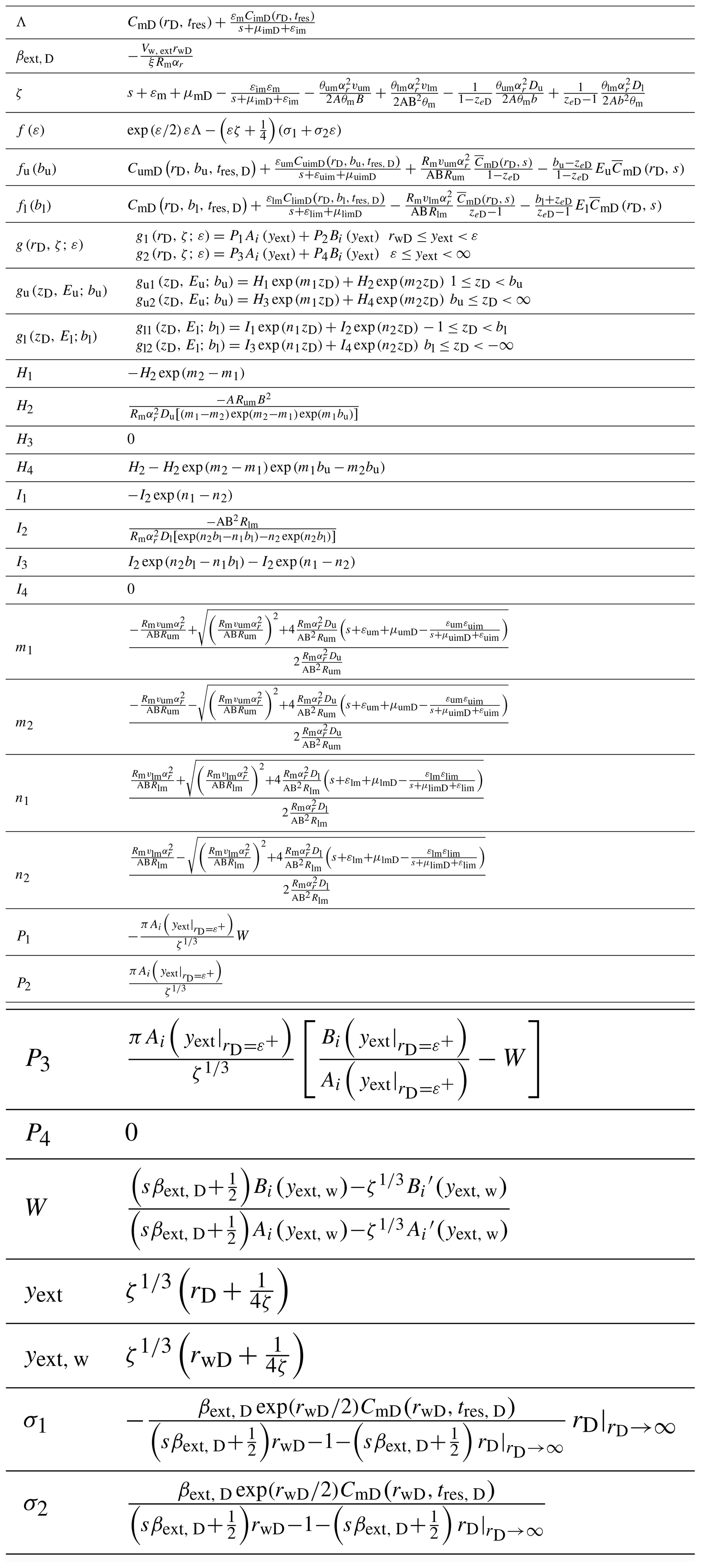
From the analytical solutions of Eqs. (26)–(28), one may find that BTCs are affected by several parameters, like αu, vum, θum, ω, αr, θm and Vw. As αl, vlm and θlm have a similar effect on the results as αu, vum and θum, they have been excluded in the following analysis. In this section, a global sensitivity analysis is conducted using the model of Morris (1991), which is a one-step-at-a-time method. Morris (1991) employed μk and σk to represent the importance of the input parameters for the output concentration, and they have been computed by Morris (1991) and Lin et al. (2019):
where M is the total sampling number, assuming that the range of parameter values is divided by M intervals; N is the total parameter number of interest, and it is 7 in this study; k is the kth parameter. In this study, M=50;
where Pi is the random value of the ith parameter in the range of ; Pi, 0 and Pi, lim are the smallest and largest values of Pi, as shown in Table S1; Δ is a small increment defined as .
A larger μk means a higher sensitive effect of the kth parameter on the output, and a larger σk represents the kth parameter having a greater interaction effect with others. Figure 5a and b represent the variation in μk and σk with time in the wellbore, respectively. The values of μk are greater for αr and θm than for the others, as shown in Fig. 5a, indicating that the influence of θm and αr on the results is more obvious than others. However, the values of σk are large for αu, θum, αr, θm and Vw, demonstrating that the interactions of these parameters with others are strong; namely, the influence of them on results can also not be ignored.
Figure 5Sensitivity analysis. (a) Variation in μk with time in the wellbore. (b) Variation in σk with time in the wellbore.
5.3 Effect of the aquitard
As shown in Sect. 4.2, the new analytical solution is a good approximation for the numerical model in the aquifer when Ku∕Ka and Kl∕Ka are smaller than 0.01. In this section, we try to establish how the aquitards will affect BTCs of the SWPP tests. Since porosity is an important factor of concern, three sets of porosity values are used for the aquitards: , 0.1 and 0.25. The other parameters are from the case in Fig. 4.
Figure 6 shows the difference between the models with and without aquitards for different flow velocities in the aquitard. The case of represents the model without the aquitard. The difference is not obvious at the beginning of the extraction phase, while such a difference is obvious at the late time. Meanwhile, the smaller aquitard porosity makes the value of BTCs in the aquifer greater at a given time. When the aquitard is ignored, the values of BTCs are the greatest. Therefore, the aquitard effect on transport in the aquifer is quite obvious and should not be ignored in general.

Figure 6Comparison of BTCs between the model with and without aquitards for different porosities.
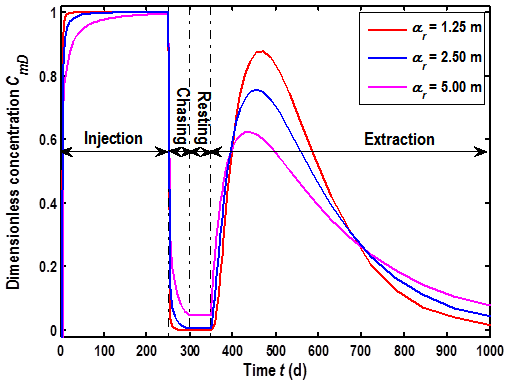
5.4 Effect of the aquifer radial dispersion
Another important parameter is the radial dispersion in the aquifer. In this section, three sets of the radial-dispersivity values will be used to analyze its influence: αr=1.25, 2.50 and 5.00 m.
Figure 7 shows BTCs in the well face for different radial-dispersivity values. Firstly, the difference is obvious among curves in all phases. Secondly, a larger αr could decrease BTCs at a given time of the injection phase. This could be explained by the boundary condition of Eq. (8). The solute in the mobile domain of the aquifer is transported by both advection and dispersion; thus a larger αr could lower the values of Cm in the well face. Thirdly, BTCs increase with increasing αr values in the chaser and rest phases. Fourthly, the peak values of BTCs decrease with increasing αr values.
To test the performance of the new model, the field data reported in Chen et al. (2017) will be employed. Specifically, the experimental data conducted in the borehole TW3 will be analyzed. The reason for choosing this dataset is that this borehole penetrated several layers, and it had been interpreted by Chen et al. (2017) before (using a model that does not consider the aquitard effect and the wellbore storage). The physical parameters of the SWPP test are rw=0.1 m, L min−1, Qres=0 L min−1, Qext=12 L min−1, tinj=180 min, tcha=26.74 min, tres=10 080 min and B=4 m. Other information on the experimental data can be found in Assayag et al. (2009) and Yang et al. (2014).
Figure 8a shows the fitness of the computed and observed BTCs. The estimated parameters are θum=0.05, θlm=0.0, θm=0.1, θim=0.068, αr=0.5 m, αu=0.35 m, αl=0.0 m, , s−1, ω=0.001 d−1, m, m and m. Apparently, the fitness by the new solution is better than the model of Chen et al. (2017). As for the error between the observed and computed BTCs, the new solution is also smaller than that of Chen et al. (2017), where the error is defined as
where COBS and CCOM are the observed and computed concentrations, respectively, and N is the number of sampling points.
How accurate these parameters estimated by best fitting the observed data are in representing the real aquifer will be discussed in the following. The values of the retardation factor and reaction rate demonstrate that the chemical reaction and sorption are weak for the tracer of KBr in the SWPP test. It is not surprising since KBr is commonly treated as a “conservative” tracer. The porosity of the real aquifer ranges from 0.01 to 0.1, according to the well log analysis (Yang et al., 2014), where the estimated values are located. The estimated porosity represents the average values of the aquifer and aquitards. The estimated dispersivity of the aquifer is 0.7134 m by Chen et al. (2017), which is similar to ours. The values of the water level in the test could be observed directly; however, these data are not available, and they have to be estimated in this study. To evaluate the uncertainty in the estimated parameters, the sensitivity of the dispersivity to BTCs is analyzed, as shown in Fig. 8b. One may conclude that the estimated values of this study seem to be representative of reality, since the error is smallest for αr=0.5 m.
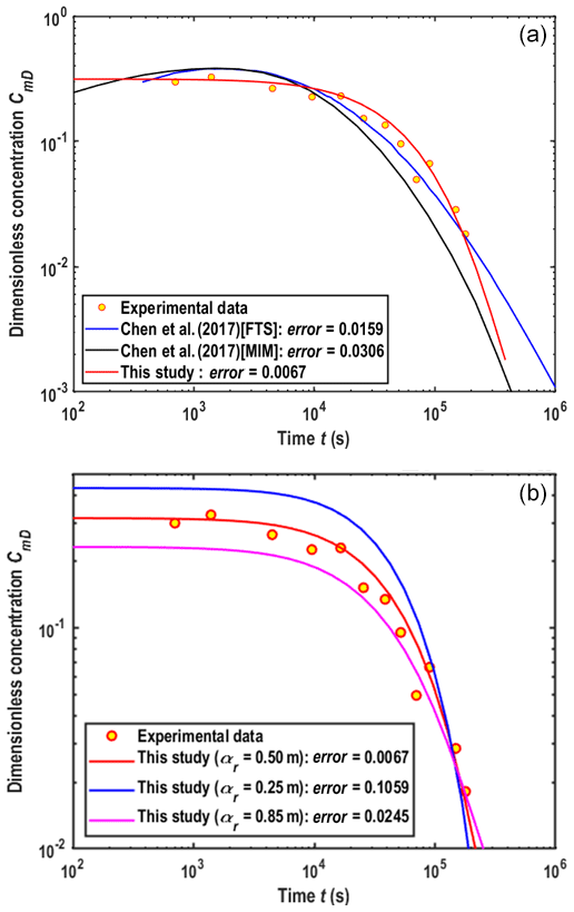
Figure 8Fitness of observed BTC. (a) Fitness of the observed data by different models. (b) Influence of the dispersivity of the aquifer on BTCs.
The single-well push–pull (SWPP) test could be applied to estimate the dispersivity, porosity and chemical reaction rates of in situ aquifers. However, previous studies mainly focused on an isolated aquifer, excluding all the possible effects of aquitards bounding the aquifer. In other words, the adjacent layers are assumed to be non-permeable, which is not exactly true in reality. In this study, a new analytical model is established and its associate solutions are derived to inspect the effect of overlying and underlying aquitards. Meanwhile, four stages are considered in the new model with wellbore storage: the injection phase, the chaser phase, the rest phase and the extraction phase. The anomalous behaviors of reactive transport in the test were described by a mobile–immobile framework.
To derive the analytical solution of the new model, some assumptions are inevitable. For instance, only vertical advection and dispersion are considered in the aquitard and only horizontal advection and dispersion are considered in the aquifer, and the flow is quasi-steady state. Although these assumptions have been widely used to describe the radial dispersion in previous studies, the influences on reactive transport have not been discussed in a rigorous sense before. In this study, numerical modeling exercises are introduced to test the abovementioned assumptions of the new model. Based on this study, several conclusions could be obtained.
-
A new model of the SWPP test is a generalization of many previous models by considering the aquitard effect, the wellbore storage and the mass transfer rate in both aquifer and aquitards. A sub-model of wellbore storage is developed.
-
The assumption of vertical advection and dispersion in the aquitard and horizontal advection and dispersion in the aquifer are tested by specially designed finite-element numerical models using COMSOL, and the result shows that this assumption is acceptable when the aquifer is of primary concern, provided that the ratios of the aquitard or aquifer permeability are less than 0.01, while such an assumption is generally unacceptable when the aquitards are of concern, regardless of the ratios of the aquitard or aquifer permeability.
-
The new model is more sensitive to αr and θm after a global sensitivity analysis, and the values of σk are large for αu, θum, αr, θm and Vw, demonstrating that the influence of the aquitard on results could not be ignored.
-
The performance of the new model is better than previous models that exclude the aquitard effect and the wellbore storage in terms of best fitting exercises with field data reported in Chen et al. (2017).
All data are available in the Supplement.
The supplement related to this article is available online at: https://doi.org/10.5194/hess-24-3983-2020-supplement.
QW wrote the paper and developed the mathematic models; JW and WS derived the analytical solutions; HZ revised the paper.
The authors declare that they have no conflict of interest.
We thank the editor, associate editor and two anonymous reviewers for their constructive comments, which helped improve the quality of the paper.
The authors declare that they have no conflict of interest.
This research was partially supported by programs of the Natural Science Foundation of China (grant nos. 41772252, 41972250 and 41502229), Innovative Research Groups of the National Nature Science Foundation of China (grant no. 41521001), the Natural Science Foundation of Hubei Province, China (grant no. 2018CFA028), the Fundamental Research Funds for the Central Universities, China University of Geosciences (Wuhan) (grant no. CUGGC07) and China Geological Survey (grant nos. DD20190263, 2019040022).
This paper was edited by Philippe Ackerer and reviewed by two anonymous referees.
Alvarez, P. J. J., Anid, P. J., and Vogel, T. M.: Kinetics of aerobic biodegradation of benzene and toluene in sandy aquifer material, Biodegradation, 2, 43–51, https://doi.org/10.1007/bf00122424, 1991.
Assayag, N., Matter, J., Ader, M., Goldberg, D., and Agrinier, P.: Water-rock interactions during a CO2 injection field-test: Implications on host rock dissolution and alteration effects, Chem. Geol., 265, 227–235, https://doi.org/10.1016/j.chemgeo.2009.02.007, 2009.
Bouwer, E. J. and McCarty, P. L.: Utilization rates of trace halogenated organic compounds in acetate-grown biofilms, Biotechnol. Bioeng., 27, 1564–1571, https://doi.org/10.1002/bit.260271107, 1985.
Brusseau, M. L., Jessup, R. E., and Rao, P. S. C.: Nonequilibrium sorption of organic chemicals: elucidation of rate-limiting processes, Environ. Sci. Technol., 25, 134–142, https://doi.org/10.1021/es00013a0151991, 1991.
Chen, C. S.: Analytical and approximate solutions to radial dispersion from an injection well to a geological unit with simultaneous diffusion into adjacent strata, Water Resour. Res., 21, 1069–1076, https://doi.org/10.1029/WR021i008p01069, 1985.
Chen, C. S.: Analytical solutions for radial dispersion with Cauchy boundary at injection well, Water Resour. Res., 23, 1217–1224, https://doi.org/10.1029/WR023i007p01217, 1987.
Chen, J. S., Chen, C. S., and Chen, C. Y.: Analysis of solute transport in a divergent flow tracer test with scale-dependent dispersion, Hydrol. Process., 21, 2526–2536, https://doi.org/10.1002/hyp.6496, 2007.
Chen, K., Zhan, H., and Yang, Q.: Fractional models simulating non-fickian behavior in four-stage single-well injection-withdrawal tests, Water Resour. Res., 53, 9528–9545, https://doi.org/10.1002/2017WR021411, 2017.
Chen, Y. J., Yeh, H. D., and Chang, K. J.: A mathematical solution and analysis of contaminant transport in a radial two-zone confined aquifer, J. Contam. Hydrol., 138, 75–82, https://doi.org/10.1016/j.jconhyd.2012.06.006, 2012.
Chowdhury, A. I. A., Gerhard, J. I., Reynolds, D., Sleep, B. E., and O'Carroll, D. M.: Electrokinetic-enhanced permanganate delivery and remediation of contaminated low permeability porous media, Water Res., 113, 215–222, https://doi.org/10.1016/j.watres.2017.02.005, 2017.
Chun, J. A., Cooke, R. A., Eheart, J. W., and Kang, M. S.: Estimation of flow and transport parameters for woodchip-based bioreactors: I. laboratory-scale bioreactor, Biosyst. Eng., 104, 384395, https://doi.org/10.1016/j.biosystemseng.2009.06.021, 2009.
Davis, B. M., Istok, J. D., and Semprini, L.: Static and push–pull methods using radon-222 to characterize dense non aqueous phase liquid saturations, Groundwater, 41, 470–481, https://doi.org/10.1111/j.1745-6584.2003.tb02381.x, 2003.
Fetter, C. W.: Applied hydrogeology, Prentice-Hall, Inc, 589 pp., ISBN 9780130882394, 0130882399, 2018.
Gelhar, L. W. and Collins, M. A.: General analysis of longitudinal dispersion in nonuniform flow, Water Resour. Res., 7, 1511–1521, https://doi.org/10.1029/WR007i006p01511, 1971.
Guarracino, L., Carrera, J., and Vázquez-Suñé, E.: Analytical study of hydraulic and mechanical effects on tide-induced head fluctuation in a coastal aquifer system that extends under the sea, J. Hydrol., 450, 150–158, https://doi.org/10.1016/j.jhydrol.2012.05.015 2012.
Haggerty, R. and Gorelick, S. M.: Multiple-rate mass-transfer for modeling diffusion and surface-reactions in media with pore-scale heterogeneity, Water Resour. Res., 31, 2383–2400, https://doi.org/10.1029/95WR10583, 1995.
Haggerty, R., Schroth, M. H., and Istok, J. D.: Simplified Method of “Push-Pull” Test Data Analysis for Determining In Situ Reaction Rate Coefficients, Groundwater, 36, 314–324, https://doi.org/10.1111/j.1745-6584.1998.tb01097.x, 1998.
Haggerty, R., McKenna, S. A., and Meigs, L. C.: On the late-time behavior of tracer test breakthrough curves, Water Resour. Res., 36, 3467–3479, https://doi.org/10.1029/2000wr900214, 2000.
Hansen, S. K., Vesselinov, V. V., Reimus, P. W., and Lu, Z.: Inferring subsurface heterogeneity from push-drift tracer tests, Water Resour. Res., 53, 6322–6329, https://doi.org/10.1002/2017WR020852, 2017.
Hantush, M. S.: Flow of groundwater in relatively thick leaky aquifers, Water Resour. Res., 3, 583–590, https://doi.org/10.1029/WR003i002p00583, 1967.
Huang, J. Q., Christ, J. A., and Goltz, M. N.: Analytical solutions for efficient interpretation of single-well injection-withdrawal tracer tests, Water Resour. Res., 46, W08538, https://doi.org/10.1029/2008wr007647, 2010.
Javadi, S., Ghavami, M., Zhao, Q., and Bate, B.: Advection and retardation of non polar contaminants in compacted clay barrier material with organoclay amendment, Appl. Clay Sci., 142, 30–39, https://doi.org/10.1016/j.clay.2016.10.041, 2017.
Jung, Y. and Pruess, K.: A closed-form analytical solution for thermal single-well injection-withdrawal tests, Water Resour. Res., 48, W03504, https://doi.org/10.1029/2011WR010979, 2012.
Kabala, Z. J.: Sensitivity analysis of a pumping test on a well with wellbore storage and skin, Adv. Water Resour., 24, 483–504, https://doi.org/10.1016/s0309-1708(00)00051-8, 2001.
Kookana, R. S., Aylmore, L. A. G., and Gerritse, R. G.: Time-dependent sorption of pesticides during transport in soils, Soil Science, 154, 214–225, https://doi.org/10.1097/00010694-199209000-00005, 1992.
Li, Z. F., Zhou, Z. F., Dai, Y. F., and Dai, B. B.: Contaminant transport in a largely-deformed aquitard affected by delayed drainage, J. Contam. Hydrol., 221, 118–126, https://doi.org/10.1016/j.jconhyd.2019.02.002, 2019.
Liang, X., Zhan, H., Liu, J., Dong, G., and Zhang, Y.: A simple method of transport parameter estimation for slug injecting tracer tests in porous media, Sci. Total Environ., 644, 1536–1546, https://doi.org/10.1016/j.scitotenv.2018.06.330, 2018.
Lin, Y. C., Hu, T. F., and Yeh, H. D.: Analytical model for heat transfer accounting for both conduction and dispersion in aquifers with a Robin-type boundary condition at the injection well, Water Resour. Res., 55, 7379–7399, https://doi.org/10.1029/2019WR024966, 2019.
Moench, A. F.: Transient flow to a large-diameter well in an aquifer with storative semiconfining layers, Water Resour. Res., 21, 1121–1131, https://doi.org/10.1029/WR021i008p01121, 1985.
Moench, A. F.: Convergent radial dispersion: A Laplace transform solution for aquifer tracer testing, Water Resour. Res., 25, 439–447, https://doi.org/10.1029/WR025i003p00439, 1989.
Morris, M. D.: Factorial sampling plans for preliminary computational experiments, Technometrics, 33, 161–174, https://doi.org/10.1080/00401706.1991.10484804, 1991.
Phanikumar, M. S. and McGuire, J. T.: A multi-species reactive transport model to estimate biogeochemical rates based on single-well injection-withdrawal test data, Comput. Geosci., 36, 997–1004, https://doi.org/10.1016/j.cageo.2010.04.001, 2010.
Pickens, R., Jackson, K., and Meritt, W.: Measurement of distribution coeffcients using a radial injection dual-tracer test, Water Resour. Res., 17, 529–544, https://doi.org/10.1029/WR017i003p00529, 1981.
Schroth, M. H., Istok, J. D., and Haggerty, R.: In situ evaluation of solute retardation using single-well injection-withdrawal tests, Adv. Water Resour., 24, 105–117, https://doi.org/10.1016/S0309-1708(00)00023-3, 2001.
Schroth, M. H. and Istok, J. D.: Approximate solution for solute transport during spherical-flow push-pull tests, Groundwater, 43, 280–284, https://doi.org/10.1111/j.1745-6584.2005.0002.x, 2005.
Sudicky, E. A.: A natural gradient experiment on solute transport in a sand aquifer: Spatial variability of hydraulic conductivity and its role in the dispersion process, Water Resour. Res., 24, 1211–1216, https://doi.org/10.1029/WR024i007p01211, 1988.
Swami, D., Sharma, P. K., and Ojha, C. S. P.: Behavioral Study of the Mass Transfer Coefficient of Nonreactive Solute with Velocity, Distance, and Dispersion, J. Environ. Eng., 143, 04016076, https://doi.org/10.1061/(asce)ee.1943-7870.0001164, 2016.
Tang, D. H. and Babu, D. K.: Analytical solution of a velocity dependent dispersion problem, Water Resour. Res., 15, 1471–1478, https://doi.org/10.1029/WR015i006p01471, 1979.
Wang, Q. R. and Zhan, H. B.: Radial reactive solute transport in an aquifer-aquitard system, Adv. Water Resour., 61, 51–61, https://doi.org/10.1016/j.advwatres.2013.08.013, 2013.
Wang, Q. R. and Zhan, H. B.: On different numerical inverse Laplace methods for solute transport problems, Adv. Water Resour., 75, 80–92, https://doi.org/10.1016/j.advwatres.2014.11.001, 2015.
Wang, Q. and Zhan, H.: Reactive transport with wellbore storages in a single-well push–pull test, Hydrol. Earth Syst. Sci., 23, 2207–2223, https://doi.org/10.5194/hess-23-2207-2019, 2019.
Wang, Q. R., Shi, W., Zhan, H., Gu, H., and Chen, K.: Models of single-well injection-withdrawal test with mixing effect in the wellbore, Water Resour. Res., 54, 10155–10171, https://doi.org/10.1029/2018WR023317, 2018.
Yang, Q., Matter, J., Stute, M., Takahashi, T., O'Mullan, G., Umemoto, K., Clauson, K., Dueker, M. E., Zakharova, N., Goddard, J., and Goldberg, D.: Groundwater hydrogeochemistry in injection experiments simulating CO2 leakage from geological storage reservoir, Int. J. Greenh. Gas Control, 26, 193–203, https://doi.org/10.1016/j.ijggc.2014.04.025, 2014.
Zhan, H. B., Wen, Z., and Gao, G. Y.: An analytical solution of two-dimensional reactive solute transport in an aquifer-aquitard system, Water Resour. Res., 45, W10501, https://doi.org/10.1029/2008wr007479, 2009.
Zhou, R., Zhan, H., and Chen, K.: Reactive solute transport in a filled single fracture-matrix system under unilateral and radial flows, Adv. Water Resour., 104, 183–194, https://doi.org/10.1016/j.advwatres.2017.03.022, 2017.
Zlotnik, V. A. and Zhan, H. B.: Aquitard effect on drawdown in water table aquifers, Water Resour. Res., 41, W06022, https://doi.org/10.1029/2004wr003716, 2005.
- Abstract
- Introduction
- Model statement of the SWPP test
- New solution of reactive transport in the SWPP test
- Verification of the new model
- Discussions
- Data interpretation: field SWPP test
- Summary and conclusions
- Data availability
- Author contributions
- Competing interests
- Acknowledgements
- Competing interests
- Financial support
- Review statement
- References
- Supplement