the Creative Commons Attribution 4.0 License.
the Creative Commons Attribution 4.0 License.
 | 07 Aug 2020
Revisiting the global hydrological cycle: is it intensifying?
As a result of technological advances in monitoring atmosphere, hydrosphere, cryosphere and biosphere, as well as in data management and processing, several databases have become freely available. These can be exploited in revisiting the global hydrological cycle with the aim, on the one hand, to better quantify it and, on the other hand, to test the established climatological hypotheses according to which the hydrological cycle should be intensifying because of global warming. By processing the information from gridded ground observations, satellite data and reanalyses, it turns out that the established hypotheses are not confirmed. Instead of monotonic trends, there appear fluctuations from intensification to deintensification, and vice versa, with deintensification prevailing in the 21st century. The water balance on land and in the sea appears to be lower than the standard figures of literature, but with greater variability on climatic timescales, which is in accordance with Hurst–Kolmogorov stochastic dynamics. The most obvious anthropogenic signal in the hydrological cycle appears to be the over-exploitation of groundwater, which has a visible effect on the rise in sea level. Melting of glaciers has an equal effect, but in this case it is not known which part is anthropogenic, as studies on polar regions attribute mass loss mostly to ice dynamics.
Please read the editorial note first before continuing.
-
Please read the editorial note first before accessing the article.
-
Article
(16327 KB)
-
Please read the editorial note first before accessing the article.
- Article
(16327 KB) - Full-text XML
- Editorial note
- BibTeX
- EndNote


If the dark side of concerns about Earth's climate is fear, the bright side is data. The latter single-word label means to include the technological advances in monitoring atmosphere, hydrosphere, cryosphere and biosphere, the gathering and processing of huge amounts of ground- and space-based observations for the land and sea parts of the Earth, and the free availability of data. Hydrological processes on the global scale extend over all these spheres, and our knowledge of them benefits from these data.
The availability of different types of data allows revisiting the global hydrological cycle and improving its quantified knowledge. It can also be useful in testing the climatological hypotheses that are relevant to hydrology. Among them, most crucial is the conjecture that, in a warming climate, atmospheric moisture is changing in a manner in which the relative humidity remains constant but specific humidity increases, according to the Clausius–Clapeyron relationship. As a result, the established view is that the global atmospheric water vapour should increase by about 6 %–7 % ∘C−1 of warming. This gives rise to what has been called the intensification of the hydrological cycle. Because of the alleged intensification, the role of hydrology becomes thus important in the climate agenda from a sociological point of view; some of the most prominent predicted catastrophes are related to water shortage and extreme floods (Koutsoyiannis, 2014a).
Hence, the purpose of this study is to revisit the hydrological cycle in an era of climate change concerns and rich data availability, with an emphasis on the following points:
-
providing an overview of and retrieving a great number of global hydroclimatic data sets;
-
improving the quantification of the global hydrological cycle, its variability and its uncertainties through the surge of newly available data sets;
-
testing established climatological hypotheses according to which the hydrological cycle should be intensifying because of global warming;
-
outlining a stochastic view of hydroclimate which provides reliable means to deal with its variability.
These points are reflected in the structure of the paper in the following manner. The material related to point 1 is detailed in Sect. 2. Sections 3–5 are aligned according to point 2, namely the quantification of the global hydrological cycle. On the other hand, point 3 elevates the significance of atmospheric water and, thus, Sect. 3 is devoted to this topic. Precipitation and evaporation are the key components of the hydrological cycle, as their imbalance in the land part of Earth drives all other hydrological processes. Quantification and changes in these drivers are examined in Sect. 4. Based on the results in Sect. 4, the water balance per se is studied in Sect. 5. Moreover, to quantify storage changes within water balance, and in particular the groundwater and cryosphere storage changes, Sect. 5 includes an extended review of related literature.
Point 3 is dealt with, together with point 2, in Sects. 3 and 4, which is devoted to the atmospheric water, precipitation and evaporation, and in two Appendices, which provide additional information on testing established climatological hypotheses. Point 4 is contained in Sect. 6, in which the scope is the future hydroclimatic variability. The necessity of proposing a stochastic approach to hydroclimate becomes obvious after examining whether climate models (and other more empirical techniques commonly used) are consistent with the reality (tracked in the earlier sections) and skilful, so as to be usable for future hydrological projections. It turns out that the state of affairs with current common methodologies is not satisfactory, and hence the need for an alternative approach emerges. This has to be stochastic and consistent with observed natural behaviours, as outlined in Sect. 6. Finally, Sect. 7 concludes the study with relevant remarks.
2.1 Sources of information
This study tries to use a wide range of available data sets reflecting the real-world hydrological cycle at the global level, either directly (by accessing the data per se) or indirectly (by using processed data and results from other studies). In particular, the information used comprises the following: (a) gridded ground observations, (b) satellite data and (c) reanalysis data. Gridded ground observations are available for precipitation over land. Gridded satellite data exist for several variables of hydrologic importance, including air temperature, water vapour amount, cloud water amount, precipitation and snow cover, as detailed in the next subsections. Information from reanalyses is far richer, as this provides a numerical description of the weather system, in terms of a great deal of atmospheric variables, by combining numerical weather prediction models with observations. Here we use the Reanalysis 1 by the National Centers for Environmental Prediction (NCEP) and the National Center for Atmospheric Research (NCAR), collectively NCEP–NCAR, and the ERA5 reanalysis, which are publicly available.
The temporal coverage of the NCEP–NCAR Reanalysis 1 (Kalnay et al., 1996) includes data collected four times daily to provide daily and monthly values from 1948 to the present at a horizontal resolution of 1.88∘ (∼210 km). It uses a state-of-the-art analysis and forecast system to perform data assimilation, using observations and a numerical weather prediction model. The data assimilation and the model used are identical to the global system implemented operationally at NCEP, except in the horizontal resolution. A large subset of the data is available as daily and monthly averages.
The ERA5 (Copernicus Climate Change Service, 2017) is the fifth-generation atmospheric reanalysis of the European Centre for Medium-Range Weather Forecasts (ECMWF), where the name ERA refers to ECMWF reanalysis. It spans the modern observational period, from 1979 onwards, with daily updates continuing forward in time, and fields available at a horizontal resolution of 31 km on 139 levels from the surface up to 0.01 hPa (around 80 km). It has been produced as an operational service, and its fields compare well with the ECMWF operational analyses (Hersbach and Dee, 2016).
We did not use the longer-term reanalyses that appeared recently to serve climate change studies, as these have lower reliability. Specifically, the ERA-20C reanalysis, which covers the period 1900–2010, compares poorly even to the ERA5 reanalysis, developed by the same institution (ECMWF), while the 20th century reanalysis V3 (20CR V3 by the National Oceanic and Atmospheric Association (NOAA), the Cooperative Institute for Research in Environmental Sciences (CIRES) and the Department of Energy (DOE), collectively NOAA–CIRES–DOE), which covers the period 1836–2015 has, in addition, huge departures of the precipitation from the evaporation quantities over the globe, with the global imbalance being more than half of the precipitation over land or almost twice the runoff. Therefore, here they are judged as not hydrologically useful.
In addition, this study uses results from several other studies which are based on different data sets, such as the Gravity Recovery and Climate Experiment (GRACE; Syed et al., 2009; Eicker et al., 2016; Schellekens et al., 2017); NASA's Global Land Data Assimilation System (GLDAS; Zhou et al., 2019); and hydrological models such as the global gridded monthly reconstruction of runoff (GRUN; 1902–2014; Ghiggi et al., 2019) or the PCRaster Global Water Balance (PCR-GLOBWB; Wada et al., 2010). Archfield et al. (2015) provide additional links to other useful data sources.
In the next subsections we describe each data set used, while in Table 1 we summarize all the details and provide all necessary links to the retrieved information so that the reader can easily reproduce the results of this study. In general, we use actual values of time series, disfavouring the popular notion of “anomalies”, i.e. for differences from a certain mean1, which have only a statistical, rather than a physical, meaning while, even in a statistical context, they have several disadvantages (e.g. they hide biases). Thus, whenever possible, data originally given as “anomalies” are converted here to actual values. As the “anomalies” are usually taken from monthly means, by converting them to actual values we reinstate the seasonality. For this reason, the information given in this study in terms of graphs differs substantially from familiar graphs of the climatic literature. This is a deliberate choice in an attempt not to hide the variability. All graphs also include running averages on the annual scale, and thus the temporal mean and variability on annual and multi-year scales are also highlighted in the graphs.
Table 1List and details of variables and data sets used in the study (unless otherwise stated in a particular entry, all data were last accessed in February 2020).
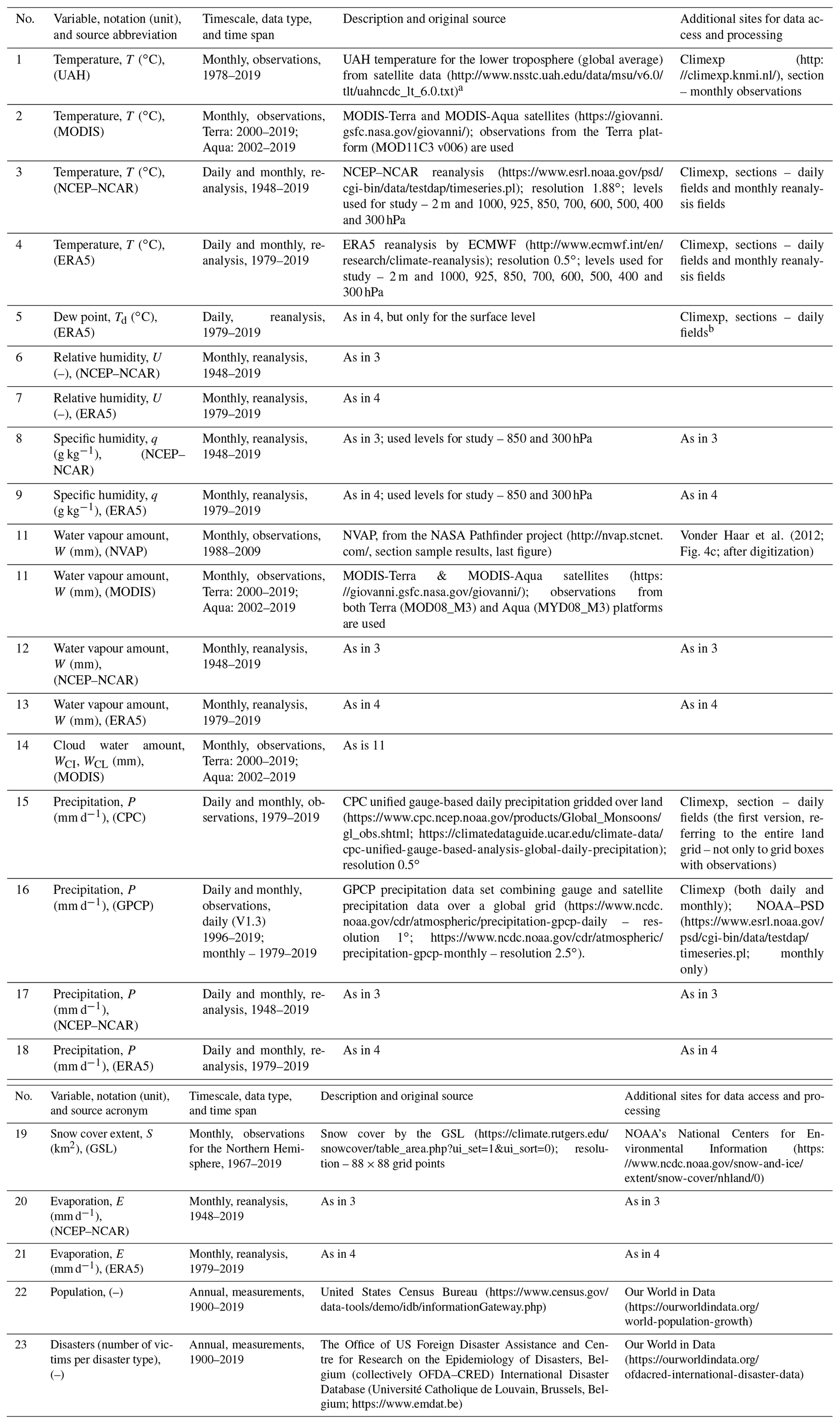
a The data set is given as the “anomalies”. To convert the “anomalies” to actual temperatures we used the monthly averages, which are available at:
http://www.drroyspencer.com/2016/03/uah-v6-lt-global-temperatures-with-annual-cycle/.
b For the NCEP–NCAR daily and monthly reanalysis neither the dew
point nor the relative humidity at the surface level is available.
2.2 Temperature and dew point data
The satellite temperature data set, developed at the University of Alabama in Huntsville (UAH), infers the temperature, T, of three broad levels of the atmosphere from satellite measurements of the oxygen radiance in the microwave band, using advanced (passive) microwave sounding units on NOAA and NASA satellites (Spencer and Christy, 1990; Christy et al., 2007). The data are publicly available on a monthly scale in the form of time series of “anomalies” for several parts of the Earth and in maps. Here we use only the global average on a monthly scale for the lowest level, referred to as the lower troposphere, after the conversion of the “anomalies” to actual temperatures.
For the more recent years, monthly land surface temperature and emissivity are also available from the Moderate Resolution Imaging Spectroradiometer (MODIS), a key instrument aboard two satellites, namely the Terra (originally known as EOS AM-1) and the Aqua (originally known as EOS PM-1), providing observations since 2000 and 2002, respectively. The MOD11C3 Version 6 product provides temperature values on a 0.05∘ grid, which are derived by compositing and averaging the values from the corresponding month of MOD11C1 daily files (Wan, 2013; Wan et al., 2015). Here the Terra data set has been retrieved, and the average monthly temperature over land has been derived by averaging the daytime and nighttime data sets.
The NCEP–NCAR and ERA5 reanalyses provide more detailed information for T at the daily and monthly timescale, not only near the surface (2 m above ground) but also at several atmospheric levels, of which those of 1000, 925, 850, 700, 600, 500, 400 and 300 hPa are used in the study.
For the same levels, data for relative humidity, U, are also provided at the monthly scale; from the temperature and relative humidity, the dew point, Td, can be estimated (Eq. 4 below). In addition, the ERA5 daily reanalysis provides, independently, the daily dew point for the surface level.
2.3 Atmospheric water data
As already mentioned, the relative humidity, U, is available at the monthly scale at several atmospheric levels for both reanalyses. In addition, the specific humidity, q (see Eq. 5 below), is independently available and was retrieved at the levels of 850 and 300 hPa. The reanalyses fields also include data for the water vapour amount, W (also known as “vertically integrated water vapour”, or “precipitable water”2 and expressed in mm or equivalently kg m−2).
In addition, W is provided from satellite observations in two data sets, namely the NASA Water Vapor Project (NVAP) and MODIS. The NVAP data set is a model-independent data set relying mainly on satellite measurements from the NASA Pathfinder project (Vonder Haar et al., 2012). The monthly data for the period 1988–2009 over the globe are available in the form of a graph, which has been digitized here. For the more recent years, W is also available from the MODIS satellites Terra and Aqua mentioned above (Platnick et al., 2015; Hubanks et al., 2015). In addition, the MODIS platforms provide data for the column amount of ice (WCI) and liquid water (WCL) in the clouds, also known as the “cloud ice water path” and “cloud liquid water path”, respectively; these are also used in the study.
2.4 Precipitation data
Gridded ground data for precipitation rate, P (mm d−1), over land are available from the Climate Prediction Center's (CPC) unified gauge-based analysis of global daily precipitation for the period from 1979 to the present. This is based on gauge reports from over 30 000 stations, collected from multiple sources, including national and international agencies. Quality control is performed through comparisons with historical records and independent information from measurements at nearby stations, concurrent radar and satellite observations, as well as numerical model forecasts. Quality-controlled station reports are then interpolated to create analysed fields of daily precipitation with the consideration of orographic effects (Xie et al., 2007). The daily analysis is constructed on a 0.125∘ grid over the entire global land area and is released on a 0.5∘ grid (Xie, 2010). This data set has two components, namely the “retrospective version”, which uses 30 000 stations and spans 1979–2005, and the “real-time version”, which uses 17 000 stations and spans 2006–present; the latter data set has been planned to be reprocessed for consistency with the retrospective analysis. Here all data are used for both the daily and monthly scale.
Another gridded precipitation data set, this time also extending over the sea, is the data set of the Global Precipitation Climatology Project (GPCP), which combines gauge and satellite precipitation data over a global grid. The general approach is to combine the precipitation information available from each of several satellites and in situ sources into a final merged product, taking advantage of the strengths of each data type. Passive microwave estimates are based on Special Sensor Microwave Imager/Special Sensor Microwave Imager Sounder (SSMI–SSMIS) data; infrared precipitation estimates are included using Geostationary Operational Environmental Satellite (GOES) data and Polar-orbiting Operational Environmental Satellite (POES) data and other low Earth-orbit data and in situ observations (Adler et al., 2016). Monthly data are provided on a 2.5∘ grid and are available for the period from 1979 to the present. The GPCP daily analysis is a companion to the monthly analysis, and it provides globally complete precipitation estimates at a spatial resolution of 1∘ and daily timescale from October 1996 to the present. Although derived using both some of the same, but also some different, data sets and methods compared to those used in the GPCP monthly analysis, the daily data add up to the monthly data (Huffman et al., 2001; Adler et al., 2017).
The NCEP–NCAR and ERA5 reanalyses also provide gridded daily and monthly precipitation data.
Information about snow is provided by satellite data. The most complete data set of this type is the snow cover extent for the Northern Hemisphere (NH), monitored via satellites by the US National Oceanic and Atmospheric Administration (NOAA) from 1966 to the present, updated monthly. Data prior to June 1999 are based on satellite-derived maps of the NH snow cover extent produced weekly by trained NOAA meteorologists; after that date, they have been produced by daily output from the Interactive Multisensor Snow and Ice Mapping System (IMS). The data are provided on a Cartesian grid with 88×88 cells laid over a NH polar stereographic projection, where each grid cell has a binary value indicating whether it has snow cover or is snow free (see details in Robinson et al., 2012, and Estilow et al., 2015). The snow cover extent in the Southern Hemisphere is not currently monitored.
2.5 Evaporation data
At present, the evaporation rate, E (mm d−1), cannot be measured at large scales and is estimated only by models. Here the monthly data sets by the NCEP–NCAR and ERA5 reanalyses are used.
2.6 Data access and processing systems
There are lots of software applications to analyse and process gridded data. Here we are using free web platforms that are easy to use and allow direct reproducibility of the results by the interested reader; the links to these platforms are given in Table 1.
Most of the processing in this study has been made via the Climate Explorer (Climexp) system of the Royal Netherlands Meteorological Institute (Koninklijk Nederlands Meteorologisch Instituut – KNMI). This very powerful system combines access to many sources of data, including most of the data sets used here, but also data from individual stations and multiple processing options. The data access includes, among other options, daily fields of observations and reanalyses, monthly observations and monthly reanalysis fields. The processing options include averaging over geographical areas (including prespecified or user-defined “masks”, i.e. polygons defined by a set of connected (x, y) points), aggregating at larger scales, computing zonal means, making time series, and calculating their statistics and plotting the fields.
NASA's Giovanni online web environment is another useful tool for the access, display and analysis of NASA's geophysical data (Acker and Leptoukh, 2007). A similar system for NOAA's data, which also incorporates data for fields of additional sources, is the Web-based Reanalyses Intercomparison Tools (WRITs; Earth System Research Laboratory's Physical Sciences Division; see Smith et al., 2014).
Access to some of the data which are not contained in the above three systems is provided by other platforms, as specified in Table 1.
3.1 Atmospheric temperature and dew point
For the study of atmospheric water, air temperature is an important variable and thus we start with this. Figure 1a shows the evolution of global average temperature at the level of 2 m above ground at the monthly and annual scale, according to both reanalyses data, NCEP–NCAR and ERA5. In addition, Fig. 1b depicts satellite data in comparison to reanalysis ones but at a higher altitude. Specifically, the UAH satellite time series is used, which refers to the lower troposphere. Comparing this to reanalysis data at several pressure levels, we found that it roughly corresponds to the weighted averages of those at the levels of 500 and 700 hPa, with weights of 0.62 and 0.38, respectively. Figure 1 shows a good agreement of all three information sources at both pressure levels. At the same time, they show a gradual increase in temperature, with about the same rate of increase. All three sources provide complete information for the last 40 years, while one of them, NCEP–NCAR, has a longer span, namely 68 years.
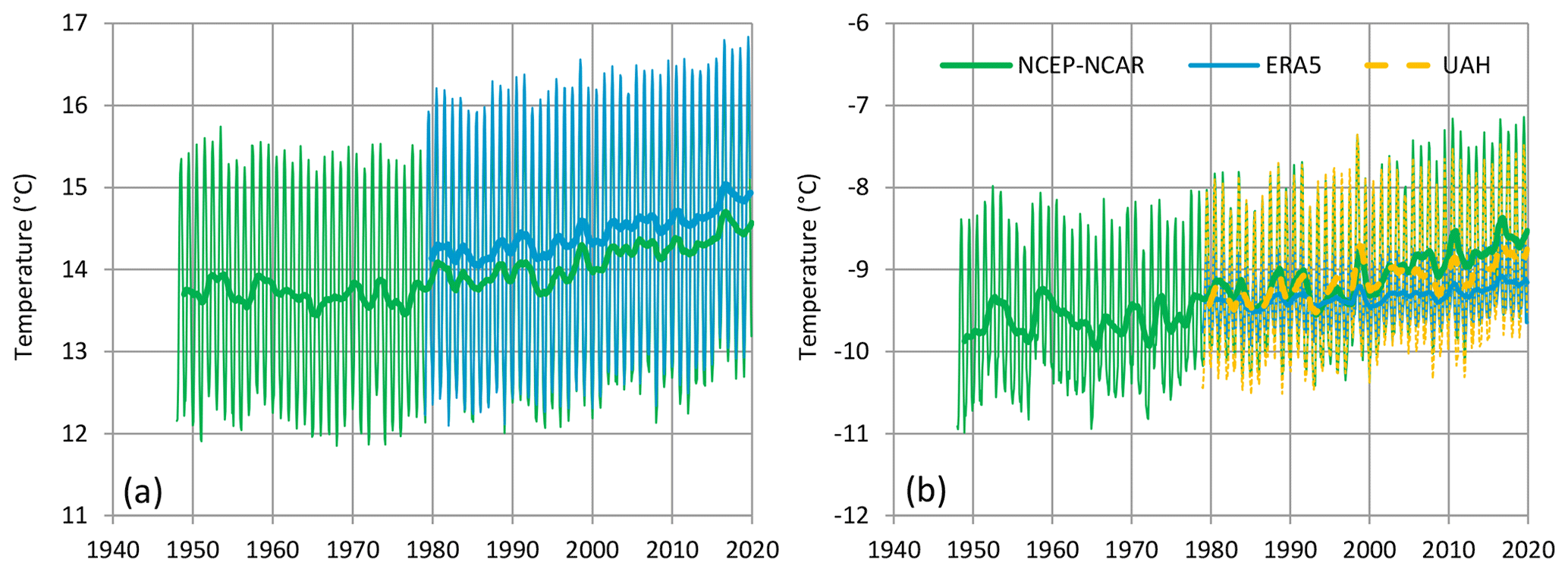
Figure 1Variation of the global average temperature (a) at the level of 2 m above ground and (b) at the lower troposphere. Thin and thick lines of the same colour represent monthly values and running annual averages (right aligned), respectively. Sources of data are indicated in the legend and detailed in Table 1. In panel (b), the reanalyses (NCEP–NCAR and ERA5) time series are weighted averages of those at the levels of 500 and 700 hPa, with weights of 0.62 and 0.38, respectively, which were found for optimal fitting with the satellite (UAH) series.
If we split the common 40-year period into two parts, we may compare the climatic values on a 20-year climatic scale and calculate the temperature increase. This is done in Table 2, where an increase of 0.38 ∘C can be seen for the globally averaged temperature using the ERA5 reanalysis, corresponding to 0.19 ∘C per decade. By reducing the time window of the period defining climate from 20 to 10 years, we can determine the difference of (a 10-year average) climate over 30 years, which is 0.56 ∘C (again 0.19 ∘C per decade). For the UAH satellite data set, which is less affected by urbanization because of the higher elevation, the 30-year difference is lower, namely 0.39 ∘C or 0.13 ∘C per decade.
Table 2Average air temperature (T) and dew point (Td), in ∘C per 20-year and 10-year climatic period, and the resulting differences. Data are from the ERA5 reanalysis, except for lower troposphere, which are from UAH.
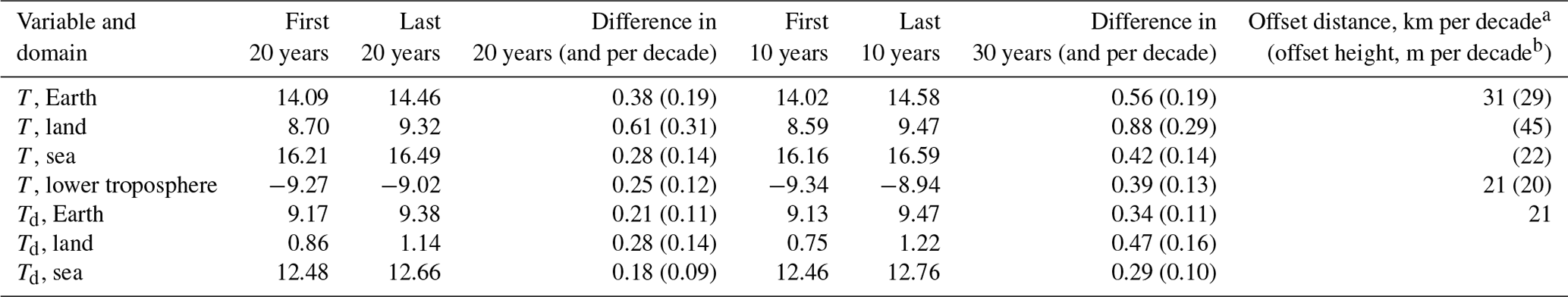
a The distance, which moving poleward in the temperate zone, would
offset, on average, the decadal increase in temperature or dew point.
b The height which, moving up, would
offset the decadal increase in
temperature (assuming a lapse rate of 6.5 ∘C km−1).
In addition, Table 2 provides similar information for the land and sea parts of the Earth, in terms of average temperatures and dew points. The dew point, defined as the temperature at which the air must be cooled to become saturated with water vapour, is a more useful variable than temperature for the study of atmospheric water. The time evolution of both variables on Earth, land and sea, can be seen in Fig. 2. All these are based on ERA5 reanalysis information, as this is the only one readily provided for further processing through the Climexp platform, both for temperature and dew point at the surface level. As a means of verification, the MODIS surface temperature over land is also plotted in Fig. 2, which compares well (albeit with a little bias) with the ERA5 temperature over land. It can be seen in Fig. 2 and Table 2 that the evolution of the dew point is also increasing in the recent period, but the increase is lower than that of temperature.
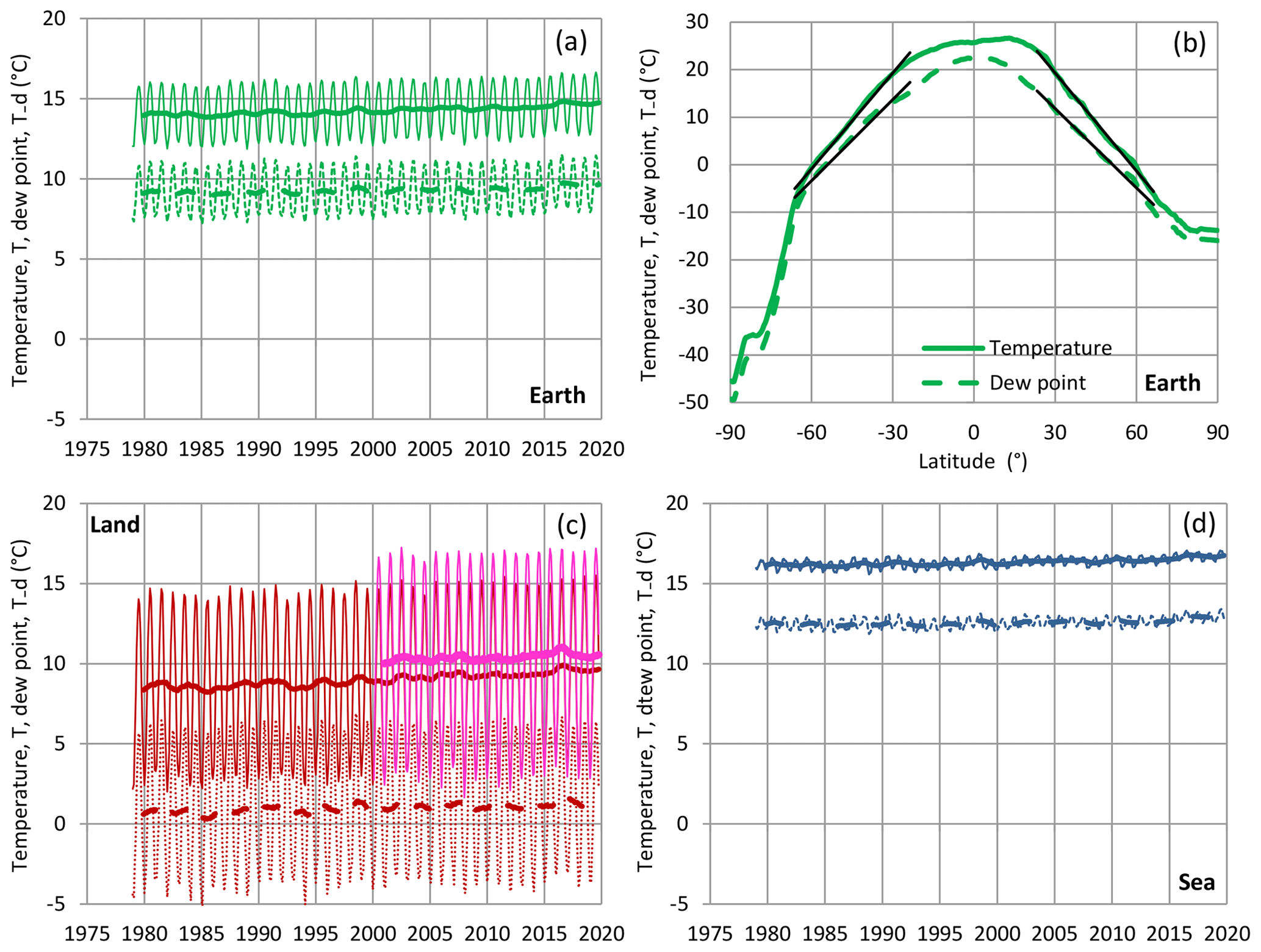
Figure 2(a) Variation of the globally averaged temperature (continuous lines) and dew point (dashed lines) at the level of 2 m above ground. Thin and thick lines of the same colour represent the monthly values and running annual averages (right aligned), respectively. (b) Zonal distribution of Earth temperature and dew point; for the temperate zone (±23.5 to ±66.5∘), the fitted slopes are also plotted (in black), which are ±0.68 ∘C per degree and ±0.56 ∘C per degree, respectively. (c, d) The same as in panel (a) but for the land and sea parts. Source of the data set is the ERA5 reanalysis, as detailed in Table 1; for comparison and validation, in the land graph the MODIS-Terra land surface temperature (averages of daytime and nighttime data sets available since 2000) is also plotted in magenta.
A practical way to express what the increasing rates represent can be obtained by calculating an offset distance on Earth, which, moving poleward in the temperate zone, would offset the average decadal increase in temperature or dew point. This is given in the last column of Table 2 and is 31 km per decade for the surface global temperature and 21 km per decade for the lower troposphere temperature and the surface dew point. This conversion was based on the zonal temperature and dew point profiles shown in Fig. 2b; for the temperate zone (±23.5 to ±66.5∘), the fitted slopes in the profiles are ±0.68 and ±0.56 ∘C per degree, respectively, while one degree of latitude corresponds to 111 km. Another way to express the same is through the height, which, moving up, would offset the decadal increase in temperature, using the lapse rate of the standard atmosphere, namely 6.5 ∘C km−1. As seen in Table 2, to offset the increase in the global Earth temperature, one needs to climb uphill at a rate of 29 m per decade.
It is quite interesting to assess the zonal variation of the increase in temperature and dew point. This information is provided by Fig. 3 where we plot the difference of the Earth temperature and dew point (according to the ERA5 reanalysis) from their averages in the period 1980–1999. A positive difference corresponds to an increase after 1999. It is important to note that the greater increases are located in the northern polar area. In the tropical zone, which is hydrologically most important as the main source of evaporated water, the increase in temperature is half the global average, while there is no increase at all in the dew point. The latter point is of the highest hydrological significance.

Figure 3Zonal distribution of the difference of the Earth temperature and dew point from their averages in the period 1980–1999. Source of the data set is ERA5 reanalysis, as detailed in Table 1. The data for the plot were constructed via Climexp by first computing “anomalies” for the period 1980–1999, then by computing zonal mean and finally by applying the option to “Compute mean, standard deviation, or extremes” and specifying “averaging over 12 months”. Note that the graph represents averages for the entire period of over 40 years, rather than differences between two periods (the latter are about twice the former).
3.2 Humidity
The transition from a temperature-based description of atmospheric processes to a more hydrologically meaningful one is provided by the Clausius–Clapeyron equation, i.e. the law determining the equilibrium of the liquid and gaseous phase of water, which maps temperatures to saturation vapour pressures. Koutsoyiannis (2014b) has highlighted the probabilistic nature of the law by deriving it purely by maximizing probabilistic entropy, i.e. uncertainty. In particular, the law was derived by studying a single molecule and maximizing the combined uncertainty of its state related to the following:
- a.
its phase (whether gaseous, denoted as A, or liquid, denoted as B);
- b.
its position in space; and
- c.
its kinetic state, i.e. its velocity and other coordinates corresponding to its degrees of freedom and making up its thermal energy.
Denoting the saturation vapour pressure as e and using the notion of the so-called natural temperature θ, with units of energy (joules) rather than temperature (kelvins), in accordance with the probabilistic principle that entropy is a dimensionless quantity φ (specifically, with εI denoting thermal energy), the resulting equation is as follows:
where (θ0, e0) are the coordinates of the triple point of water (specifically, θ0=37.714 yJ corresponding to T0=273.16 K, e0=6.11657 hPa), ξ is the phase change energy (the amount of energy needed to break the liquid-phase bonds with other molecules), and βA and βB are the degrees of freedom of a water molecule in gaseous and liquid phase, respectively (specifically βA=6, βB≈18). The same law can be written in more customary notation, in terms of absolute temperature in kelvins and using macroscopic quantities, as follows (Koutsoyiannis, 2012):
where (T0, e0) are again the coordinates of the triple point of water, R is the specific gas constant of water vapour (R=461.5 J kg−1 K−1), , with k as the Boltzmann constant and Na the Avogadro constant, cp is the specific heat at constant pressure of the vapour, and cL is the specific heat of the liquid water. By substituting the various constants, we end up with the following form of the equation (Koutsoyiannis, 2012):
This form is both convenient and accurate (more accurate than other customary forms, theoretical or empirical, as illustrated in Koutsoyiannis, 2012).
A state in which the actual vapour pressure ea is lower than the saturation pressure e(T) is characterized by the relative humidity as follows:
which serves as a formal definition of both the relative humidity U and the dew point Td. Figure 4 depicts the evolution of the saturation water vapour pressures e(T) and e(Td) for the average temperature T and dew point Td, as the latter are shown in Fig. 2, while Table 3 shows their changes per 20-year climatic periods.
Table 3Average vapour pressures, e(T) and e(Td), in hPa per 20-year climatic period, and the resulting differences. Data are from the ERA5 reanalysis.
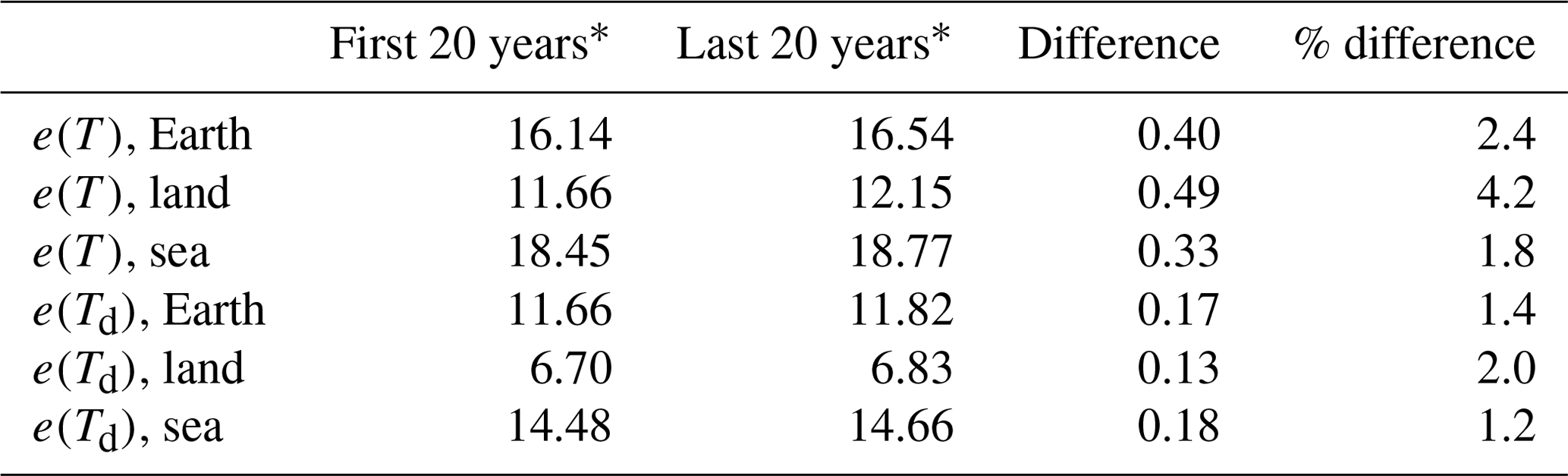
* The values of e(T) and e(Td) were estimated for each time step (month) and then averaged over the indicated period.
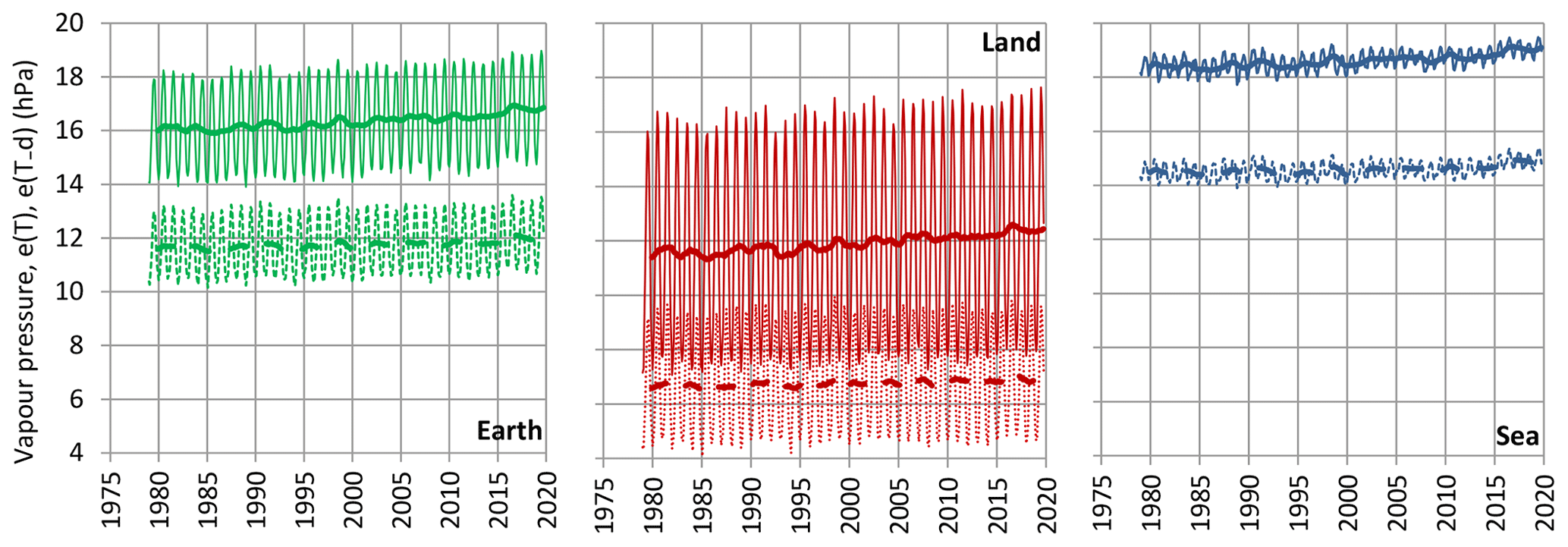
Figure 4Variation of the saturation water vapour pressure e(T) (continuous lines) and e(Td) (dashed lines) for the average temperature T and dew point Td, as shown in Fig. 2. Thin and thick lines of the same colour represent monthly values and running annual averages (right aligned), respectively. Source of the data set is the ERA5 reanalysis, as detailed in Table 1.

Figure 5Variation of specific humidity at the levels of (a, c, e) 850 hPa and (b, d, f) 300 hPa. Thin and thick lines of the same colour represent monthly values and running annual averages (right aligned), respectively. Sources of the data are indicated in the legend and detailed in Table 1.
It is important to note that all the above quantities and derivations do not depend on the presence of other atmospheric gases and, hence, on the air pressure p. To account for the other gases in the air, which constitute the biggest part, known as the dry air, we define the specific humidity as follows:
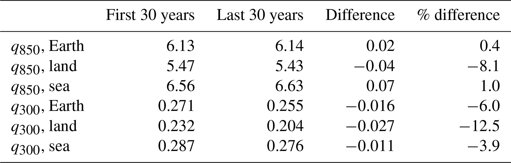
where Mv and Md are the masses of vapour and dry air in a certain volume V, and ρv and ρd are the corresponding densities. The evolution of specific humidity at two atmospheric levels, namely 850 and 300 hPa, according to the NCEP–NCAR and ERA5 reanalyses, is depicted in Fig. 5 for the entire Earth and the land and sea parts. For the 850 hPa level, the two sources of data agree with each other; they indicate fluctuation over time with no monotonic trend. The climatic differences according to the NCEP–NCAR reanalysis are shown in Table 4, where it is remarkable that in the land part at the 850 hPa level the difference is negative. For the 300 hPa level the two sources of data diverge substantially and, most importantly, the NCEP–NCAR suggests a decreasing trend, while ERA5 suggests an increasing trend. We will examine this divergence in Sect. 3.3. Table 4 shows that the change in the NCEP–NCAR data is negative not only on land but also in the sea part and over the entire Earth.
Table 4Specific humidity at 850 hPa (q850) and at 300 hPa (q300) in g kg−1 per 30-year climatic period and the resulting differences. Data are from the NCEP–NCAR reanalysis.
To connect specific humidity to pressures, we use the law of ideal gases, which can again be derived by maximizing probabilistic entropy (Koutsoyiannis, 2014b) and takes the following form:
where p is the pressure and N is the number of molecules. Writing this law separately for water vapour and dry air (eaV=Nwθ, (p–ea) V= (N–Nw) θ, where N is the total number of molecules in volume V of which Nw are water molecules) after algebraic manipulation, we find the following:
where ε is the ratio of the molecular mass of water to that of the mixture of gases in the dry air, i.e. .
It has been a common assumption, based on the Clausius–Clapeyron relationship, that the global atmospheric water vapour should increase by about 6 %–7 % ∘C−1 of warming (e.g. Wuebbles et al., 2017). In turn, this assumption is based on the conjecture that, on the planetary scale, relative humidity will remain roughly constant, and hence, specific humidity is projected to increase in a warming climate (IPCC, 2013, p. 91; see more quotations from the IPCC report in Koutsoyiannis, 2020b). Indeed, combining Eqs. (3), (4) and (7) and considering that e≪ p, we find the following:
It is then easy to verify that for a certain atmospheric level (p= constant) the following relationship holds true:
Under the assumption that U is constant (dU=0), irrespective of the increase in temperature, it is seen that for K, d % dT, while for T=25 ∘C =298.15 K, d % dT, which is in agreement with IPCC.
However, despite the conjecture dU=0 being widely accepted, the real-world data do not confirm it. As we have already seen in Fig. 3, in the tropical area, which is most significant as a source of atmospheric moisture, the dew point (and hence e) remains virtually constant despite the fact that the temperature (and hence e(T)) increases. Clearly, this means that the relative humidity U has decreased with the increase in temperature. This appears to be the case in all of the time series we examined (entries 6 and 7 in Table 1). This result is in agreement with an earlier study by Wang et al. (2008), who concluded that atmospheric temperature and water vapour trends do not follow the conjecture of constant relative humidity over North America.
By combining the time series of relative humidity with those of temperature (entries 3 and 4 in Table 1) and using Eqs. (3) and (4), we constructed in Fig. 6 the vertical profile of the difference of average water vapour pressure e(T) and e(Td)=Ue(T) over land at levels of atmospheric pressure ranging from 1000 to 300 hPa. The focus on the land part of the Earth is justified because most of the hydrological processes are occurring in this part. For the NCEP–NCAR data, the differences plotted in the figure are of 30-year climatic periods, namely 1948–1977 and 1990–2019, and for the ERA5 data of the 20-year climatic periods, namely 1980–1999 and 2000–2019. If the assumption of unchanging relative humidity was valid (dU=0), then the profile of the actual vapour pressure Δe(Td) would be proportional to the saturation water vapour pressure Δe(T), i.e. Δe(Td)=UΔe(T). The resulting curves would then be the dotted lines in Fig. 6 corresponding to the actual Δe(T) of the two periods but with relative humidity, U, estimated from the first climatic period (as it was assumed to be dU=0). However, the real Δe(Td) series depart dramatically from these dotted lines. It is notable that for the NCEP–NCAR data it even becomes negative for a large part of the troposphere (p<700 hPa or elevation >3 km).
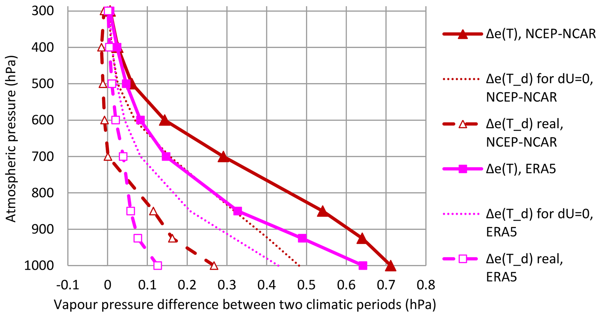
Figure 6Vertical profile of the difference between two climatic periods of average water vapour pressure e(T) and e(Td)=Ue(T) over land at levels of atmospheric pressure ranging from 1000 to 300 hPa. Sources of data: NCEP–NCAR and ERA5 reanalyses as detailed in Table 1 (entries 3–4 and 6–7). For the NCEP–NCAR data, the differences are of the 30-year climatic periods, namely 1948–1977 and 1990–2019, and for the ERA5 data of the 20-year climatic periods, namely 1980–1999 and 2000–2019.
We may try to roughly approximate Eq. (9) by the following:
with a constant parameter, C, which would be 1 if dU=0 held true, but, in fact, it is much lower. Using weighted least squares on the data of Fig. 6, we estimated . This suggests that, contrary to the IPCC (2013) expectation, the global atmospheric water vapour over land is increasing by only about 2 % ∘C−1 of global warming. In this case, we may expect a 4 % increase in atmospheric water in the celebrated (yet contradictory) target of 2 ∘C of global warming. From a hydrological point of view, given the high variability and uncertainty of the processes (see the motto at the beginning of the article), a 4 % change may be deemed negligible. Nonetheless, the analyses that follow indicate that even the reduced rate of 2 % ∘C−1 of global warming may be overestimated, particularly if it is translated into intensification of hydrological cycle.
3.3 Water vapour and cloud water amounts
By integrating the specific humidity over a vertical column of air from a low altitude z0 (typically the surface altitude), corresponding to air pressure p0, to a high altitude z1 (typically the tropopause), corresponding to air pressure p1, we define the (vertically integrated) water vapour amount. Specifically, the water vapour amount is as follows:
where ρw (=1000 kg m−3) is the liquid water density and g (=9.81 m s−1) is the gravity acceleration.
The study of the temporal variation of W is much more informative than q or e because of the vertical integration of information. Both NCEP–NCAR and ERA5 reanalyses provide data for this variable (entries 12 and 13 in Table 1). In addition, we have satellite observations of W (entries 10 and 11 in Table 1), one of which (MODIS) also gives layered information. Figure 7 depicts the evolution of W, according to all sources of information, for the entire Earth and the land and sea parts. The NCEP–NCAR and ERA5 reanalyses agree impressively well with each other; they indicate fluctuation over time with no monotonic trend. The NVAP satellite data also agree on the average, indicating no trend. However, the most recent MODIS satellite data suggest a decreasing trend, just the opposite of the IPCC expectations discussed above. As seen in Fig. 8, which provides layered information for the MODIS data, the decreasing trend is more pronounced in the upper atmospheric levels (440 to 10 hPa). This observation, compared to Fig. 5 and in view of the above discussion (related to Fig. 5 and Table 4) about the divergence of specific humidity trends at 300 hPa between the NCEP–NCAR and ERA5 reanalyses, confirms the former and invalidates the latter. The climatic differences in W according to the NCEP–NCAR reanalysis, which covers a longer (68-year) period, are given in Table 5, where it can be seen that there is a decrease not only in the land part but also on the entire Earth.
Table 5Water vapour amount (W) in mm per 30-year climatic period and the resulting differences. Data are from the NCEP–NCAR reanalysis.


Figure 7Variation of water vapour amount. Thin and thick lines of the same colour represent monthly values and running annual averages (right aligned), respectively. Sources of the data are indicated in the legend and detailed in Table 1. The plotted values for MODIS represent the averages from the Terra and Aqua platforms.
For completeness of the discussion about atmospheric water, Fig. 9 depicts the variation of the cloud water amount in ice and liquid phase according to MODIS satellite data. Again, no monotonic trend is seen. Compared to the water vapour amount (Fig. 8), the cloud water is a very small quantity (2 orders of magnitude smaller).
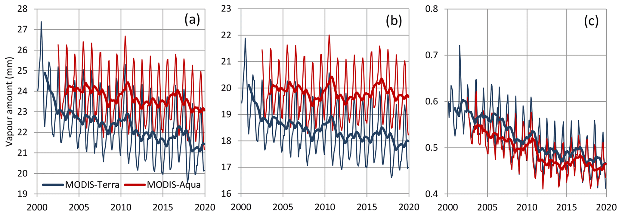
Figure 8Variation of water vapour amount, as in Fig. 7, but only for the MODIS data set and separately for the Terra and Aqua platforms: (a) total of the vertical column, (b) from surface to 680 hPa and (c) from 440 to 10 hPa. Thin and thick lines of the same colour represent monthly values and running annual averages (right aligned), respectively. Sources of the data are indicated in the legend and detailed in Table 1.
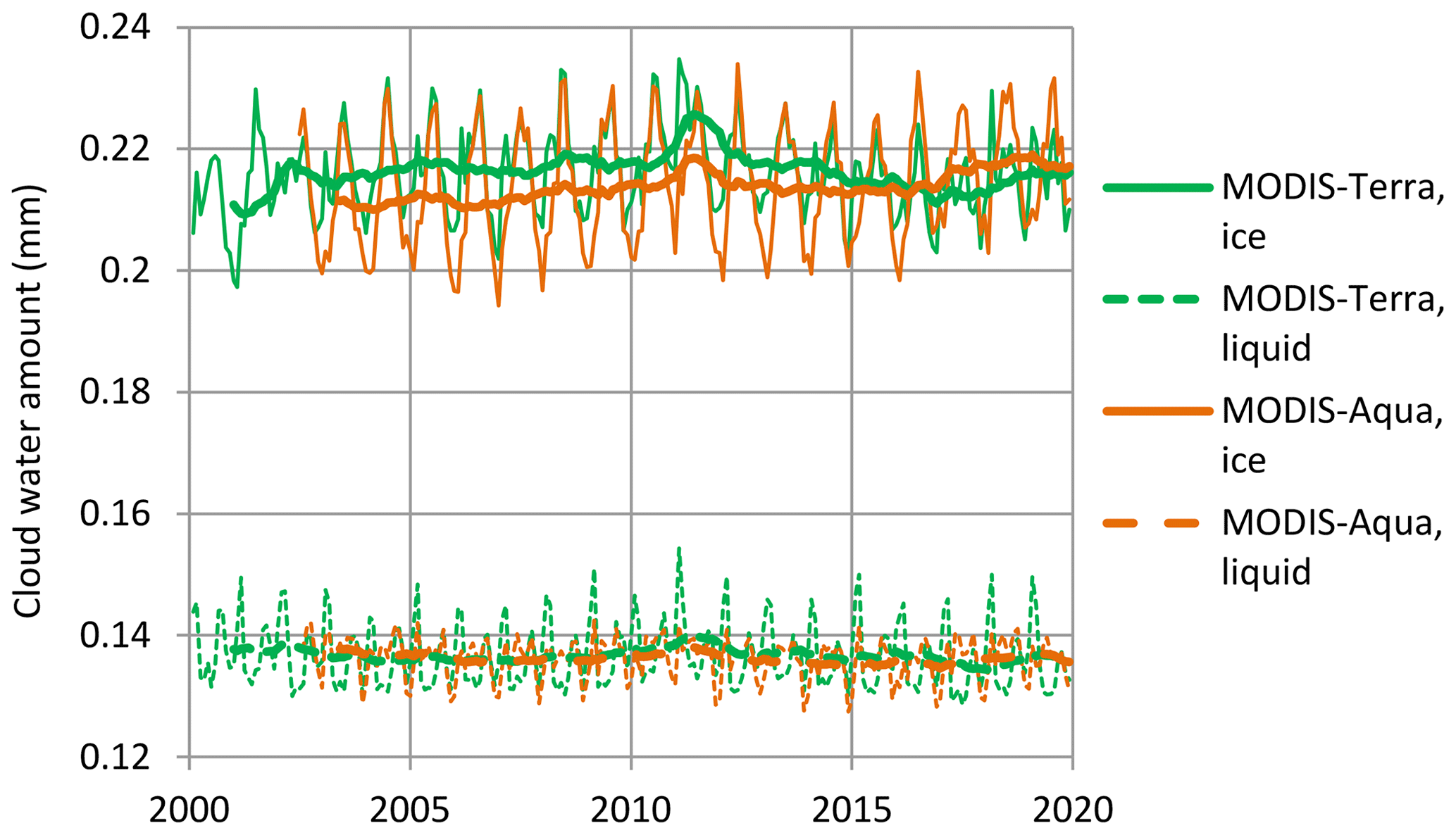
Figure 9Variation of cloud water amount (in ice and the liquid phase). Thin and thick lines of the same colour represent monthly values and running annual averages (right aligned), respectively. Sources of the data are indicated in the legend and detailed in Table 1.
While the analysis of atmospheric water in the previous section signifies potentialities in the hydrological cycle intensity, the analysis of precipitation rate signifies actualities. As already mentioned, the potentiality (the global atmospheric water vapour) was expected by IPCC to increase by about 6 %–7 % ∘C−1 of warming, while the actuality (the precipitation rate) should be lower. Specifically, according to IPCC's latest (Fifth) Assessment Report (IPCC, 2013, p. 91):
It is virtually certain that, in the long term, global precipitation will increase with increased GMST [global mean surface temperature]. Global mean precipitation will increase at a rate per ∘C smaller than that of atmospheric water vapour. It will likely increase by 1 to 3 % ∘C−1 for scenarios other than RCP2.6. For RCP2.6 the range of sensitivities in the CMIP5 models is 0.5 to 4 % ∘C−1 at the end of the 21st century. […] Changes in average precipitation in a warmer world will exhibit substantial spatial variation under RCP8.5.
The rate of increase in precipitation, necessarily accompanied by an equal rate of increase in evaporation, has been known as the sensitivity of the hydrologic cycle (or hydrological sensitivity). The smaller rate, compared to that of atmospheric water, has been estimated based on climate model simulations. Furthermore, Kleidon and Renner (2013; see also Kleidon et al., 2015), based on analytical calculations and thermodynamics, have estimated a hydrological sensitivity of 2.2 % ∘C−1, within the IPCC's “very likely” range. Even when accepting this IPCC assertion, it may be puzzling why hydrologists have given so much energy to studying hydrological impacts that are a priori framed in the range of 1 % to 3 % ∘C−1. For in hydrology such percentages are negligible compared to the natural variability and the uncertainty even in the measurement of precipitation. Moreover, since the potentiality part (the expected increase in atmospheric water) has been already questioned, we may expect that in actuality the changes in precipitation are even less recognizable than those implied by IPCC.
Indeed, Fig. 10, which depicts the evolution of the precipitation rate on Earth and its land and sea parts, based on gauged, satellite and reanalysis information, suggests that precipitation fluctuates through the seasons and also through the years but without a monotonic trend. The marked differences among the various sources of information are also indicative of substantial uncertainty in the estimation of precipitation.
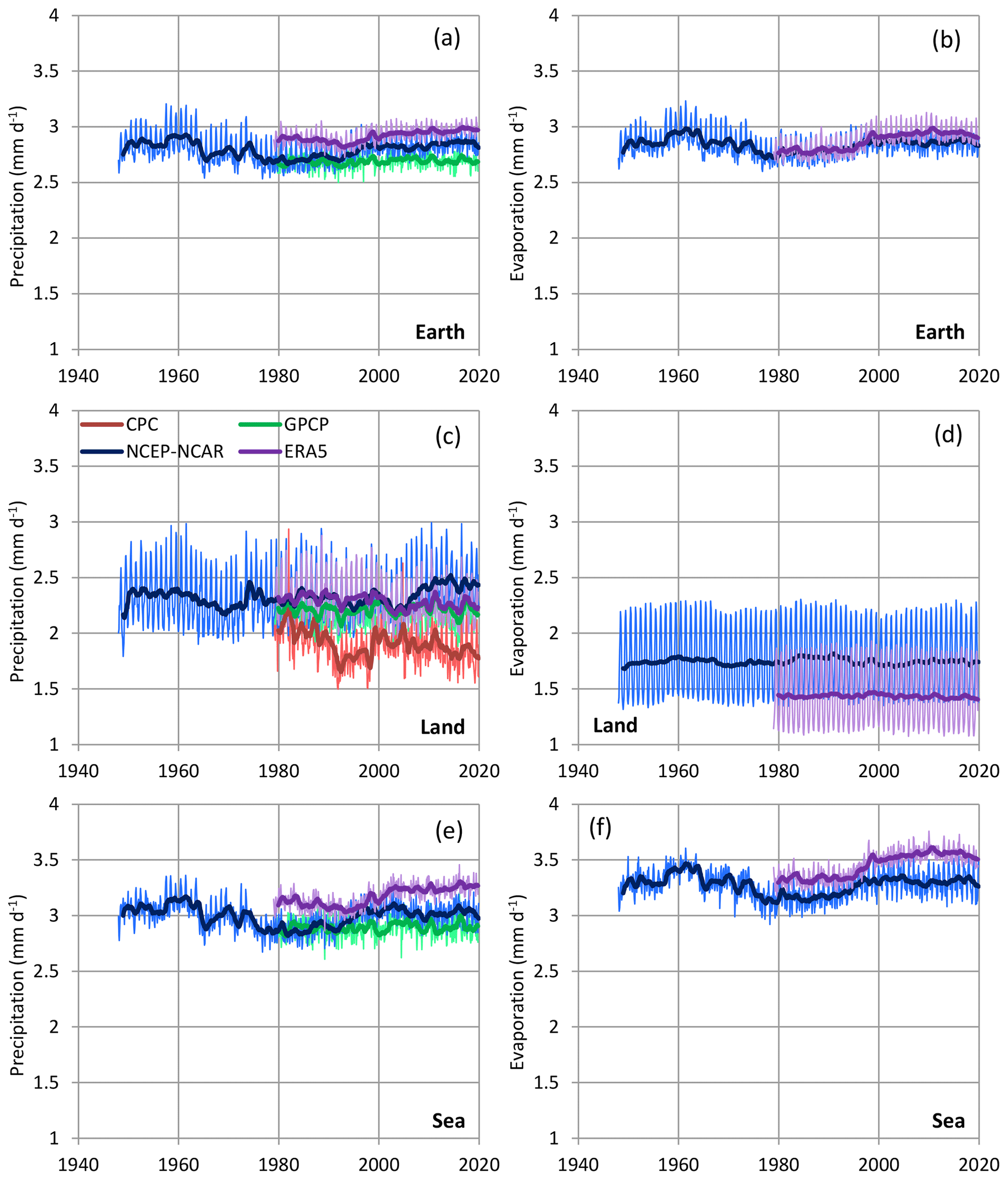
Figure 10Variation of (a, c, e) precipitation and (b, d, f) evaporation. Thin and thick lines of the same colour represent monthly values and running annual averages (right aligned), respectively. Sources of the data are indicated in the legend and detailed in Table 1; GPCP is version V2.3.
The snow part of precipitation is also interesting to examine, as snow is more directly related to temperature. Figure 11 depicts the evolution of the snow cover in the Northern Hemisphere. Despite temperature increases, no noticeable change appears on an annual basis. However, there are perceptible changes in the seasonal variation, namely in the most recent period where the snow cover has decreased during the summer months and increased during the autumn and winter months.
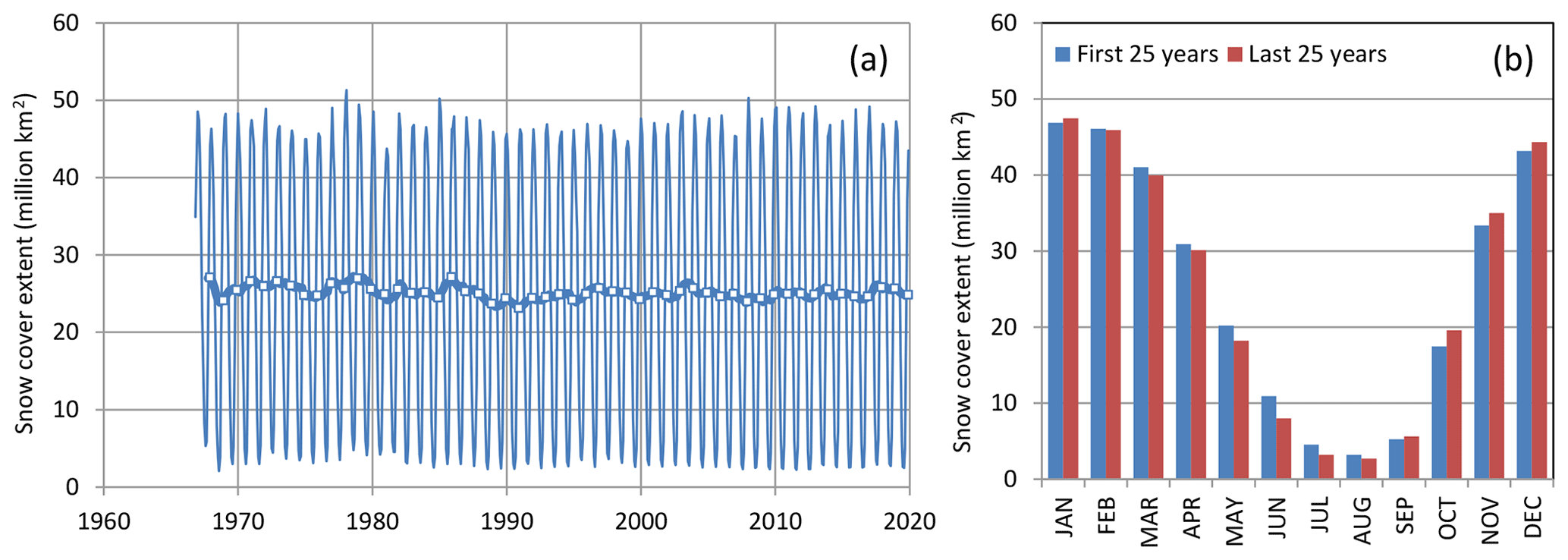
Figure 11(a) Variation of the snow cover extent in the Northern Hemisphere according to GSL; thin and thick lines represent monthly values and running annual averages (right aligned), respectively, and squares are annual averages aligned in December of each year. (b) Seasonal variation of the snow cover, separately, for the first and last 25 years on record.
As already mentioned, the evaporation rate is difficult to estimate and even more difficult to measure. The available gridded data come from reanalyses. Their plots in Fig. 10 again show fluctuations through the seasons and through the years and there are no monotonic trends.
Overall, the preceding data and analyses, particularly those of atmospheric water, can hardly support the intensification of the global hydrological cycle. Certainly, they reveal changes but the changes appear as multi-year fluctuations and not as consistent trends. These fluctuations do not correspond to popular hypotheses attributing changes to global warming. The above results are not exceptionally new. Indeed, Sun et al. (2012) reported a near-zero temporal trend in global mean precipitation for the period 1940–2009. Nonetheless, our results are dissimilar (or opposite) to the vast majority of studies reporting intensification. The reasons for the dissimilarities are explained in Appendix A. Additional analyses, which show the absence of intensification and, more recently, deintensification, in terms of precipitation extremes, are given in Appendix B.
The reasons for the failure of the popular hypothesis of intensification include these two: (a) the unsupported (and eventually falsified) conjecture that the relative humidity should be constant, and (b) the oversimplification of the representation of natural process, which neglects or underrates important mechanisms that affect the atmospheric water more than those related to the greenhouse effect. Among these, mostly unpredictable or unaccounted for, mechanisms are the following: (a) the tropospheric aerosols (Wu et al., 2013) affecting radiation while enabling the condensation of water vapour and formation of cloud droplets; (b) the vapour buoyancy feedback, which stabilizes the tropical climate by increasing the outgoing longwave radiation (Seidel and Yang, 2020)3; (c) the complex role of land use changes in climate (Pielke et al., 2016); and (d) the coupled atmospheric–ocean circulation fluctuations, such as the El Niño–Southern Oscillation (ENSO; e.g. Trenberth et al., 2005, who concluded that the precipitable water variability for 1988–2001 is dominated by the evolution of ENSO and especially the structures that occurred during and following the 1997–1998 El Niño event).
5.1 General framework and assumptions
The analyses of atmospheric water, and those of precipitation and evaporation, reveal the following two important points: (a) all processes fluctuate in time at all timescales, and (b) no monotonic trends that would be attributed to temperature increase appear in any type of data. In some cases (e.g. satellite observations of water vapour amount) there appear to be some trends, which, however, are opposite to established expectations. Here we treat them as irregular fluctuations, which appear as monotonic trends because of the limited time window of the observation. Consequently, in subsequent analyses we make all estimations on the basis of stationarity. It must be stressed that stationarity does not mean the absence of change. It simply means that the change, however large, resists a deterministic description, and hence a stochastic description becomes more appropriate and powerful (Montanari and Koutsoyiannis, 2014; Koutsoyiannis and Montanari, 2015). Additional information on this choice is provided in Sect. 6.2 and 6.3.
A rather impressive result, shown in Fig. 10, is that the precipitation and evaporation over the entire Earth in the NCEP–NCAR reanalysis agree very well with each other, indicating the conservation of mass, a property that is not granted in reanalyses. Indeed, on the annual timescale, the differences between the global precipitation and evaporation are small, ranging between +0.5 % and −4.1 %. This provides a good basis for estimating the water balance in terms of fluxes in the hydrological cycle. The ERA5 reanalysis is not as good, in this respect, as the NCEP–NCAR one. We note, though, that even the small differences on the global scale are amplified when we examine the land and sea separately. This is seen in Fig. 12, which depicts the water balance derived from the difference in precipitation and evaporation at the land and sea. Here the fluxes were converted from mm d−1 used in other analyses to km3 yr−1, considering that the Earth has an area of 510 072 000 km2, of which 28.44 % is land and 71.56 % sea. The amplification of discrepancies (a known effect when taking differences of two processes) is evident in Fig. 12. In particular, the figure shows that the ERA5 reanalysis is, in a systematic manner, far from conserving water mass in the period prior to 2000, but it was much improved in the years 2000–2015 and worsened again in the most recent years. The NCEP–NCAR does not indicate systematic error patterns.
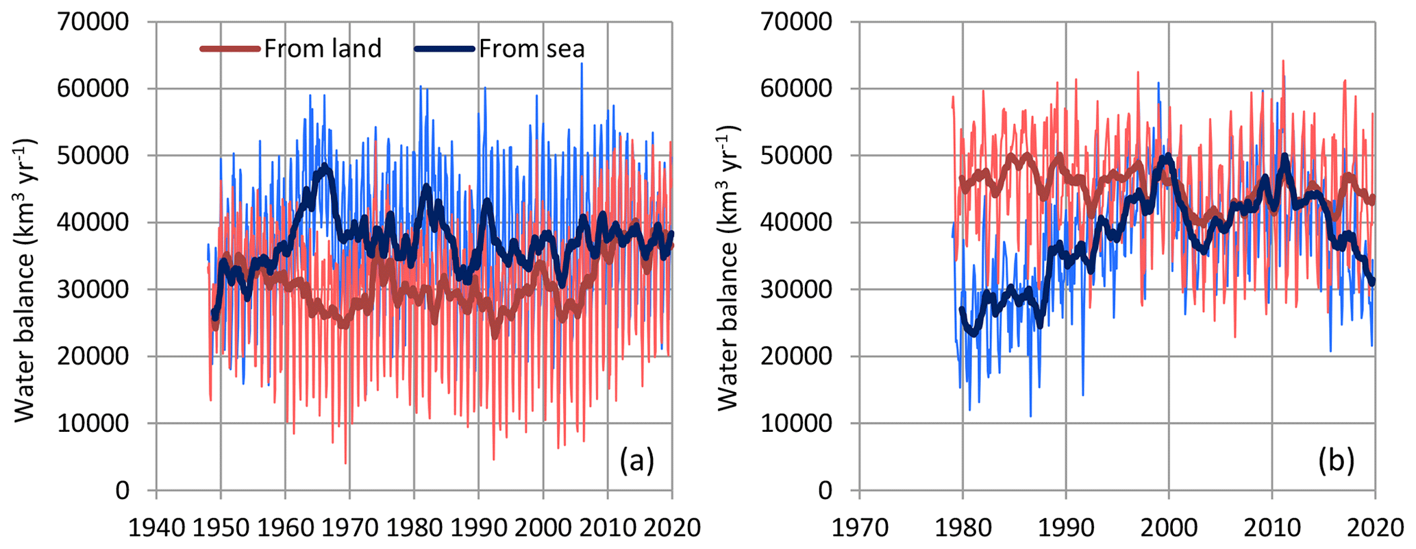
Figure 12Global water balance derived from the difference of precipitation and evaporation at land and sea from (a) the NCEP–NCAR and (b) the ERA5 reanalyses. Thin and thick lines of the same colour represent monthly values and running annual averages (right aligned), respectively.
Before proceeding to water balance estimation, we stress the importance of that balance in quantifying the availability of water resources. Contrary to most other common goods (e.g. fossil fuels and metals) that are subject to depletion, water resources are renewable, not reserves. In this respect, hydrology should fight the common misrepresentation (or even misconception in reports from media and information provided to the wider public and decision makers) implied by the popular use of graphs such as Fig. 13. It is not the purpose of this study to examine or question the correctness of the information in the graph, which shows where on Earth water is stored. However, the graph gives wrong impressions or messages. As an example, it suggests that the vast majority of liquid freshwater on Earth is groundwater, while river water is almost negligible. However, considering the renewable character of water resources, the truth is just the opposite; the vast majority is river water, while groundwater is almost negligible, as will be detailed below. For that reason, a caution stamp is added to Fig. 13.
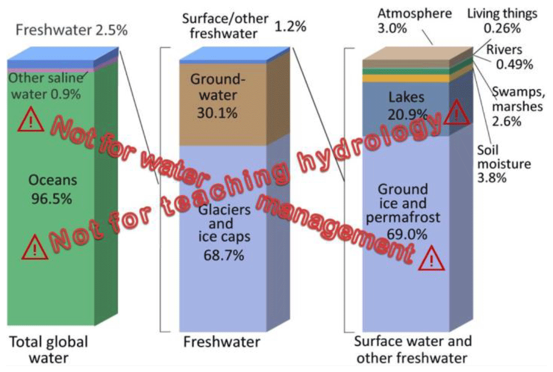
Figure 13Typical depiction of water on Earth (source of the background image without the stamp: USGS; https://www.usgs.gov/special-topic/water-science-school/science/oceans-and-seas-and-water-cycle (last access: July 2020) and Wikipedia: https://en.wikipedia.org/wiki/Water_distribution_on_Earth#/media/File:Earth's_water_distribution.svg, last access: July 2020), with a cautionary stamp added to discourage considering freshwater as non-renewable reserve.
We now proceed to calculations, noting that their precision will be of the order of 100 km3 yr−1; thus, any calculated quantity is rounded off to multiples of this value. The water balance at the land and sea parts of the Earth is written, respectively, as follows:
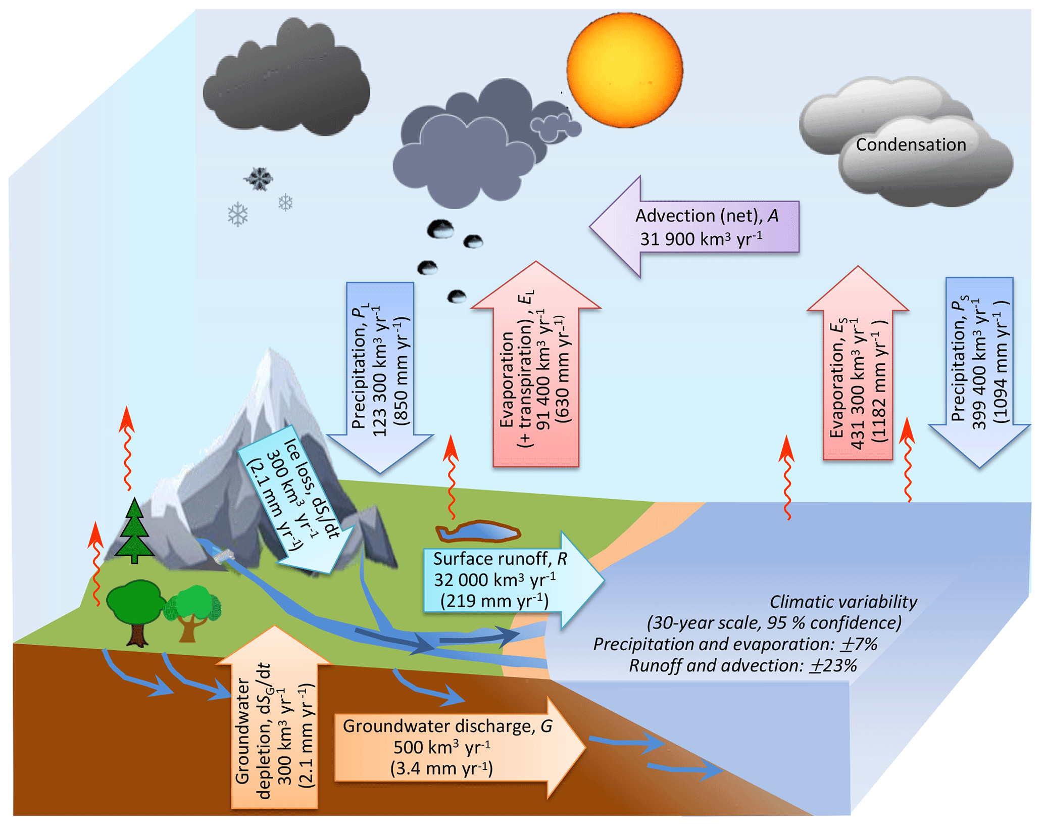
where and are the precipitation flux over the land and sea, respectively; and are the evaporation flux over land and sea, respectively; and are the surface runoff and submarine groundwater discharge to the sea, respectively; and are the storages at land and sea, respectively; and t is time (see Fig. 14). Underlined symbols denote stochastic variables or stochastic processes. Assuming that the water density is 1000 kg m−3 (i.e. neglecting variation due to temperature), the fluxes can be expressed as volumes per time, which in turn are rates multiplied by areas; for example, is the precipitation flux over land [L3 T−1], where is the precipitation rate [L T−1] averaged over land, and AL [L2] is the land area. Assuming zero storage change in the atmosphere (an assumption supported by the analyses of Sect. 3), we can write the following:
Combining Eqs. (12) and (13), we find:
Hence, we can write:
where is the advection, i.e. the flux of water mass from sea to land through atmospheric processes.
5.2 Changes in storage
Changes in land and seawater storage are small but not negligible. With reference to Fig. 13, the land storage can be decomposed into five compartments, namely ice, , snow, , biosphere, , surface water, , and groundwater (including soil water), . Hence, partition the water storage on land as follows:
For the ice loss, Syed et al. (2009), on the basis of the average of two earlier studies, estimated a quantity of km3 yr−1, which refers to Greenland and Antarctica.4 A newer study by Velicogna and Wahr (2013), based on GRACE satellite data, found a change of km3 yr−1 for Greenland and km3 yr−1 (or somewhat larger when using another model) for Antarctica. As noted by Velicogna et al. (2014) the total mass loss is controlled by only a few subregions in Greenland and Antarctica and are mostly due to ice dynamics, where the latter term means the motion within large bodies of ice; this, in turn, is controlled mainly by the temperature and strength of their bases rather than the atmospheric temperature (see also Hanna et al. 2020). However, IMBIE (2020) suggested that in Greenland the shares of losses due to ice dynamics and surface processes are equal (about −75 km3 yr−1 each one; their Table 1 for years 1996–2018). Furthermore, IMBIE (2018; Table 1) estimated for the Antarctic ice sheet a loss of km3 yr−1 for 1992–2017, which becomes km3 yr−1 for 2012–2017 (without specifying the share of ice dynamics). The disagreements among different estimates are highlighted by the results of the study, based on satellite data, by Zwally et al. (2015), who reported that the mass gains of the Antarctic ice sheet exceed losses by 82±25 km3 yr−1 (or somewhat greater, 112±61 km3 yr−1, using a different data set); the study triggered controversy with several comments and replies. Disagreements are also exemplified in Hanna et al. (2020), who, despite the new observational (especially satellite) data and the recent efforts, found that significant discrepancies remain with respect to absolute mass balance values for the East Antarctic ice sheet, while for the Greenland ice sheet absolute values vary by ∼100–300 km3 yr−1 between recent years. In a reconciled estimate for the entire area covered by glaciers, including regions distinct from the Greenland and Antarctic ice sheets, Gardner et al. (2013), using satellite gravimetry and altimetry and local glaciological records, suggested a global budget of km3 yr−1 for 2003–2009. In line with the latter study, here we assume E[ddt] km3 yr−1.
For the snow storage, the snow data analysed in Sect. 4 allow the assumption of a zero mean change at the annual and overyear scales, even though at seasonal scales it is certainly not negligible (see Fig. 11). For the water in the biosphere, there must be a positive change as in the 21st century the Earth has been greening, mostly due to CO2 fertilization effects (Zhu et al., 2016) and human land-use management (Chen et al., 2019). Specifically, the MODIS data show a net increase in leaf area of 2.3 % per decade (Chen et al., 2019), but it is difficult to translate this into a net increase in water stored in the biosphere. Nonetheless, we do not expect this change to be large (in comparison to other changes), and we will neglect it.
Surface water storage has been affected by the substantial depletion of several large natural water bodies in the past, mostly due to overexploitation of their water, while at the same time it was enhanced by the construction of artificial reservoirs. The Caspian Sea changes, often associated with the sea level changes, are large but alternating in sign, i.e. positive or negative (Chen et al., 2017), and thus there is no reason to assume a balance value other than zero. The Aral Sea has dramatically shrunk in volume since 1950 (Gaybullaev et al., 2012; Cretaux et al., 2019) and has thus contributed to a negative water balance in the land (and positive in the sea, corresponding to the rise in sea level), but its stabilization is a likely possibility for the present and future. Reservoir impoundment has also affected the water balance after the construction of reservoirs (Chao et al., 2008). However, given that the number of new reservoirs has diminished after 2000, while a reservoir has zero further effect on the long-term water balance after its first fill, we do not expect further substantial effects.5 For these reasons, we assume a zero (further) change in surface water storage for the contemporary period.
For the groundwater storage change, which we expect to be significant, Wada et al. (2010) have estimated a global depletion rate of 283±40 km3 yr−1 in 2000, which in Wada et al. (2016; their Fig. 1) becomes 292 km3 yr−1 over the period 1900–1999, while Wada (2016; their Fig. 6a) give an estimate of about 200 km3 yr−1 for the year 2000. In their recent review article, Bierkens and Wada (2019) report estimates from several studies, based on global hydrological models and GRACE data, which vary from 90 to 510 km3 yr−1 for the recent years. These justify an average estimate of E[ddt] km3 yr−1 for the contemporary period.
In summary, we have assumed the following:
Accordingly, the water storage in land has a total loss of 600 km3 yr−1, which is a gain for the storage in the sea. This mass gain corresponds to an increase in sea level equal to 1.64 mm yr−1. Half of this (0.82 mm yr−1) corresponds to groundwater depletion (i.e. conversion of groundwater to seawater, as water mass cannot disappear nor can it be stored in the atmosphere, where it initially moves by evaporation in irrigated areas). This is clearly an anthropogenic effect in its entirety and is likely to remain, if not increase, in the foreseeable future. It is also a clear mark of unsustainable water management. An equal portion of the rise in sea level (0.82 mm yr−1, according to this study) is due to ice loss from land, but, as already mentioned, most of it is not attributed to anthropogenic causes. The latter value is consistent with the estimates by Marzeion et al. (2015), which range between 0.70 and 0.96 mm yr−1 for the period 2003–2009. For comparison, an almost equal amount, 0.77 mm yr−1 according to Llovel et al. (2014), or higher, 1.31–1.32 mm yr−1 according to WCRP (2018), is due to thermal expansion. One may hastily tend to attribute this latter amount to anthropogenic global warming, neglecting natural variability (including the succession of El Niño/La Niña events). Such negligence may be problematic; for, undoubtedly, neither the 125 to 140 m rise in sea level in the last 20 000 years (Fleming et al., 1998) nor the sea level change from a range of up to 600 m in the last 500 million years (Hallam, 1984; van der Meer et al., 2017) are anthropogenic.
5.3 Submarine groundwater discharge
The submarine groundwater discharge (or groundwater outflow to the sea) is the most difficult to estimate. A most recent estimation has been conducted by Zhou et al. (2019) using a water budget approach at high resolution. They examined the near-global coastal recharge areas (60∘ N to 60∘ S) and provided spatially distributed high-resolution estimates using average infiltrating runoff from three land surface models (MOSAIC, NOAH and VIC) obtained from NASA's GLDAS. They concluded with a near-global estimate of submarine groundwater discharge at 489±337 km3 yr−1, noting that 56 % is the export in tropical coasts, while mid-latitude arid regions export only 10 %. In line with this recent estimate, here we assume the following:
This choice needs some further explanation, as it is substantially (by 4–5 times) lower than the commonly adopted earlier estimates, such as those by Shiklomanov and Sokolov (1985) and Zekster and Loaiciga (1993; citing Zektser and Dzhamalov, 1981), which are 2200 and 2400 km3 yr−1 in the two studies, respectively, or about 5 %–6 % of total runoff; the latter quantity had been estimated to 46 800 and 38 000 km3 yr−1 in the two studies, respectively.
An even earlier, yet frequently cited, estimate by Lvovitch (1970), is somewhat lower, namely 1600 km3 yr−1. Lvovitch did not obtain this estimate himself but cites Nace (1964), who suggested it, also noting that he finds it reasonable. Surprisingly, however, in another article, Nace (1967) clearly states that this value is arbitrary. Specifically, his footnote to “ground-water outflow to oceans” in his Table 1 (which, notably, mixes water stocks and fluxes) is, verbatim, “Arbitrarily set equal to about 5 percent of surface runoff”. In addition, it seems that Nace has made a numerical error as the value he gives for surface runoff is 38 000 km3 yr−1; hence, 5 % thereof is 1900 km3 yr−1 rather than 1600 km3 yr−1.
These old guesses, rather than estimates, have been adopted (by citing the above studies) in most papers and textbooks until now, either in its percentage version (e.g. 5 % in Dai and Trenberth, 2002, who cite Lvovitch, 1970) or in absolute values, mostly adopting Shiklomanov and Sokolov's (1985) values of 2200 and 46 800 km3 yr−1 for the groundwater and total runoff, respectively (Dingman, 1994; Khedun and Singh, 2017).
Values even higher than those have also been published; for example, in a celebrated paper, Oki and Kanae (2006) assert the following:
some part of the water, approximately 10 % of total river discharge (Church, 1996), infiltrates to deep underground and will never appear as surface water but discharge into the ocean directly from groundwater.
And, indeed, Church (1996) contains this 10 % estimate, but also refers to a wide range, between 1 % and 10 %, without performing his own analyses. He further implies that the 10 % estimate was proposed by Zektzer et al. (1973). However, this value in Zektzer et al. refers to the groundwater discharge to the Lake Ladoga and, coincidentally, to some results for the United States by Nace (1969). In general, the review and methodological paper by Zektzer et al. (1973) does not contain any information on the global scale.
The only case of a low estimate, of the order of that used here, is in Nace's (1970) paper, which appears to be the first quantitative analysis in history of the groundwater discharge to the sea. Surprisingly, only 3 years after his 5 % arbitrary set guess, Nace (1970) came up with the quantitative estimate of 7000 m3 s−1, or about 220 km3 yr−1, that is 7–9 times smaller (depending on the correction or not of his aforementioned error) than his own initial guess. Subsequently he remarks:
The average total runout [i.e. submarine groundwater discharge] then would be about 7000 m3 s−1. This is less than 1 percent of estimated surface runoff. While the calculation is wholly hypothetical, it is based on liberal assumptions. In order to be significantly large the value would have to be greater by a factor of 5. Evidently, runout is negligible in relation to the world water balance, though it is significant within some regions.
It is thus likely that behind the initial 5 % guess, and its eager adoption by later researchers, was a desire for the value “to be significantly large”. However, one may think that such an overestimation of the groundwater flux, in addition to overemphasizing the groundwater stock (which appears very large in Fig. 13), may have offered bad service both to science and water management, as it may have encouraged the overexploitation (far beyond the natural recharge rate) of groundwater, with consequences such as the subsalinization of coastal aquifers, the subsidence of land areas and the rise in sea level. The quotation and the whole story may also be didactic as they illustrate the adverse consequences of convictions about what the values would have to be, otherwise known as confirmation biases.
The fact is that the estimate of 220 km3 yr−1 has remained unnoticed in the literature. The general preference has been to quote, misquote or confirm the 5 % guess, as indicated in the above references. To complete this timeline of consistent distortion, the following excerpt from Zhou et al. (2019) is quite indicative:
Integrated over the near-global coastline, the total annual volume of fresh SGD [submarine groundwater discharge] is 489 km3/year ± 337 km3/year, or 1.3 % of river discharge (Dai & Trenberth, 2002), in line with previous estimates (Church, 1996; Zekster [and] Loaiciga, 1993).
While, as already stated, here we fully adopt the estimate of Zhou et al., which is closer to Nace's (1970) estimate than to any other, the authors' assertion that their value of 1.3 % is in line with those they cite (which as explained above is 5 % to 10 %, or 4 to 8 times larger, even though Church mentions the 1 % case) is surprising. Perhaps a statement such as the above, which hides big disagreements among estimates, hinders the discussion of an important issue. Without an extensive discussion the issue remains open; hopefully the analysis here has shed some light, but it is not the scope of this article to resolve this open problem.
5.4 Final quantification of water balance
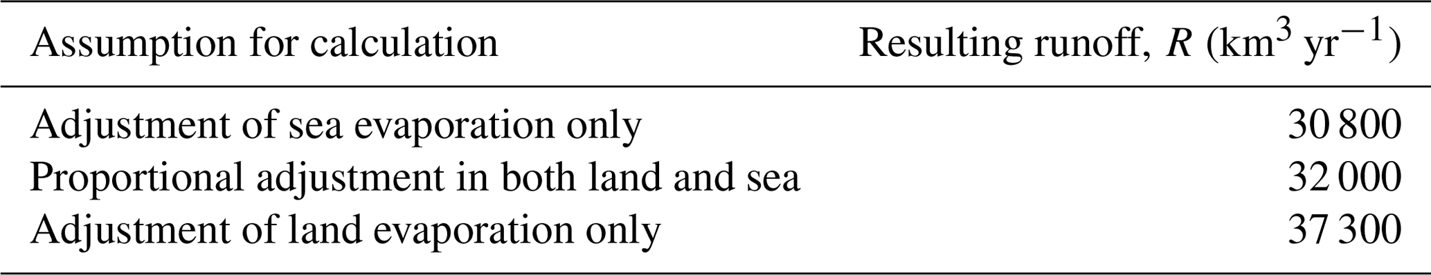
The above detailed review and discussion was about small quantities in water balance. Fortunately, the big quantities, namely precipitation and evaporation over the land and sea, are estimated more accurately (on a percentage basis), and the NCEP–NCAR reanalysis provides a good basis for estimation. As already stated, the error in satisfying Eq. (14) is +0.5 % and −4.1 % on the annual scale. Given the above assumptions, the unknown quantities are the runoff R and the advection A. Their expectations will be as follows:
while, with the numerical values assigned to the last three terms in the former equation, we will have km3 yr−1.
To proceed, we assume that the precipitation values are more reliable, as they are cross-checked with satellite data, and we adjust the evaporation data so as to precisely satisfy Eq. (14). A sensitivity analysis of the effect of allocating the error in the resulting water balance is shown in Table 6. If we allocate the entire error to sea evaporation, the resulting mean runoff is 30 800 km3 yr−1, while if we allocate it to land evaporation it increases to 37 300 km3 yr−1. However, a proportional adjustment to both land and sea seems more reasonable. In this case, the resulting average runoff is 32 000 km3 yr−1 and the advection 31 900 km3 yr−1. All these quantities are graphically illustrated in Fig. 14. The figure also includes information on the climatic variability on a 30-year climatic scale of the averages given; explanations about the values noted will be given in Sect. 6.3. We stress that variability does not coincide with uncertainty. The former corresponds to the fact that climate is varying. While climatic variability translates to uncertainty when future predictions are cast, there are additional sources of uncertainty, such as errors in the data and assumptions.
If we apply Eq. (19) and drop the expectations, i.e. use the time-varying values, what we will get is not the actual runoff and advection because some storage changes not included in the equation, such as in snow, soil water and atmospheric water, are not identically zero; rather, their mean is zero. On the annual basis it may be expected that the error is negligible, but on the monthly scale it will be present. Nonetheless, such an exercise is useful to conduct to see the temporal variability. This is depicted in Fig. 15, where, for rigour in terminology, we have replaced the terms “runoff” and “advection” with “water balance from land” and “water balance from sea”, respectively. Figure 15b depicts the mean monthly averages, which differ remarkably. The differences are related to the within-year storages not included in the equation and look quite reasonable. As the Northern Hemisphere dominates in land processes, it is reasonable to expect that in the period December–May the storage is increasing, while during July–October it is decreasing.
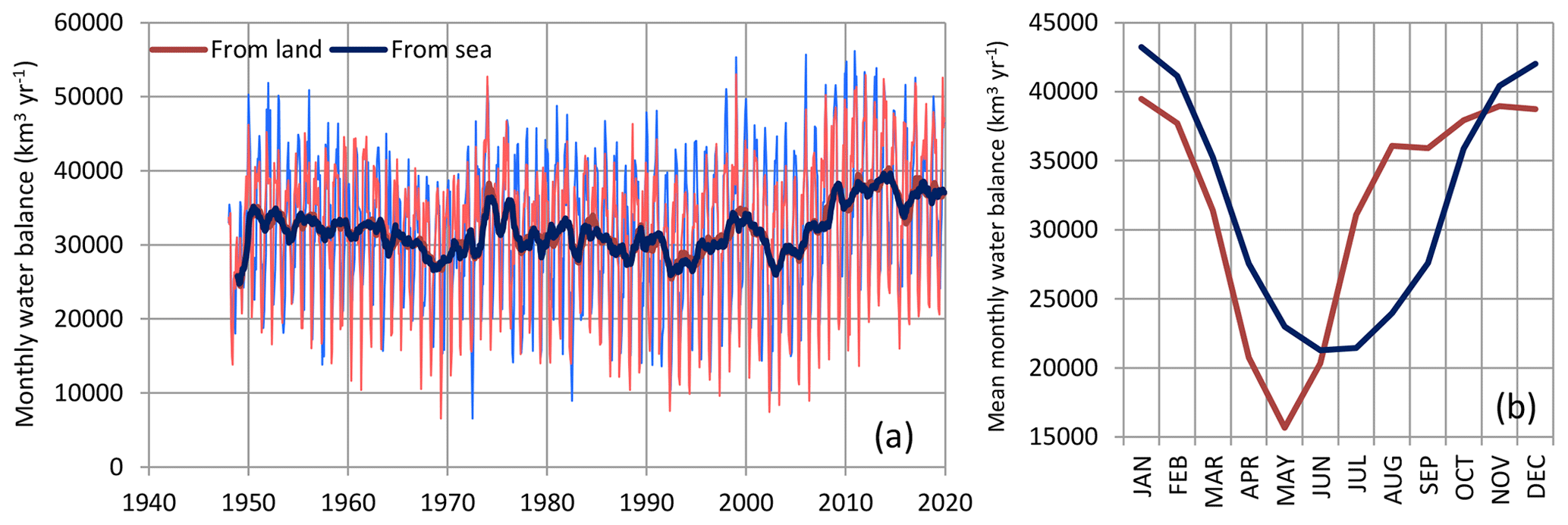
Figure 15(a) Final global water balance on land and sea from the NCEP–NCAR reanalysis. Thin and thick lines of the same colour represent monthly values (but with rates expressed in km3 yr−1) and running annual averages (right aligned), respectively. (b) Average seasonal variation of the water balance.
Compared to the popular estimates by Shiklomanov and Sokolov (1985) and Zektser and Dzhamalov (1981), which, as already noted, are 46 800 and 38 000 km3 yr−1, respectively, our estimate of mean total (surface and groundwater) runoff of 32 500 km3 yr−1 is markedly lower. However, it is (almost precisely) equal to the estimate by Syed et al. (2009; their Table 6), which is based on observed terrestrial water storage changes from GRACE and reanalysis data. The latter study (Syed et al., 2009; their Table 5) also quotes older estimates, from 1975 onwards, which range from 22 000 to 40 000 km3 yr−1. A newer monography by Dai (2016) provides an estimate at about 36 500 km3 yr−1, which is very close to the estimate by Zektser and Dzhamalov (1981) and to the value 38 450 km3 yr−1 estimated by Ghiggi et al. (2019), based on GRUN for the period 1902–2014; the latter authors also report results from earlier studies ranging from 30 000 to 66 000 km3 yr−1. On the other hand, the recent study by Schellekens et al. (2017) suggests a value of about 46 300 km3 yr−1, which is very close to that of Shiklomanov and Sokolov (1985). According to Schellekens et al. (2017), the terrestrial precipitation is 119 700 km3 yr−1 (compared to 123 300 in the present study) and the evaporation 74 500 (compared to 91 400 in the present study); thus, it is the difference in evaporation that makes the latter study inconsistent with the present one.
Figure 16 provides a comparison of runoff time series (or balances in the land and sea) from the present study with earlier studies. The differences in estimates are apparent and translate to a huge uncertainty about the true value of runoff. What is also apparent is a satisfactory agreement between the present study and that of Syed et al. (2009). Some of the studies provide ensemble values, but in Fig. 16 only the ensemble means are plotted (the upper limits of the ensembles would exceed the plotting area). In view of the high uncertainty, it seems not meaningful to search for trends in runoff. We may notice, though, that in the time series of the present study, there appear higher values in recent years. These values correspond to increased rainfall in NCEP–NCAR reanalysis over land. This, however, is not confirmed by the gauge and satellite observations (Fig. 10), which, as already discussed, indicate falling trends. Therefore, the changes will be interpreted as irregular fluctuations within a frame of very high uncertainty rather than monotonic trends which clearly are not.
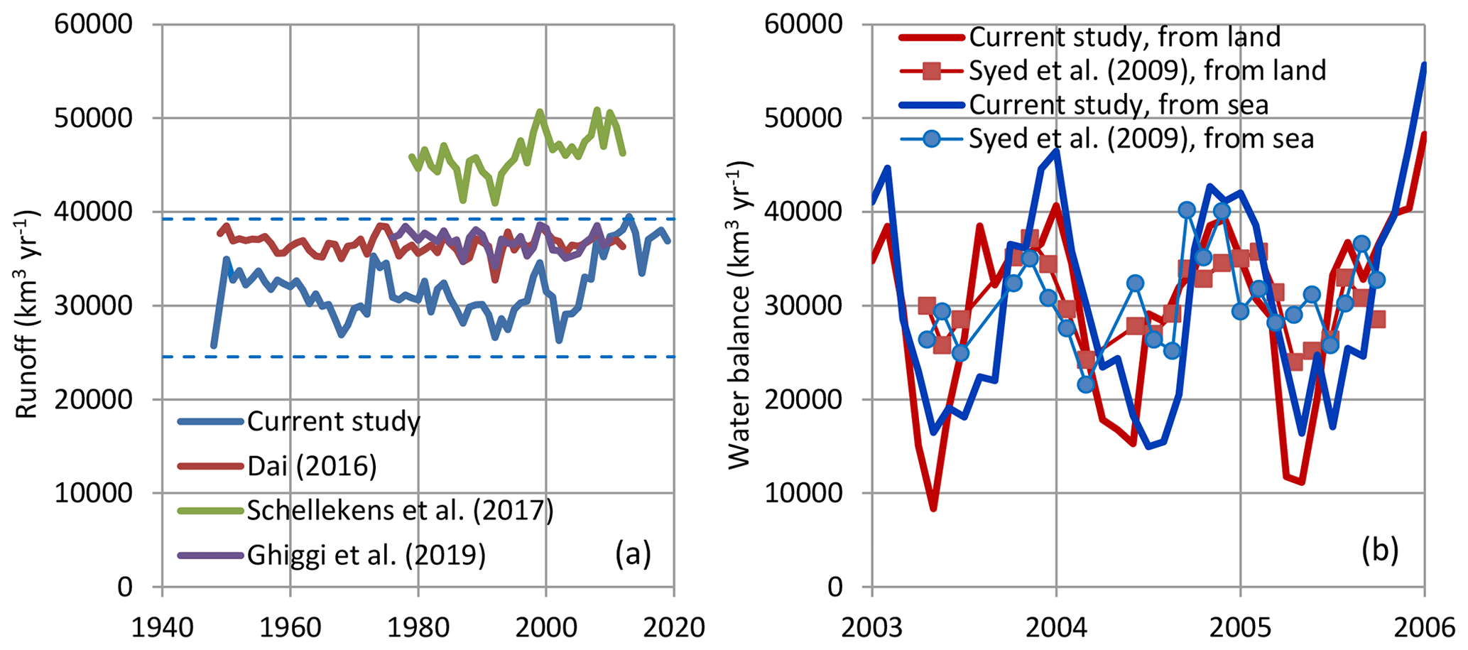
Figure 16Comparison of the results of the current study for surface runoff with those of (a) Dai (2016; Fig. 2.8; digitized), Schellekens et al. (2017; Fig. 7; digitized; ensemble mean), Ghiggi et al. (2019; Fig. 8a; digitized; ensemble mean) at the annual scale and (b) Syed et al. (2009; Fig. 7; digitized) at the monthly scale (but with rates expressed in km3 yr−1). Dashed lines in (a) are the 95 % confidence limits of the 30-year climatic average of the current study.
The latter interpretation is consistent with the results of a large-scale study of trends in the flow of 916 of the world's largest rivers by Su et al. (2018). The results, and specifically those in their Table 1 that take into account the long-term persistence, show some trends that are either positive (3.7 % of the rivers) or negative (8.2 % of the rivers). While negative trends are more frequent than positive, they have slightly lower slopes, so that, overall, the positive slopes slightly surpass the negative ones in magnitude (9.1 vs. −7.2 hm3 yr−1).
5.5 Energy involved in the hydrological cycle
According to Fig. 14, the total evaporation on Earth (precisely equal to the total precipitation according to Eq. 14) is 522 700 km3 yr−1 and corresponds to 5.227×10¹⁷ kg yr−1 of water flux. For the average temperature of Earth equal to 14.46 ∘C (Table 2), the latent heat of evaporation (calculated from Koutsoyiannis, 2012; Eq. 40) is 2.467×10⁶ J kg−1. Thus, the total energy involved in the hydrological cycle is 1.290×1024 J yr−1 or 1290 ZJ yr−1. This corresponds to 4.086×10¹⁶ W, which, if reduced to the Earth's area (5.101×10¹⁴ m2), results in an energy flux density of 80 W m−2 that is precisely equal to the value given by Trenberth et al. (2009). This is about half the global solar energy absorbed by the Earth (161 W m−2, according to Trenberth et al., 2009).
Compared to the human energy production, which in the past decade was about 170 000 TWh yr−1 or 0.612 ZJ yr−1 (corresponding to the year 2014; Mamassis et al., 2020), the total energy involved in the water cycle is 2100 times higher. Put differently, the total human energy production in 1 year equals the energy consumed (or released) by the hydrological cycle in about 4 h.
6.1 Deterministic approaches: climate model predictions vs. data
While most climate impact studies have been based on the assumption that climate models provide plausible predictions (usually termed “projections”) of future hydroclimate, there are a number of studies that claimed that this cannot be true as, when compared with real data of the recent past (after the predictions were cast) or even earlier data (already known at the time of casting the prediction), they prove to be irrelevant with reality (Koutsoyiannis et al., 2008, 2011; Anagnostopoulos et al., 2010). This becomes even worse if we focus on extremes (Tsaknias et al., 2016). Tyralis and Koutsoyiannis (2017) developed a theoretically consistent (Bayesian) methodology to incorporate climate model information within a stochastic framework to improve predictions. However, because of the bad performance of the climate models, application of this methodology leads to increased uncertainty or, in the best case, to results that are indifferent with respect to the case where the climate model information is not used at all. In summary, as implied by Kundzewicz and Stakhiv (2010), climate models may be less “ready for prime time” and more ready for “further research”.
To test if this is also the case on a global setting, here we use climate model outputs for monthly precipitation simulations for scenario runs for the period 1860–2100, from the Coupled Model Intercomparison Project (CMIP5), a standard experimental protocol for studying the output of coupled atmosphere–ocean general circulation models (AOGCMs). CMIP5 includes the models for the IPCC Fifth Assessment Report (https://esgf-node.llnl.gov/projects/cmip5/, last access: February 2020). The scenario used is the already mentioned “RCP8.5” (frequently referred to as “business as usual”, even though there is a lot of controversy about this, e.g. Burgess et al., 2020). The model outputs have again been accessed through the Climexp platform (option Monthly CMIP5 scenario runs).
A comparison of model outputs with reality, as the latter is quantified by the satellite (GPCP) observations, is provided in Fig. 17. As expected by the assumptions and speculations mentioned in Sect. 3, climate models predict an increase in precipitation after 1990–2000. This hypothetical increase is visible in Fig. 17. However, real-world data do not confirm the increase. What is also noticeable is the large departure from reality of model outputs in terms of the average global precipitation. All these observations support the claim that climate models dissent from the hydrological reality and they further illustrate the fact that the real-world precipitation has not been intensified according to the IPCC expectations.
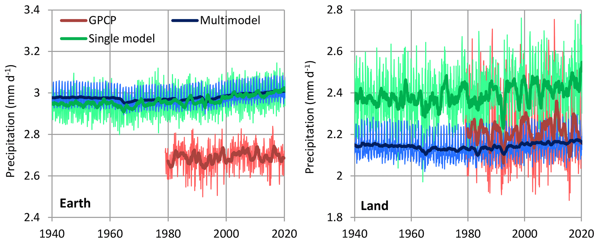
Figure 17Comparison of climate model outputs (for the specification of which, see the text) with reality, as quantified by GPCP satellite observations. “Multimodel” refers to CMIP5 scenario runs and entries, namely CMIP5 mean – RCP8.5. “Single model” refers to the ensemble member 0 of the Community Climate System Model version 4 (CCSM4) – RCP8.5 released by NCAR. Thin and thick lines of the same colour represent monthly values and running annual averages (right aligned), respectively.
6.2 Statistical approaches: trends
The statistical counterpart of the endeavour to predict the future, namely the fitting of trends everywhere, based on real data, and projecting them to the future, has been quite popular among hydrologists in the 21st century, as seen in a surge of related articles. Specifically, this has been quantified by a bibliometric investigation by Iliopoulou and Koutsoyiannis (2020), who show that in the last decade almost 90 % of the scientific articles related to precipitation, hydrology and extremes contain the word “trends”.
The comprehensive study by Iliopoulou and Koutsoyiannis (2020) assessed the “trends everywhere” approach using long precipitation series (>150 years). The study compared four cases of projection to the future, namely (a) the mean estimated from the entire record, (b) a local time average estimated from the recent past, (c) a linear trend fitted to the entire record, and (d) a local linear trend estimated from the recent past. The mean of the process is a neutral predictor of the future (zero efficiency), but it turns out to be better than predictions based on trends. In other words, the predictive skill of the trend model is poor, worse than using the mean, reflecting a poor representation of a complex reality. The model based on the local time average (case b) of previous years proves to be the best of the four. The reason is that in real-world processes there is temporal dependence or persistence (see below). Hence, a local temporal average (of values of the recent past) can be a better predictor than the global (or the true) mean.
6.3 Stochastic approaches: Hurst–Kolmogorov dynamics
The failure of climate models and trends to describe reality does not imply that in reality there is no change. On the contrary, all data sets examined suggest change, but the simplistic assumption that there is virtually a single cause (i.e. CO2 concentration increase) that produces change does not work. Also, the other simplistic assumption that a trend seen in the past will continue in the future cannot work either, as it manifests misrepresentation of stochastic patterns as deterministic trends, while the stochastic patterns should formally be described in terms of time dependence. More generally, history shows that attempts to foretell the unknown future within a deterministic paradigm results in spectacular failures. Therefore, in the real-world hydrological practice there has been a legacy of using stochastics, which reflects a different paradigm in both understanding and modelling natural processes (Koutsoyiannis et al., 2009; O'Connell et al., 2016).
Assuming that a real-world process xτ is modelled as a stochastic process , where τ denotes discrete time, we can monitor the changes at multiple timescales κ through the following time-averaged process:
For small κ (e.g. daily scale), we usually call “weather” and for large κ (e.g. corresponding to 10, 30 or more years) we call it “climate”. We may notice that there is no qualitative difference between weather and climate. Both are varying in time, and the variation is quantified by the variance γ(κ) as a function of timescale κ, which is a function termed the “climacogram” (Koutsoyiannis, 2010). For sufficiently large κ (theoretically as κ→∞), we may approximate the climacogram as follows:
where H is termed the Hurst parameter. The theoretical validity of such (power type) behaviour of a process was implied by Kolmogorov (1940). The quantity 2H−2 is visualized as the slope of the double logarithmic plot of the climacogram for large timescales. In a random process, , while in most natural processes , as first observed by Hurst (1951). This natural behaviour is known as (long-term) persistence or Hurst–Kolmogorov (HK) dynamics. A high value of H (approaching 1) indicates enhanced presence of patterns, enhanced change and enhanced uncertainty (e.g. in future predictions). Additional information on the relationship of Hurst–Kolmogorov dynamics with change can be found in Koutsoyiannis (2013), while the applicability of the law (21) to timescales as long as several million years can be seen in Markonis and Koutsoyiannis (2013).
Now, Fig. 18 shows the climacograms of the different types of processes examined in this study and the different sources of information. It is evident that all processes are consistent with the HK dynamics. Seasonality also has a significant effect in some (but not all) of the processes. In most of the processes H is very high, namely 0.9 or even higher. A notable exception is GPCP precipitation time series with H=0.64. However, the NCEP–NCAR precipitation suggests much higher variability at all timescales and H close to 0.90.
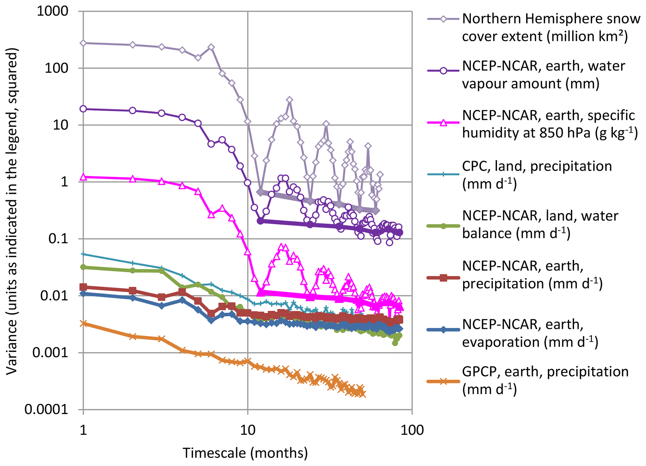
Figure 18Climacograms of the indicated processes calculated from the monthly time series; for some series with prominent seasonality the climacograms from the annual time series are also plotted with thicker lines of the same colour. For timescales greater than the annual, all slopes in the double logarithmic plots are close to −0.2, suggesting a Hurst parameter of 0.90 (or larger, if bias is taken into account). Exceptions are the NH snow cover extent with a slope of −0.47, suggesting a Hurst parameter of 0.76, and the GPCP precipitation series with a slope of −0.72, suggesting a Hurst parameter of 0.64.
High H values imply high climatic variability; assuming that the discrete timescale κ represents years and that the law (21) is a good approximation for the annual and multi-year scales (an assumption verified in Fig. 18), we can conclude that the climatic variability at scale κ, expressed through the coefficient of variation, is as follows:
For κ=30 and H=0.9, this implies a 30-year climatic variation equal to 71 % of the annual variation, while this would be 18 % if the process were random (if H were 0.5). Additional information on the consequences of the HK behaviour in changing our perception and modelling of climate can be found in Koutsoyiannis and Montanari (2007) and Koutsoyiannis (2011).
Arguably, climate has been changing for the entire 4.5-billion-year history of the Earth; this has already been confirmed and roughly quantified for the last 0.5–0.75 billion years in aforementioned studies (Markonis and Koutsoyiannis, 2013; van der Meer et al., 2017). A changing climate can hardly be described by a mean value; variability also needs to be specified. For this specification we certainly need a measure of variation, which could be one of the standard measures (variance, standard deviation or coefficient of variation). But we also need to define how this variability decreases as the timescale increases. A parsimonious way of doing the latter task is through the Hurst parameter, which, based on the data sets used, turns out to be very high, implying that the difference between weather and climate is not as dramatic as the common perception. In this respect, even if the established climatic hypotheses of an intensifying hydrological cycle, with rates of the order of 1 %, were validated, hydroclimatic concerns would not be justified. In older times such rates of change would not be discussed at all, as the logical framework about precision was already formed in ancient times (see the motto in the beginning of the article).
In fact, the established climatic hypotheses on the hydrological cycle are not validated by the data analysed. Relative humidity is decreasing in the entire atmosphere instead of being constant. Specific humidity is increasing at a rate of about one-third of that implied by established hypotheses, which results from comparing two recent periods of the climatic timescale. When integrated over the entire troposphere and viewed in continuous time, the water vapour amount is fluctuating without a monotonic trend, while there are differences even in the sign of local trends for different data sets. Precipitation and evaporation again fluctuate. The precipitation extremes and their frequencies also fluctuate (Appendix B). Fluctuations are successions of intensification and deintensification, with deintensification prevailing in the 21st century.
The water balance on the land and sea appears to be lower than the standard figures of literature. The total evaporation on Earth, precisely equal to the total precipitation, is estimated at 522 700 km3 yr−1 and corresponds to a total energy flux of 1290 ZJ yr−1 or 80 W m−2. The surface runoff is estimated to be 32 000 km3 yr−1, while the submarine groundwater discharge appears to be only 1.5 % of runoff or 500 km3 yr−1. The variability in climatic timescales of all water balance components is very large, in accordance with Hurst–Kolmogorov stochastic dynamics. The uncertainty in figuring out the global water balance is still high, despite the recent big data amounts. The sources of uncertainty are many and, as analysed in the study, need substantial additional efforts to quantify. The most obvious anthropogenic signal in the hydrological cycle is the overexploitation of groundwater, which has a visible effect on the rise in sea level. Melting of glaciers has an equal effect, but in this case it is not known which part is anthropogenic as studies of polar regions attribute mass loss mostly to ice dynamics.
The above observations strengthen an earlier (Koutsoyiannis et al., 2009) envisagement of the hydrological community's role. Instead of a passive role in assessing hypothetical hydrological impacts based on doubtful climate model outputs, an active role consistent with its history is possible. Indeed, hydrology has much more to offer to societies than prophesies of future catastrophes (cf. Koutsoyiannis, 2020a). During the 20th century, and particularly after the Second World War, hydrology, by supporting hydrotechnology, water management and risk assessment and reduction, within a strong international collaboration and a strong economy, has substantially contributed to human life as a value and to the quality and length of human life (Appendix B; Fig. B5).
We clarify that here, to detect possible intensification in the hydrological cycle, we use past information on the global scale. This is similar to the common practice of detecting global warming, where the temporal evolution of an observed, globally averaged, temperature is typically used. While the globally averaged temperature is a statistical quantity with doubtful physical meaning, the globally (or regionally) averaged precipitation and evaporation are physically meaningful as they represent fluxes of water mass or volume. Therefore, it may be puzzling as to why the same method used in temperature has not been applied to precipitation, yet intensification claims have been the norm. This methodology of testing the alleged intensification of the hydrological cycle distinguishes this study from the plethora of other studies claiming intensification. More specifically, the differences in the current study with other studies include the following points.
- 1.
We do not refer to model projections for the future which predict intensification (like e.g. Ziegler et al., 2003; Madakumbura et al., 2019). And, indeed, as evident in Fig. 17, if we used the climate model simulations and not the actual data, we would “detect” intensification even for the past years, let alone the future in which the model-projected increase in rainfall is higher. There are plenty of reasons why one should avoid that, with these reasons referring both to the past and the future. In general epistemological terms, according to Bridgman (1966), when a statement purports to be about the future, it is a pseudo-statement. In more technical terms, it has been shown that the skill of climate models for representing hydrological processes (in particular, precipitation), measured by studying the past performance, is practically zero (Koutsoyiannis, 2008, 2011; Anagnostopoulos et al., 2010; Tsaknias et al., 2016). This situation is epitomized in the title of the article by Stephens et al. (2010), as being a “dreary state of precipitation in global models”.
- 2.
We investigate the entire period that each data set allows in order to see the patterns of changes, i.e. whether there are monotonic trends or fluctuations. If one focuses on a short period (like in the study of Wild et al., 2008, which is for 15 years), it is likely that one would obtain a monotonic trend (even though in Fig. 1 of Wild et al., 2008, consistent increasing appears for 8 years, and not for the entire 15-year period they examine).
- 3.
We do not refer to specific regions like Canada (Déry et al., 2009; Creed et al., 2015), the Amazon (Gloor et al., 2013), etc. Certainly, there are regions where precipitation is currently intensifying, while in earlier periods in those regions, or in other regions at the same period, are deintensifying. Even the cited studies speak about trend reversals in time or give alternating trend signs in different locations. Such temporal and spatial fluctuations, rather than monotonic trends, are normal behaviour in natural processes (see Sect. 6.3). Furthermore, we do not focus on specific seasons of the year. There is no doubt that in certain areas and in specific seasons one would find intensification or deintensification. However, as the spatial scale and observation period increase, the risk of a false claim of intensification decreases. For example, in their recent study based on 1427 stations across China over the last 60 years, Wang and Sun (2020) concluded that there is no significant difference in the annual precipitation between the past 20 years (1999–2018) and the past 60 years (1959–2018) and suggest utilizing the historical data of annual precipitation as the basis for water-resources application.
- 4.
We use a simple and easily reproducible methodology and provide all the information for the reproducibility of the results. The quantities we use are observable or estimated quantities, as given in the original data sets, without making any post-processing or transformation (e.g. probability-based indices based on fitted distributions or regression on “signals”, like in Paik et al., 2020), which could involve subjective choices.
- 5.
We follow Aristotle's advice (to “look for precision in each class of things just so far as the nature of the subject admits”; see the motto at the beginning). For example, an alleged 2 % total increase in the precipitation over land during the entire 20th century (Huntington, 2006, and references therein) is far beyond the precision of estimating precipitation over land.
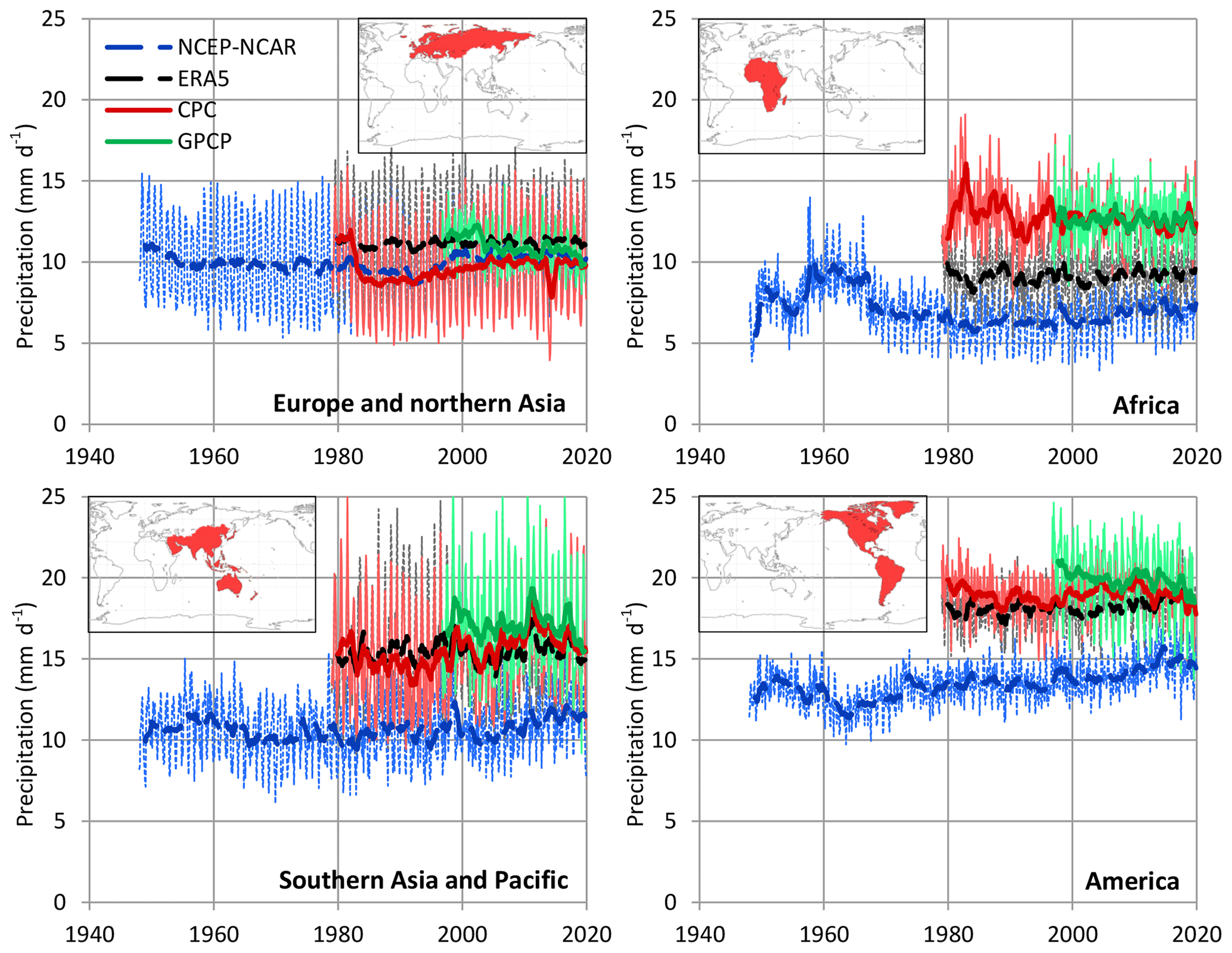
Figure B1Variation of the monthly maximum daily precipitation areally averaged over the continents. Thin and thick lines of the same colour represent monthly values and running annual averages (right aligned), respectively. Dashed lines are for reanalyses and continuous lines for observations. Sources of the data are indicated in the legend and detailed in Table 1.
While, as articulated in Sect. 4, intensification of the global hydrological cycle can hardly be supported on the basis of global precipitation and evaporation fluxes, a large body of literature attempts to re-establish intensification on the basis of extremes. There is no shortage of studies that diagnose such intensification. To refer to just one example, the results of Donat et al. (2016), and specifically those in their Fig. 1 referring to the annual maximum daily precipitation, show some increase in the recent decades, which perhaps inspired their article title, namely “More extreme precipitation in the world's dry and wet regions.” However, when examining their graphs, it is seen that the climatic value of annual maximum daily rainfall of the 30-year period of 1980–2010, compared to that of 1960–1980, is greater by 5 % for dry areas and by 2 % for wet areas. These percentages may perhaps not be meaningful to a hydrologist who deals with real-world planning and design. Also, specifying particular areas such as dry and wet (which are subjectively defined and in the above study represent a small portion of the globe) and neglecting others, may distort the entire global picture.
Extremes are connected to disasters. A shortage of disasters has never been the case, but our perception of them is driven less by disasters per se and more by the communication thereof. In this respect, one may notice increasing trends, both in reporting disasters to the general public and in the production of research articles on disasters. Such articles typically focus on particular areas recently hit by disasters. California is a popular example but not the only one. Evidently, if we choose at random, say, 12 000 sites on Earth, then every month we will have, on the average, one catastrophic event of a 1000-year return period in one of the sites. The roots of the intensification of disaster reporting belong to the domains of psychology (cf. the notion of “availability bias”) and sociology rather than of hydrology. Thus, Blöschl and Montanari (2010) note:
There may also be a sociological element to the interpretation of flood trends which we term as the hydrologist's paradox: A recent large flood in a catchment will often lead to funding a study on the flood history of that catchment which will find there was a large flood at the end of the record. Simultaneously analysing many catchments in a large region will help reduce the chances of these self-fulfilling prophesies.
This social behaviour of targeting research to deal with recent disasters, which however lose societal focus after some time, has been also known as the “hydro-illogical cycle”, a term attributed to Vit Klemes (Kundzewicz et al., 1993) but perhaps used earlier by others (Anderson et al., 1977).
As a result of the intensification of disaster reporting, people think that rainfall events have become more intense or frequent recently. However, based on a list of world record point precipitation measurements compiled by Koutsoyiannis and Papalexiou (2017) for various timescales ranging from 1 min to 2 years, the fact is that the highest frequency of record rainfall events occurred in the period 1960–1980; later the frequency was decreased remarkably.
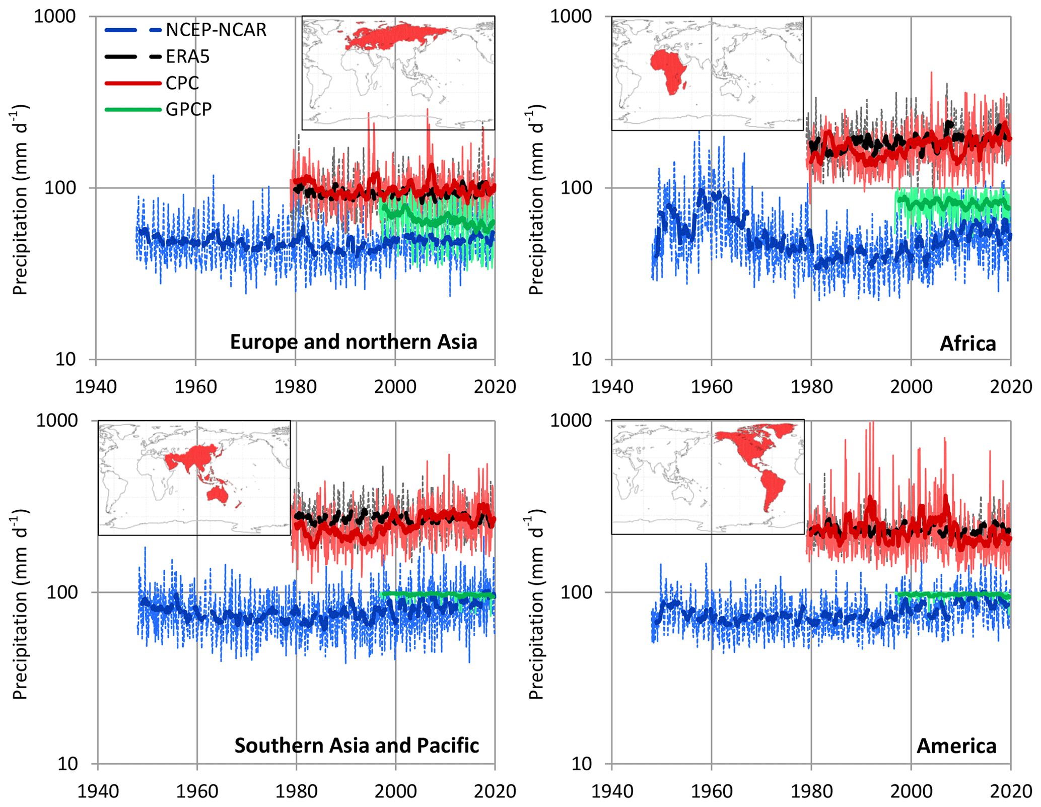
Figure B2Variation of the areal maximum, over each continent, monthly maximum daily precipitation. Thin and thick lines of the same colour represent monthly values and running annual averages (right aligned), respectively. Dashed lines are for reanalyses and continuous lines for observations. Sources of the data are indicated in the legend and detailed in Table 1. Notice that the satellite (GPCP) data do not seem to capture precipitation rates higher than 100 mm d−1.
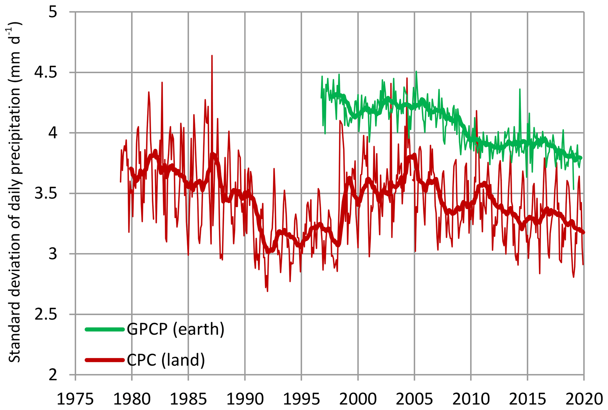
Figure B3Variation of the standard deviation of daily precipitation in each month, areally averaged. Thin and thick lines of the same colour represent monthly values and running annual averages (right aligned), respectively. Sources of the data are indicated in the legend and detailed in Table 1.
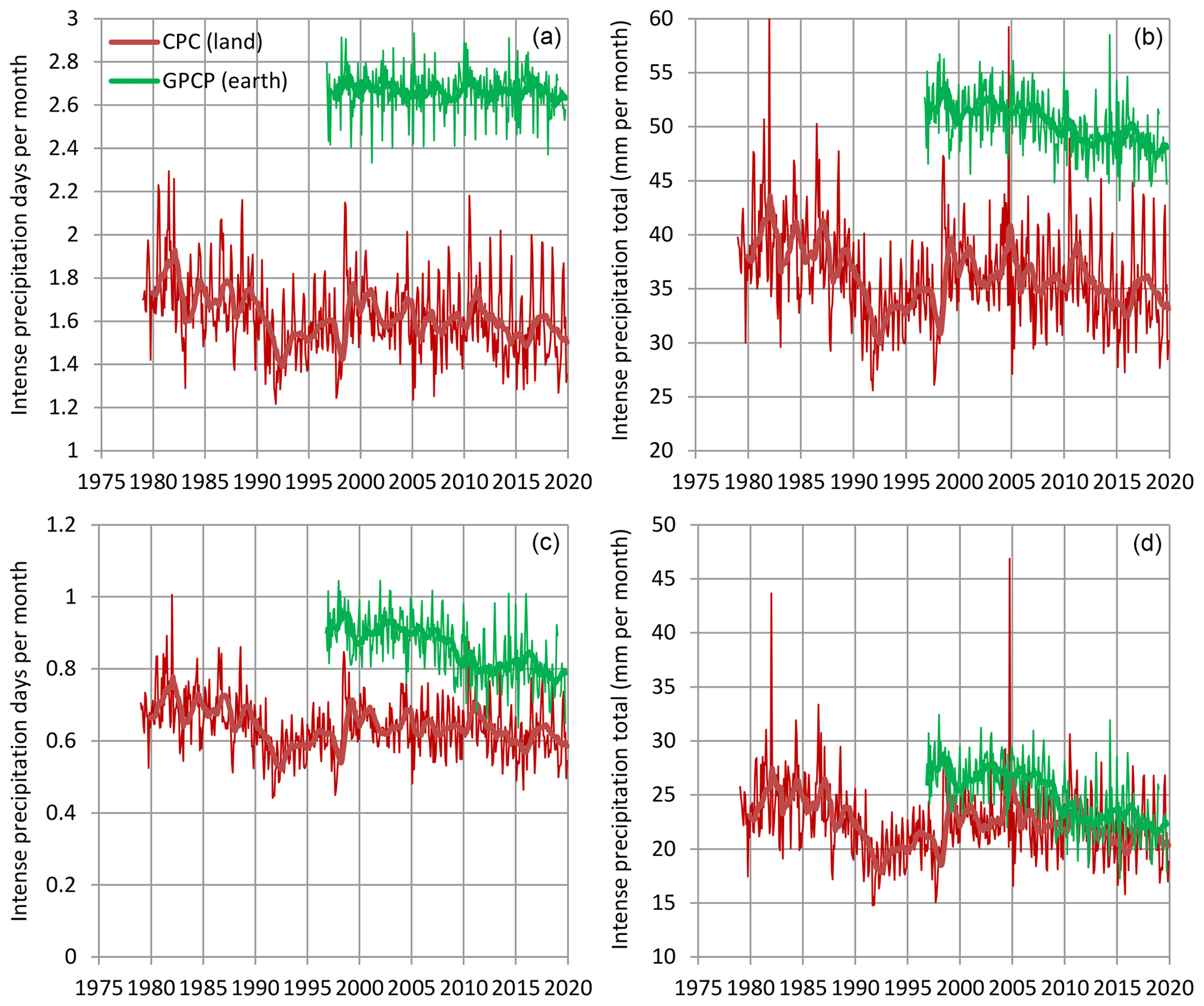
Figure B4(a, c) Average days per month with precipitation exceeding a threshold value, which is 10 mm d−1 for the upper row and 20 mm d−1 for the lower row; (b, d) monthly total of daily precipitation exceeding the threshold value. Thin and thick lines of the same colour represent monthly values and running annual averages (right aligned), respectively. Sources of the data are indicated in the legend and detailed in Table 1.

Figure B5Evolution of the frequency of deaths from floods and droughts per decade in the 20th and 21st century. For comparison, deaths from other categories of natural catastrophes are also plotted: “extreme weather” includes storms, extreme temperatures (cold- or heatwave, severe winter conditions) and fog; “earthquake” also includes tsunamis; “other” comprises landslides (wet or dry), rockfalls, volcanic activity (ash fall, lahar, pyroclastic flow and lava flow) and wildfires. For the sources of the data, see entry 23 in Table 1.
A more detailed analysis can be based on the four sources of daily rainfall information analysed here. This analysis has been performed separately for each continent, and its results are presented graphically. Figure B1 shows the temporal evolution of the monthly maximum daily precipitation areally averaged over the continents. Figure B2 shows similar information but for the areal maximum, over each continent, monthly maximum daily precipitation. None of the figures in none of the continents and none of the sources of data provides support on the intensification allegation. In particular, the observational data (CPC and GPCP) could support the opposite hypothesis, namely that of extreme rainfall deintensification. This becomes even more evident if we examine the temporal evolution of the standard deviation of daily precipitation in each month averaged over the land. In this respect, Fig. B3 shows that deintensification, expressed as decreasing standard deviation, is evident in the 21st century both from CPC and GPCP observational data. This confirms an earlier result by Sun et al. (2012) who, using global, land-based () observations in seven monthly databases, “Unexpectedly […] found a reduction in global land [precipitation] variance” and concluded that “on average, the dry became wetter while wet became drier”. A similar result is shown in a different manner in Fig. B4 in terms of the precipitation rate exceeding a threshold. Clearly, neither the frequency of high precipitation nor the sum of high-intensity precipitation is intensifying. Rather, in most of the cases, there has been deintensification in the 21st century. Again, however, it will be more prudent to speak about fluctuations rather than deintensification. This confirms that stationary models (but with appropriate dependence structure; see Sect. 6.3) should also be used for extremes, as also pointed out by De Luca et al. (2020).
Even if, on a climatic basis, there was intensification at percentages like 1 % or 5 % mentioned above, casting catastrophic prophesies about the future, would be a misleading approach. The real data on the impacts of disasters of climatic type suggest a spectacular drop in the severest of them since the beginning of the 20th century. Figure B5 summarizes relevant information for victims of natural disasters. The sources of the data are seen in Table 1 (entries 22 and 23). The climate-related victims (particularly those from floods and droughts) have diminished, while other types of disasters, such as earthquakes, still have large numbers of victims. Obviously, the reason behind such diminishing is not that floods and droughts have become less severe or less frequent. Rather it is the fact that in the 20th century, instead of casting pessimistic prophesies about the future, societies improved hydrotechnology, water management and risk assessment and reduction, while strengthening international collaborations and the economy, so that the advances could be actually implemented.
All data used in the study are freely available as described in the article and in particular in Table 1, which provides all the required links.
The author declares that there is no conflict of interest.
I am grateful to the colleagues who have put their huge data sets online, as well as the data processing systems they developed. This has been the most important development in hydrology and geophysics since the time I entered academia several decades ago, to which I too have consistently tried to contribute in my country, with only partial success. I have started this research on the occasion of four invited lectures and seminars during 2017–2019 in Lunz, Palermo, Moscow and Bologna (eventually cancelled). I thank the colleagues who invited me or were involved in any respect with the organization of the talks: Dario Braga, Alexander Gelfan, Tatiana Fyodorova, Elisabet Ejarque Gonzalez, Goffredo La Loggia, Alberto Montanari, Valerio Noto, Dimitri Solomatine and Tz-Ching Yeh. I wish to clarify that my acknowledgement and thanks to them are not meant to imply that they agree with my opinions. I also thank an Austrian professor unknown to me, Rafael Bras and James Kirchner, who by their strongly negative reactions during my lectures in Lunz, Palermo and Moscow, respectively, helped me to strengthen my analyses and results. The Italian newspaper La Repubblica and a blog it hosts, by their ad hominem attack with fake “information” and by baptizing me a negazionista (“denier”), helped cancel my lecture in Bologna, which gave me the occasion to write up this material into a journal article, as well as to penetrate into relevant sociological, historical and philosophical issues (as seen in presentations archived on my website, http://www.itia.ntua.gr/dk/). I thank the eponymous reviewers Zbigniew W. Kundzewicz (2020) and Axel Kleidon (2020) for their time and effort to provide reviews for my paper. I also thank those who contributed in external discussions of the paper (published on the web, some of which are listed in my website), and particularly Andrew Montford and John Robson for compiling summaries of my paper. Finally, I thank Stavros Alexandris, Ken B. Gregory, Alberto Montanari, Roger Pielke Sr., Geoff Smith, Richard Vogel and Peili Wu, for their emails with corrections and suggestions. Again, my thanks to them are not meant to imply that they agree with my opinions.
This paper was edited by Erwin Zehe and reviewed by Zbigniew Kundzewicz and Axel Kleidon.
Acker, J. G. and Leptoukh, G.: Online analysis enhances use of NASA earth science data, Eos Trans. AGU, 88, 14 and 17, 2007.
Adler, R., Wang, J.-J., Sapiano, M., Huffman, G., Chiu, L., Xie, P. P., Ferraro, R., Schneider, U., Becker, A., Bolvin, D., Nelkin, E., Gu, G., and NOAA CDR Program: Global Precipitation Climatology Project (GPCP) Climate Data Record (CDR), Version 2.3 (Monthly), National Centers for Environmental Information, https://doi.org/10.7289/V56971M6, 2016.
Adler, R., Wang, J.-J., Sapiano, M., Huffman, G., Bolvin, D., Nelkin, E., and NOAA CDR Program: Global Precipitation Climatology Project (GPCP) Climate Data Record (CDR), Version 1.3 (Daily), NOAA National Centers for Environmental Information, https://doi.org/10.7289/V5RX998Z, 2017.
Anagnostopoulos, G. G., Koutsoyiannis, D., Christofides, A., Efstratiadis, A., and Mamassis, N.: A comparison of local and aggregated climate model outputs with observed data, Hydrolog. Sci. J., 55, 1094–1110, https://doi.org/10.1080/02626667.2010.513518, 2010.
Anderson, J. W., DeRemer, C. W., and Hall, R. S.: Water use and management in an arid region: Fort Collins, Colorado, and vicinity, Information series (Colorado Water Resources Research Institute); no 26, available at: https://mountainscholar.org/bitstream/handle/10217/3085/is_26.pdf?sequence=_1 (last access: February 2020), 1977.
Archfield, S. A., Clark, M., Arheimer, B., Hay, L. E., McMillan, H., Kiang, J. E., Seibert, J., Hakala, K., Bock, A., Wagener, T., Farmer, W. H., Andréassian, V., Attinger, S., Viglione, A., Knight, R., Markstrom, S., and Over, T.: Accelerating advances in continental domain hydrologic modelling, Water Resour. Res., 51, 10078–10091, https://doi.org/10.1002/2015WR017498, 2015.
Bierkens, M. F. P. and Wada, Y.: Non-renewable groundwater use and groundwater depletion: a review, Environ. Res. Lett., 14, 063002, https://doi.org/10.1088/1748-9326/ab1a5f, 2019.
Blöschl, G. and Montanari, A: Climate change impacts – throwing the dice?, Hydrol. Process., 24, 374–381, 2010.
Bridgman, P. W.: The Way Things Are, Harvard University Press, 1966.
Burgess, M. G., Ritchie, J., Shapland, J., and Pielke Jr., R.: IPCC baseline scenarios over-project CO2 emissions and economic growth, SocArXiv, https://doi.org/10.31235/osf.io/ahsxw, 2020.
Chao, B. F., Wu, Y. H., and Li, Y. S.: Impact of artificial reservoir water impoundment on global sea level, Science, 320, 212–214, 2008.
Chen, C., Park, T., Wang, X., Piao, S., Xu, B., Chaturvedi, R. K., Fuchs, R., Brovkin, V., Ciais, P., Fensholt, R., and Tømmervik, H.: China and India lead in greening of the world through land-use management, Nature Sustainability, 2, 122–129, 2019.
Chen, J. L., Pekker, T., Wilson, C. R., Tapley, B. D., Kostianoy, A. G., Cretaux, J.-F., and Safarov, E. S.: Long-term Caspian Sea level change, Geophys. Res. Lett., 44, 6993–7001, https://doi.org/10.1002/2017GL073958, 2017.
Christy, J. R., Norris, W. B., Spencer, R. W., and Hnilo, J. J.: Tropospheric temperature change since 1979 from tropical radiosonde and satellite measurements, J. Geophys. Res., 112, D06102, https://doi.org/10.1029/2005JD006881, 2007.
Church, T. M.: An underground route for the water cycle, Nature, 380, 579–580, 1996.
Copernicus Climate Change Service: ERA5: Fifth generation of ECMWF atmospheric reanalyses of the global climate, Copernicus Climate Change Service Climate Data Store (CDS), available at: https://cds.climate.copernicus.eu/cdsapp#!/home (last access: January 2020), 2017.
Creed, I. F., Hwang, T., Lutz, B., and Way, D.: Climate warming causes intensification of the hydrological cycle, resulting in changes to the vernal and autumnal windows in a northern temperate forest, Hydrol. Process., 29, 3519–3534, https://doi.org/10.1002/hyp.10450, 2015.
Cretaux, J. F., Kostianoy, A., Bergé-Nguyen, M., and Kouraev A.: Present-Day Water Balance of the Aral Sea Seen from Satellite, in: Remote Sensing of the Asian Seas, edited by: Barale V. and Gade M., https://doi.org/10.1007/978-3-319-94067-0_29, Springer, Cham, Switzerland, 2019.
Dai, A.: Historical and future changes in streamflow and continental runoff: A review, chap. 2 in: Terrestrial Water Cycle and Climate Change: Natural and Human-Induced Impacts, edited by: Tang, Q. and Oki, T., AGU, John Wiley & Sons, Geophys. Monogr., 221, 17–37, 2016.
Dai, A. and Trenberth, K. E.: Estimates of freshwater discharge from continents: Latitudinal and seasonal variations, J. Hydrometeorol., 3, 660–687, 2002.
De Luca, D. L., Petroselli, A., and Galasso, L.: Modelling climate changes with stationary models: Is it possible or is it a paradox?, in: Numerical Computations: Theory and Algorithms, NUMTA 2019, Lecture Notes in Computer Science, edited by: Sergeyev Y. and Kvasov, D., Springer, Cham, Switzerland, 11974, 2020.
Déry, S. J., Hernández-Henríquez, M. A., Burford, J. E., and Wood, E. F.: Observational evidence of an intensifying hydrological cycle in northern Canada, Geophys. Res. Lett., 36, L13402, https://doi.org/10.1029/2009GL038852, 2009.
Dingman, S. L.: Physical Hydrology, Prentice Hall, Englewood Cliffs, New Jersey, 1994.
Donat, M. G., Lowry, A. L., Alexander, L. V., O'Gorman, P. A., and Maher, N.: More extreme precipitation in the world's dry and wet regions, Nat. Clim. Change, 6, 508–513, https://doi.org/10.1038/NCLIMATE2941, 2016.
Eicker, A., Forootan, E., Springer, A., Longuevergne, L., and Kusche, J.: Does GRACE see the terrestrial water cycle “intensifying”?, J. Geophys. Res.-Atmos., 121, 733–745, https://doi.org/10.1002/2015JD023808, 2016.
Estilow, T. W., Young, A. H., and Robinson, D. A.: A long-term Northern Hemisphere snow cover extent data record for climate studies and monitoring, Earth Syst. Sci. Data, 7, 137–142, https://doi.org/10.5194/essd-7-137-2015, 2015.
Fleming, K., Johnston, P., Zwartz, D., Yokoyama, Y., Lambeck, K., and Chappell, J.: Refining the eustatic sea-level curve since the Last Glacial Maximum using far- and intermediate-field sites, Earth Planet. Sc. Lett., 163, 327–342, https://doi.org/10.1016/S0012-821X(98)00198-8, 1998.
Gardner, A. S., Moholdt, G., Cogley, J. G., Wouters, B., Arendt, A. A., Wahr, J., Berthier, E., Hock, R., Pfeffer, W. T., Kaser, G., and Ligtenberg, S. R.: A reconciled estimate of glacier contributions to sea level rise: 2003 to 2009, Science, 340, 852–857, 2013.
Gaybullaev, B., Chen, S., and Gaybullaev, D.: Changes in water volume of the Aral Sea after 1960, Appl. Water Sci., 2, 285–291, https://doi.org/10.1007/s13201-012-0048-z, 2012.
Ghiggi, G., Humphrey, V., Seneviratne, S. I., and Gudmundsson, L.: GRUN: an observation-based global gridded runoff dataset from 1902 to 2014, Earth Syst. Sci. Data, 11, 1655–1674, https://doi.org/10.5194/essd-11-1655-2019, 2019.
Gloor, M., Brienen, R. J. W., Galbraith, D., Feldpausch, T. R., Schöngart, J., Guyot, J.-L., Espinoza, J. C., Lloyd, J., and Phillips, O. L.: Intensification of the Amazon hydrological cycle over the last two decades, Geophys. Res. Lett., 40, 1729–1733, https://doi.org/10.1002/grl.50377, 2013.
Hallam, A.: Pre-Quaternary sea-level changes, Annu. Rev. Earth Pl. Sc., 12, 205–243, https://doi.org/10.1146/annurev.ea.12.050184.001225, 1984.
Hanna, E., Pattyn, F., Navarro, F., Favier, V., Goelzer, H., van den Broeke, M. R., Vizcaino, M., Whitehouse, P. L., Ritz, C., Bulthuis, K., and Smith, B. Mass balance of the ice sheets and glaciers – Progress since AR5 and challenges, Earth-Sci. Rev., 201, 102976, https://doi.org/10.1016/j.earscirev.2019.102976, 2020.
Hersbach, H. and Dee, D.: ERA5 reanalysis is in production, ECMWF Newsletter, 147, 5–6, 2016.
Hubanks, P., Platnick, S., King, M., and Ridway, B.: MODIS Atmosphere L3 Gridded Product Algorithm Theoretical Basis Document (ATBD) & Users Guide (Collection 006, Version 4.1, 22 September 2015), available at: http://icdc.cen.uni-hamburg.de/fileadmin/user_upload/icdc_Dokumente/MODIS/MODIS_Collection6_ AtmosphereL3_GriddedProduct_ATBDandUsersGuide_v4.1_ Sep22_ 2015.pdf (last access: February 2020), 2015.
Huffman, G. J., Adler, R. F., Morrissey, M., Bolvin, D. T., Curtis, S., Joyce, R., McGavock, B., and Susskind, J.: Global precipitation at one-degree daily resolution from multi-satellite observations, J. Hydrometeorol., 2, 36–50, 2001.
Huntington, T. G.: Evidence for intensification of the global water cycle: Review and synthesis, J. Hydrol., 319, 83–95, https://doi.org/10.1016/j.jhydrol.2005.07.003, 2006.
Hurst, H. E.: Long term storage capacities of reservoirs, T. Am. Soc. Civil Eng., 116, 776–808, 1951.
Iliopoulou, T. and Koutsoyiannis, D: Projecting the future of rainfall extremes: better classic than trendy, J. Hydrol., 558, 125005, https://doi.org/10.1016/j.jhydrol.2020.125005, 2020.
IMBIE (Shepherd, A., Ivins, E., Rignot, E., et al.): Mass balance of the Antarctic Ice Sheet from 1992 to 2017, Nature, 558, 219–222 10.1038/s41586-018-0179-y, 2018.
IMBIE (Shepherd, A., Ivins, E., Rignot, E., et al.): Mass balance of the Greenland Ice Sheet from 1992 to 2018, Nature, 579, 233–239, https://doi.org/10.1038/s41586-019-1855-2, 2020.
IPCC: Climate Change 2013: The Physical Science Basis. Contribution of Working Group I to the Fifth Assessment Report of the Intergovernmental Panel on Climate Change. Cambridge University Press, Cambridge, UK and New York, NY, 1535 pp., available at: http://www.climatechange2013.org/report/ (last access: 14 February 2020), 2013.
Kalnay, E., Kanamitsu, M., Kistler, R., Collins, W., Deaven, D., Gandin, L., Iredell, M., Saha, S., White, G., Woollen, J., and Zhu, Y.: The NCEP/NCAR 40-year reanalysis project, B. Am. Meteorol. Soc., 77, 437–472, 1996.
Khedun, C. P. and Singh, V. P.: Water balance, chap. 3 in: Handbook of Applied Hydrology, edited by: Singh, V. P., 2nd Edn., 3.1–3.11, McGraw-Hill, New York, 2017.
Kleidon, A.: Interactive comment on “Revisiting global hydrological cycle: Is it intensifying?” by Demetris Koutsoyiannis, Hydrol. Earth Syst. Sci. Discuss., https://doi.org/10.5194/hess-2020-120-RC2, 2020.
Kleidon, A. and Renner, M.: A simple explanation for the sensitivity of the hydrologic cycle to surface temperature and solar radiation and its implications for global climate change, Earth Syst. Dynam., 4, 455–465, https://doi.org/10.5194/esd-4-455-2013, 2013.
Kleidon, A., Kravitz, B., and Renner, M.: The hydrological sensitivity to global warming and solar geoengineering derived from thermodynamic constraints, Geophys. Res. Lett., 42, 138–144, https://doi.org/10.1002/2014GL062589, 2015.
Kolmogorov, A. N.: Wiener spirals and some other interesting curves in a Hilbert space, Dokl. Akad. Nauk SSSR, 26, 115–118, (English edition: Kolmogorov, A. N., 1991, Selected Works of A. N. Kolmogorov – Volume 1, Mathematics and Mechanics, edited by: Tikhomirov, V. M., Kluwer, Dordrecht, The Netherlands, 324–326), 1940.
Koutsoyiannis, D.: HESS Opinions “A random walk on water”, Hydrol. Earth Syst. Sci., 14, 585–601, https://doi.org/10.5194/hess-14-585-2010, 2010.
Koutsoyiannis, D.: Hurst-Kolmogorov dynamics and uncertainty, J. Am. Water Resour. As., 47, 481–495, https://doi.org/10.1111/j.1752-1688.2011.00543.x, 2011.
Koutsoyiannis, D.: Clausius-Clapeyron equation and saturation vapour pressure: simple theory reconciled with practice, Eur. J. Phys., 33, 295–305, https://doi.org/10.1088/0143-0807/33/2/295, 2012.
Koutsoyiannis, D.: Hydrology and change, Hydrolog. Sci. J., 58, 1177–1197, https://doi.org/10.1080/02626667.2013.804626, 2013.
Koutsoyiannis, D.: Reconciling hydrology with engineering, Hydrol. Res., 45, 2–22, https://doi.org/10.2166/nh.2013.092, 2014a.
Koutsoyiannis, D:. Entropy: from thermodynamics to hydrology, Entropy, 16, 1287–1314, https://doi.org/10.3390/e16031287, 2014b.
Koutsoyiannis, D.: Rebuttal to review comments on “Revisiting global hydrological cycle: Is it intensifying?” (Interactive comment on “Revisiting global hydrological cycle: Is it intensifying?” by Demetris Koutsoyiannis), Hydrol. Earth Syst. Sci. Discuss., https://doi.org/10.5194/hess-2020-120-AC1, 2020a.
Koutsoyiannis, D.: Appendix to Rebuttal to review comments on “Revisiting global hydrological cycle: Is it intensifying?” (Interactive comment on “Revisiting global hydrological cycle: Is it intensifying?” by Demetris Koutsoyiannis), Hydrol. Earth Syst. Sci. Discuss., https://doi.org/10.5194/hess-2020-120-AC2, 2020b.
Koutsoyiannis, D. and Montanari, A.: Statistical analysis of hydroclimatic time series: Uncertainty and insights, Water Resour. Res., 43, W05429, https://doi.org/10.1029/2006WR005592, 2007.
Koutsoyiannis, D. and Montanari, A.: Negligent killing of scientific concepts: the stationarity case, Hydrolog. Sci. J., 60, 1174–1183, https://doi.org/10.1080/02626667.2014.959959, 2015.
Koutsoyiannis, D. and Papalexiou, S. M.: Extreme rainfall: Global
perspective, chap. 74 in: Handbook of Applied Hydrology, edited by: Singh, V. P.,
2nd Edn., 74.1–74.16, McGraw-Hill, New York, 2017.
Koutsoyiannis, D., Christofides, A., Efstratiadis, A., Anagnostopoulos, G. G., and Mamassis, N.: Scientific dialogue on climate: is it giving black eyes or opening closed eyes? Reply to “A black eye for the Hydrological Sciences Journal” by D. Huard, Hydrolog. Sci. J., 56, 1334–1339, https://doi.org/10.1080/02626667.2011.610759, 2011.
Koutsoyiannis, D., Efstratiadis, A., Mamassis, N., and Christofides, A.: On the credibility of climate predictions, Hydrolog. Sci. J., 53, 671–684, https://doi.org/10.1623/hysj.53.4.671, 2008.
Koutsoyiannis, D., Montanari, A., Lins, H. F., and Cohn, T. A.: Climate, hydrology and freshwater: towards an interactive incorporation of hydrological experience into climate research – DISCUSSION of “The implications of projected climate change for freshwater resources and their management”, Hydrolog. Sci. J., 54, 394–405, https://doi.org/10.1623/hysj.54.2.394, 2009.
Kundzewicz, Z. W.: Interactive comment on “Revisiting global hydrological cycle: Is it intensifying?” by Demetris Koutsoyiannis, Hydrol. Earth Syst. Sci. Discuss., https://doi.org/10.5194/hess-2020-120-RC1, 2020.
Kundzewicz, Z. W. and Stakhiv, E. Z.: Are climate models “ready for prime time” in water resources management applications, or is more research needed?, Hydrolog. Sci. J., 55, 1085–1089, https://doi.org/10.1080/02626667.2010.513211, 2010.
Kundzewicz, Z. W., Rosbjerg, D., Simonovic, S. P., and Takeuch, K.: Extreme hydrological events: Precipitation, Floods and droughts, Proceedings of the Yokohama Symposium, July 1993, IAHS Publ. no. 213, available at: http://hydrologie.org/redbooks/a213/iahs_213_0001.pdf (last access: February 2020), 1993.
Llovel, W., Willis, J., Landerer, F., and Fukumori, I.: Deep-ocean contribution to sea level and energy budget not detectable over the past decade, Nat. Clim. Change 4, 1031–1035, https://doi.org/10.1038/nclimate2387, 2014.
Lvovitch, M. I.: World water balance (general report), in: World water balance: Proceedings of the Reading Symposium, IASH-UNESCO-WMO, 1970, Vol. II Publ., 93, 401–415, available at: http://hydrologie.org/redbooks/a092/093019.pdf (last access: February 2020), 1970.
Madakumbura, G. D., Kim, H., Utsumi, N., Shiogama, H., Fischer, E. M., Seland, Ø., Scinocca, J. F., Mitchell, D. M., Hirabayashi, Y., and Oki, T.: Event-to-event intensification of the hydrologic cycle from 1.5 ∘C to a 2 ∘C warmer world, Sci. Rep., 9, 3483, https://doi.org/10.1038/s41598-019-39936-2, 2019.
Mamassis, N., Efstratiadis, A., Dimitriadis, P., Iliopoulou, T., Ioannidis, R., and Koutsoyiannis, D.: Water and Energy, in: Handbook of Water Resources Management: Discourses, Concepts and Examples, edited by: Bogardi, J. J., Wasantha Nandalal, K. D., van Nooyen, R. R. P., and Bhadurim, A., Springer, Cham, Switzerland, 2020.
Markonis, Y. and Koutsoyiannis, D.: Climatic variability over time scales spanning nine orders of magnitude: Connecting Milankovitch cycles with Hurst–Kolmogorov dynamics, Surv. Geophys., 34, 181–207, https://doi.org/10.1007/s10712-012-9208-9, 2013.
Marzeion, B., Leclercq, P. W., Cogley, J. G., and Jarosch, A. H.: Brief Communication: Global reconstructions of glacier mass change during the 20th century are consistent, The Cryosphere, 9, 2399–2404, https://doi.org/10.5194/tc-9-2399-2015, 2015.
Montanari, A. and Koutsoyiannis, D.: Modeling and mitigating natural hazards: Stationarity is immortal!, Water Resour. Res., 50, 9748–9756, https://doi.org/10.1002/2014WR016092, 2014.
Nace, R. L.: Water of the World, Natural History, Vol. LXXIII, No. 1, 1964.
Nace, R. L.: Are we running out of water?), US Geological Survey, No. 536, 1967.
Nace, R. L.: Groundwater: perspectives and prospects, Water Well J., 23, 28–29, 1969.
Nace, R. L.: World hydrology: status and prospects, in: World Water Balance, Proceedings of the Reading Symposium, IASH-UNESCO-WMO, 1970. Vol. I, Publ., 92, 1–10, available at: http://hydrologie.org/redbooks/a092/092004.pdf (last access: February 2020), 1970.
O'Connell, P. E., Koutsoyiannis, D. Lins, H. F., Markonis, Y., Montanari, A., and Cohn, T. A.: The scientific legacy of Harold Edwin Hurst (1880–1978), Hydrolog. Sci. J., 61, 1571–1590, https://doi.org/10.1080/02626667.2015.1125998, 2016.
Oki, T. and Kanae, S.: Global hydrological cycles and world water resources, Science, 313, 1068–1072, 2006.
Paik, S., Min, S.-K., Zhang, X., Donat, M. G., King, A. D., and Sun, Q.: Determining the anthropogenic greenhouse gas contribution to the observed intensification of extreme precipitation, Geophys. Res. Lett., 47, e2019GL086875, https://doi.org/10.1029/2019GL086875, 2020.
Pielke Sr., R. A., Mahmood, R., and McAlpine, C.: Land's complex role in climate change, Physics Today, 69, 40–46, https://doi.org/10.1063/PT.3.3364, 2016.
Platnick, S., et al.: MODIS Atmosphere L3 Monthly Product, NASA MODIS Adaptive Processing System, Goddard Space Flight Center, USA, https://doi.org/10.5067/MODIS/MOD08_M3.006, 2015.
Robinson, D. A., Estilow, T. W., and NOAA CDR Program: NOAA Climate Data Record (CDR) of Northern Hemisphere (NH) Snow Cover Extent (SCE), Version 1. NOAA National Centers for Environmental Information, https://doi.org/10.7289/V5N014G9, 2012.
Schellekens, J., Dutra, E., Martínez-de la Torre, A., Balsamo, G., van Dijk, A., Sperna Weiland, F., Minvielle, M., Calvet, J.-C., Decharme, B., Eisner, S., Fink, G., Flörke, M., Peßenteiner, S., van Beek, R., Polcher, J., Beck, H., Orth, R., Calton, B., Burke, S., Dorigo, W., and Weedon, G. P.: A global water resources ensemble of hydrological models: the eartH2Observe Tier-1 dataset, Earth Syst. Sci. Data, 9, 389–413, https://doi.org/10.5194/essd-9-389-2017, 2017.
Seidel, S. D. and Yang, D.: The lightness of water vapor helps to stabilize tropical climate, Sci. Adv., 6, eaba1951, https://doi.org/10.1126/sciadv.aba1951, 2020.
Shiklomanov, I. A. and Sokolov, A. A.: Methodological basis of world water balance investigation and computation, IAHS publication, 148, 77–92, available at: http://hydrologie.org/redbooks/a148/iahs_148_ 0077.pdf (last access: February 2020), 1985.
Smith, C. A., Compo, G. P., and Hooper, D. K.: Web-based Reanalysis Intercomparison Tools (WRIT) for analysis and comparison of reanalyses and other datasets, B. Am. Meteorol. Soc., 95, 1671–1678, https://doi.org/10.1175/BAMS-D-13-00192.1, 2014.
Spencer, R. W. and Christy, J. R.: Precise monitoring of global temperature trends from satellites. Science, 247, 1558–1562, 1990.
Stephens, G. L., L'Ecuyer, T., Forbes, R., Gettelmen, A., Golaz, J.-C., Bodas-Salcedo, A., Suzuki, K., Gabriel, P., and Haynes, J.: Dreary state of precipitation in global models, J. Geophys. Res., 115, D24211, https://doi.org/10.1029/2010JD014532, 2010.
Su, L., Miao, C., Kong, D., Duan, Q., Lei, X., Hou, Q., and Li, H.: Long-term trends in global river flow and the causal relationships between river flow and ocean signals, J. Hydrol., 563, 818–833, https://doi.org/10.1016/j.jhydrol.2018.06.058, 2018.
Sun, F., Roderick, M. L., and Farquhar, G. D.: Changes in the variability of global land precipitation, Geophys. Res. Lett., 39, L19402, https://doi.org/10.1029/2012GL053369, 2012.
Syed, T. H., Famiglietti, J. S., and Chambers, D. P.: GRACE-based estimates of terrestrial freshwater discharge from basin to continental scales, J. Hydrometeorol., 10, 22–40, 2009.
Trenberth, K. E., Fasullo, J., and Smith, L.: Trends and variability in column-integrated atmospheric water vapor, Clim. Dynam., 24, 741–758, https://doi.org/10.1007/s00382-005-0017-4, 2005.
Trenberth, K. E., Fasullo, J. T., and Kiehl, J.: Earth's global energy budget, B. Am. Meteorol. Soc., 90, 311–324, https://doi.org/10.1175/2008BAMS2634.1, 2009.
Tsaknias, D., Bouziotas, D., and Koutsoyiannis, D.: Statistical comparison of observed temperature and rainfall extremes with climate model outputs in the Mediterranean region, ResearchGate, https://doi.org/10.13140/RG.2.2.11993.93281, 2016.
Tyralis, H. and, Koutsoyiannis, D.: On the prediction of persistent processes using the output of deterministic models, Hydrolog. Sci. J., 62, 2083–2102, https://doi.org/10.1080/02626667.2017.1361535, 2017.
van der Meer, D. G., van den Berg van Saparoea, A. P. H., van Hinsbergen, D. J. J., van de Weg, R. M. B., Godderis, Y., Le Hir, G., and Donnadieu, Y.: Reconstructing first-order changes in sea level during the Phanerozoic and Neoproterozoic using strontium isotopes, Gondwana Res., 44, 22–34, https://doi.org/10.1016/j.gr.2016.11.002, 2017.
Velicogna, I. and Wahr, J.: Time-variable gravity observations of ice sheet mass balance: Precision and limitations of the GRACE satellite data, Geophys. Res. Lett., 40, 3055–3063, 2013.
Velicogna, I., Sutterley, T. C., and Van Den Broeke, M. R.: Regional acceleration in ice mass loss from Greenland and Antarctica using GRACE time-variable gravity data, Geophys. Res. Lett., 41, 8130–8137, 2014.
Vonder Haar, T. H., Bytheway J. L., and Forsythe, J. M.: Weather and climate analyses using improved global water vapor observations, Geophys. Res. Lett., 39, L16802, https://doi.org/10.1029/2012GL052094, 2012.
Wada, Y.: Modeling Groundwater Depletion at Regional and Global Scales: Present State and Future Prospects, Surv. Geophys., 37, 419–451, https://doi.org/10.1007/s10712-015-9347-x, 2016.
Wada, Y., van Beek, L. P. H., van Kempen, C. M., Reckman, J. W. T. M., Vasak, S., and Bierkens, M. F. P., Global depletion of groundwater resources, Geophys. Res. Lett., 37, L20402, https://doi.org/10.1029/2010GL044571, 2010.
Wada, Y., Lo, M. H., Yeh, P. J. F., Reager, J. T., Famiglietti, J. S., Wu, R. J. and Tseng, Y. H.: Fate of water pumped from underground and contributions to sea-level rise, Nat. Clim. Change, 6, 777–780, https://doi.org/10.1038/nclimate3001, 2016.
Wan, Z.: Collection-6 MODIS Land Surface Temperature Products, Users' Guide, ERI, University of California, Santa Barbara, available at: https://lpdaac.usgs.gov/documents/118/MOD11_User_Guide_V6.pdf (last access: February 2020), 2013.
Wan, Z., Hook, S., and Hulley, G.: MOD11C3 MODIS/Terra Land Surface Temperature/Emissivity Monthly L3 Global 0.05Deg CMG V006, distributed by NASA EOSDIS Land Processes DAAC, https://doi.org/10.5067/MODIS/MOD11C3.006, 2015.
Wang, H. and Sun, F.: On the Stationarity of Annual Precipitation over China (1959–2018), J. Hydrometeorol., 21, 881–890, https://doi.org/10.1175/JHM-D-19-0195.1, 2020.
Wang, J.-W., Wang, K., Pielke Sr., R. A., Lin, J. C., and Matsui T.: Towards a robust test on North America warming trend and precipitable water content increase, Geophys. Res. Lett., 35, L18804, https://doi.org/10.1029/2008GL034564, 2008.
WCRP Global Sea Level Budget Group: Global sea-level budget 1993–present, Earth Syst. Sci. Data, 10, 1551–1590, https://doi.org/10.5194/essd-10-1551-2018, 2018.
Wild, M., Grieser, J., and Schär, C.: Combined surface solar brightening and increasing greenhouse effect support recent intensification of the global land-based hydrological cycle, Geophys. Res. Lett., 35, L17706, https://doi.org/10.1029/2008GL034842, 2008.
Wu, P., Christidis, N., and Stott, P.: Anthropogenic impact on Earth's hydrological cycle, Nat. Clim. Change, 3, 807–810, https://doi.org/10.1038/nclimate1932, 2013.
Wuebbles, D. J., Easterling, D. R., Hayhoe, K., Knutson, T., Kopp, R. E., Kossin, J. P., Kunkel, K. E., LeGrande, A. N., Mears, C., Sweet, W. V., Taylor, P. C., Vose, R. S., and Wehner, M. F.: Our globally changing climate, in: Climate Science Special Report: Fourth National Climate Assessment, edited by: Wuebbles, D. J., Fahey, D. W., Hibbard, K. A., Dokken, D. J., Stewart, B. C., and Maycock T. K., Vol. I, U.S. Global Change Research Program, Washington, DC, USA, 35–72, https://doi.org/10.7930/J08S4N35, 2017.
Xie, P.: CPC unified gauge-based analysis of global daily precipitation, 24th Conference on Hydrology, available at: https://ams.confex.com/ams/90annual/techprogram/paper_163676.htm (last access: February 2020), 2010.
Xie, P., Yatagai, A., Chen, M., Hayasaka, T., Fukushima, Y., Liu, C., and Yang S., A gauge-based analysis of daily precipitation over East Asia, J. Hydrometeorol., 8, 607–626, 2007.
Zekster, I. and Loaiciga, H. A.: Groundwater fluxes in the global hydrologic cycle: Past, present and future, J. Hydrol., 144, 405–427, 1993.
Zektser, I. S. and Dzhamalov, R. G.: Ground water discharge to the world's oceans, Nature Resources, 17, 18–20, 1981.
Zektzer, I. S., Ivanov, V. A., and Meskheteli, A. V.: The problem of direct groundwater discharge to the seas, J. Hydrol., 20, 1–36, 1973.
Zhou, Y. Q., Sawyer, A. H., David, C. H., and Famiglietti, J. S.: Fresh submarine groundwater discharge to the near-global coast, Geophys. Res. Lett., 46, 5855–5863, https://doi.org/10.1029/2019GL082749, 2019.
Zhu, Z., Piao, S., Myneni, R. B., Huang, M., Zeng, Z., Canadell, J. G., Ciais, P., Sitch, S., Friedlingstein, P., Arneth, A., and Cao, C.: Greening of the Earth and its drivers, Nat. Clim. Change, 6, 791–795, 2016.
Ziegler, A. D., Sheffield, J., Maurer, E. P., Nijssen, B., Wood, E. F., and Lettenmaier, D. P.: Detection of intensification in global- and continental-scale hydrological cycles: Temporal scale of evaluation, J. Climate, 16, 535–547, https://doi.org/10.1175/1520-0442(2003)016<0535:DOIIGA>2.0.CO;2, 2003.
Zwally, H. J., Li, J., Robbins, J. W., Saba, J. L., Yi, D., and Brenner, A. C.: Mass gains of the Antarctic ice sheet exceed losses, J. Glaciol., 61, 1019–1036, 2015.
Anomaly, originally ανωμαλία, is the Greek word for “abnormality”. As the departure from the mean is the normal behaviour in all undead systems, the name is clearly a terrible misnomer for the aimed meaning. For this reason, here, when we refer to data series originally designated as such, we use quotation marks.
The adjective “precipitable” for the water vapour amount is a misnomer; if the total water vapour amount in the atmosphere was indeed to precipitate in its entirety, this would violate the laws of thermodynamics.
Perhaps this could explain the zonal distribution of the difference in the Earth temperature and dew point shown in Fig. 3, but this needs a great deal of additional work to investigate.
Some of the reviewed studies provide estimates in terms of volume (km3), while some other in terms of mass (Gt). Here we convert all quantities to the former form, assuming constant density, so that 1 Gt corresponds to 1 km3 of water.
Chao et al. (2008), in their estimates, include a seepage effect into the future, which they base on arbitrary assumptions, among which is the continuation of a seepage loss into the future at a rate inversely proportional to the square root of time. Noting that this assumption would lead to losses that diverge to infinity as time increases, while the water from the loss (as that of reservoir withdrawal) remains in the land water storage, here we disregard this assumption.
- Abstract
- Introduction
- Data sets and processing
- Atmospheric water
- Precipitation and evaporation
- Water balance
- Dealing with the future of water resources
- Concluding remarks
- Appendix A: Differences in the approach of testing
- Appendix B: Extremes and impacts – does wet become wetter?
- Data availability
- Competing interests
- Acknowledgements
- Review statement
- References
Please read the editorial note first before accessing the article.
- Article
(16327 KB) - Full-text XML
- Abstract
- Introduction
- Data sets and processing
- Atmospheric water
- Precipitation and evaporation
- Water balance
- Dealing with the future of water resources
- Concluding remarks
- Appendix A: Differences in the approach of testing
- Appendix B: Extremes and impacts – does wet become wetter?
- Data availability
- Competing interests
- Acknowledgements
- Review statement
- References