Temporal interpolation of land surface fluxes derived from remote sensing – results with an unmanned aerial system

Remote sensing imagery can provide snapshots of rapidly changing land surface variables, e.g. evapotranspiration (ET), land surface temperature (T_s), net radiation (R_n), soil moisture (θ), and gross primary productivity (GPP), for the time of sensor overpass. However, discontinuous data acquisitions limit the applicability of remote sensing for water resources and ecosystem management. Methods to interpolate between remote sensing snapshot data and to upscale them from an instantaneous to a daily timescale are needed. We developed a dynamic soil–vegetation–atmosphere transfer model to interpolate land surface state variables that change rapidly between remote sensing observations. The “Soil–Vegetation, Energy, water, and CO₂ traNsfer” (SVEN) model, which combines the snapshot version of the remote sensing Priestley–Taylor Jet Propulsion Laboratory ET model and light use efficiency GPP models, now incorporates a dynamic component for the ground heat flux based on the “force-restore” method and a water balance “bucket” model to estimate θ and canopy wetness at a half-hourly time step. A case study was conducted to demonstrate the method using optical and thermal data from an unmanned aerial system at a willow plantation flux site (Risoe, Denmark). Based on model parameter calibration with the snapshots of land surface variables at the time of flight, SVEN interpolated UAS-based snapshots to continuous records of T_s, R_n, θ, ET, and GPP for the 2016 growing season with forcing from continuous climatic data and the normalized difference vegetation index (NDVI). Validation with eddy covariance and other in situ observations indicates that SVEN can estimate daily land surface fluxes between remote sensing acquisitions with normalized root mean square deviations of the simulated daily T_s, R_n, θ, LE, and GPP of 11.77 %, 6.65 %, 19.53 %, 14.77 %, and 12.97 % respectively. In this deciduous tree plantation, this study demonstrates that temporally sparse optical and thermal remote sensing observations can be used to calibrate soil and vegetation parameters of a simple land surface modelling scheme to estimate “low-persistence” or rapidly changing land surface variables with the use of few forcing variables. This approach can also be applied with remotely-sensed data from other platforms to fill temporal gaps, e.g. cloud-induced data gaps in satellite observations.

1 Introduction

Continuous estimates of the coupled exchanges of energy, water, and CO₂ between the land surface and the atmosphere are essential to understand ecohydrological processes (Jung et al., 2011), to improve agricultural water management (Fisher et al., 2017), and to inform policy decisions for societal applications (Denis et al., 2017). Earth observation (EO) data have been increasingly used to estimate the land surface–atmosphere flux exchanges at the time of sensor overpass, particularly for regions with scarce ground observations. Optical and thermal remote sensing can provide snapshots of these fluxes, such as soil moisture (θ; Carlson et al., 1995; Sandholt et al., 2002), evapotranspiration (ET; Fisher et al., 2008; Mu et al., 2011), or gross primary productivity (GPP; Running et al., 2004), using land surface reflectance or temperature. However, both optical and thermal satellite observations present gaps during cloudy periods, and these gaps may coincide with a time when such information is needed (Westermann et al., 2011), for instance, the prevalence of cloudy weather during the crop growing season in monsoonal regimes (García et al., 2013) and high-latitude regions (Wang et al., 2018a). Methods are needed to temporally interpolate and upscale the instantaneous records into continuous daily, monthly, or annual estimates (Alfieri et al., 2017; Huang et al., 2016).

As one of the most exciting recent advances in near-Earth observation, unmanned aerial systems (UASs) can favourably fly at a low altitude (<100–200 m) with flexible revisit times and low cost (Berni et al., 2009; McCabe et al., 2017). Compared with satellites, UASs provide opportunities to acquire high temporal and spatial resolution data under cloudy weather conditions to monitor and understand the surface–atmosphere energy, water, and CO₂ fluxes (Vivoni et al., 2014). For instance, two-source energy balance models have been extensively applied with UAS thermal imagery for mapping the spatial variability of ET in barley fields and vineyards (Hoffmann et al., 2016; Kustas et al., 2018). Zarco-Tejada et al. (2013) applied UAS-based hyperspectral and solar-induced fluorescence techniques to infer crop physiological and photosynthesis status in a vineyard. Wang et al. (2018b) utilized the vegetation temperature triangle approach with UAS thermal imagery, multispectral imagery, and a digital surface model to derive high spatial resolution information of root-zone soil moisture for a willow bioenergy site. Wang et al. (2019a) demonstrated the ability of UAS multispectral and thermal imagery to map high spatial resolution ecosystem water use efficiency for a willow plantation. However, UAS observations still only provide snapshots of the land surface status at the time of the flight, while conditions such as land surface temperature (T_s), net radiation (R_n), θ, ET, and GPP remain unknown between image acquisitions.

To continuously estimate land surface–atmosphere energy, water, and CO₂ fluxes, remote-sensing-based observations or simulations require either statistical or process model-based approaches to be interpolated into continuous records. A statistical approach is often used to interpolate these land surface variables with high persistence, e.g. variables that do not change rapidly and can be assumed to be static for several days. For instance, to exclude cloud influence for proxies of vegetation structure, e.g. vegetation indices (VIs), satellite products use pixel composites to take the maximum VI values from a given period between 8 and 16 d. To fill the gaps for this period, these 8 or 16 d maximum VI values can be statistically interpolated into daily or sub-daily time series data, as vegetation growth does not change significantly over such a short period. However, the statistical method to interpolate variables that change substantially at sub-daily or daily timescales in response to the surface energy dynamics, e.g. T_s, R_n, θ, ET, and GPP, could be challenging with a low revisit frequency. For instance, Alfieri et al. (2017) found that a return interval of EO observations of no less than 5 d was necessary to statistically interpolate daily ET with relative errors smaller than 20 %. To interpolate low-persistence variables between remote sensing acquisitions, a dynamic model-based interpolation approach considering the dynamics of the land surface energy balance has great potential.

Ecosystem and land surface models, which can be used to diagnose and predict ecosystem functioning in variable climatic conditions, such as BIOME-BGC (Running and Coughlan, 1988) and the Simple Biosphere Model 2 (SiB2; Sellers et al., 1996), can be used to temporally interpolate the land surface fluxes between EO snapshots with available model drivers and parameter values. Djamai et al. (2016) combined Soil Moisture Ocean Salinity (SMOS) disaggregation, which is based on the Physical and Theoretical Scale Change (DisPATCh) downscaling algorithm, with the Canadian Land Surface Scheme (CLASS) to temporally interpolate θ at very high spatial and temporal resolutions. Malbéteau et al. (2018) used the ensemble Kalman filter approach to assimilate DisPATCh into a simple dynamic model to temporally interpolate θ. Jin et al. (2018) temporally interpolated Advanced Microwave Scanning Radiometer for EOS (AMSR-E)-based θ estimates with the China Soil Moisture Dataset (SCMD) from the microwave data assimilation system. However, temporal interpolation using complex land surface models requires large data inputs and complicated parameterization schemes. In view of these challenges, simple model-based interpolation can be utilized to interpolate snapshot remote sensing estimates of land surface variables. For instance, using a one-dimensional heat transfer equation, Zhang et al. (2015) interpolated daily T_s on cloudy days. Based on the surface energy balance (SEB), Huang et al. (2014) proposed a generic framework with 2 to 12 parameters to temporally interpolate satellite-based instantaneous T_s to diurnal temperatures for clear-sky conditions with mean absolute errors from 1.71 to 0.33 ^∘C respectively. However, model-based approaches to temporally interpolate various land surface fluxes such as ET and GPP are rare.

This study aims at developing a simple but operational land surface modelling scheme that simulates the land surface energy balance and water and CO₂ fluxes between the land surface and the atmosphere. We aimed at using prescribed vegetation dynamics from EO-based vegetation indices, limited meteorological inputs, and parameters optimized from remote-sensing-derived fluxes to estimate the temporally continuous land surface variables. This scheme can be used for various conditions, even in data-scarce regions, by performing parameter calibration with snapshot remote sensing estimates of T_s, θ, ET, or GPP at the time of overpass. The Soil–Vegetation, Energy, water, and CO₂ traNsfer (SVEN) model was developed to continuously estimate T_s, θ, GPP, and ET. The SVEN model is based on a joint ET and GPP model, which combines a light use efficiency GPP model and the Priestley–Taylor Jet Propulsion Laboratory ET model (Wang et al., 2018a). This joint ET and GPP diagnostic model can simulate canopy photosynthesis, the evaporation of intercepted water, transpiration, and soil evaporation with EO data as inputs. The model serves as a part of the transient surface energy balance scheme (SVEN) which incorporates additional processes and interactions between soil, vegetation, and the atmosphere, e.g. surface energy balance, sensible heat flux, and θ dynamics, to be able to simulate the land surface fluxes when EO data are not available. Compared with most traditional land surface models, which couple the processes of transpiration and CO₂ exchange through stomata behaviour and use a “bottom-up” approach to upscale processes from the leaf scale to the canopy scale (Choudhury and Monteith, 1988; Shuttleworth and Wallace, 1985), SVEN uses a “top-down” approach to directly simulate water and CO₂ fluxes at the canopy scale. SVEN estimates GPP and ET under potential or optimum conditions; the potential values are then down-regulated by the same biophysical constraints, reflecting multiple limitations or stresses. These constraints can be derived from remote sensing and atmospheric data (García et al., 2013; McCallum et al., 2009). In this way, SVEN avoids detailed descriptions and parameterization of complex radiation transfer processes at the leaf level and the scaling process to the canopy level. It maintains a level of complexity comparable to that of operational remote-sensing-based GPP and ET instantaneous models while being able to predict the fluxes during periods without EO data.

The main objective of this study was to demonstrate a methodology to temporally interpolate sparse snapshot estimates of land surface variables into daily time steps by relying on UAS observations. The specific objectives were (1) to develop an operational “top-down” model to simulate rapidly changing variables, e.g. T_s, R_n, θ, ET, and GPP, to interpolate between remote sensing snapshot estimates and (2) to demonstrate the application of this model with UAS observations, calibrating the model with UAS snapshot estimates and forcing it with meteorological data and statistically interpolated VI values.

2 Study site and data

2.1 Study site

This study was conducted at an eddy covariance flux site, Risoe (DK-RCW), which is an 11 ha willow bioenergy plantation adjacent to the DTU Risoe campus, Zealand, Denmark (55.68^∘ N, 12.11^∘ E), as shown in Fig. 1. This site has a temperate maritime climate with a mean annual temperature of about 8.5 ^∘C and precipitation of around 600 mm yr⁻¹. The soil texture of this site is loam. The stand consists of two clones “Inger” and “Tordis”: Salix viminalis × Salix triandra and Salix viminalis × Salix schwerinii respectively. In February of 2016, the aboveground parts were harvested following the regular management cycle. Then willow trees grew to a height of approximately 3.5 m during the 2016 growing season (May to October). Rapeseed (Brassica napus) was grown in the nearby field. A grass bypass was located between the willow plantation and the rapeseed field. An eddy covariance observation system (DK-RCW) has been operated on this site since 2012. Regular UAS flight campaigns with an onboard multispectral camera (MCA, Multispectral Camera Array, Tetracam, Chatsworth, CA, USA) and an onboard thermal infrared camera (FLIR Tau2 324, Wilsonville, OR, USA) were conducted at this site during the 2016 growing season. For more details, please refer to Wang et al. (2018b).

Figure 1 Overview of the Risoe willow plantation eddy covariance flux site. The flux tower is the red triangle in the middle of the willow plantation; the green dashed line shows the typical flight path of the UAS; green diamonds indicate the location of the understory photosynthetically active radiation (PAR) sensors; the yellow star refers to the soil moisture sensor; the blue circle indicates the net radiometer field of view. The wind rose refers to the wind direction and frequency in 2016. The base map is a multispectral pseudo-colour image collected on 1 August 2016 with 800, 670, and 530 nm as the red, green, and blue channels respectively.

2.2 Data

In situ data used in this study include standard eddy covariance and micrometeorological observations, such as GPP, ET, R_n, incoming longwave radiation (LW_in), outgoing longwave radiation (LW_out), incoming shortwave radiation (SW_in), air temperature (T_a), vapour pressure deficit (VPD), and θ. These meteorological variables were measured at the height of 10 m above the ground. Meanwhile, the CO₂ and water vapour eddy covariance system was adjusted to around 2 m above the maximum canopy height. The eddy covariance data processing followed the same procedures as in Pilegaard et al. (2011), Ibrom et al. (2007), and Fratini et al. (2012), i.e. the standard ICOS (Integrated Carbon Observation System) processing method. The raw data were aggregated into half-hourly records. The flux partitioning to separate GPP and respiration was done using the look-up table approach (Reichstein et al., 2005) based on the REddyProc R package (Wutzler et al., 2018) with the half-hourly net ecosystem exchange, T_a, and SW_in as inputs.

A UAS equipped with MCA and FLIR cameras was used to collect the normalized difference vegetation index, NDVI, and land surface temperature, T_s (Wang et al., 2019b). For each flight campaign, a digital surface model (DSM), multispectral reflectance, and thermal infrared orthophotos were generated. For details on the UAS, sensors, and image processing, refer to Wang et al. (2018b). To continuously estimate the land surface fluxes from UAS, the collected mean NDVI for the willow patch was temporally statistically interpolated into half-hourly continuous records using the Catmull–Rom spline method (Catmull and Rom, 1974). The interpolated NDVI was converted into the fraction of intercepted photosynthetically active radiation (f_IPAR), which can also be assumed to be equal to the fraction of vegetation cover based on Fisher et al. (2008) (Fig. 2). The canopy height h_c was obtained from the DSM generated from RGB images and was then statistically interpolated into the continuous half-hourly record based on in situ f_IPAR. The UAS-derived T_s and NDVI were used to estimate θ based on the modified temperature–vegetation triangle approach, as shown in Wang et al. (2018b). Values of the observed NDVI, T_s, and the estimated θ from each UAS flight campaign are shown in Table 1. The statistically interpolated NDVI and h_c were used as model inputs/forcing.

Table 1 NDVI, surface temperature, and soil moisture information from the UAS and in situ data. ^* indicates that no data were available from the UAS due to technical issues; thus, in situ data were used to represent UAS snapshots. f_IPAR is the fraction of intercepted PAR, T_s is the land surface temperature (^∘C), and θ is the volumetric soil moisture (m³ m⁻³). For the methods used for θ estimation and detailed weather conditions, please refer to Wang et al. (2019b).

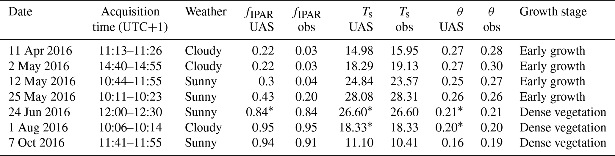
Due to technical issues, some UAS data from 24 June and 1 August were missing (Table 1), and in situ measurements were used to represent these missing values. For instance, to fill a prolonged gap in UAS observations in June of 2016 and to simulate the growth process of willow trees, in situ observations were added to 24 June. For model calibration, the instantaneous values of the T_s and θ estimated from the seven UAS flights were used as reference. The seven UAS flights resulted in an average flight frequency of 25 d for this growing season. The minimum revisit time was 10 d in the willow early growth period between 2 and 12 May. The maximum revisit time was 67 d between 1 August to 7 October when the willow canopy was dense and stable.

Figure 2 (a) Daily precipitation (P, mm d⁻¹), (b) daily air temperature (T_a, ^∘), and (c) daily fraction of the intercepted PAR (f_IPAR) interpolated from UAS-based NDVI during the 2016 growing season.

3 Method

The SVEN model is an operational and parsimonious remote-sensing-based land surface modelling scheme that expands the capabilities of the remote sensing GPP and Priestley–Taylor Jet Propulsion Laboratory (PT-JPL) ET model (Wang et al., 2018a) to be dynamic. It runs at half-hourly time steps and can temporally interpolate the instantaneous land surface variables, such as T_s, R_n, θ, ET, and GPP, into continuous records.

3.1 Model description

SVEN consists of a surface energy balance module, a water balance module, and a CO₂ flux module. In the energy balance module, SVEN estimates the surface temperature and ground heat flux, relying on the land surface energy balance equations and the “force-restore” method (Noilhan and Mahfouf, 1996; Noilhan and Planton, 1989) to consider the energy exchange between the ground and soil/vegetation on the surface. The water balance module includes the PT-JPL model for ET estimation and a simple “bucket” model representing the upper soil column to simulate soil water dynamics and runoff generation. The CO₂ flux module uses a light use efficiency (LUE) model for GPP estimation, which is connected to ET via the same canopy biophysical constraints. Figure 3 shows the major processes simulated in SVEN. Detailed information on these three modules is outlined below.

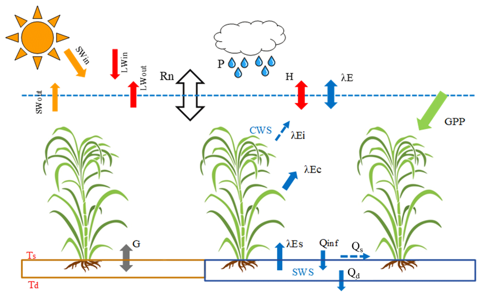
Figure 3 Major land surface processes simulated in SVEN. These processes include the land surface energy balance, water fluxes, and CO₂ assimilation. The abbreviations used in the figure are as follows: SW_in – incoming shortwave radiation; SW_out – outgoing shortwave radiation; LW_in – incoming longwave radiation; LW_out – outgoing longwave radiation; R_n – net radiation; G – ground heat flux; T_s – the surface temperature; T_d – the deep soil temperature; H – sensible heat flux; P – precipitation; λE – latent heat flux; λE_i – latent heat flux of the intercepted water; λE_c – latent heat flux of transpiration; λE_s – latent heat flux of soil evaporation; CWS – canopy water storage; SWS – soil water storage; Q_inf – infiltration; Q_d – drainage; Q_s – surface runoff; GPP – gross primary productivity.

3.1.1 Surface energy balance module

The instantaneous net radiation is estimated based on the surface energy balance, as shown in Eq. (1). The surface emissivity is approximated according to an empirical relation with the NDVI, as seen in Eq. (2) (Van de Griend and Owe, 1993). The surface albedo (A) is estimated from the simple ratio vegetation index (SR), and it shows that albedo generally decreases as vegetation greenness increases, as shown in Eqs. (3) and (4) (Gao, 1995).

$$\begin{array}{}\text{(1)}& {\displaystyle }& {\displaystyle }{R}_{\mathrm{n}}=(\mathrm{1}-A){\mathrm{SW}}_{\mathrm{in}}+(\mathrm{1}-\mathit{\epsilon }){\mathrm{LW}}_{\mathrm{in}}-\mathit{\epsilon }\mathit{\sigma }{T}_{\mathrm{s}}^{\mathrm{4}}\text{(2)}& {\displaystyle }& {\displaystyle }\mathit{\epsilon }=\left\{\begin{array}{ll}\mathrm{0.986}& (\mathrm{NDVI}>\mathrm{0.608})\\ \mathrm{1.0094}+\mathrm{0.047}\cdot \ln \left(\mathrm{NDVI}\right)& (\mathrm{0.131}<\mathrm{NDVI}<\mathrm{0.608})\\ \mathrm{0.914}& (\mathrm{NDVI}<\mathrm{0.131})\end{array}\right.\text{(3)}& {\displaystyle }& {\displaystyle }A=\mathrm{0.28}-\mathrm{0.14}{e}^{(-\mathrm{6.08}/{\mathrm{SR}}^{\mathrm{2}})}\text{(4)}& {\displaystyle }& {\displaystyle }\mathrm{SR}=(\mathrm{1}+\mathrm{NDVI})/(\mathrm{1}-\mathrm{NDVI})\end{array}$$

Here, Rn is the instantaneous net radiation (W m⁻²), SW_in is the instantaneous incoming shortwave radiation (W m⁻²), LW_in is the instantaneous incoming longwave radiation (W m⁻²), and σ is the Stefan–Boltzmann constant ($\mathrm{5.670367}\times {\mathrm{10}}^{-\mathrm{8}}$ W m⁻² K⁻⁴).

At the surface, R_n is dissipated as latent, sensible, and ground heat fluxes, as shown in Eq. (5). The latent heat flux is estimated from the PT-JPL ET model, and the sensible heat flux (H) is calculated based on the temperature gradient between the surface and air and a bulk aerodynamic resistance. The instantaneous ground heat flux (G) is estimated from the “force-restore” method (Noilhan and Planton, 1989).

$$\begin{array}{}\text{(5)}& {\displaystyle \frac{\mathrm{d}S}{\mathrm{d}t}}={\mathrm{SW}}_{\mathrm{in}}-{\mathrm{SW}}_{\mathrm{out}}+{\mathrm{LW}}_{\mathrm{in}}-{\mathrm{LW}}_{\mathrm{out}}-H-\mathit{\lambda }E-G,\end{array}$$

where $\frac{\mathrm{d}S}{\mathrm{d}t}$ is the heat storage change over time (W m⁻²), SW is shortwave radiation (W m⁻²), LW is longwave radiation (W m⁻²), the subscripts _in and _out refer to incoming and outgoing respectively, λE represents the latent heat flux (W m⁻²), H refers to the sensible heat flux (W m⁻²), and G is the ground heat flux (W m⁻²).

The surface temperature was estimated using the “force-restore” method, which considers two opposite effects on surface temperature variabilities, as shown in Eq. (6). The first term ($R_{\mathrm{n}}-\mathit{\lambda }E-H$) represents the forcing from the surface–atmosphere interface. The second term (T_s−T_d) is the gradient between the surface temperature and the deep soil temperature; it indicates the tendency of the deep soil to restore T_s (responding to surface energy forcing) to the T_d value, which is more stable over time.

$$\begin{array}{}\text{(6)}& {\displaystyle }& {\displaystyle \frac{\mathrm{d}{T}_{\mathrm{s}}}{\mathrm{d}t}}=C_{\mathrm{T}}\left(R_{\mathrm{n}}-\mathit{\lambda }E-H\right)-C_{\mathrm{d}}\left(T_{\mathrm{s}}-T_{\mathrm{d}}\right)\text{(7)}& {\displaystyle }& {\displaystyle \frac{\mathrm{d}{T}_{\mathrm{d}}}{\mathrm{d}t}}=\mathit{\omega }\left(T_{\mathrm{s}}-T_{\mathrm{d}}\right)\text{(8)}& {\displaystyle }& {\displaystyle \frac{\mathrm{1}}{C_{\mathrm{T}}}}={\displaystyle \frac{\mathrm{1}-f_{\mathrm{c}}}{C_{\mathrm{sat}}{\left(\frac{{\mathrm{SWS}}_{\max }}{\mathrm{SWS}}\right)}^{\frac{b}{\mathrm{2}\ln \left(\mathrm{10}\right)}}}}+{\displaystyle \frac{f_{\mathrm{c}}}{C_{\mathrm{veg}}}}\text{(9)}& {\displaystyle }& {\displaystyle }{C}_{\mathrm{d}}=\mathrm{2}\mathit{\pi }\mathit{\omega }\end{array}$$

Here, T_s is the land surface temperature (^∘C), T_d refers to the deep soil temperature (^∘C) calculated by applying a low-pass filter to T_s with a cut-off frequency of 24 h, ω is the frequency of oscillation 1∕24 (h⁻¹), C_T is a force-restore thermal coefficient for the surface heat transfer (K m² J⁻¹) and is influenced by the effective relative θ, C_sat is the force-restore thermal coefficient for saturated soil (K m² J⁻¹), the parameter b is the slope of the retention curve for the force-restore thermal coefficient, C_veg is the force-restore thermal coefficient for vegetation (K m² J⁻¹), f_c is the fractional cover of vegetation and is assumed to be equal to f_IPAR (as shown in Table S1 in the Supplement; Fisher et al., 2008), SWS_max is the maximum soil water storage (m), SWS is the actual soil water storage (m), and C_d is diurnal periodicity based on ω (h⁻¹).

The sensible heat flux (H) is estimated based on the temperature gradient between the surface and air:

$$\begin{array}{}\text{(10)}& H=\mathit{\rho }{c}_{\mathrm{p}}\left(T_{\mathrm{s}}-T_{\mathrm{a}}\right)/r_{\mathrm{a}},\end{array}$$

where ρ is the air density (kg m⁻³), c_p is the specific heat capacity of air (J kg⁻¹ K⁻¹), T_s is the land surface temperature (^∘C), T_a is the air temperature (^∘C), and r_a is the aerodynamic resistance for heat transfer (s m⁻¹).

Aerodynamic resistance to turbulent transport under neutral conditions (r_aN) can be expressed as follows (Brutsaert, 1982):

$$\begin{array}{}\text{(11)}& {\displaystyle }& {\displaystyle }{r}_{\mathrm{aN}}={\displaystyle \frac{\ln \left(\frac{z-d}{z_{\mathrm{om}}}\right)\ln \left(\frac{z-d}{z_{\mathrm{oh}}}\right)}{k^{\mathrm{2}}u}}\text{(12)}& {\displaystyle }& {\displaystyle }d=\mathrm{0.67}{h}_{\mathrm{c}}\text{(13)}& {\displaystyle }& {\displaystyle }{z}_{\mathrm{om}}=\mathrm{0.1}{h}_{\mathrm{c}}\text{(14)}& {\displaystyle }& {\displaystyle }{z}_{\mathrm{oh}}={\displaystyle \frac{z_{\mathrm{om}}}{e^{k{B}^{-\mathrm{1}}}}},\end{array}$$

where h_c is the canopy height (m), the parameter d is the zero displacement height (m), z is the velocity reference height (m), z_om is the aerodynamic roughness length for momentum (m), z_oh is the aerodynamic roughness length for the heat transfer (m), u is the horizontal wind velocity at a reference height (m s⁻¹), kB⁻¹ is a parameter to account for the difference between the aerodynamic and radiometric temperatures – a constant value of 2.3 is adopted in this study (Garratt and Hicks, 1973), and k is the von Karman constant (0.4).

The aerodynamic resistance is corrected for the atmospheric stability as shown in Eq. (15) (Huning and Margulis, 2015), where Ψ_m is the stability correction factor for momentum, and Ψ_h is the stability correction factor for sensible heat flux. For unstable conditions (negative temperature gradient), the stability correction factors are less than 1.0, and the correction reduces the resistance and enhances turbulence; for stable conditions, they are greater than 1.0, and the correction increases the resistance and suppresses turbulence.

$$\begin{array}{}\text{(15)}& r_{\mathrm{a}}=r_{\mathrm{aN}}{\mathrm{\Psi }}_{\mathrm{m}}{\mathrm{\Psi }}_{\mathrm{h}}\end{array}$$

When the atmospheric condition is unstable (R_iB≤0), Ψ_m and Ψ_h are estimated as follows:

$$\begin{array}{}\text{(16)}& {\mathrm{\Psi }}_{\mathrm{h}}={\mathrm{\Psi }}_{\mathrm{m}}^{\mathrm{2}}={\left(\mathrm{1}-\mathrm{15}{R}_{\mathrm{iB}}\right)}^{-\mathrm{1}/\mathrm{2}}\end{array}$$

When the atmospheric condition is stable ($\mathrm{0}\le R_{\mathrm{iB}}<\mathrm{0.2}$), Ψ_m and Ψ_h are estimated as follows:

$$\begin{array}{}\text{(17)}& {\displaystyle }& {\displaystyle }{\mathrm{\Psi }}_{\mathrm{h}}={\mathrm{\Psi }}_{\mathrm{m}}={\left(\mathrm{1}-\mathrm{5}{R}_{\mathrm{iB}}\right)}^{-\mathrm{1}}\text{(18)}& {\displaystyle }& {\displaystyle }{R}_{\mathrm{iB}}={\displaystyle \frac{\left(\frac{g}{T_{\mathrm{s}}}\right)\partial T_{\mathrm{s}}/\partial z}{{\left(\frac{\partial u}{\partial z}\right)}^{\mathrm{2}}}}\end{array}$$

Here, R_iB is the bulk Richardson number, and g is the gravitational acceleration.

3.1.2 Water balance module

The water balance module simulates the evaporation of intercepted water, plant transpiration, soil evaporation, soil water infiltration, and drainage. The evapotranspiration is estimated based on a modified PT-JPL ET model (Wang et al., 2018a). The PT-JPL ET model has been demonstrated to be one of best performing global remote sensing ET algorithms (Chen et al., 2014; Ershadi et al., 2014; Miralles et al., 2016; Vinukollu et al., 2011). Thus, it was selected for ET estimation. The PT-JPL model (Fisher et al., 2008) uses the Priestley–Taylor (Priestley and Taylor, 1972) equation to calculate the potential evapotranspiration and then incorporates ecophysiological variables to down-regulate potential evapotranspiration to actual evapotranspiration. PT-JPL is a three-source evapotranspiration model to simulate the respective evaporation of intercepted water (E_i), transpiration (E_c), and soil evaporation (E_s) as follows:

$$\begin{array}{}\text{(19)}& {\displaystyle }& {\displaystyle }\mathit{\lambda }\mathrm{ET}=\mathit{\lambda }E-\mathrm{i}+\mathit{\lambda }{E}_{\mathrm{c}}+\mathit{\lambda }{E}_{\mathrm{s}}\text{(20)}& {\displaystyle }& {\displaystyle }\mathit{\lambda }{E}_{\mathrm{i}}=f_{\mathrm{wet}}\cdot \mathit{\alpha }\mathrm{\Delta }/(\mathrm{\Delta }+\mathit{\gamma })\cdot R_{\mathrm{nc}}\text{(21)}& {\displaystyle }& {\displaystyle }\mathit{\lambda }{E}_{\mathrm{c}}=\left(\mathrm{1}-f_{\mathrm{wet}}\right)\cdot f_{\mathrm{g}}\cdot f_{\mathrm{M}}\cdot f_{T_{\mathrm{a}}}\cdot {\mathit{\alpha }}_{\mathrm{c}}\mathrm{\Delta }/(\mathrm{\Delta }+\mathit{\gamma })\cdot R_{\mathrm{nc}}\text{(22)}& {\displaystyle }& {\displaystyle }\mathit{\lambda }{E}_{\mathrm{s}}=f_{\mathit{\theta }}\cdot \mathit{\alpha }\mathrm{\Delta }/(\mathrm{\Delta }+\mathit{\gamma })\cdot \left(R_{\mathrm{ns}}-G\right)\end{array}$$

Here, λET is the latent heat flux for total evapotranspiration (W m⁻²), λE_i is the latent heat flux due to the evaporation of intercepted water (W m⁻²), λE_c is the latent heat flux due to transpiration (W m⁻²), and λE_s is the latent heat flux due to evaporation of soil water (W m⁻²). The quantity f_wet is the relative surface wetness to partition the evapotranspiration from the intercepted water and canopy transpiration, f_g is the green canopy fraction indicating the proportion of active canopy, f_M is the plant moisture constraint, $f_{T_{\mathrm{a}}}$ is the plant temperature constraint reflecting the temperature limitation of photosynthesis, and f_θ is the θ constraint. These constraints vary from zero to one to account for the relative reduction of potential λET under limiting environmental conditions. R_nc and R_ns are the net radiation for canopy and soil respectively. The partitioning of PAR and net radiation between the canopy and soil is calculated following the Beer–Lambert law (Table S1). G is the ground heat flux. Δ is the slope of the saturation vapour pressure versus the temperature curve. γ is the psychrometric constant. α is an empirical ratio of potential evapotranspiration to equilibrium potential evapotranspiration (the Priestley–Taylor coefficient); the suggested value for α is 1.26 in the PT-JPL model (Fisher et al., 2008).

In the original model, f_wet was estimated from air relative humidity (Fisher et al., 2008). In this study, f_wet is modified to be defined as a ratio between the actual canopy water storage (CWS) and the maximum canopy water storage (CWS_max), as shown in Eq. (23) (Noilhan and Planton, 1989). CWS is the amount of intercepted water, and CWS_max is the maximum possible amount of intercepted water (mm), which is taken as 0.2 LAI kg m⁻² (Dickinson, 1984). f_wet depends on both the precipitation rate and LAI, which is more reasonable than only depending on air relative humidity in the original model.

$$\begin{array}{}\text{(23)}& f_{\mathrm{wet}}={\displaystyle \frac{\mathrm{CWS}}{{\mathrm{CWS}}_{\max }}}\end{array}$$

In this study, we determined CWS using a prognostic equation (Eq. 24) with the constraint that CWS is smaller than CWS_max.

$$\begin{array}{}\text{(24)}& {\displaystyle \frac{\mathrm{dCWS}}{\mathrm{d}t}}=f_{\mathrm{c}}\cdot P-E_{\mathrm{i}},\end{array}$$

where f_c is the fraction of vegetation cover, which is assumed to be equal to f_IPAR in this study (Fisher et al., 2008). P and E_i are the rainfall rates and the evaporation from the intercepted water respectively (m s⁻¹).

The effective precipitation rate is estimated as the residual of the rainfall rate and the change in CWS:

$$\begin{array}{}\text{(25)}& P_{\mathrm{e}}=P-\mathrm{dCWS}\end{array}$$

To simulate the dynamics of water storage in the soil, SVEN uses a simple bucket model. Here, the infiltration rate (Q_inf) is equal to the effective rainfall rate (P_e), when the soil water is not saturated. Thus, SWS is calculated based on a prognostic equation with the constraint that SWS is smaller than SWS_max.

$$\begin{array}{}\text{(26)}& {\displaystyle }& {\displaystyle }{Q}_{\inf }=P_{\mathrm{e}}\text{(27)}& {\displaystyle }& {\displaystyle \frac{\mathrm{dSWS}}{\mathrm{d}t}}=Q_{\inf }-E_{\mathrm{c}}-E_{\mathrm{s}}-Q_{\mathrm{d}}\end{array}$$

When the soil water is saturated, SWS is equal to SWS_max, and surface runoff (Q_s) occurs, as shown in Eq. (29).

$$\begin{array}{}\text{(28)}& {\displaystyle }& {\displaystyle }{Q}_{\inf }=E_{\mathrm{c}}+E_{\mathrm{s}}+Q_{\mathrm{d}}\text{(29)}& {\displaystyle }& {\displaystyle }{Q}_{\mathrm{s}}=P_{\mathrm{e}}-Q_{\inf }\end{array}$$

Here, SWS is soil water storage (m), and P_e, E_c, E_s, Q_d, and Q_s are the effective rainfall rates, transpiration rates, evapotranspiration rates from soil, drainage rates, and surface runoff (m s⁻¹) respectively.

Soil water drainage, which is leakage out of the lower boundary of the flow domain (Romano et al., 2011), is computed by assuming the condition of a unit gradient of the total hydraulic potential at the lowest boundary and using the van Genuchten (1980) soil–water retention relationship:

$$\begin{array}{}\text{(30)}& {\displaystyle }& {\displaystyle }{Q}_{\mathrm{d}}=K_{\mathrm{s}}\sqrt{{\mathit{\theta }}_{\mathrm{e}}}{\left(\mathrm{1}-{\left(\mathrm{1}-{\mathit{\theta }}_{\mathrm{e}}^{\mathrm{1}/(\mathrm{1}-\mathrm{1}/n)}\right)}^{\mathrm{1}-\mathrm{1}/n}\right)}^{\mathrm{2}}\text{(31)}& {\displaystyle }& {\displaystyle }{\mathit{\theta }}_{\mathrm{e}}={\displaystyle \frac{\mathit{\theta }-{\mathit{\theta }}_{\mathrm{r}}}{{\mathit{\theta }}_{\mathrm{s}}-{\mathit{\theta }}_{\mathrm{r}}}},\end{array}$$

where K_s is the saturated hydraulic conductivity (m s⁻¹), n is the shape parameter of the van Genuchen (1980) soil–water retention relationship and depends on the pore-size distribution, θ is the volumetric soil moisture (m³ m⁻³), θ_e is the effective soil moisture (m³ m⁻³), θ_s is the saturated soil moisture (m³ m⁻³), and θ_r is the residual soil moisture (m³ m⁻³).

3.1.3 CO₂ flux module

The photosynthesis in the CO₂ flux module is calculated from a modified light use efficiency (LUE) model (Wang et al., 2018a) linked to the biophysical constraints for canopy transpiration of the PT-JPL model. The LUE GPP model is a robust and widely used method to estimate GPP across various ecosystems and climate regimes (McCallum et al., 2009). The LUE models, e.g. the Carnegie Ames Stanford Approach model (CASA; Potter et al., 1993) or the MODIS algorithm (Running et al., 2004), are based on the assumption that plants optimize canopy LUE or whole canopy carbon gain per total PAR absorbed as originally suggested by Monteith (1972) for net primary productivity. The formula of the LUE GPP model used in this study is shown in Eq. (32), and it is partly based on the CASA model (Potter et al., 1993) with a modification to include an additional constraint accounting for the fraction of the canopy that is photosynthetically active (Fisher et al., 2008). Other constraints such as thermal regulation (Wang et al., 2018a) reflect changes in the LUE due to environmental factors and are the same for regulating ET_c (Eq. 21).

$$\begin{array}{}\text{(32)}& \mathrm{GPP}={\mathrm{LUE}}_{\max }\cdot {\mathrm{PAR}}_{\mathrm{c}}\cdot f_{\mathrm{g}}\cdot f_{\mathrm{M}}\cdot f_{T_{\mathrm{a}}}\cdot f_{\mathrm{VPD}},\end{array}$$

where LUE_max is the maximum LUE (g C MJ⁻¹); PAR_c is the daily photosynthetically active radiation (PAR) (MJ m⁻² d⁻¹) intercepted by the canopy, and it is calculated based on the extinction of PAR within the canopy using the Beer–Lambert law (Table S1); f_g is the green canopy fraction indicating the proportion of active canopy; f_M is the plant moisture constraint; $f_{T_{\mathrm{a}}}$ is the air temperature constraint reflecting the temperature limitation of photosynthesis; and f_VPD is the VPD constraint reflecting the stomatal response to the atmospheric water saturation deficit. All of these constraints range from zero and one and represent the reduction in the maximum GPP under limiting environmental conditions. For more details, please refer to the Table S1.

3.2 Model implementation

The SVEN model requires shortwave incoming (SW_in) radiation, longwave incoming (LW_in) radiation, air temperature (T_a), air pressure (P_s), relative humidity (RH), wind speed (u), precipitation (P), canopy height (z), and vegetation information (NDVI) as inputs (Table S2). The model inputs of this study were obtained from meteorological data, UAS-derived observations, or estimates. The simulation outputs of this model are shown in Table S4. The initial conditions for the model include an initial canopy water storage (CWS_in), an initial soil water storage (SWS_in), initial surface temperature ($T_{{\mathrm{s}}_{\mathrm{0}}}$), and initial deep soil temperature ($T_{{\mathrm{d}}_{\mathrm{0}}}$), as shown in Table S3. The initial conditions to run the model (11 April to 7 October 2016) were obtained by performing spin-up simulations from 11 March to 11 April 2016. The details of model implementation are shown in Fig. 4.

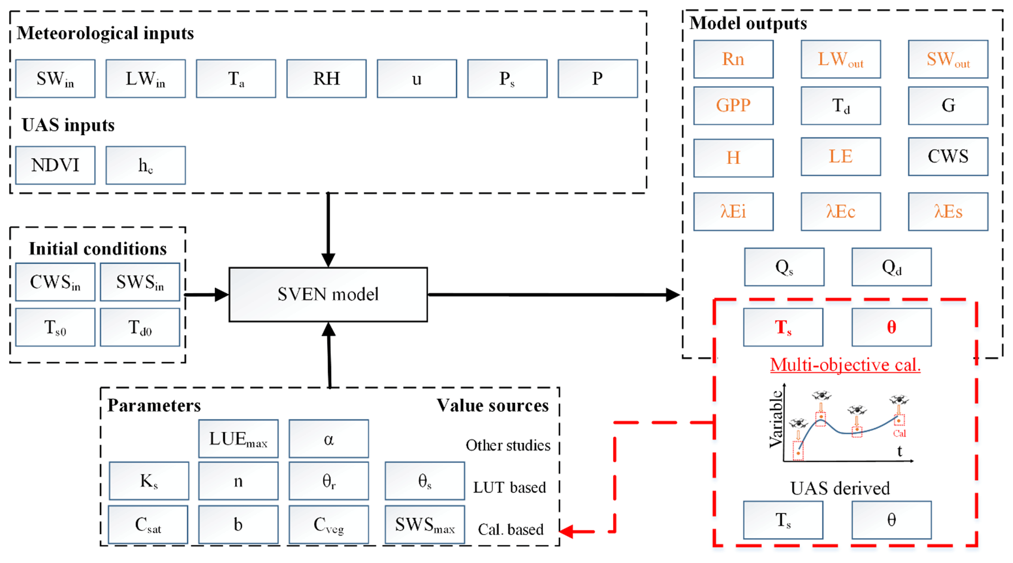
Figure 4 Model implementation in this study. UAS and meteorological data were used as inputs for the SVEN model. Values of the SVEN parameters were obtained from other studies, look-up tables (LUT based), or model calibration with UAS-derived variables (Cal. based). In the model outputs, variables written in red (T_s and θ) refer to the variables calibrated with UAS-derived observations or estimates. The red shaded box represents the multi-objective calibration process with UAS-derived T_s and θ. The variables written in orange are retrievable using remote sensing techniques.

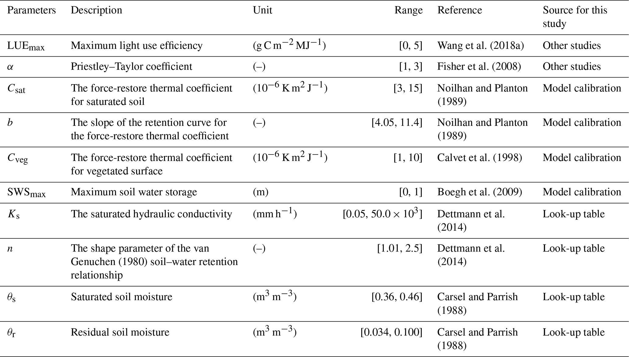
The SVEN model has six parameters that are mostly related to physical soil properties for heat transfer and infiltration (Table 2). The parameter values can be obtained using multiple approaches, including look-up tables based on soil texture, parameter values from similar biome or soil types from other studies, field measurements, or model parameter optimization with in situ measurements or remote sensing data. This study used a combination of these approaches to obtain model parameter values (Fig. 4). The parameters, such as the maximum light use efficiency (LUE_max), that were used to drive the snapshot version of SVEN were obtained from a nearby similar deciduous temperate forest ecosystem (Wang et al., 2018a). The shape parameter of the van Genuchen (1980) soil–water retention relationship (n) and the saturated hydraulic conductivity (K_s) were obtained from a look-up table (Carsel and Parrish, 1988). The values for loamy soil shown in the Table S5 were used, and they were based on the soil texture of this site. The rest of the parameters related to the soil and vegetation physical properties (C_sat, b, C_veg and SWS_max) were obtained by calibrating models using instantaneous T_s and θ from seven UAS flight campaigns (Table 1) rather than via calibration with in situ measurements of ET or GPP (e.g. eddy covariance data) as in other studies. Calibrating the model with the remotely-sensed instantaneous estimates instead of ground measurements facilitates the application of this approach in data-scarce regions. The calibration of C_sat, b, C_veg, and SWS_max was conducted using the Monte Carlo optimization. The parameter values were sampled 20 000 times with a uniform distribution and the corresponding parameter ranges (as shown in Table 2). The objective function for optimization is the root mean square deviation (RMSD) between the observed and simulated values. With two objective functions for T_s and θ respectively, the multiple objective optimization method (Pareto front; as show in Yapo et al., 1998) was used to identify the optimized parameter values.

Table 2 Information on the model parameters of SVEN and their ranges for all soil or biome types.

3.3 Model assessment

We used independent eddy covariance data to validate model outputs. However, due to the energy balance closure issue (Wilson et al., 2002), the sum of sensible heat (H) and latent heat (LE) as measured by the eddy covariance method is generally not equal to the available energy (net radiation minus ground heat flux, R_n−G). This study used the Bowen ratio approach to correct energy balance closure errors of eddy covariance data. Using the ratio of 30 min sensible heat to ET (Bowen ratio), LE measurements can be corrected as follows (Twine et al., 2000). LE data with a 30 min energy balance closure error larger than 20 % were excluded from the validation.

$$\begin{array}{}\text{(33)}& LE={\displaystyle \frac{R_{\mathrm{n}}-G}{\mathrm{H}\mathrm{\_}\mathrm{EC}\mathrm{\_}\mathrm{raw}+\mathrm{LE}\mathrm{\_}\mathrm{EC}\mathrm{\_}\mathrm{raw}}}\mathrm{LE}\mathrm{\_}\mathrm{EC}\mathrm{\_}\mathrm{raw},\end{array}$$

where LE is corrected latent heat by assuming the constant Bowen ratio (W m⁻²), R_n is net radiation (W m⁻²), G is ground heat flux (W m⁻²), H_EC_raw is uncorrected sensible heat (W m⁻²), and LE_EC_raw is uncorrected latent heat (W m⁻²).

The SVEN model was developed to interpolate between remote sensing data acquisitions and to produce continuous daily records. Thus, the observed T_s, R_n, LE, and GPP are from the eddy covariance system, and the in situ θ measurements at a depth of 15 cm (sensor location in Fig. 1) were used to validate the simulated variables at a daily timescale. Statistics including the RMSD, the coefficient of determination (R²), relative errors (RE), the and normalized RMSD (NRMSD – the ratio between RMSD and the range of observations) were used in validation.

We also analysed how the model skill changed depending on vegetation cover and overcast (diffuse radiation) conditions by looking at model residuals; this is due to the fact that remote sensing models are typically biased to sunny conditions. Scatterplots between model residuals and the NDVI and the diffuse radiation fraction were examined. As the ratio between the actual (SW_in) and potential (SW_in,pot) solar radiation can be an indicator of the diffuse radiation fraction (Wang et al., 2018a), we used this ratio to indicate the diffuse radiation fraction. This analysis can help to understand possible methods to improve the SVEN model. To check the capability of the SVEN model to interpolate half-hourly and monthly time series fluxes, the simulated land surface variables were also validated at half-hourly and monthly timescales, in addition to the daily timescale.

4 Results and discussion

4.1 Model parameter estimation

Figure 5 illustrates the results of model parameter calibration with UAS-derived snapshot θ and T_s (Table 1). With RMSD values of θ and T_s as objective functions, a significant trade-off between the performance of θ and T_s simulations is observed as a Pareto front (the red curve) in Fig. 4. The x axis shows the performance of simulating θ. The smaller the RMSD values are, the better the model performance with respect to this variable. The minimum, however, lies in a range where the model performance of the other variable, T_s, is highest (y axis). From the viewpoint of multi-objective optimization, the solutions at the Pareto front are equally good. By considering RMSD values of T_s that are less than 2 ^∘C and RMSD values of θ that are as small as possible, we selected the point close to the red arrow in Fig. 4, which corresponds to the RMSD values of θ and T_s that are equal to 2.99 % m³ m⁻³ and 1.92 ^∘C respectively. The values of C_sat, b, C_veg, and SWS_max at this Pareto-front point are equal to $\mathrm{6.94}\times {\mathrm{10}}^{-\mathrm{6}}$ K m² J⁻¹, 5.20, $\mathrm{2.18}\times {\mathrm{10}}^{-\mathrm{6}}$ K m² J⁻¹, and $\mathrm{5.54}\times {\mathrm{10}}^{-\mathrm{1}}$ m respectively. Furthermore, we also analysed the variability of optimized parameter values, as shown in Fig. S1 in the Supplement. C_veg and SWS_max show low coefficients of variation (CVs), and this indicates the parsimony of the SVEN model. Meanwhile, C_sat and b show relatively higher CVs. This may be due to equifinality between C_sat and b, which relate to soil thermal properties (Eq. 8) and could compensate for each other. Notably, these calibrated values, e.g. SWS_max, represents the equivalent calibrated parameter value and might be different from the actual physical conditions.

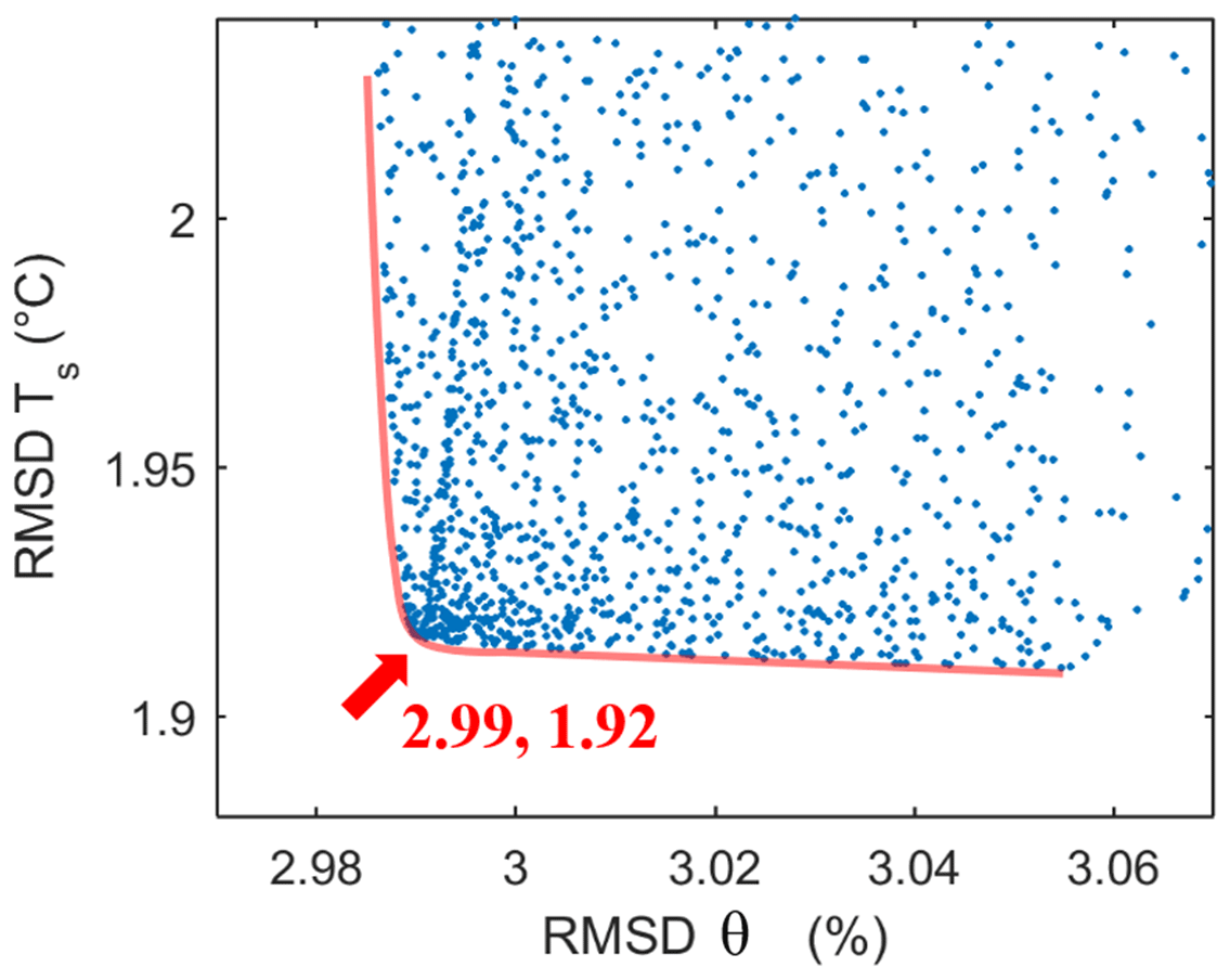
Figure 5 Objective function values of the evaluated parameter sets and the corresponding Pareto front. The x axis is the objective function for simulating θ; the y axis is the objective function for simulating T_s. Each dot corresponds to one simulation performance. Each of the simulations represents a different combination of candidate parameter sets. The dot closest to the red arrow was chosen to be the optimal parameter set for the SVEN continuous simulation. C_sat, b, C_veg, and SWS_max at the Pareto-front point are $\mathrm{6.94}\times {\mathrm{10}}^{-\mathrm{6}}$ K m² J⁻¹, 5.20, $\mathrm{2.18}\times {\mathrm{10}}^{-\mathrm{6}}$ K m² J⁻¹, and $\mathrm{5.54}\times {\mathrm{10}}^{-\mathrm{1}}$ m respectively.

4.2 Validation at the daily timescale

Figure 6 shows the time series data of the interpolated daily T_s, R_n, θ, LE, and GPP as well as their validation. The simulated daily T_s, R_n, θ, LE, and GPP capture the observed temporal dynamics of land surface variables at this site well. R² for daily T_s, R_n, θ, LE, and GPP are 0.90, 0.92, 0.50, 0.70, and 0.79 respectively. RMSD values for the simulated daily T_s, R_n, θ, LE, and GPP are 2.35 ^∘C, 14.49 W m⁻², 1.98 % m³ m⁻³, 16.62 W m⁻², and 3.01 g C m⁻² d⁻¹ respectively. Such simulation accuracy demonstrates that SVEN is capable of temporally interpolating the snapshot estimates or observations between remote sensing acquisitions to form continuous daily records.

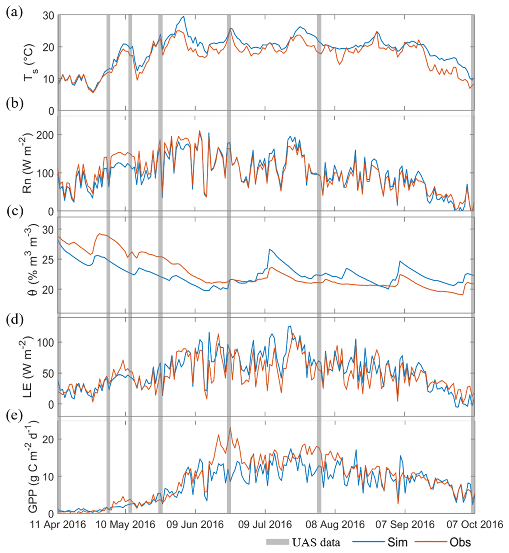
Figure 6 Simulated continuous daily land surface variables from 11 April to 7 October 2016 at the willow plantation: (a) land surface temperature (T_s), (b) net radiation (R_n), (c) soil moisture(θ), (d) latent heat flux (LE), and (e) gross primary productivity (GPP). The grey shaded area indicates the time of acquired data for model calibration, and the blue and red curves represent simulations and observations respectively.

For the simulated T_s, during the early growth stage (before June), the SVEN model quite accurately simulated the temporal dynamics. However, during the dense vegetation stage (high NDVI), the model generally tended to overestimate T_s. Similarly, SVEN underestimated R_n during the early growth stage, but overestimated R_n for the dense vegetation stage. These biases can also be identified from the boxplots of model residuals and NDVI (Fig. 7b), which show that the model underestimates R_n under low NDVI conditions and vice versa. One of the reasons for this error could be the uncertainty in the estimated surface albedo. The albedo in the SVEN model was determined by the simple empirical formula shown in Eq. (3), with a high value in the early growth stage and a low value for dense vegetation. Another possible source of errors is uncertainties in C_veg, which reflects the thermal storage property of vegetated surface in the force-restore method. C_veg was obtained via model calibration with UAS-observed T_s. As shown in Fig. 2, only three UAS data sets were available for the vegetated period. Therefore, the insufficient model calibration may lead to uncertainties in C_veg.

Figure 7 Boxplots of the residuals for the daily simulation. Panels (a–e) show the simulation residuals and NDVI. Panels (f–j) show simulation residuals and the ratio of the actual (SW_in) and potential (SW_in,pot) solar radiation, which is an indicator of the cloudiness condition. Panels (a) and (f) show the surface temperature (T_s); (b) and (g) show the net radiation (R_n); (c) and (h) show the soil moisture (θ); (d) and (i) show the latent heat flux (LE); and (e) and (j) show the gross primary productivity (GPP). The blue dashed lines refer to the zero residuals.

The estimated θ from SVEN achieved moderate performance in terms of errors and correlation. The model underestimates θ when the NDVI is low, but it overestimates θ when the NDVI is high, as shown in Fig. 7c. Such errors may be due to the uncertainty in the model parameters related to θ. As shown in Table S5, the effective parameter values of K_s and n were taken as the mean values from the look-up table without considering the ranges of variability (standard deviations in the table). In fact, only one parameter, SWS_max, among the three parameters related to θ dynamics was calibrated with UAS estimates of θ in the root zone. To keep the model simple and parsimonious, the SVEN model only used one soil layer to simulate the dynamics of soil water storage (Fig. 3). Similarly, the model also assumed that the residual soil moisture is equal to the soil wilting points. In the simulation of runoff generation, this simple model only considered the dominant runoff process, the “Dunne” mechanism (runoff occurs after soil water saturation; Dunne and Black, 1970) instead of the “Hortonian” mechanism (runoff occurs when rainfall intensity exceeds the infiltration capacity; Horton, 1933), for this humid and flat site. Such model simplification could contribute to the relatively moderate performance of simulating θ. Additionally, UAS-derived θ estimates used for calibration have errors of around 13 % compared with the direct measurements (Wang et al., 2018a), which can induce uncertainties in the simulated time series due to error propagation in the parameter calibration. Furthermore, only seven snapshot estimates from the UAS were used to calibrate the model with an average frequency of 25 d during the period of fast growth. It can be expected that improving the UAS-based estimates of θ, increasing the number of observations for model calibration, and adding more complexity to the model structure will improve simulation performance. For instance, when applying SVEN to other regions, the “Dunne” or “Hortonian” mechanism needs to be selected to simulate the surface water processes, according to the soil, vegetation, and topographic conditions (Tauro et al., 2016).

The results of the simulated LE and GPP are shown in Fig. 6d and e respectively. In most cases, the simulation shows the overestimation of LE, which closely relates to the estimates of R_n and θ. The simulation underestimated GPP, as the LUE_max parameter was assumed to be the same as that from a nearby beech forest (Wang et al., 2018a). Even though both sites are temperate deciduous forests, differences still exist between the natural beech forest and the willow forest bioenergy plantation. Notably, there is a significant underestimation of the simulated GPP in June 2016, as shown in Fig. 6e. Besides the possible uncertainties from the LUE_max described above, the underestimation may also result from the observation uncertainties in the partitioning of the GPP and respiration in the eddy covariance data processing. In data processing, the night-time net ecosystem exchanges were used to calculate the ecosystem respiration. During the night-time, the eddy covariance footprint extended well beyond the edges of the willow forest of interest due to the stable atmospheric conditions. The tillage practices in the nearby rapeseed fields (Fig. 1) could contribute to the overestimation of daytime ecosystem respiration which, in turn, leads to the overestimation of the GPP in the eddy covariance data processing.

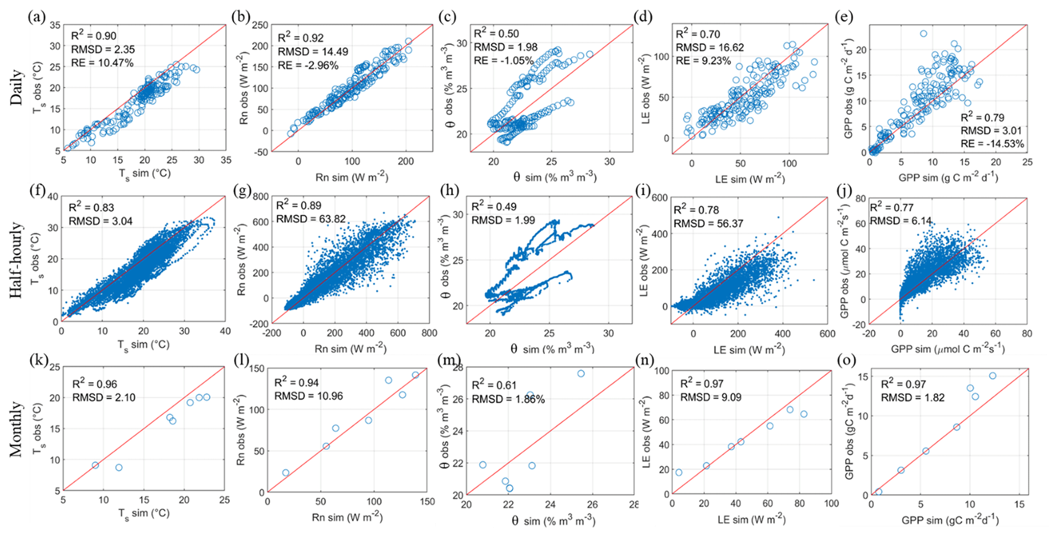
Figure 8 Validation of the interpolated land surface variables at daily, half-hourly, and monthly timescales at the willow plantation: panels (a–e) show the daily scale, (f–j) show the half-hourly scale, and (k–o) show the monthly scale. Panels (a), (f), and (k) show the surface temperature (T_s); (b), (g), and (l) show the net radiation (R_n); (c), (h), and (m) show the soil moisture (θ); (d), (i), and (m) show the latent heat flux (LE); and (e), (j), and (o) show the gross primary productivity (GPP). The RE metrics for the half-hourly and monthly scales are not shown, as they are the same as the RE at the daily scale.

To check the model simulation performance under cloudy conditions, we analysed the relationship between the model residuals and the ratio representing the diffuse radiation fraction (Fig. 7f–j). There were no significant differences for the residuals of the simulated T_s, R_n, θ, LE, and GPP under low and high diffuse radiation fraction conditions. Due to the ability of the UAS to acquire data under both cloud cover and clear-sky conditions, the SVEN model was capable of interpolating land surface variables under cloud cover conditions with a similar skill as under clear-sky conditions.

4.3 Validation at half-hourly and monthly timescales

Validation of the half-hourly and monthly T_s, R_n, θ, LE, and GPP by the SVEN model is shown in Fig. 8. The simulated half-hourly T_s, R_n, θ, LE, and GPP captured the temporal dynamics of land surface fluxes at this site. RMSD values for half-hourly T_s, R_n, θ, LE, and GPP are 3.04 ^∘C, 63.82 W m⁻², 1.99 % m³ m⁻³, 56.37 W m⁻², and 6.14 µmol C m⁻² s⁻¹ respectively. Compared with the simulation performance at the daily timescale (as shown in Table 3), the half-hourly simulation has higher RMSDs and lower R² values. Such performance may be due to the fact that parts of the SVEN modules are more suitable for daily-scale simulation instead of half-hourly-scale simulation. For instance, the simulation of LE in SVEN is based on the Priestley–Taylor equation that was originally applied to estimate monthly LE (Fisher et al., 2008) and was extended to be applied at daily steps (García et al., 2013); however, it is not appropriate to represent LE processes at sub-daily timescales.

Table 3 Comparison of model simulation performance at half-hourly, daily, and monthly timescales.

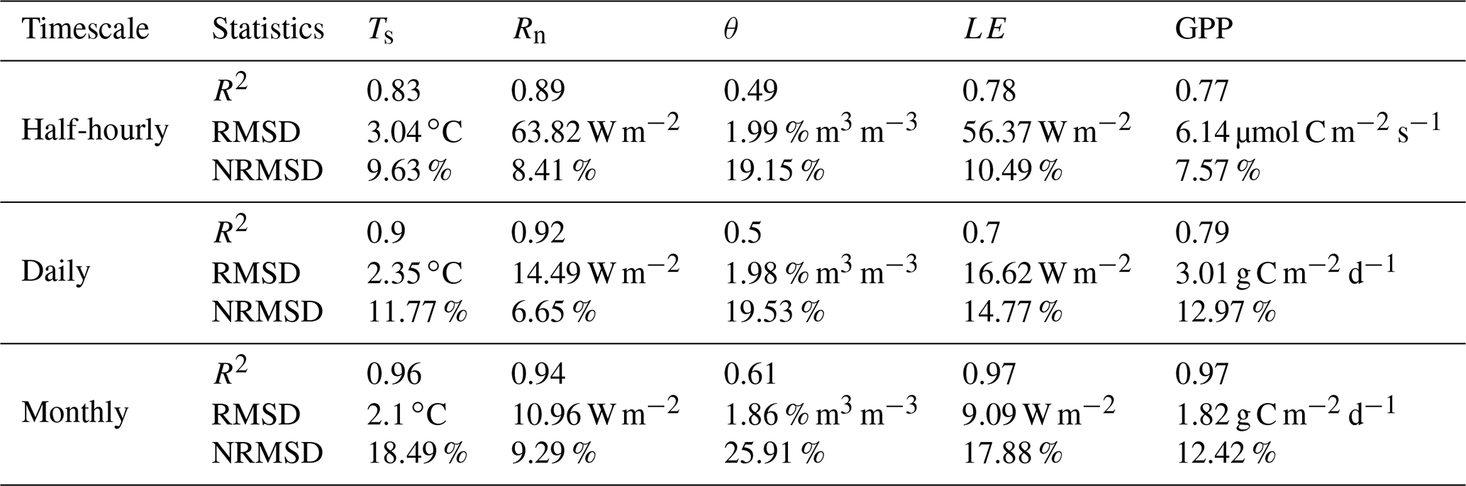
Regarding the monthly timescale, RMSDs for T_s, R_n, θ, LE, and GPP are 2.10 ^∘C, 10.96 W m⁻², 1.86 % m³ m⁻³, 9.09 W m⁻², and 1.82 g C m⁻² d⁻¹ respectively. The monthly simulation has lower RMSDs and slightly higher R² values compared with the daily simulation. The improvement of model performance from the half-hourly to the daily and monthly timescales indicates that the model errors can be reduced by aggregating the simulation outputs to longer timescales. Such accuracy also implies that the SVEN model has greater potential to temporally interpolate remote sensing observations at daily and monthly timescales, which are more relevant for applications in agriculture and ecosystem management.

4.4 Potential applications and improvement of SVEN

This study showed SVEN as a tool to temporally interpolate land surface variables between remote sensing acquisitions with few meteorological data. With respect to statistical approaches, Alfieri et al. (2017) identified that a return interval of remote sensing observations should be no less than 5 d to accurately interpolate daily ET with relative errors of less than 20 %. The results shown from our model-based interpolation approach in the willow forest suggest that the revisit time for remote sensing observations can potentially be extended. For instance, seven instantaneous observations/simulations of this study with an averaged revisit time of 25 d can accurately interpolate the daily ET for 180 d. This comparison shows the benefits of using the model-based approach to continuously estimate land surface fluxes from remote-sensing-based snapshot observations or estimates. The model-based approach can be used to estimate ecosystem states and flux exchange with the atmosphere for a landscape (e.g. crop fields) with temporally sparse UAS flight campaigns. This approach has great potential for agricultural ecosystem monitoring and management. The interpolated continuous record of land surface variables can also further facilitate our understanding of the temporal dynamics of land surface–atmosphere flux exchanges.

On the other hand, this study also provides ideas to utilize remote sensing estimates or observations to improve land surface modelling. Traditionally, the applicability of land surface models is limited due to complex model parameterization and the limited availability of “ground truth” or in situ data for parameter calibration. As shown in this study, one solution for this limitation is using remote-sensing-based observations or estimates as “ground truth” for model calibration (Stisen et al., 2011; Zhang et al., 2009). This study calibrated the model parameters through remote sensing snapshot (UAS) estimates of land surface variables such as T_s and θ and provided an example of integrating remote sensing data and process-based models. Other variables such as R_n, ET, and GPP, as shown in Fig. 4, could also be incorporated for model calibration. Compared with complex land surface models, this approach is simple and efficient and is especially suitable for operational applications to interpolate the remote-sensing-based snapshot estimates into the temporally continuous values.

Both the look-up table and parameter optimization approaches were used in this study to obtain the parameter values. For instance, we used a look-up table (Carsel and Parrish, 1988) to get values of n and K_s. The advantage of using the look-up table approach is that it can be easily applied according to the site conditions, such as vegetation types, soil texture and soil depth. However, this approach requires prior knowledge of the site. Insufficient knowledge of the site conditions may lead to the selection of unsuitable parameter values from the look-up tables. For instance, K_s may vary in different soil layers, and it could be difficult to select an effective K_s value to represent the condition of all of the soil layers. Regarding the optimization approach, this method has the advantage of achieving good fitting performance with UAS-derived observations or estimates. However, this approach needs to consider the number of observations and calibration parameters, parameter equifinality, and multi-objective optimization (Her and Chaubey, 2015). For instance, due to the limited number (14) of UAS-derived T_s or θ values available for calibration, we only selected four parameters (C_sat, b, C_veg, and SWS_max), which are hard to obtain from the look-up table approach with insufficient prior knowledge of the site, for optimization. To deal with parameter equifinality and multi-objective optimization, the Monte Carlo optimization was combined with the Pareto-front analysis in this study. Other approaches, e.g. Bayesian analysis, could also be utilized to calibrate the model parameter with multiple objectives and separate the uncertainty sources, including input, parameters, and model structure, to quantify the simulated uncertainties (Vrugt et al., 2009). Besides the look-up table and optimization approaches, another promising approach is the estimation of soil or plant hydraulic properties from imaging spectroscopy (Goldshleger et al., 2012; Nocita et al., 2015) or thermal imaging data (Jones, 2004).

This model-based interpolation approach can potentially also be applied with spaceborne remote sensing measurements to facilitate the temporally continuous estimation of large-scale land surface fluxes. The combination of process-based models and satellite observations (e.g. Sentinel or MODIS land surface temperature and GPP products) can reduce the need for in situ data for parameterizations. The temporally continuous estimates of land surface fluxes from satellite data facilitate our understanding of the temporal upscaling from instantaneous estimates to the daily or longer timescales to improve our knowledge of the coupled energy, water, and carbon cycles at various temporal scales, particularly for data-scarce regions. However, there are also challenges and limitations regarding the widespread application of the proposed model to other regions or with satellite EO data. SVEN also requires further improvement in order to enhance its ability regarding large-scale applications. For instance, the current soil moisture module in the SVEN model is a simple water balance model that considers one soil layer and, therefore, has a limited capacity to simulate soil water dynamics, particularly in regions with complex landforms. In addition, the soil layer depth refers to the maximum root water uptake depth, which can vary with time (Guderle and Hildebrandt, 2015), but SVEN has simplified this soil depth parameter to keep it consistent. Thus, in our study, SVEN only achieved moderate performance regarding the simulation of soil water dynamics, and it can be expected that soil moisture simulation has a larger impact on the ET in water-limited drylands than at our site. Nonetheless, SVEN soil moisture estimates, relying on precipitation and water balance, should, in principle, be more accurate than those using thermal inertia (García et al., 2013), the original complementary approach relying on VPD (Fisher et al., 2008) or soil moisture proxies utilizing antecedent precipitation proxies (Morillas et al., 2013; Zhang et al., 2010). Compared with the Penman–Monteith approach, the Priestley–Taylor approach may require adjustment of the aerodynamic term when extending the study from radiation-controlled sites to arid climates (Tadesse et al., 2018; Xiaoying and Erda, 2005). When applying SVEN on the large scale, the model needs to consider the sub-grid heterogeneity and identify the effective values of model parameters, e.g. soil saturated hydraulic conductance. A plant functional type and soil type parameterization scheme for different ecosystems and environmental conditions would be needed. Furthermore, challenges remain with respect to establishing the reliability of atmospheric forcing such as radiation, precipitation, and wind speed. Accurate gridded meteorological data from reanalysis, remote sensing, or weather forecasting models will be needed as forcing. Moreover, satellite-based observations or estimates may have larger uncertainties due to their coarser spatial resolution compared with UAS estimates. When applying SVEN with satellite data on the large scale, we also need to evaluate the accuracy of satellite products and consider the error propagation from remote sensing estimates to the simulation outputs. In addition, satellite data in the optical and thermal ranges can only provide observations during cloudless conditions. Satellite data-based model calibration may lead to estimates that are biased toward sunny weather conditions.

5 Conclusion

Continuous estimation of land surface variables, such as surface temperature, net radiation, soil moisture, evapotranspiration, and gross primary productivity at daily or monthly timescales is important for hydrological and ecological applications. However, remotely-sensed observations are limited to direct estimates of the instantaneous status of land surface variables at the time of data acquisitions. Therefore, in order to continuously estimate land surface variables from remote sensing, this study developed a tool to fill the temporal gaps in land surface fluxes between data acquisitions and to interpolate instantaneous estimates into continuous records. The tool is a dynamic soil–vegetation–atmosphere transfer model, the Soil–Vegetation, Energy, water, and CO₂ traNsfer model (SVEN), which is a parsimonious model to continuously simulate land surface variables with meteorological forcing and vegetation indices as model forcing. To interpolate the snapshot estimates from the UAS, this study conducted a model parameter calibration to integrate the SVEN model and the snapshot estimates of surface temperature and soil moisture at the time of flight. Such model–data integration provides an effective way to continuously estimate land surface fluxes from remotely-sensed observations. A case study was conducted with seven temporally sparse observations from UAS multispectral and thermal sensors at a Danish willow bioenergy plantation (DK-RCW) during the 2016 growing season (180 d). Satisfactory results were achieved, with root mean square deviations for the simulated daily land surface temperature, net radiation, soil moisture, latent heat flux, and gross primary productivity of 2.35 ^∘C, 14.49 W m⁻², 1.98 % m³ m⁻³, 16.62 W m⁻², and 3.01 g C m⁻² d⁻¹ respectively. This model-based interpolation method has potential not just with UAS but also with remotely-sensed data from other platforms, e.g. satellite and manned airborne systems, at a range of spatial and temporal scales.