the Creative Commons Attribution 4.0 License.
the Creative Commons Attribution 4.0 License.
 | 17 Jul 2020
Hydrological evaluation of open-access precipitation data using SWAT at multiple temporal and spatial scales
Jianzhuang Pang
Huilan Zhang
Quanxi Xu
Yujie Wang
Yunqi Wang
Ouyang Zhang
Jiaxin Hao
Temporal and spatial precipitation information is key to conducting effective hydrological-process simulation and forecasting. Herein, we implemented a comprehensive evaluation of three selected precipitation products in the Jialing River watershed (JRW) located in southwestern China. A number of indices were used to statistically analyze the differences between two open-access precipitation products (OPPs), i.e., Climate Hazards Group InfraRed Precipitation with Station (CHIRPS) and Climate Prediction Center Gauge-Based Analysis of Global Daily Precipitation (CPC), and the rain gauge (Gauge). The three products were then categorized into subbasins to drive SWAT simulations. The results show the following. (1) The three products are highly consistent in temporal variation on a monthly scale yet distinct on a daily scale. CHIRPS is characterized by an overestimation of light rain, underestimation of heavy rain, and high probability of false alarm. CPC generally underestimates rainfall of all magnitudes. (2) Both OPPs satisfactorily reproduce the stream discharges at the JRW outlet with slightly worse performance than the Gauge model. Model with CHIRPS as inputs performed slightly better in both model simulation and fairly better in uncertainty analysis than that of CPC. On a temporal scale, the OPPs are inferior with respect to capturing flood peak yet superior at describing other hydrograph features, e.g., rising and falling processes and baseflow. On a spatial scale, CHIRPS offers the advantage of deriving smooth, distributed precipitation and runoff due to its high resolution. (3) The water balance components derived from SWAT models with equal simulated streamflow discharges are remarkably different between the three precipitation inputs. The precipitation spatial pattern results in an increasing surface flow trend from upstream to downstream. The results of this study demonstrate that with similar performance in simulating watershed runoff, the three precipitation datasets tend to conceal the identified dissimilarities through hydrological-model parameter calibration, which leads to different directions of hydrologic processes. As such, multiple-objective calibration is recommended for large and spatially resolved watersheds in future work. The main findings of this research suggest that the features of OPPs facilitate the widespread use of CHIRPS in extreme flood events and CPC in extreme drought analyses in future climate.
- Article
(14223 KB) - Full-text XML
- BibTeX
- EndNote


Precipitation has been established as the most significant meteorological parameter with respect to forcing and calibrating hydrologic models, as its spatiotemporal variability considerably influences hydrological behavior and water resource availability (Galván et al., 2014; Lobligeois et al., 2014; Roth and Lemann, 2016). Previous studies have demonstrated that reducing precipitation data uncertainty has a sizable impact on stabilizing model parameterization and calibration (Mileham et al., 2008; Cornelissen et al., 2016; Remesan and Holman, 2015). However, accurate portrayal of authentic basin rainfall inputs' spatiotemporal variability has severe limitations (Bohnenstengel et al., 2011; Liu et al., 2017), and successfully acquiring such data from available resources has typically posed numerous challenges for hydrologic modeling (Long et al., 2016; Zambrano-Bigiarini et al., 2017).
Conventionally, hydrologists have regarded gauge measurements as actual rainfall (Zhu et al., 2015; Musie et al., 2019) and used point rainfall measurements from rain gauges to perform spatial interpolation and illustrate rainfall field in basin and subbasin regions (Weiberlen and Benitez, 2018; Belete et al., 2019). Ideally, if rain gauges are positioned with reasonable density and uniform distribution, the spatial precipitation variation described by this method is still valid (Duan et al., 2016). However, in remote or developing regions, the meteorological stations are usually scarce and irregularly distributed, resulting in inconsistent and erroneous distributed rainfall field (Hwang et al., 2011; Peleg et al., 2013; Cecinati et al., 2018; Luo et al., 2019). In other cases, when data observations are accidentally missing, the data quality might be unreliable (Alijanian et al., 2017; Sun et al., 2018). These challenges make ground-based precipitation measurements subject to large uncertainties for driving and calculating hydrologic models.
Over the last few decades, open-access precipitation products (OPPs) have provided a promising alternative for detecting temporal and spatial precipitation variability (Qi et al., 2016; Jiang et al., 2018; Jiang and Bauer-Gottwein, 2019). A variety of studies have demonstrated the accuracy differences among the various OPPs, as well as within the same OPP among different regions (Gao et al., 2017; Zambrano-Bigiarini et al., 2017; Lu et al., 2019; Y. Wu et al., 2019). Sun et al. (2018) evaluated and compared the advantages and disadvantages of 29 OPPs with different spatial and temporal resolutions with respect to their ability to describe global precipitation. Unlike most OPPs with a spatial resolution of 0.25–0.5∘, the Climate Hazards Group InfraRed Precipitation with Station (CHIRPS), a “satellite-gauge” type precipitation product, provides very fine spatial resolution (Funk et al., 2015), with 0.05∘ being equivalent to a resolution of one gauge station for every 30.25 km2 area. This characteristic has facilitated widespread use and consistent admiration of CHIRPS in recent years. Z. Duan et al. (2019) evaluated three precipitation products in Ethiopia and found that CHIRPS performed best among them; Lai et al. (2019) used hydrological simulations in the Beijiang River basin of China driven by PERSIANN-CDR (Precipitation Estimation from Remotely Sensed Information using Artificial Neural Networks Climate Data Record) and CHIRPS and determined that CHIRPS performed significantly better than PERSIANN-CDR. The Climate Prediction Center Gauge-Based Analysis of Global Daily Precipitation (CPC-Global) is a unified precipitation analysis product from the National Oceanic and Atmospheric Administration (NOAA) Climate Prediction Center (CPC) (Xie et al., 2007) that contains unified precipitation data collected from > 30 000 monitoring stations belonging to the WMO (World Meteorological Organization) Global Telecommunication System, the Cooperative Observer Network, and other national meteorological agencies. The product was created using the optimal-interpolation objective analysis technique, and the data are considered to be relatively accurate. Tian et al. (2010) used CPC as reference data to evaluate the applicability of GSMaP (Global Satellite Mapping of Precipitation) in the United States, and Beck et al. (2017) used CPC to modify the MSWEP (Multi-Source Weighted-Ensemble Precipitation) data product they built. Marked differences have been found in the accuracy and spatiotemporal patterns of different precipitation datasets, which highlights the critical importance of dataset selection for both scientific researchers and decision makers.
The hydrological model or rainfall–runoff model is an important tool for understanding hydrological processes and aids water resource operation decision makers (Yilmaz et al., 2012; Yan et al., 2016; J. Wu et al., 2019). Most frequently used hydrologic models have been shown to efficiently incorporate data from rain gauges, while open-access precipitation has also been continuously improved and adopted into different modules that evaluate its performance in simulating watershed runoff (Ehsan Bhuiyan et al., 2019; Solakian et al., 2019). Among all the various existing hydrologic models, the Soil & Water Assessment Tool (SWAT) is widely employed by the scientific community and others interested in watershed hydrology research and management (Price et al., 2013; Wang et al., 2017; Li et al., 2018; Qiu et al., 2019). About 4000 peer-reviewed papers in reputable academic journals worldwide (SWAT literature database, from 1984 to 2020) have used SWAT modeling results to support their scientific endeavors. Moreover, a new version (SWAT+) is currently in development that will provide a more flexible spatial representation of interactions and processes within a watershed (Volk et al., 2009; Gabriel et al., 2014; Ayana et al., 2015; Jin et al., 2018). As mentioned above, numerous researchers concur that designing accurate watershed models requires the realistic depiction of temporal and spatial precipitation variability. Huang et al. (2019) used hourly, subdaily, and diurnal precipitation data to simulate runoff from the German state of Baden-Württemberg and found a positive correlation between higher rainfall temporal resolution and model performance. As such, hydrological processes simulated by the SWAT model, which were based on environmental data lacking accurate regional precipitation distribution figures, will unquestionably be faulty and unreliable. For example, Lobligeois et al. (2014) used rain gauge measurements (2500 stations within an area of 550 000 km2), and weather radar network data with a spatial resolution of 1 km, to simulate runoff from France. Their results clearly showed that the higher-resolution radar data significantly improved the simulation accuracy.
To date, the effect of combined ground-based and satellite-based precipitation estimates on streamflow simulation accuracy is not well understood, particularly when the data cover a variety of temporal and spatial resolutions. Hence, this study aims to elucidate these unknowns. More importantly, hydrologic models are expected to describe internal hydrologic processes and subsequently present a unique interpretation of the water balance components (Pellicer-Martínez et al., 2015; Tanner and Hughes, 2015; Wang et al., 2018); yet very limited studies have been conducted to investigate the effects of temporal and spatial resolution on hydrologic processes or water balance components. Thus, this fundamental issue must be addressed before hydrologic modeling with open-access precipitation datasets can be utilized at maximum capacity; as without a thorough understanding of the water cycle's inner processes, the hydrologic models may be highly misleading and facilitate inappropriate management decisions. Bai and Liu (2018) used a HIMS (Hydro-Informatic Modeling System) model to simulate the runoff driven by CHIRPS, CMORPH (CPC MORPHing technique), PERSIANN-CDR, TMPA (TRMM – Tropical Rainfall Measuring Mission – Multi-Satellite Precipitation Analysis) 3B42, and MSWEP at the source regions of the Yellow River and Yangtze River basins in the Tibetan Plateau. They reported that parameter calibration significantly counterbalanced the impact of diverse precipitation inputs on runoff modeling, resulting in substantial differences in evaporation and storage estimates. Their research helps enhance our understanding of how water balance components are impacted by precipitation data and hydrologic model parameters. However, evidence for water balance component variations under the influence of different precipitation inputs has not been fully investigated. In this study, we aimed to verify the ability of CPC-Global and CHIRPS to accurately simulate watershed runoff and analyze how different OPP characteristics modify the hydrological-process simulation.
The Yangtze River is the largest river in China. Its upper segment is home to its primary tributary with the largest drainage area, the Jialing River, exhibiting spatial heterogeneity with respect to climate, geomorphologies, and land cover conditions. Over the past 6 decades, anthropogenic activity in conjunction with climate change have substantially reduced the drainage basin's streamflow (Meng et al., 2019), which significantly impacts the inflow condition of the Three Gorges Reservoir. Therefore, it is debatably imperative to elucidate how varying rainfall characteristics impact runoff and hydrological processes in the Jialing River watershed (JRW), especially in spatiotemporal dimensions. Given the above considerations, herein, we attempt to (1) statistically quantify the differences of ground-based and typical open-access precipitation datasets in the JRW, (2) evaluate the performances of different precipitation datasets in simulating the watershed streamflow using SWAT, and (3) investigate the potential behaviors of different precipitation datasets in describing hydrologic processes. All of the above objectives were analyzed on temporal and spatial scales. The goal of this study was to surpass an accuracy assessment of rainfall estimates and evaluate the use of diverse precipitation data types as model operation forcing data and in hydrologic-process portrayal.
2.1 Study area
The Jialing River is the primary tributary of the Yangtze River, with the largest drainage area of 159 812 km2 and a total length of ∼1345 km. The JRW is situated between 29∘17′30′′ and 34∘ 28′11′′ N and 102∘35′36′′ and 109∘01′08′′ E and geographically extends over the northern part of the transition zone under the eastern Tibet Plateau. The JRW's elevation difference is ∼5000 m, and the average gradient is ∼2.05 ‰. Due to the sharply changing topographic gradients, the area features northwestern highlands, northern mid-low mountains, middle-eastern hills, and southern plains (Fig. 1). The hydrometeorological conditions follow a similar spatial distribution pattern, i.e., relatively colder and drier in the north and warmer and wetter in the south (Meng et al., 2019). The long-term annual precipitation, based on records from 1956 to 2018, ranges from ∼900 to 1200 mm, a product of southwestern China's warm, low-latitude air. The rainfall is mainly concentrated from May to September, which accounts for about 60 % of the annual precipitation. The annual average temperature ranges from 4.3 to 27.4∘, and the annual average actual evapotranspiration (ET) ranges from 800 to 1000 mm. The daylight duration is ∼1890 h yr−1, with an annual wind speed of 0.7 ∼1.8 m s−1. Annual relative humidity ranges from 57 % to 79 % (Herath et al., 2017). The controlled hydrologic Beibei station is gauged at the JRW outlet, and the long-term mean annual runoff is m3 yr−1, according to the Changjiang Sediment Bulletin. The digital elevation model (DEM), river network, and meteorological stations are shown in Fig. 1.
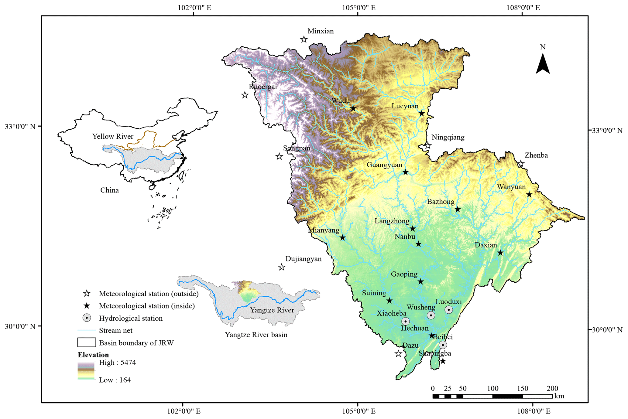
Figure 1Sketch map of the Jialing River basin (JRB) with meteorological stations.
2.2 Data sources
The data required for SWAT modeling and validation consisted of geographic-information, meteorological, and hydrological datasets.
2.2.1 Geographic-information dataset
The geographic dataset included the DEM, land use and land cover data (LULC), and soil properties. SRTM (Shuttle Radar Topography Mission) 90 m resolution data were the DEM used in this study and were provided by the Geospatial Data Cloud (http://www.gscloud.cn/, last access: 7 June 2020). LULC data were obtained by manual visual interpretation based on 2010 Landsat TM/ETM (Thematic Mapper/Enhanced Thematic Mapper) remote sensing images, which were preprocessed by Beijing Digital View Technology Co., Ltd, with a spatial resolution of 30 m. The data included six primary classifications – cultivated land, woodland, grassland, water area, construction land, and unused land – as well as 25 secondary classifications. After checking the quality of data products by combining field survey and random sampling dynamic map spots for repeated interpretation analysis, it is proved that the cultivated land's classification accuracy was 85 %, and other data classification accuracies reached 75 %. The soil data included a soil type distribution map and soil attribute database. The soil type distribution map is a product of the second national land survey provided by the Nanjing Institute of Soil Research, Chinese Academy of Sciences. It depicted a spatial resolution of 1 km and used the FAO-90 (Food and Agriculture Organization) soil classification system. The Harmonized World Soil Database v1.2, which was provided by the Food and Agriculture Organization (FAO), was the soil attribute database used in this study and can be downloaded from http://www.fao.org/land-water/databases-and-software/hwsd/en/, last access: 7 June 2020. Most soil attribute data can be obtained directly from the HWSD (Harmonized World Soil Database) v1.2, such as soil organic carbon content, soil profile maximum root depth, and soil concrete gradation. Parameters that cannot be directly obtained from the HWSD, e.g., texture class, matrix bulk density, field capacity, wilting point, and saturation hydraulic coefficient, can be calculated from the acquired data using the Soil–Plant–Atmosphere–Water Field & Pond Hydrology model developed by Washington State University. All of the above geographic-information data were processed by ArcMap 10.2 to obtain 250 m spatial resolution data of the JRW, using the Beijing_1954_GK_Zone_18N (Gauss–Krüger) projection coordinate system and GCS_Beijing_1954 geographic coordinate system.
2.2.2 Meteorological and hydrological dataset
Daily observed discharges are documented from 1997 to 2018 at the Beibei hydrological station. The daily meteorological records – including precipitation, temperature, relative humidity, sunshine hours, and wind velocity – were measured by 20 meteorological stations in and around the JRW, which were provided by the China Meteorological Data Service Center (http://data.cma.cn/, last access: 7 June 2020). The solar-radiation data required for establishing the meteorological database were calculated using the sunshine hours (n), and the calculation method consisted of employing the solar-radiation (Rs) index in the FAO-56 Penman–Monteith method.
The first gridded format CHIRPS product was released in February 2015, which has first recorded in 1981 and continues to be updated. The dataset provides daily precipitation data with a spatial resolution of 0.05∘ in a pseudo-global coverage of 50∘ N–50∘ S. The data are available for download at http://chg.geog.ucsb.edu/data/chirps/ (last access: 7 June 2020). The CHIRPS product is composed of various types of precipitation products, including ground measurement, remote sensing, and reanalysis data; e.g., the Climate Hazards Group Precipitation Climatology (CHPclim) is built from monthly precipitation data supplied by the United Nations FAO, Global Historical Climate Network (CHCN), Cold Cloud Duration from NOAA, TRMM 3B42 Version 7 from NASA, etc. Essentially, the above-mentioned data were synthesized into 5 d rainfall records, and then the rain gauge observations from multiple data sources were used to correct the deviation, which was further interpolated to the daily-scale CHIRPS product. More detailed information about CHIRPS products is available in Funk et al. (2015).
CPC-Global, in a gridded format, is the first-generation product of NOAA's ongoing CPC unified precipitation project. This product offers daily precipitation estimates from 1998 to the present, at a spatial resolution of 0.5∘ over land. Daily precipitation data for CPC-Global can be downloaded from http://ftp.cpc.ncep.noaa.gov/precip/CPC_UNI_PRCP/GAUGE_GLB/V1.0/ (last access: 7 June 2020). This dataset integrates all existing CPC information sources and employs the optimal-interpolation objective analysis technique to form a set of cohesive precipitation products with consistent quantity and enhanced quality. The data were collected from > 30 000 monitoring stations belonging to the WMO Global Telecommunication System, the Cooperative Observer Network, and other national meteorological agencies (Xie et al., 2007). For the sake of brevity, the CPC-Global data are referred to as CPC in this article, and the corresponding SWAT model is denoted as the CPC model.
In the SWAT model, all meteorological data were categorized into subbasins according to the “nearest-distance” principle. As such, for the point-formatted gauge observations, a SWAT subbasin will read the precipitation records from the weather station that is closest to its centroid. Similarly, for the grid-formatted estimates, i.e., CHIRPS and CPC, a SWAT subbasin will read the precipitation observations from the grid that is closest to its centroid. Using this method, the grid records of high-resolution CHIRPS products within the same subbasin will be uniformly assigned the grid value closest to the centroid, which will offset the high-resolution advantage of CHIRPS products. In order to incorporate the advantages of the CHIRPS model's spatial resolution and the SWAT model's effectiveness when using the other two products, we selected 400 subbasins so that the number of effective CHIRPS is ∼20 times greater than that of Gauge and CPC. Note that all of the precipitation statistics in this study are based on the subbasin scale, which ensures that the precipitation data were correctly categorized in the SWAT model.
2.3 Statistical-analysis method
The following indices were selected to statistically compare the three precipitation products:
-
CC value. The correlation coefficient (CC) is a numerical measure (ranging from −1 to 1) of the linear statistical relationship between two variables, e.g., simulations and observations, with respect to strength and direction. The closer the absolute value of CC is to 1, the higher the correlation between simulation and observation is. CC is mathematically expressed as follows:
where n is the number of the time series; Qi and Si are measured values and estimated values, respectively; and and are the mean values of the measured and estimated values, respectively. The value may refer to either precipitation (mm) or streamflow discharge (m3 s−1).
-
SD value. Standard deviation (SD) represents the discretization degree of the datasets (mm). The SD of Gauge observations is used to normalize the OPPs' SD and, when denoted as SDn, to compare the dispersion of OPPs relative to Gauge. The SDn values range from 0 to ∞, and the optimal value is 1. The SDn value is mathematically expressed as follows:
where SDOPP and SDGauge are the SDs of OPPs and Gauge, respectively.
-
RSR value. RMSE (root mean square error) observation standard deviation ratio (RSR) is an error index statistic between the OPPs and Gauge datasets. Root mean square error (RMSE) divided by SD values would derive the RSR value. RSR has a range from 0 to ∞ with 0 as the optimal value. The calculation equation is expressed as follows:
-
POD value. Probability of detection (POD) is a ratio that reflects the number of times OPPs correctly detected the frequency of rainfall relative to the total number of rainfall events. POD has a range from 0 to 1 and an optimal value of 1. It is mathematically expressed as follows:
where t is the number of qualified data pairs, H denotes when Gauge and OPPs both detect a rainfall event, and M represents when Gauge detects a rainfall event but the OPPs do not.
-
FAR value. False-alarm rate (FAR) represents the frequency that precipitation is detected using OPPs but not detected using Gauge. FAR has a range from 0 to 1 and an optimal value of 0. The FAR value is mathematically expressed as follows:
where F denotes that the OPPs detected a rainfall event, while Gauge does not.
2.4 Hydrological model
2.4.1 SWAT description
The process-based SWAT model is an all-inclusive, temporally uninterrupted, and semi-distributed simulation that was developed by the Agricultural Research Service of the United States Department of Agriculture (Arnold et al., 1998; Arnold and Fohrer, 2005). The model's smallest simulation unit is the Hydrological Response Unit (HRU). Fields with a specific LULC and soil, which may be scattered throughout a subbasin, are lumped together in one HRU. The model assumes that there is no interaction between HRUs in any one subbasin. According to the water balance cycle, the HRU hydrologic process is first calculated and then summed to obtain the total hydrologic process of the subbasin (Arnold et al., 2012). Water balance, including precipitation, surface runoff, actual evapotranspiration, infiltration, lateral and baseflow, and percolation to shallow and deep aquifers, is mathematically expressed as follows:
where SWt is the soil's water content at the end of period t (mm), SW0 is the soil water content at the beginning of period t (mm), and t is the calculation period length. P is precipitation; Qsurf is surface runoff; ET is actual evapotranspiration; Wseep is the amount of percolation and bypass flow exiting the soil profile bottom; Qlat is lateral flow; and Qgw is baseflow, including return flow from the shallow aquifer (GW_Q) and flow out from the deep aquifer (GW_Q_D), all on day i (mm).
Surface runoff, lateral flow, and baseflow add up to water yield (WYLD). SWAT uses the Soil Conservation Services Curve Number method (SCS-CN) to simulate surface runoff. Surface runoff is mathematically expressed as follows:
where Ia is the initial loss (mm), i.e., precipitation loss before surface runoff; F is the final loss, i.e., precipitation loss after surface runoff is generated; and S is the maximum possible retention in the basin at that time (mm) and is the upper limit of F.
The WYLD from the subbasin forms in the connected channel network and then, through routing water processes, enters the downstream reach segment and repeats the water balance process, eventually converging at the drainage outlet. This is the watershed hydrological process simulated in SWAT that is shown in Fig. 2.
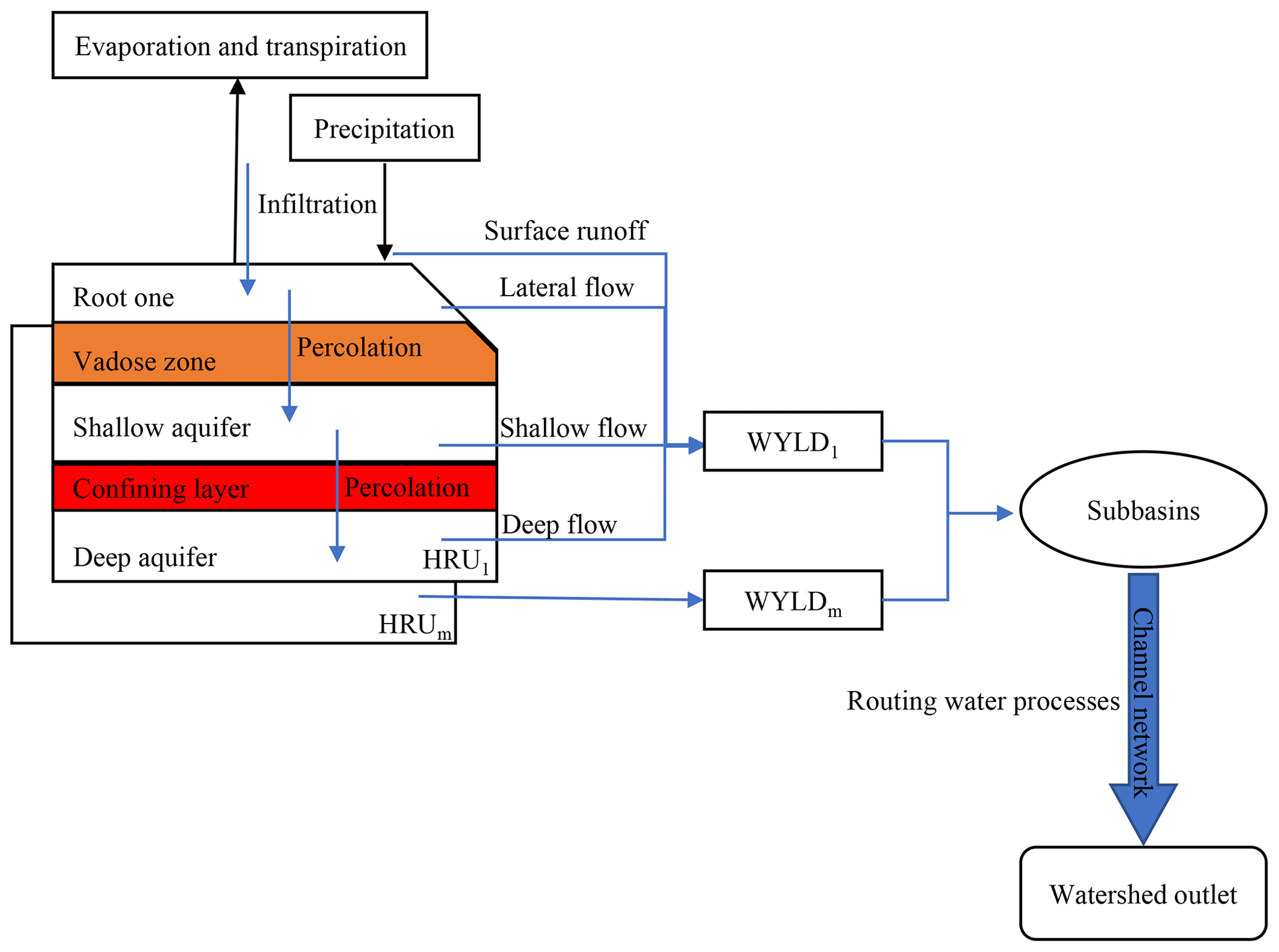
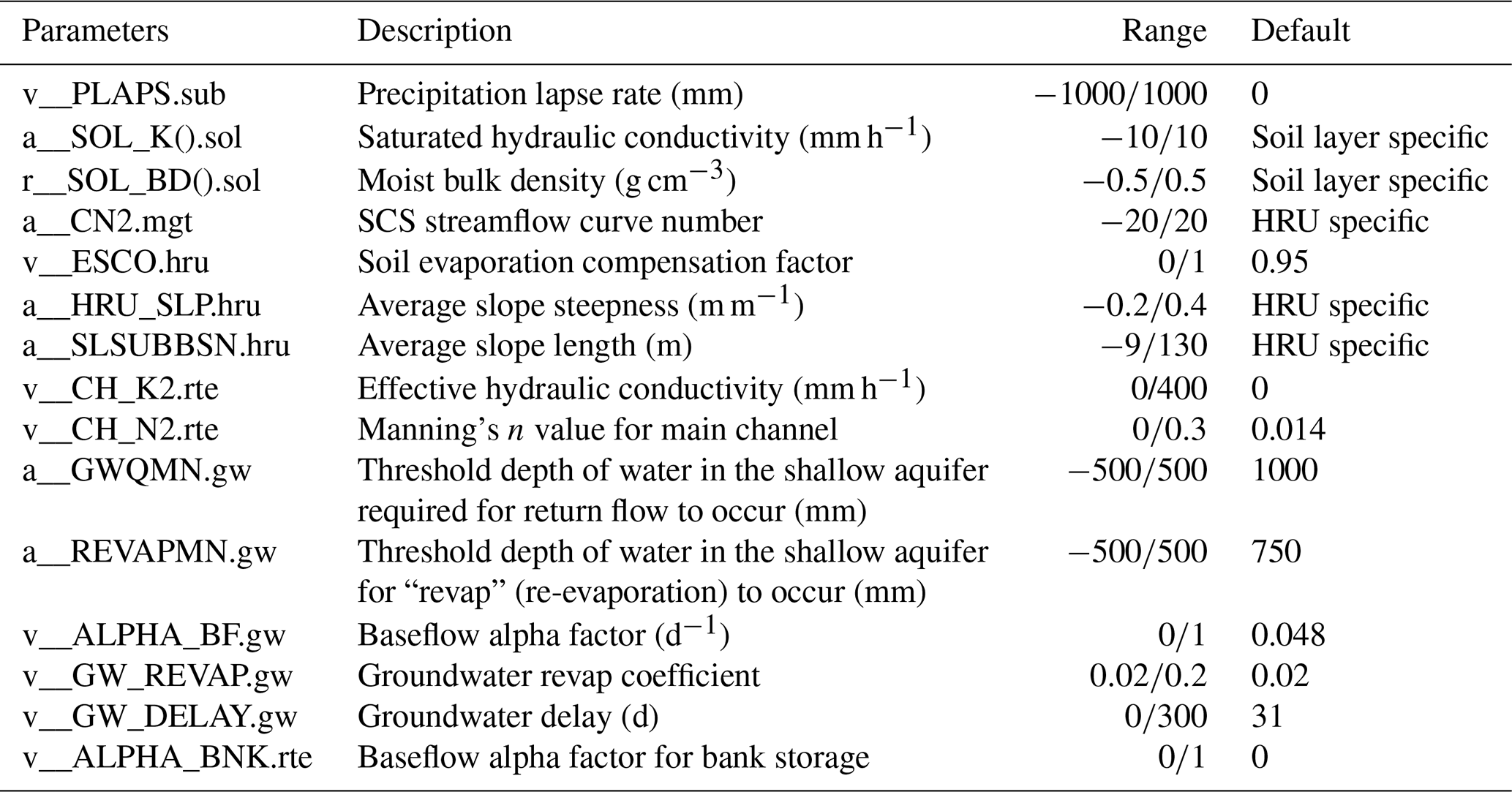
Table 1Hydrological parameters considered for sensitivity analysis (a_, v_, and r_ mean an absolute increase, a replacement, and a relative change to the initial parameter values, respectively).
2.4.2 SWAT calibration and validation
In this study, the period of calibration and validation are set for 1999–2008 and 2009–2018, respectively. The 2 years before both the calibration and validation periods are delineated as the warmup phase for the purpose of initializing model state variables, e.g., soil moisture and groundwater concentration. The model is automatically calibrated using the Sequential Uncertainty Fitting algorithm version 2 (SUFI-2) in the SWAT Calibration and Uncertainty Program (SWAT-CUP). This algorithm has been successfully applied in many related studies (Abbaspour et al., 2017; Shivhare et al., 2018; Tuo et al., 2018). The model parameters and the initial calibration range are shown in Table 1. The parameters were selected based on literature published by Arnold et al. (2012) and Tuo et al. (2016) and the official manual. In order to consider the impact of elevation on precipitation and the fact that precipitation in the OPPs is horizontal, we introduced the precipitation lapse rate (PLAPS) parameter and divided each subbasin into 10 elevation bands. Tuo et al. (2016) demonstrated that this method is able to correct the rainfall error caused by ignoring elevation and effectively improve the model's simulation performance. Furthermore, the models were calibrated following three iterations of 1000 times each. Following each iteration, the SWAT-CUP generated a fresh set of parameter ranges. This new set was used for the next iteration after considering the upper and lower bounds of the physical meaning. The above method was repeated for the three different precipitation datasets. The Nash efficiency coefficient (NSE) was used as the objective function to optimize the model calibration and is mathematically expressed as follows:
Table 2General performance ratings statistics recommended by Moriasi et al. (2007).
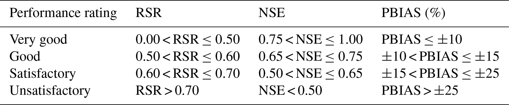
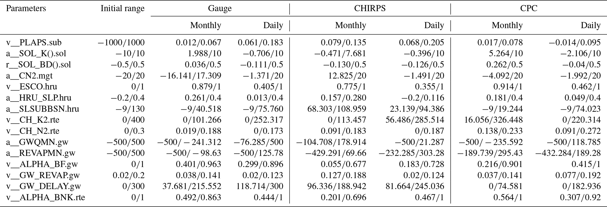
The model performance was classified using RSR, NSE, and percentage bias (PBIAS) values defined by Moriasi et al. (2007), which is shown in Table 2. Parameter ranges of the three models after 3000 iterations are shown in Table 3. CC, NSE, PBIAS, and RSR were used to evaluate the model simulation results.
PBIAS describes the OPPs' systematic bias (%). PBIAS ranges from 0 to +∞ %, and the optimal value is 0 %. The calculation equation is expressed as follows:
The quality of model input data and the parameterization process increase the uncertainty risk associated with the model results, which has been identified in the application of SWAT (Thavhana et al., 2018; Tuo et al., 2018; Zhang et al., 2020). There are two factors, p factor and r factor, which are used for uncertainty analysis in the SUFI-2 algorithm of SWAT CUP; p factor refers to the percentage of the measured data distributed within the 95 % prediction uncertainty (95PPU) band of the model results (%), and the r factor graphically means the average thickness of the 95PPU band divided by the SD of the measured records (Abbaspour, 2017). Theoretically, p factor ranges from 0 to 100 % and takes 100 % as the optimal value, and r factor ranges from 0 to ∞ and takes 0 as the optimal value. It should be noted that the increase in the p factor comes at the expense of the increase in the r factor. It was stated in the study of Roth and Lemann (2016) that combined values of p factor > 70 % and r factor < 1.5 are preferably the uncertainty range, which is also referred to in this paper.
3.1 Evaluation of the OPPs on a temporal scale
3.1.1 Monthly scale
A comparison of the monthly precipitation time series (Gauge, CHIRPS, and CPC) across the watershed is shown in Fig. 3. Note that the time series in Fig. 3 represents the average value of the whole watershed and was calculated as follows: the original point or grid-formatted rainfall records were first categorized into every SWAT model subbasin, according to the nearest-distance principle, and then spatially synthesized into one time series by subbasin area using the weighted-average method. Figure 3 shows that the rainfall values in the rainy season (especially in July) captured by Gauge are higher than those of CHIRPS and CPC. Moreover, the CC values between CHIRPS and Gauge records, as well as CPC and Gauge records, are 0.97 and 0.98 (p < 0.01, i.e., extremely significant positive correlation), respectively. The high CC values demonstrate the highly correlated linear relationship between the two OPPs and Gauge records on a monthly scale, indicating that both CHIRPS and CPC products are equally as effective at describing the monthly precipitation variation within the JRW as the Gauge records.
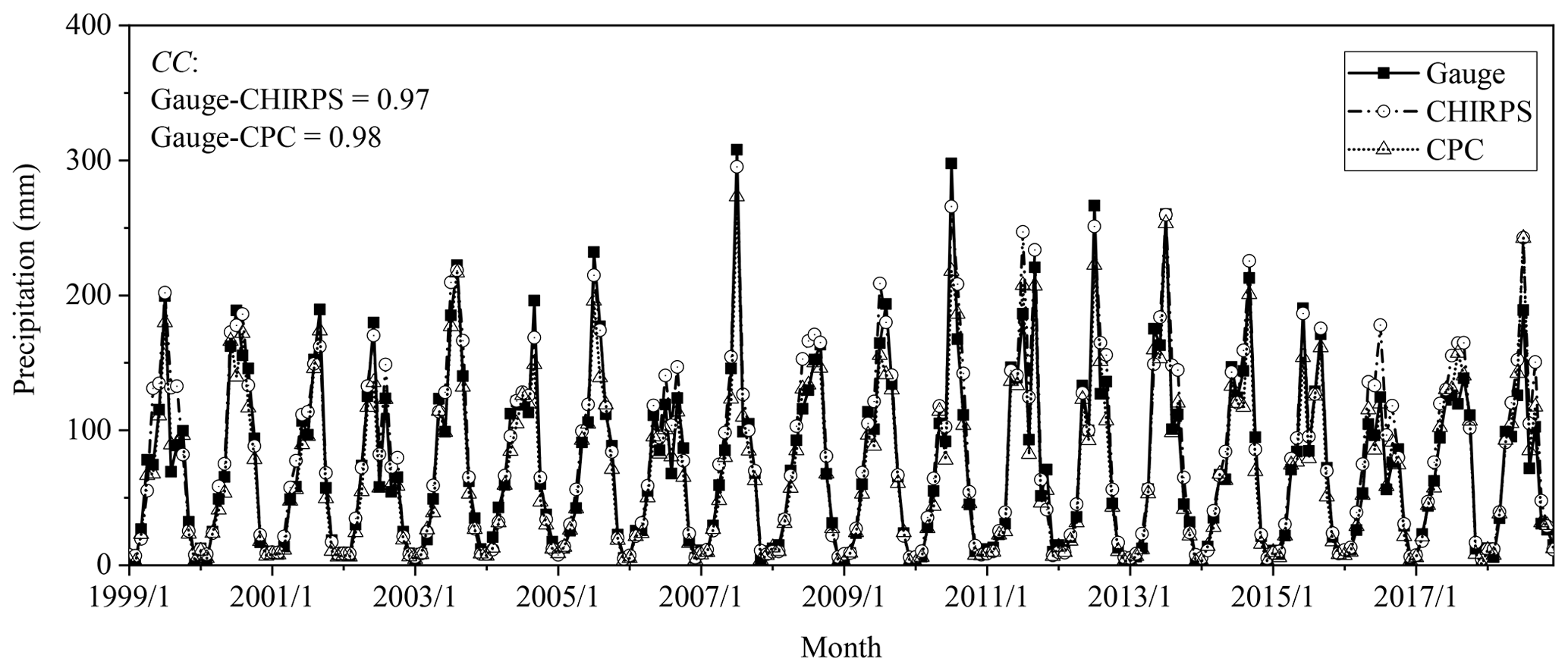
Figure 3Time series of three different precipitation records at a monthly scale in the JRW (the CC values of 0.97 and 0.98 indicate an extremely significant positive correlation; p < 0.01, where p stands for the probability of being rejected when there was a significant difference). Please note that the date in this figure is given as year/month.
The box diagrams of the three precipitation records are shown in Fig. 4. Note that July is the largest contributor to the yearly precipitation, as well as the annual-flood-peak calculation. According to the July results, when compared with Gauge records, the CHIRPS product has a large median, small maximum, and large minimum, while the three CPC values are all smaller than the Gauge values. These characteristics will potentially lead to different hydrological modeling in flood peak simulation. The SDn values for Gauge-CHIRPS and Gauge-CPC are 1.06 and 0.94, respectively. The RSR values for Gauge-CHIRPS and Gauge-CPC are 0.27 and 0.22, respectively. These statistics indicate that both CHIRPS and CPC estimates are able to provide equally effective precipitation values compared with that of the Gauge records. Nevertheless, PBIAS values of Gauge-CHIRPS and Gauge-CPC were 9.58 % and −6.70 %, respectively, indicating the overestimation of CHIRPS products and underestimation of CPC products compared with that of the Gauge records. Specifically, overestimation of the CHIRPS products mainly occurs between April and September, which is the JRW rainy season, while during the dry season, i.e., October–March, the CHIRPS estimates are closely consistent with the Gauge records. In contrast, the CPC estimates parallel the Gauge records for the rainy season, yet rainfall is underestimated during the dry season.
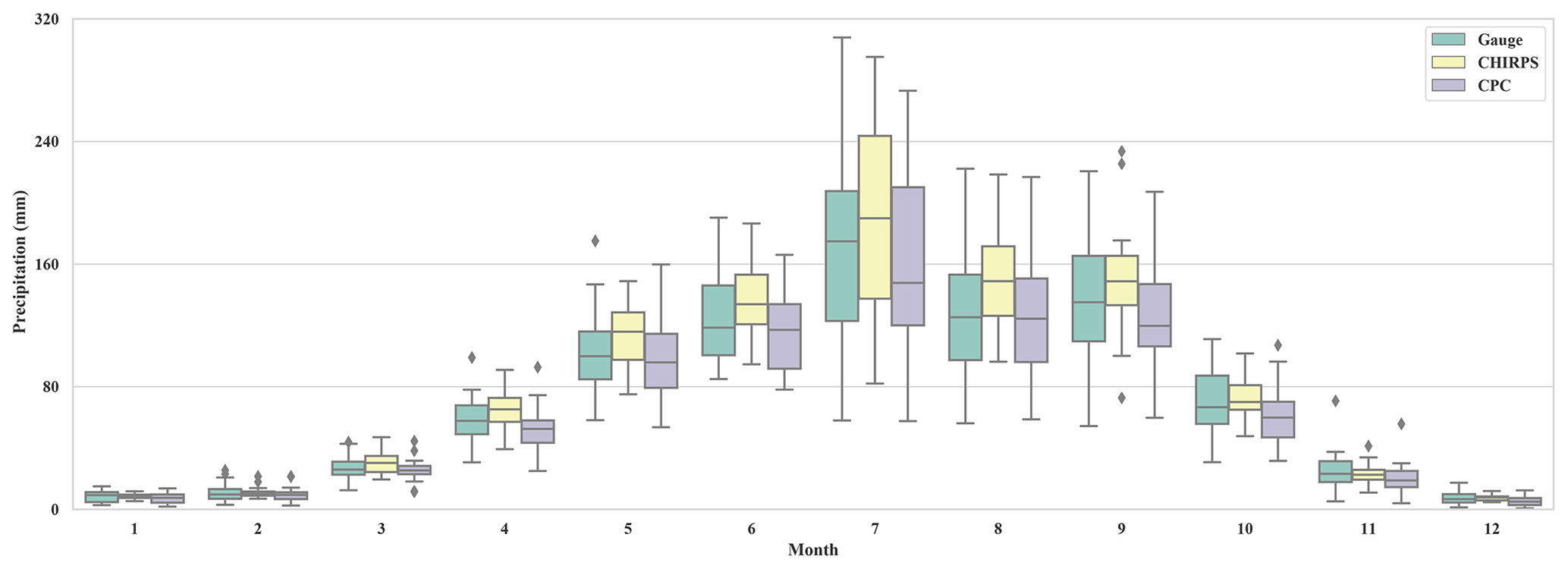
Figure 4Box diagrams of three different precipitation records at a monthly scale in the JRW.
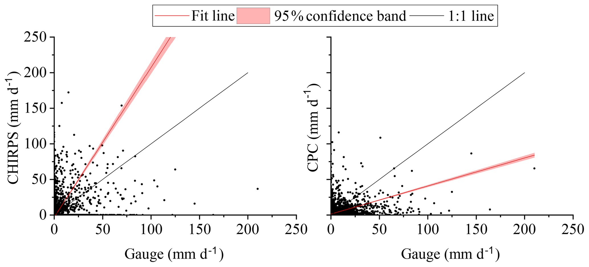
Figure 5Scatterplot of the OPP records compared with Gauge records at a daily scale: (a) comparison of CHIRPS and Gauge and (b) comparisons of CPC and Gauge.
3.1.2 Daily scale
Intensity and frequency are the most critical parameters for characterizing rainfall features on a daily scale (Azarnivand et al., 2019; Wen et al., 2019). The scatterplots in Fig. 5 depict a precipitation intensity comparison between the OPPs and Gauge records, at a daily scale, at Beibei hydrological station (no. 411). Based on Fig. 5, the angle between the CHIRPS model's 95 % line estimates and the horizontal axis is > 45∘ (the 1:1 line), indicating that CHIRPS overestimates precipitation relative to the Gauge records. CPC estimates demonstrate the exact opposite. More specifically, the scatter distribution indicates that compared to the Gauge records, the CHIRPS estimates tend to overestimate precipitation for light rains and underestimate it for heavy rains. Meanwhile, the CPC products underestimate both light and heavy rains. Statistically, the CC, SDn, and RSR values between CHIRPS and the Gauge records are 0.53, 1.14, and 1.04, respectively, and 0.64, 0.87, and 0.80, respectively, between the CPC and Gauge products. At the daily scale, the OPPs and Gauge products showed an evident decrease in consistency when compared with the monthly scale. The above indicators demonstrate the deceased consistency of the OPPs' estimates and Gauge observations, while CPC shows superior performance relative to CHIRPS.
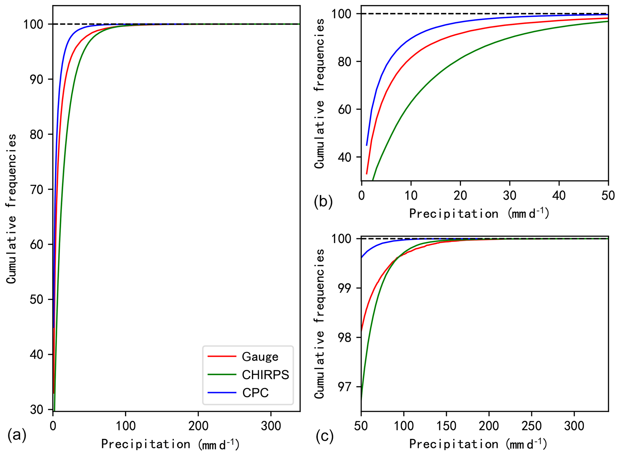
Figure 6Cumulative frequencies of daily precipitation intensity for the three precipitation products (Gauge, CHIRPS, and CPC) in the JRW: (a) distribution of all precipitation values, (b) distribution of precipitation values that are < 100 mm, and (c) distribution of precipitation values that are ≥100 mm.
The three precipitation products' cumulative daily precipitation intensity frequencies are shown in Fig. 6. Note that on the right side of the figure, the 50 mm d−1 demarcation divides the horizontal axis into two sections of rainfall intensity, in order to depict the three products' frequency trends more clearly. Overall, the three products display a high probability of occurrence for precipitation intensity of 0.1–25 mm d−1–87 %, 94 %, and 98 % for CHIRPS, Gauge, and CPC, respectively. However, the probability for precipitation intensity > 100 mm d−1 is 99.70 %, 99.73 % and 99.99 %, respectively, indicating the potential upper-limit extreme-rainfall-event value within this area. The CPC product fails to detect extreme rainstorm events.
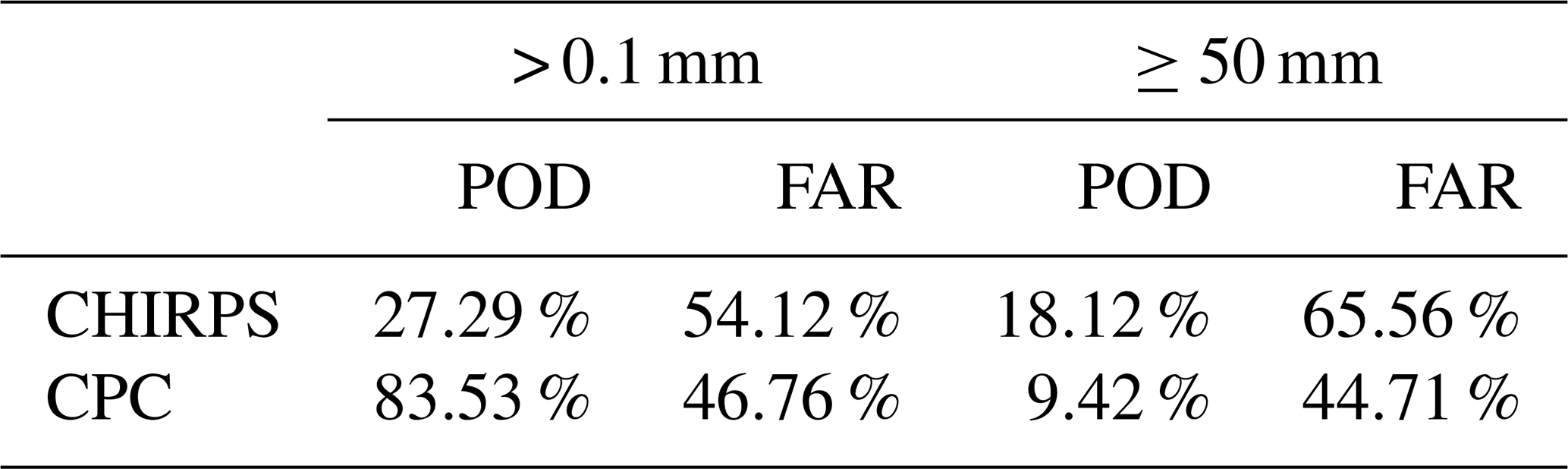
Table 4 is the recognition capability evaluation of the two OPPs for rainfall intensity between 0.1 and 50 mm and > 50 mm events. The CPC and CHIRPS POD values for rainfall intensity between 0.1 and 50 mm are 83.53 % and 27.29 %, respectively, demonstrating that the CPC product has a strong ability to capture the onset of rainfall. Nevertheless, the CPC POD value for rainfall intensities ≥50 mm decreases to 9.42 %, indicating its poor ability to capture rainstorms, while that of the CHIRPS product is relatively higher, with a POD value of 18.12 %. Moreover, the FAR fractions for both OPPs are between 44 % and 66 %, demonstrating its lower ability to detect rainstorm values.
3.2 Evaluation of OPPs on a spatial scale
Spatial variations of the three products' long-term mean annual precipitation, for all of the partitioned subbasins, are shown in Fig. 7. The three products' precipitation values exhibit an obvious upward trend from the JRW's upstream-to-downstream region. The precipitation's shifting pattern in space highly correlates with the topography variation (shown in Fig. 1), indicating that meteorological and hydrologic variables throughout the region are potentially influenced by and respond to catchment landscape modification. It should be noted that in Fig. 7a, all the subbasins are divided into several regions, each of which has the same rainfall value, while abrupt rainfall value changes occurred between adjacent regions. In Fig. 7c, the transition between adjacent subbasins is smoother than that observed with Gauge. In Fig. 7b, the CHIRPS product shows the smoothest precipitation transition between the adjacent subbasins, illustrating the advantages of the high-resolution CHIRPS product. In this study, precipitation records from 20 rain gauge stations, 411 CHIRPS grids, and 76 CPC grids were categorized into the SWAT subbasins (as mentioned in Sect. 2.3), leading to differences in the continuity or smoothness of rainfall spatial distribution among the three products. Compared with the Gauge observations, the overall precipitation values estimated by CHIRPS are relatively higher, while those of CPC are relatively lower.

Figure 7Spatial variation of annual precipitation at a subbasin scale for (a) Gauge, (b) CHIRPS, and (c) CPC.
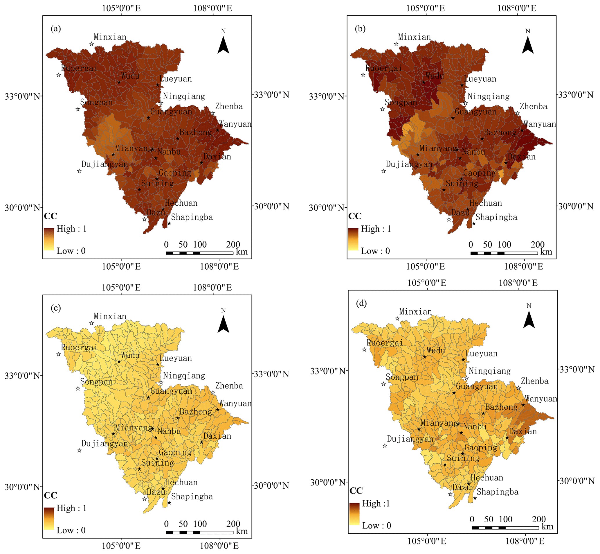
Figure 8Spatial variation of CC values of the precipitation between (a) Gauge and CHIRPS and (b) Gauge and CPC at a monthly scale and (c) Gauge and CHIRPS and (d) Gauge and CPC at a daily scale.
The CC, SDn, and RSR values of precipitation spatial distribution between CHIRPS and Gauge are 0.89, 0.96, and 0.55, respectively, and 0.82, 0.87, and 0.62 between CPC and Gauge, respectively. These statistics indicate that both CHIRPS and CPC estimates can describe the spatial distribution of precipitation in the JRW, among which CHIRPS depicts better performance. The correlation coefficients between Gauge and OPPs at monthly or daily scales for every subbasin are illustrated in Fig. 8. Overall, the monthly-scale CC values (with a range of 0.7–1) are comparably larger than that of the daily-scale values (with a range of 0.5–0.7). Spatially, the higher CC values between Gauge and CPC at the monthly scale are mainly distributed in areas with comparably low or high rainfall amounts, such as Wudu and Wangyuan. Yet, the CC value was less relevant in areas with moderate rainfall (e.g., Suining) relative to that of Gauge and CHIRPS. However, at the daily scale, the correlation of Gauge and CPC is higher than that of Gauge and CHIRPS, except for a few individual subbasins located in the eastern and southern area.
3.3 Hydrological performance of different precipitation products in the SWAT model
3.3.1 Spatiotemporal performance at a monthly scale
OPPs ignore terrain differences when forcing the model, which may increase potentially systematic errors in hydrologic modeling (Tuo et al., 2016). Thus, in this work, elevation bands (see Sect. 2.4.1) were used to normalize precipitation at different elevations. The monthly observed runoff and simulated runoff subjected to this procedure and used for the SWAT model during the calibration and validation periods are presented in Fig. 9. The results show that the three precipitation inputs successfully stimulated the model to reproduce the discharge records at the Beibei station; the rising and falling simulated flood event processes are in good agreement with that of the observed ones. Based on the model performance classification scheme designed by Moriasi et al. (2007), Gauge and CHIRPS achieved very good performance for both the calibration and validation periods, although the Gauge model attained the highest NSE (0.92 for calibration and 0.87 for validation) values and lowest RSR (0.28 and 0.36) values, while CPC only reached the level of good due to higher PBIAS values (10.8 %) (Fig. 9). Further, among all the three models, the model with Gauge inputs performed best in uncertainty analyses (p factor =98 %, r factor = 0.86 for calibration and p factor =92 %, r factor =0.78 for validation), which is followed by the model using CHIRPS as input (p factor =84 %, r factor =0.88 and p factor =83 %, r factor =0.80). Using CPC datasets as precipitation inputs resulted in the highest degree of uncertainty level (p factor =57 %, r factor =0.57 and p factor =57 %, r factor =0.53), which fails to reach a preferable level. The underestimation of the peak flows during flood seasons (June to August) would be the main reason of the slightly worse performance of the two OPPs inputs. The Gauge model demonstrates the best performance, which may reflect its strong ability to ascertain the peak rainfall during the flood seasons (Fig. 4). Note that in Fig. 4, the CHIRPS medians are larger than those of Gauge, while the maxima are smaller, and the minima are larger during the flood seasons. These features facilitated the best performance for describing the baseflow and medium floods, like those in years 2003 and 2014. As a result, the CHIRPS model achieved the best simulation baseflow, although it overestimated the precipitation with light rain intensity and obviously overestimated the streamflow with discharge < 6000 m3 s−1, which also led to its final performance deviation. CPC showed significant overestimation in 2017 and 2018 during the validation period. Although it approximated the CHIRPS model's estimated results, it clearly deviated from its previous tendency to underestimate precipitation during these 2 years.
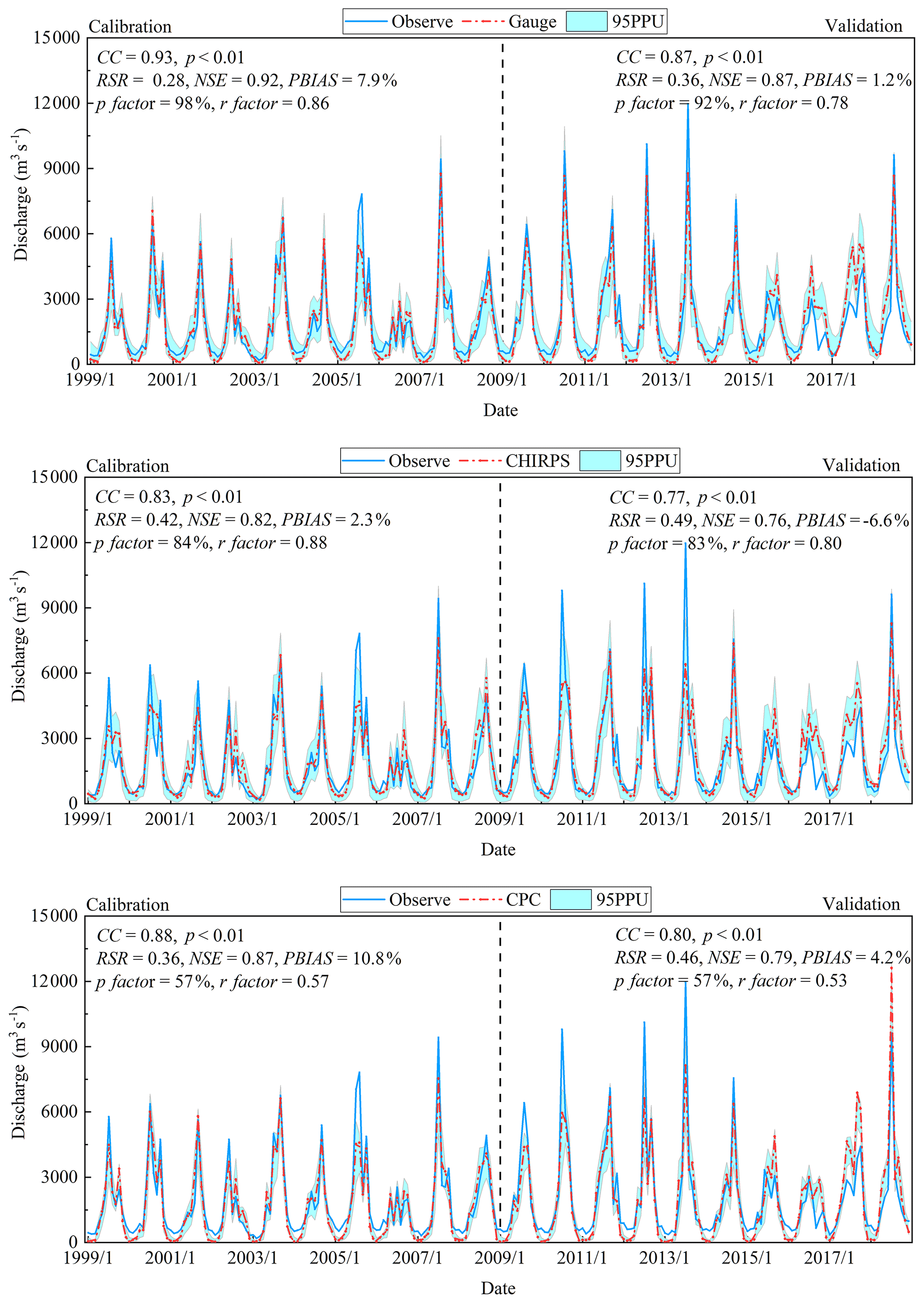
Figure 9Observed and simulated discharges at the outlet of the JRW at a monthly scale using precipitation inputs of Gauge, CHIRPS, and CPC, respectively. Please note that the date in this figure is given as year/month.
In terms of simulated WYLD spatial variation at the subbasin scale (as shown in Fig. 10), the consistency of the Gauge and CHIRPS models is slightly better than that of the CPC model, potentially demonstrating the advantage of the CHIRPS model's high resolution in simulating precipitation. Furthermore, the WYLD distribution pattern is highly consistent with the corresponding precipitation distribution (Fig. 7). The spatial correlation between the WYLD and precipitation for rainfall for the Gauge, CHIRPS, and CPC products reached 0.85, 0.84, and 0.91, respectively. Compared to the Gauge simulation, CHIRPS overestimated and CPC underestimated the WYLD. The Gauge–CHIRPS and Gauge–CPC PBIAS values are 5.85 % and −5.38 %, respectively.
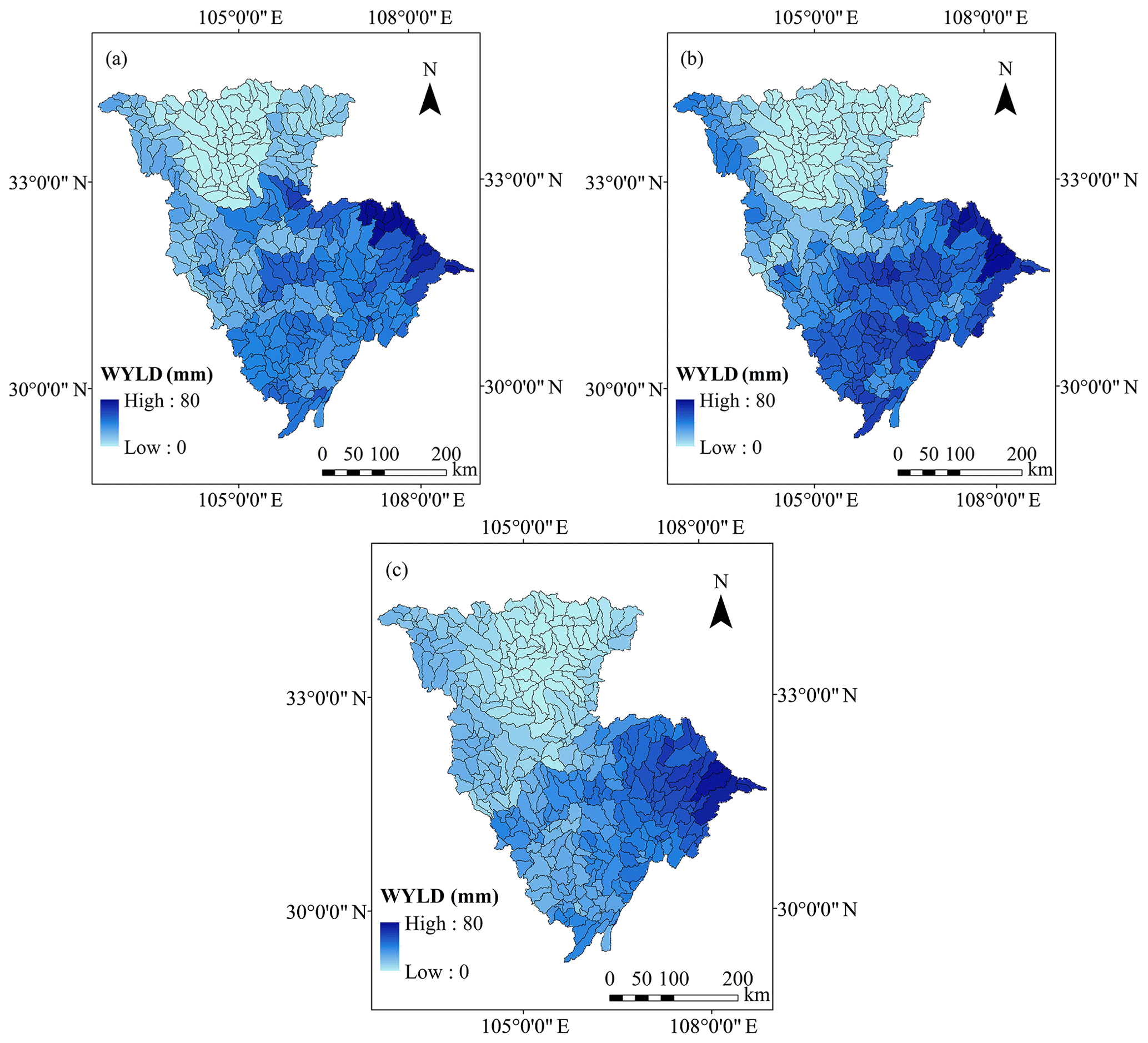
Figure 10Spatial variation of water yield at a monthly scale for all subbasins calculated with precipitation inputs of (a) Gauge, (b) CHIRPS, and (c) CPC.
3.3.2 Spatiotemporal performance at a daily scale
As shown in Fig. 11, the three precipitation inputs also successfully forced the model to replicate the discharge records at the Beibei station at a daily scale, with performance evaluations of good, satisfactory, and satisfactory for Gauge, CHIRPS, and CPC models, respectively. Different from the monthly scale, the CHIRPS-driven daily-scale model showed lowest uncertainty level among the three precipitation datasets. The p factor values of Gauge, CHIRPS, and CPC were 93 %, 95 %, and 77 % for calibration and 84 %, 91 %, and 73 % for validation, respectively, and r factor values were 1.16, 1.25, and 0.98 for calibration and 1.08, 1.27, and 0.93 for validation, respectively. Overall, the uncertainties of daily-scale models with all three precipitation datasets as inputs were significantly lower than those of the monthly scale and the CPC-driven monthly-model success to reach a preferable level. The performances in describing the peak flows were not good for all three products, among which, the Gauge model performs best. The peak flows are usually caused by extreme precipitation events, like rainfall events with an intensity > 80 mm d−1. As shown in Figs. 5 and 6, both CHIRPS and CPC underestimate heavy rainfall intensities compared with the Gauge observations. Conversely, the CHIRPS model performs best in simulating the baseflow, since CHIRPS tends to capture higher values of light rainfalls Gauge and CPC.

Figure 11Observed and simulated discharges at the outlet of the JRW at a daily scale using precipitation inputs of Gauge, CHIRPS, and CPC, respectively. Please note that the date in this figure is given as year/month/day.
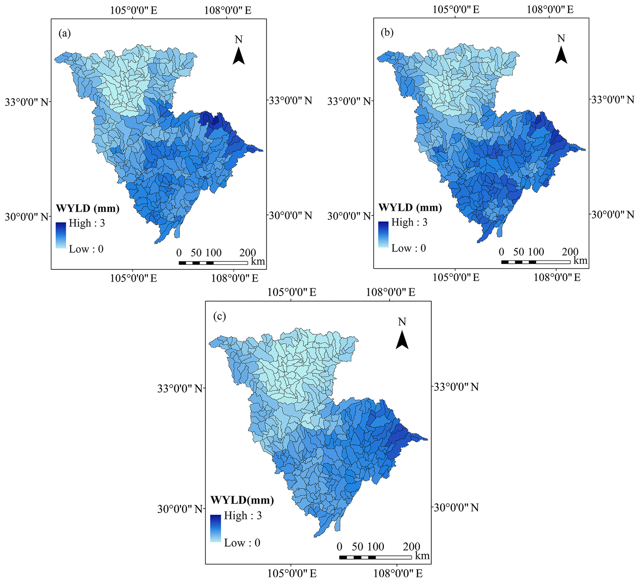
Figure 12Spatial variation of water yield at a daily scale for all subbasins calculated with precipitation inputs of (a) Gauge, (b) CHIRPS, and (c) CPC.
The WYLD spatial variation for all subbasins at the daily scale are shown in Fig. 12. The spatial variation of the daily and monthly scale of the three precipitation datasets is basically the same. The CC values between the daily and monthly WYLD spatial variation for Gauge, CHIRPS, and CPC at the daily scale are 0.98, 0.99, and 0.97, respectively. Similar to the results from the monthly scale, the WYLD spatial pattern is highly correlated with that of precipitation. The CC values between the WYLD and precipitation for Gauge, CHIRPS, and CPC at the daily scale are 0.83, 0.84, and 0.92, respectively, which are even higher than those of the monthly scale. The CC, SDn, and RSR values between CHIRPS and Gauge are 0.92, 1.06, and 0.46, respectively, and 0.81, 0.94, and 0.66 between CPC and Gauge, respectively.
4.1 Comparison of precipitation products in terms of rainfall events with different magnitudes
In the aforementioned results, compared to the Gauge product, CHIRPS tends to overestimate the intensity and frequency of light rain but underestimate heavy rain, which is consistent with the results reported by Gao et al. (2018). However, CPC tends to underestimate the intensity and overestimate the frequency of rainfall for light and heavy rain, although light rain is more underestimated. These results are consistent with those reported by Ajaaj et al. (2019). The differences in the capture of different magnitude rainfall intensities may potentially influence the hydrologic process and forecasting. From Eq. (8), the basin's WYLD is directly proportional to the amount of precipitation. In other words, heavy rainfall tends to produce large amounts of streamflow. J. Duan et al. (2019) conducted a slope experiment and found that there was a significant difference in the runoff coefficients between extreme rainfall events and normal rainfall events; the former produced much more runoff and sediment than the latter. Solano-Rivera et al. (2019) experimented in the San Lorencito headwater catchment and found that the rainfall–runoff dynamics before extreme events were mainly related to antecedent conditions. After extreme flood events, antecedent conditions had no effect on rainfall–runoff processes, and rainfall significantly affected the streamflow discharge. Moreover, the evaluation index NSE performance is mainly determined by the peak streamflow. Thus, it is critical to identify the magnitudes of different rainfall events at both a temporal and spatial scale. As a consequence, we derived the temporal and spatial distributions of the rainfall events with different magnitudes. The spatial scale dimension was implemented by identifying the serial numbers of all subbasins (Fig. 13), and the temporal dimension was fulfilled by detecting rainfall events of different magnitudes throughout the study period (Fig. 14).

Figure 13Spatial distribution of subbasins in SWAT named by numbers.
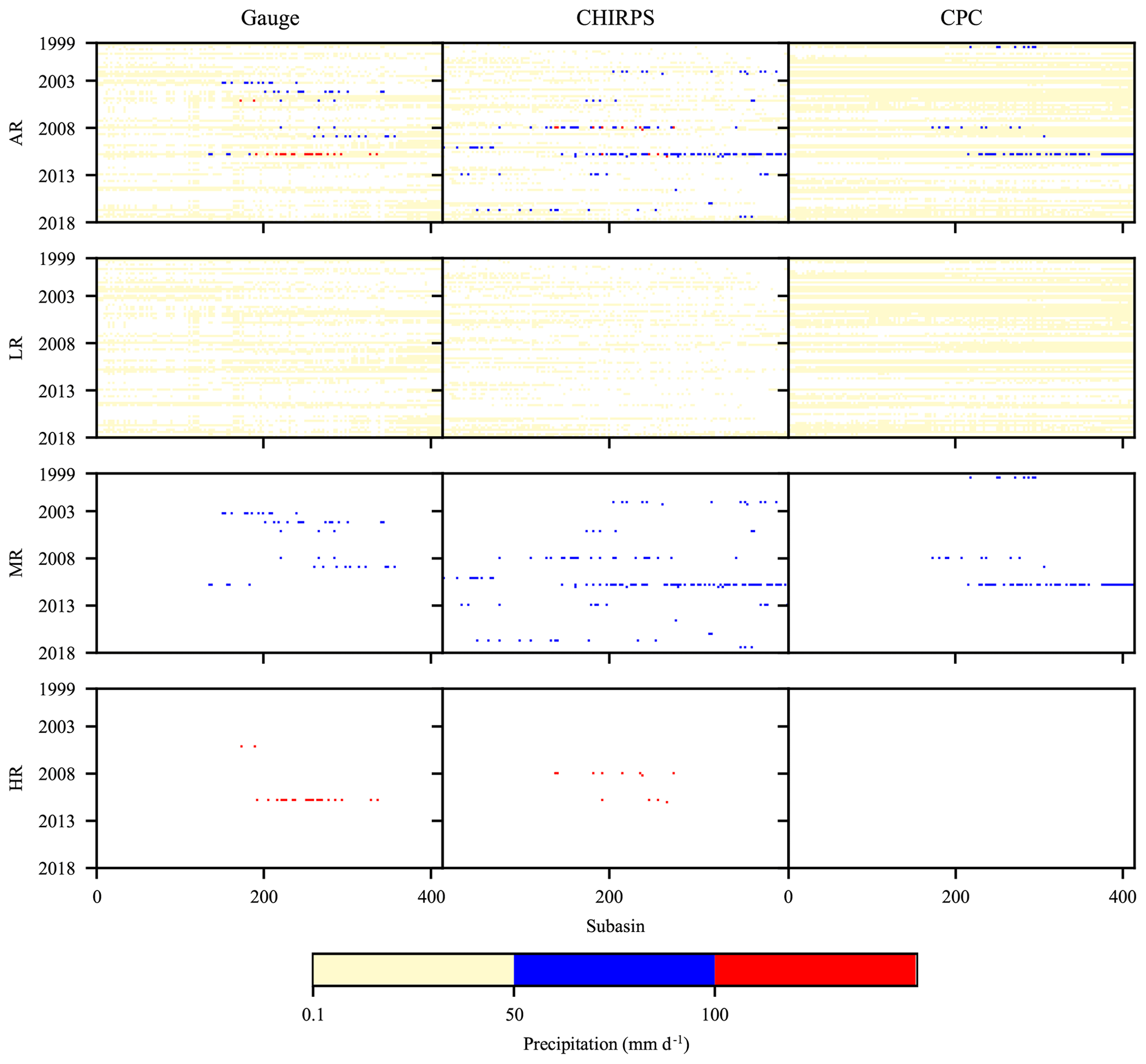
Figure 14Full records of flood events that occurred throughout the study period and all subbasins detected by three precipitation products, where the AR, LR, MR, and HR stand for precipitation of all rainfall intensities, an intensity between 0.1 and 50 mm d−1, an intensity between 50 and 100 mm d−1, and an intensity more than 100 mm d−1, respectively.
Overall, Fig. 14 shows that CPC tends to capture more light rainfall events with precipitation intensities between 0.1 and 50 mm d−1 (LR events), CHIRPS identified more medium rainfall events with precipitation intensities between 50 and 100 mm d−1 (MR events), and both Gauge and CHIRPS detected more heavy rainfall events with precipitation intensities larger than 100 mm d−1 (HR events). Accordingly, the total annual precipitation amounts of the three products are ranked as CHIRPS (956.4 mm) > Gauge (872.8 mm) > CPC (814.3 mm). Even with the advantage of detecting MR and HR events, the ability of CHIRPS to simulate flood events is inferior to that of Gauge. Potential reasons may be that (1) the HR events detected by CHIRPS are more scattered at a temporal scale, which disperses the flood peak value, and (2) the high frequency of the MR detected by CHIRPS resulted in parameter sets in the SWAT model that tended to derive a lower runoff coefficient, in order to avoid a large systematic bias in terms of PBIAS.
The CPC estimates, 60 % of which are detected as LR, tend to be incapable of driving the SWAT model to capture small streamflow discharge, especially the ones equivalent to baseflow. Consequently, the CPC model CC values are relatively low. A potential reason for this phenomenon may be that the rainfall during LR events tends to be easily lost in the initial-loss and post-loss processes, resulting in very limited or even no WYLD. Furthermore, CHIRPS has a high probability of an MR event false alarm, which is consistent with the results reported by Zambrano-Bigiarini et al. (2017). Thus, a significant number of erroneous peaks exist in CHIRPS, just like the temporal variation at a daily scale, which has a very low correlation with Gauge. Erroneous precipitation peaks tend to produce erroneous streamflow peaks. Although SWAT can repair the peak position deviation to some extent, the CC is inevitably reduced.
4.2 Effect of OPPs difference on hydrological-process simulation
In general, simulated and observed streamflow hydrographs, using OPPs and Gauge inputs, can successfully match at both monthly and daily scales. However, consistency between simulated and observed streamflow does not guarantee identical hydrologic processes. For example, the SWAT model calibrated parameters are not the same for all precipitation inputs, meaning that the hydrologic mechanics during SWAT modeling are also different. As such, it is critical that researchers and decision makers adequately understand the benefits and limitations of different precipitation products in modeling the hydrologic processes.
According to the SWAT model's water balance equation (Eq. 7), the WYLD equals the sum of Qsurf, Qlat, and Qg, where Qgw can be divided into flow out from a shallow aquifer (GW_Q) and flow out from a deep aquifer (GW_Q_D). If the soil water content W and percolation and bypass flow into the deep aquifer wseep remains unchanged over a long time period, then the equation is modified to P=Qsurf + ET + Qlat + Qgw. Thus, we calculated the water balance component portions, Qsurf, Qlat, Qgw, and ET, for all the JRW subbasins. With differing parameterizations, different precipitation inputs tend to derive completely different hydrological component amounts at different timescales (Fig. 15 and Table 5). At a monthly scale, all three models, with Gauge, CHIRPS, and CPC as inputs, have similar ET portions, which account for above 54 %. The major components of the Gauge model are surface runoff (SURQ) and lateral flow (LATQ), accounting for 25.92 % and 16.72 %, respectively, the major component of the CHIRPS model is SURQ, which accounts for 34.80 %, and the primary component of CPC model is LATQ, which accounts for 33.62 %. However, at a daily scale, SURQ of the Gauge model increased largely, reaching a proportion of 32.61 %, while LATQ decreased to 10.92 %; LATQ of the CPC model decreased and SURQ, and ET increased, accounting for 14.41 %, 15.60 %, and 58.73 %, respectively; water balance components proportions of the CHIRPS model slightly changed.
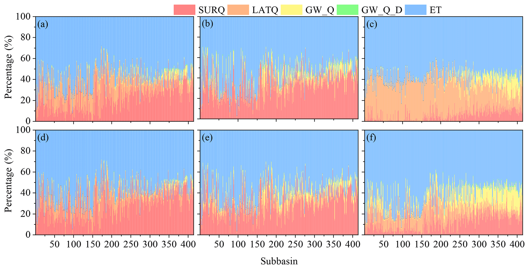
Figure 15Water balance components for all subbasins derived from SWAT models using precipitation inputs of (a) Gauge, (b) CHIRPS, and (c) CPC at a monthly scale and (d) Gauge, (e) CHIRPS, and (f) CPC at a daily scale, where SURQ represents surface runoff Qsurf, LATQ represents lateral flow Qlat, GW_Q is the baseflow from the shallow aquifer, GW_Q_D is the baseflow from the deep aquifer, and the sum of GW_Q and GW_Q_D equals Qgw. ET represents actual evapotranspiration.
Table 5Summarization of water balance components of the three models for the whole JRW.
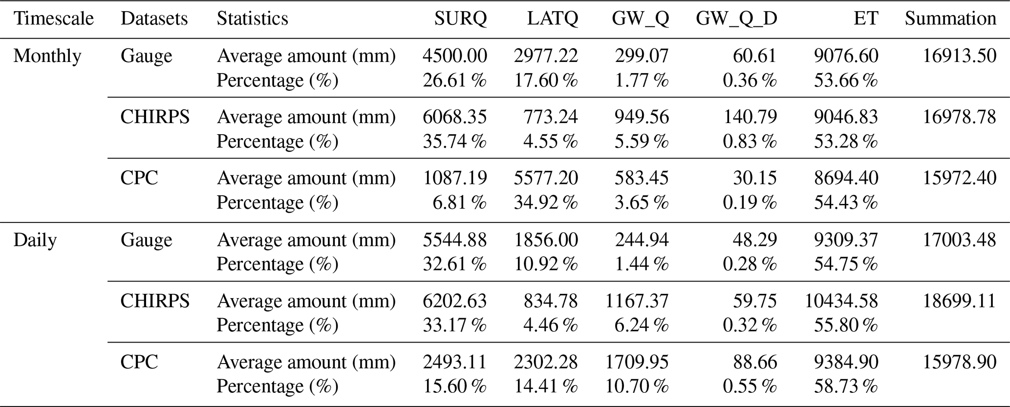
The above water balance component regularities are primarily the result of two causes. First, the differences in the above hydrological component proportions are highly possibly related in parameter adjustment. As shown in Table 3, the SURQ values of Gauge and CPC models were significantly increased due to the decrease of the parameter SOL_K, which stands for saturated hydraulic conductivity. The decrease of the parameter ESCO (soil evaporation compensation factor) in the CPC model led to the increase of the ET ratio, which influenced soil evaporation compensation. The variation of parameter ALPHA_BF, which is a baseflow recession constant, caused the GW_Q components of the three models to vary in the same direction. This result is consistent with that reported by Bai and Liu (2018), who conducted a study at the source regions of the Yellow River and Yangtze River basins in the Tibetan Plateau. They further concluded that the impact of different precipitation inputs on runoff simulation is largely offset by parameter calibration, resulting in significant differences in evaporation and storage estimates.
Second, rainfall characteristics also have a significant impact on hydrological processes in the watershed. A large number of studies show that rainfall intensity is a key player in the watershed's hydrological process (Zhou et al., 2017; Du et al., 2019; Zhang et al., 2019). Studies conducted by Redding and Devito (2010) showed that the occurrence of lateral flow is mainly determined by rainfall intensity. When the rainfall intensity is greater than the surface soil hydraulic conductivity, the rainfall mainly forms surface runoff. When rainfall intensity is between the soil surface and bedrock hydraulic conductivity, the rainfall mainly forms lateral flow. When rainfall intensity is less than the bedrock's hydraulic conductivity, the rainfall will infiltrate into the groundwater. In this study, the precipitation recorded by CHIRPS was mainly distributed between 25 and 100 mm d−1, while that of CPC was mainly distributed between 0.1 and 25 mm d−1. This may be the reason why CHIRPS overestimated the proportion of surface runoff and CPC overestimated the proportion of lateral flow, compared with the Gauge model. Moreover, precipitation in the watershed's upstream area tended to infiltrate into the land surface due to the lower precipitation detection (see Fig. 7), yet when the river flow converged in the watershed's downstream area, the surface flow increased due to the larger detected precipitation values. The results of these findings demonstrated that although the river runoff values simulated by the three models are basically consistent, hydrologic components exhibited distinct behaviors due to the different features in precipitation detection. CHIRPS has a stronger ability to recognize heavy rain and tends to produce more surface runoff, while CPC's strong ability to identify light rain produces more lateral flow. As such, a multi-objective calibration approach would be recommended for flood prediction in future climate. Tuo et al. (2018) use water yield (WYLD) and snow water equivalent (SWE), combining the WYLD and SWE as objectives for parameter calibration and optimization in the SWAT model, and verified the effectiveness of the multi-object procedure.
The sparsity and unevenness of ground-based precipitation observations pose great challenges to the establishment of hydrological models. In this study, Gauge, CHIRPS, and CPC were evaluated by statistically comparing the different precipitation products as well as their performance at driving the hydrological model. Specifically, the potential behaviors of different precipitation datasets in describing precipitation magnitudes and hydrologic processes in terms of water balance components are further discussed. The main conclusions are summarized as follows:
-
The three precipitation datasets exhibited similar temporal records at a monthly scale, and the Gauge measures were more capable of capturing maxima than those of the OPPs. During rainy seasons, the CHIRPS median, maxima, and minima were larger, smaller, and larger, respectively, than those of the Gauge records, while all three CPC statistical values were smaller than those of Gauge. At a daily scale, CHIRPS tends to overestimate light rains and underestimate heavy rains, while all the CPC rainfall intensities were underestimated. Spatially, precipitation in all subbasins increases from the upstream to the downstream region, and CHIRPS derives the most smoothly distributed precipitation pattern.
-
All three precipitation inputs successfully forced the model to replicate the discharge records at the Beibei station at monthly and daily scales, and results at a monthly scale presented slightly better performance than that of a daily scale. However, the differences of precipitation inputs in the statistics at monthly and daily scales correspondingly affected the streamflow hydrograph, e.g., flood peak, base flow, and the rising and falling processes. Overall, the CHIRPS dataset performs better in hydrological evaluation because of its lower uncertainty level and higher spatial accuracy than that of CPC; thus it can be a fairly good option for researchers who are interested in this study area. The three models' spatial WYLD distributions are highly correlated to that of the precipitation records. While there were equivalent performances in simulating streamflow hydrographs, it should be noted that the calibrated parameters in all three models (Gauge, CHIRPS, and CPC models at monthly and daily scales, see Table 3) were quite different. In other words, evaluating only the streamflow simulation accuracy of the precipitation products will conceal the differences between these precipitation products, which is primarily because that hydrological models are able to offset the influences of precipitation inputs on streamflow simulations using parameter calibration and validation.
-
The calibrated parameters are adjusted to alter the hydrologic mechanics in terms of water balance components. Thus, they effectively fill the potential gaps in the WYLD that may be introduced by the varying precipitation amounts and intensities detected by different precipitation products. In particular, according to parameter adjustment, the three products' precipitation detection features resulted in significantly different water balance component portions, i.e., the overestimation of MR by CHIRPS resulted in a larger portion of surface flow, while the underestimation of all rainfall by CPC reduced a larger portion of lateral flow. Multi-objective calibration would be recommended for hydrological modelers in parameter calibration and optimization, especially for large and spatially resolved watersheds. Lastly, the spatial precipitation pattern also significantly impacted the spatial distribution of the water balance components from upstream to downstream.
Although the OPPs have advantages and limitations with respect to the accuracy of precipitation estimates at different spatial and temporal scales, as well as in hydrological modeling and describing hydrologic mechanics, they demonstrate good potential in our case study within the JRW. As such, the OPPs should merge the advantages of satellite, ground observations, and the reanalyzed data. Full consideration of performing the hydrological evaluation from both spatial and temporal scales is also key for the future development of OPPs. Furthermore, CHIRPS is advantaged in extreme-rainfall detection and thus good as flood prediction, while CPC would be more potentially used in extreme drought analysis in future climate analyses and hydrologic modeling.
Sources of the geospatial and climate forcing data used to configure the SWAT model have been described in section 2.2., “Data sources”. The simulations of streamflow data are shown in the figures of the paper and are available through contacting the authors.
HZ conceptualized the work. HZ and JP designed the core structure and collected the data required. JP conducted the data analyses and model simulation and drafted the paper. HZ revised the paper. QX collected data and contributed to key analyses and discussions. YJW, YQW, and OZ contributed to the discussion of the results, and JH assisted in carrying out model configuration and data analyses.
The authors declare that they have no conflict of interest.
This study was supported by the Fundamental Research Funds for the Central Universities (no. 2016ZCQ06), the Joint Fund of State Key Laboratory of Hydroscience and Institute of Internet of Waters Tsinghua–Ningxia Yinchuan (no. sklhse-2019-Iow08), the National Natural Science Foundation of China (nos. 51309006 and 41790434), and the National Major Hydraulic Engineering Construction Funds “Research Program on Key Sediment Problems of the Three Gorges Project” (no. 12610100000018J129-01). We gratefully acknowledge the Beijing Municipal Education Commission for their financial support through the Innovative Transdisciplinary Program “Ecological Restoration Engineering”. We also sincerely thank the anonymous reviewers and editor for their constructive comments and suggestions.
This research has been supported by the Fundamental Research Funds for the Central Universities (grant no. 2016ZCQ06), the Joint Fund of State Key Laboratory of Hydroscience and Institute of Internet of Waters Tsinghua–Ningxia Yinchuan (no. sklhse-2019-Iow08), the National Natural Science Foundation of China (grant nos. 51309006 and 41790434), and the National Major Hydraulic Engineering Construction Funds “Research Program on Key Sediment Problems of the Three Gorges Project” (grant no. 12610100000018J129-01).
This paper was edited by Thomas Kjeldsen and reviewed by two anonymous referees.
Abbaspour, K., Vaghefi, S., and Srinivasan, R.: A Guideline for Successful Calibration and Uncertainty Analysis for Soil and Water Assessment: A Review of Papers from the 2016 International SWAT Conference, Water, 10, 6, https://doi.org/10.3390/w10010006, 2017.
Ajaaj, A. A., Mishra, A. K., and Khan, A. A.: Evaluation of Satellite and Gauge-Based Precipitation Products through Hydrologic Simulation in Tigris River Basin under Data-Scarce Environment, J. Hydrol. Eng., 24, 05018033, https://doi.org/10.1061/(asce)he.1943-5584.0001737, 2019.
Alijanian, M., Rakhshandehroo, G. R., Mishra, A. K., and Dehghani, M.: Evaluation of satellite rainfall climatology using CMORPH, PERSIANN-CDR, PERSIANN, TRMM, MSWEP over Iran, Int. J. Climatol., 37, 4896–4914, https://doi.org/10.1002/joc.5131, 2017.
Arnold, J. G. and Fohrer, N.: SWAT2000 – Current capabilities and research opportunities in applied watershed modelling, Hydrol. Process., 19, 563–572, https://doi.org/10.1002/hyp.5611, 2005.
Arnold, J. G., Srinivasan, R., Muttiah, R. S., and Williams, J. R.: Large area hudrologic modeling and assessment part I: model development1, J. Am. Water. Resour. Assoc., 34, 73–89, https://doi.org/10.1111/j.1752-1688.1998.tb05961.x, 1988.
Arnold, J. G., Moriasi, D. N., Gassman, P. W., Abbaspour, K. C., White, M. J., Srinivasan, R., Santhi, C., Harmel, R. D., van Griensven, A., Liew, M. W. V., and Jha, M. K.: SWAT: Model Use, Calibration, and Validation, T. ASABE., 55, 1491–1508, https://doi.org/10.13031/2013.42256, 2012.
Ayana, E. K., Worqlul, A. W., and Steenhuis, T. S.: Evaluation of stream water quality data generated from MODIS images in modeling total suspended solid emission to a freshwater lake, Sci. Total. Environ., 523, 170–177, https://doi.org/10.1016/j.scitotenv.2015.03.132, 2015.
Azarnivand, A., Camporese, M., Alaghmand, S., and Daly, E.: Simulated response of an intermittent stream to rainfall frequency patterns, Hydrol. Process., 34, 615–632, https://doi.org/10.1002/hyp.13610, 2019.
Bai, P. and Liu, X.: Evaluation of Five Satellite-Based Precipitation Products in Two Gauge-Scarce Basins on the Tibetan Plateau, Remote Sensing, 10, 1316, https://doi.org/10.3390/rs10081316, 2018.
Beck, H. E., van Dijk, A. I. J. M., Levizzani, V., Schellekens, J., Miralles, D. G., Martens, B., and de Roo, A.: MSWEP: 3-hourly 0.25∘ global gridded precipitation (1979–2015) by merging gauge, satellite, and reanalysis data, Hydrol. Earth Syst. Sci., 21, 589–615, https://doi.org/10.5194/hess-21-589-2017, 2017.
Belete, M., Deng, J., Wang, K., Zhou, M., Zhu, E., Shifaw, E., and Bayissa, Y.: Evaluation of satellite rainfall products for modeling water yield over the source region of Blue Nile Basin, Sci. Total. Environ., 708, 134834, https://doi.org/10.1016/j.scitotenv.2019.134834, 2019.
Bohnenstengel, S. I., Schlunzen, K. H., and Beyrich, F.: Representativity of in situ precipitation measurements – A case study for the LITFASS area in North-Eastern Germany, J. Hydrol., 400, 387–395, https://doi.org/10.1016/j.jhydrol.2011.01.052, 2011.
Cecinati, F., Moreno-Ródenas, A. M., Rico-Ramirez, M. A., ten Veldhuis, M. C., and Langeveld, J. G.: Considering Rain Gauge Uncertainty Using Kriging for Uncertain Data, Atmosphere, 9, 446, https://doi.org/10.3390/atmos9110446, 2018.
Cornelissen, T., Diekkruger, B., and Bogena, H. R.: Using High-Resolution Data to Test Parameter Sensitivity of the Distributed Hydrological Model HydroGeoSphere, Water, 8, 202, https://doi.org/10.3390/w8050202, 2016.
Du, J., Niu, J., Gao, Z., Chen, X., Zhang, L., Li, X., and Zhu, Z.: Effects of rainfall intensity and slope on interception and precipitation partitioning by forest litter layer, CATENA, 172, 711–718, https://doi.org/10.1016/j.catena.2018.09.036, 2019.
Duan, J., Liu, Y. J., Yang, J., Tang, C. J., and Shi, Z. H.: Role of groundcover management in controlling soil erosion under extreme rainfall in citrus orchards of southern China, J. Hydrol., 582, 124290, https://doi.org/10.1016/j.jhydrol.2019.124290, 2019.
Duan, Z., Liu, J., Tuo, Y., Chiogna, G., and Disse, M.: Evaluation of eight high spatial resolution gridded precipitation products in Adige Basin (Italy) at multiple temporal and spatial scales, Sci. Total. Environ., 573, 1536–1553, https://doi.org/10.1016/j.scitotenv.2016.08.213, 2016.
Duan, Z., Tuo, Y., Liu, J., Gao, H., Song, X., Zhang, Z., Yang, L., and Mekonnen, D. F.: Hydrological evaluation of open-access precipitation and air temperature datasets using SWAT in a poorly gauged basin in Ethiopia, J. Hydrol., 569, 612–626, https://doi.org/10.1016/j.jhydrol.2018.12.026, 2019.
Ehsan Bhuiyan, M. A., Nikolopoulos, E. I., Anagnostou, E. N., Polcher, J., Albergel, C., Dutra, E., Fink, G., Martínez-de la Torre, A., and Munier, S.: Assessment of precipitation error propagation in multi-model global water resource reanalysis, Hydrol. Earth Syst. Sci., 23, 1973–1994, https://doi.org/10.5194/hess-23-1973-2019, 2019.
Funk, C., Peterson, P., Landsfeld, M., Pedreros, D., Verdin, J., Shukla, S., Husak, S., Rowland, J., Harrison, L., Hoell, A., and Michaelsen, J.: The climate hazards infrared precipitation with stations – a new environmental record for monitoring extremes, Sci. Data., 2, 150066, https://doi.org/10.1038/sdata.2015.66, 2015.
Gabriel, M., Knightes, C., Dennis, R., and Cooter, E.: Potential Impact of Clean Air Act Regulations on Nitrogen Fate and Transport in the Neuse River Basin: a Modeling Investigation Using CMAQ and SWAT, Environ. Model. Assess., 19, 451–465, https://doi.org/10.1007/s10666-014-9410-x, 2014.
Galván, L., Olías, M., Izquierdo, T., Cerón, J. C., and Villarán, R. F.: Rainfall estimation in SWAT: An alternative method to simulate orographic precipitation, J. Hydrol., 509, 257–265, https://doi.org/10.1016/j.jhydrol.2013.11.044, 2014.
Gao, F., Zhang, Y., Ren, X., Yao, Y., Hao, Z., and Cai, W.: Evaluation of CHIRPS and its application for drought monitoring over the Haihe River Basin, China, Nat. Hazards., 92, 155–172, https://doi.org/10.1007/s11069-018-3196-0, 2018.
Gao, Z., Long, D., Tang, G., Zeng, C., Huang, J., and Hong, Y.: Assessing the potential of satellite-based precipitation estimates for flood frequency analysis in ungauged or poorly gauged tributaries of China's Yangtze River basin, J. Hydrol., 550, 478–496, https://doi.org/10.1016/j.jhydrol.2017.05.025, 2017.
Herath, I. K., Ye, X., Wang, J., and Bouraima, A. K.: Spatial and temporal variability of reference evapotranspiration and influenced meteorological factors in the Jialing River Basin, China, Theor. Appl. Climatol., 131, 1417–1428, https://doi.org/10.1007/s00704-017-2062-4, 2017.
Huang, Y., Bárdossy, A., and Zhang, K.: Sensitivity of hydrological models to temporal and spatial resolutions of rainfall data, Hydrol. Earth Syst. Sci., 23, 2647–2663, https://doi.org/10.5194/hess-23-2647-2019, 2019.
Hwang, Y., Clark, M. P., and Rajagopalan, B.: Use of daily precipitation uncertainties in streamflow simulation and forecast, Stoch. Env. Res. Risk. A., 25, 957–972, https://doi.org/10.1007/s00477-011-0460-1, 2011.
Jiang, L. and Bauer-Gottwein, P.: How do GPM IMERG precipitation estimates perform as hydrological model forcing? Evaluation for 300 catchments across Mainland China, J. Hydrol., 572, 486–500, https://doi.org/10.1016/j.jhydrol.2019.03.042, 2019.
Jiang, S., Ren, L., Xu, C., Yong, B., Yuan, F., Liu, Y., Yang, X., and Zeng, X.: Statistical and hydrological evaluation of the latest Integrated Multi-satellite Retrievals for GPM (IMERG) over a midlatitude humid basin in South China, Atmos. Res., 214, 418–429, https://doi.org/10.1016/j.atmosres.2018.08.021, 2018.
Jin, X., He, C., Zhang, L., and Zhang, B.: A Modified Groundwater Module in SWAT for Improved Streamflow Simulation in a Large, Arid Endorheic River Watershed in Northwest China, Chinese. Geogr. Sci., 28, 47-60, https://doi.org/10.1007/s11769-018-0931-0, 2018.
Lai, C., Zhong, R., Wang, Z., Wu, X., Chen, X., Wang, P., and Lian, Y.: Monitoring hydrological drought using long-term satellite-based precipitation data, Sci. Total. Environ., 649, 1198–1208, https://doi.org/10.1016/j.scitotenv.2018.08.245, 2019.
Li, D., Christakos, G., Ding, X., and Wu, J.: Adequacy of TRMM satellite rainfall data in driving the SWAT modeling of Tiao xi catchmen, J. Hydrol., 556, 1139–1152, https://doi.org/10.1016/j.jhydrol.2017.01.006, 2018.
Liu, J. B., Kummerow, C. D., and Elsaesser, G. S.: Identifying and analysing uncertainty structures in the TRMM microwave imager precipitation product over tropical ocean basins, Int. J. Remote. Sens., 38, 23–42, https://doi.org/10.1080/01431161.2016.1259676, 2017.
Lobligeois, F., Andréassian, V., Perrin, C., Tabary, P., and Loumagne, C.: When does higher spatial resolution rainfall information improve streamflow simulation? An evaluation using 3620 flood events, Hydrol. Earth Syst. Sci., 18, 575–594, https://doi.org/10.5194/hess-18-575-2014, 2014.
Long, Y. P., Zhang, Y. N., and Ma, Q. M.: A Merging Framework for Rainfall Estimation at High Spatiotemporal Resolution for Distributed Hydrological Modeling in a Data-Scarce Area, Remote Sensing, 8, 599, https://doi.org/10.3390/rs8070599, 2016.
Lu, Y. J., Jiang, S. H., Ren, L. L., Zhang, L. Q., Wang, M. H., Liu, R. L., and Wei, L.Y.: Spatial and Temporal Variability in Precipitation Concentration over Mainland China, 1961–2017, Water, 11, 881, https://doi.org/10.3390/w11050881, 2019.
Luo, X., Wu, W., He, D., Li, Y., and Ji, X.: Hydrological Simulation Using TRMM and CHIRPS Precipitation Estimates in the Lower Lancang-Mekong River Basin, Chinese. Geogr. Sci., 29, 13–25, https://doi.org/10.1007/s11769-019-1014-6, 2019.
Meng, C. C., Zhang, H. L. Wang, Y. J., Wang, Y. Q., Li, J., and Li, M.: Contribution Analysis of the Spatial-Temporal Changes in Streamflow in a Typical Elevation Transitional Watershed of Southwest China over the Past Six Decades, Forests, 10, 495, https://doi.org/10.3390/f10060495, 2019.
Mileham, L., Taylor, R., Thompson, J., Todd M., and Tindimugaya, C.: Impact of rainfall distribution on the parameterisation of a soil-moisture balance model of groundwater recharge in equatorial Africa, J. Hydrol., 359, 46–58, https://doi.org/10.1016/j.jhydrol.2008.06.007, 2008.
Moriasi, D. N., Arnold, J. G., Van Liew, M. W., Bingner, R. L., Harmel, R. D., and Veith, T. L.: Model Evaluation Guidelines for Systematic Quantification of Accuracy in Watershed Simulations, T. ASABE., 50, 885–900, https://doi.org/10.13031/2013.23153, 2007.
Musie, M., Sen, S., and Srivastava, P.: Comparison and evaluation of gridded precipitation datasets for streamflow simulation in data scarce watersheds of Ethiopia, J. Hydrol., 579, 124168, https://doi.org/10.1016/j.jhydrol.2019.124168, 2019.
Peleg, N., Ben-Asher, M., and Morin, E.: Radar subpixel-scale rainfall variability and uncertainty: lessons learned from observations of a dense rain-gauge network, Hydrol. Earth Syst. Sci., 17, 2195–2208, https://doi.org/10.5194/hess-17-2195-2013, 2013.
Pellicer-Martínez, F., González-Soto, I., and Martínez-Paz, J. M.: Analysis of incorporating groundwater exchanges in hydrological models, Hydrol. Process., 29, 4361–4366, https://doi.org/10.1002/hyp.10586, 2015.
Price, K., Purucker, S. T., Kraemer, S. R., Babendreier, J. E., and Knightes, C. D.: Comparison of radar and gauge precipitation data in watershed models across varying spatial and temporal scales, Hydrol. Process., 28, 3505–3520, https://doi.org/10.1002/hyp.9890, 2013.
Qi, W., Zhang, C., Fu, G., Sweetapple, C., and Zhou, H.: Evaluation of global fine-resolution precipitation products and their uncertainty quantification in ensemble discharge simulations, Hydrol. Earth Syst. Sci., 20, 903–920, https://doi.org/10.5194/hess-20-903-2016, 2016.
Qiu, J., Yang, Q., Zhang, X., Huang, M., Adam, J. C., and Malek, K.: Implications of water management representations for watershed hydrologic modeling in the Yakima River basin, Hydrol. Earth Syst. Sci., 23, 35–49, https://doi.org/10.5194/hess-23-35-2019, 2019.
Redding, T. and Devito, K.: Mechanisms and pathways of lateral flow on aspen-forested, Luvisolic soils, Western Boreal Plains, Alberta, Canada, Hydrol. Process., 24, 2995–3010, https://doi.org/10.1002/hyp.7710, 2010.
Remesan, R. and Holman, I. P.: Effect of baseline meteorological data selection on hydrological modelling of climate change scenarios, J. Hydrol., 528, 631–642, https://doi.org/10.1016/j.jhydrol.2015.06.026, 2015.
Roth, V. and Lemann, T.: Comparing CFSR and conventional weather data for discharge and soil loss modelling with SWAT in small catchments in the Ethiopian Highlands, Hydrol. Earth Syst. Sci., 20, 921–934, https://doi.org/10.5194/hess-20-921-2016, 2016.
Shivhare, N., Dikshit, P. K. S., and Dwivedi, S. B.: A Comparison of SWAT Model Calibration Techniques for Hydrological Modeling in the Ganga River Watershed, Engineering, 4, 643–652, https://doi.org/10.1016/j.eng.2018.08.012, 2018.
Solakian, J., Maggioni, V., Lodhi, A., and Godrej, A.: Investigating the use of satellite-based precipitation products for monitoring water quality in the Occoquan Watershed, J. Hydrol., 26, 100630, https://doi.org/10.1016/j.ejrh.2019.100630, 2019.
Solano-Rivera, V., Geris, J., Granados-Bolaños, S., Brenes-Cambronero, L., Artavia-Rodríguez, G., Sánchez-Murillo, R., and Birkel, C.: Exploring extreme rainfall impacts on flow and turbidity dynamics in a steep, pristine and tropical volcanic catchment, CATENA, 182, 104118, https://doi.org/10.1016/j.catena.2019.104118, 2019.
Sun, Q., Miao, C., Duan, Q., Ashouri, H., Sorooshian, S., and Hsu, K-L.: A Review of Global Precipitation Data Sets: Data Sources, Estimation, and Intercomparisons, Rev. Geophys., 56, 79–107, https://doi.org/10.1002/2017RG000574, 2018.
Tanner, J. L. and Hughes, D. A.: Surface water–groundwater interactions in catchment scale water resources assessments–understanding and hypothesis testing with a hydrological model, Hydrolog. Sci. J., 60, 1880–1895, https://doi.org/10.1080/02626667.2015.1052453, 2015.
Thavhana, M. P., Savage, M. J., and Moeletsi, M. E.: SWAT model uncertainty analysis, calibration and validation for runoff simulation in the Luvuvhu River catchment, South Africa. Phys. Chem. Earth, 105, 115–124, https://doi.org/10.1016/j.pce.2018.03.012, 2018.
Tian, Y., Peters-Lidard, C. D., Adler, R. F., Kubota, T., and Ushio, T.: Evaluation of GSMaP Precipitation Estimates over the Contiguous United States, J. Hydrometeorol., 11, 566–574, https://doi.org/10.1175/2009jhm1190.1, 2010.
Tuo, Y., Duan, Z., Disse, M., and Chiogna, G.: Evaluation of precipitation input for SWAT modeling in Alpine catchment A case study in the Adige river basin, Sci. Total. Environ., 573, 66–82, https://doi.org/10.1016/j.scitotenv.2016.08.034, 2016.
Tuo, Y., Marcolini, G., Disse, M., and Chiogna, G.: A multi-objective approach to improve SWAT model calibration in alpine catchments, J. Hydrol., 559, 347–360, https://doi.org/10.1016/j.jhydrol.2018.02.055, 2018.
Volk, M., Liersch, S., and Schmidt, G.: Towards the implementation of the European water framework directive lessons learned from water quality simulations in an agricultural watershed, Land Use Policy, 26, 580–588, https://doi.org/10.1016/j.landusepol.2008.08.005, 2009.
Wang, H., Sun, F., Xia, J., and Liu, W.: Impact of LUCC on streamflow based on the SWAT model over the Wei River basin on the Loess Plateau in China, Hydrol. Earth Syst. Sci., 21, 1929–1945, https://doi.org/10.5194/hess-21-1929-2017, 2017.
Wang, L., Wang, Z., Yu, J., Zhang, Y., and Dang, S.: Hydrological Process Simulation of Inland River Watershed: A Case Study of the Heihe River Basin with Multiple Hydrological Models, Water, 10, 421, https://doi.org/10.3390/w10040421, 2018.
Weiberlen, F. O. and Benitez, J. B.: Assessment of satellite-based precipitation estimates over Paraguay, Acta. Geophys., 66, 369–379, https://doi.org/10.1007/s11600-018-0146-x, 2018.
Wen, T., Xiong, L., Jiang, C., Hu, J., and Liu, Z.: Effects of Climate Variability and Human Activities on Suspended Sediment Load in the Ganjiang River Basin, China, J. Hydrol. Eng., 24, 05019029, https://doi.org/10.1061/(asce)he.1943-5584.0001859, 2019.
Wu, J., Chen, X., Yu, Z., Yao, H., Li, W., and Zhang, D.: Assessing the impact of human regulations on hydrological drought development and recovery based on a “simulated-observed” comparison of the SWAT model, J. Hydrol., 577, 123990, https://doi.org/10.1016/j.jhydrol.2019.123990, 2019.
Wu, Y., Zhang, Z., Huang, Y., Jin, Q., Chen, X., and Chang, J.: Evaluation of the GPM IMERG v5 and TRMM 3B42 v7 Precipitation Products in the Yangtze River Basin, China, Water, 11, 1459, https://doi.org/10.3390/w11071459, 2019.
Xie, P., Chen, M., Yang, S., Yatagai, A., Hayasaka, T., Fukushima, Y., and Liu, C.: A Gauge-Based Analysis of Daily Precipitation over East Asia, J. Hydrometeorol., 8, 607–626, https://doi.org/10.1175/jhm583.1, 2007.
Yan, R., Gao, J., and Huang, J.: WALRUS-paddy model for simulating the hydrological processes of lowland polders with paddy fields and pumping stations, Agr. Water. Manage., 169, 148–161, https://doi.org/10.1016/j.agwat.2016.02.018, 2016.
Yilmaz, A. G., Imteaz, M. A., and Ogwuda, O.: Accuracy of HEC-HMS and LBRM Models in Simulating Snow Runoffs in Upper Euphrates Basin, J. Hydrol. Eng., 17, 342–347, https://doi.org/10.1061/(asce)he.1943-5584.0000442, 2012.
Zambrano-Bigiarini, M., Nauditt, A., Birkel, C., Verbist, K., and Ribbe, L.: Temporal and spatial evaluation of satellite-based rainfall estimates across the complex topographical and climatic gradients of Chile, Hydrol. Earth Syst. Sci., 21, 1295–1320, https://doi.org/10.5194/hess-21-1295-2017, 2017.
Zhang, D. J., Lin, Q. Y., Chen, X. W., and Chai, T.: Improved Curve Number Estimation in SWAT by Reflecting the Effect of Rainfall Intensity on Runoff Generation, Water, 11, 163, https://doi.org/10.3390/w11010163, 2019.
Zhang, H. L., Meng, C. C., Wang, Y. Q., Wang, Y. J., and Li, M.: Comprehensive evaluation of the effects of climate change and land use and land cover change variables on runoff and sediment discharge, Sci. Total. Environ., 702, 134401, https://doi.org/10.1016/j.scitotenv.2019.134401, 2020.
Zhu, H., Li, Y., Liu, Z., Shi, X., Fu, B., and Xing, Z.: Using SWAT to simulate streamflow in Huifa River basin with ground and Fengyun precipitation data, J. Hydroinform., 17, 834–844, https://doi.org/10.2166/hydro.2015.104, 2015.
Zhou, Z., Ouyang, Y., Li, Y., Qiu, Z., and Moran, M.: Estimating impact of rainfall change on hydrological processes in Jianfengling rainforest watershed, China using BASINS-HSPF-CAT modeling system, Ecol. Eng., 105, 87–94, https://doi.org/10.1016/j.ecoleng.2017.04.051, 2017.