An ensemble square root filter for the joint assimilation of surface soil moisture and leaf area index within the Land Data Assimilation System LDAS-Monde: application over the Euro-Mediterranean region

This paper introduces an ensemble square root filter (EnSRF) in the context of jointly assimilating observations of surface soil moisture (SSM) and the leaf area index (LAI) in the Land Data Assimilation System LDAS-Monde. By ingesting those satellite-derived products, LDAS-Monde constrains the Interaction between Soil, Biosphere and Atmosphere (ISBA) land surface model (LSM), coupled with the CNRM (Centre National de Recherches Météorologiques) version of the Total Runoff Integrating Pathways (CTRIP) model to improve the reanalysis of land surface variables (LSVs). To evaluate its ability to produce improved LSVs reanalyses, the EnSRF is compared with the simplified extended Kalman filter (SEKF), which has been well studied within the LDAS-Monde framework. The comparison is carried out over the Euro-Mediterranean region at a 0.25^∘ spatial resolution between 2008 and 2017. Both data assimilation approaches provide a positive impact on SSM and LAI estimates with respect to the model alone, putting them closer to assimilated observations. The SEKF and the EnSRF have a similar behaviour for LAI showing performance levels that are influenced by the vegetation type. For SSM, EnSRF estimates tend to be closer to observations than SEKF values. The comparison between the two data assimilation approaches is also carried out on unobserved soil moisture in the other layers of soil. Unobserved control variables are updated in the EnSRF through covariances and correlations sampled from the ensemble linking them to observed control variables. In our context, a strong correlation between SSM and soil moisture in deeper soil layers is found, as expected, showing seasonal patterns that vary geographically. Moderate correlation and anti-correlations are also noticed between LAI and soil moisture, varying in space and time. Their absolute value, reaching their maximum in summer and their minimum in winter, tends to be larger for soil moisture in root-zone areas, showing that assimilating LAI can have an influence on soil moisture. Finally an independent evaluation of both assimilation approaches is conducted using satellite estimates of evapotranspiration (ET) and gross primary production (GPP) as well as measures of river discharges from gauging stations. The EnSRF shows a systematic albeit moderate improvement of root mean square differences (RMSDs) and correlations for ET and GPP products, but its main improvement is observed on river discharges with a high positive impact on Nash–Sutcliffe efficiency scores. Compared to the EnSRF, the SEKF displays a more contrasting performance.

1 Introduction

Land surface variables (LSVs) are key components of the Earth's water, vegetation and carbon cycles. Understanding their behaviour and simulating their evolution is a challenging task that has significant implications on various topics, from vegetation monitoring to weather prediction and climate change (Bonan, 2008; Dirmeyer et al., 2015; Schellekens et al., 2017). Land surface models (LSMs) play an important role in improving our knowledge of land surface processes and their interactions with the other components of the climate system such as the atmosphere. Forced by atmospheric data and coupled with river routing models, they aim to simulate LSVs such as soil moisture (SM), biomass and the leaf area index (LAI). However, LSMs are prone to errors owing to inaccurate initialization, misspecified parameters, flawed forcing or inadequate model physics. Another way to monitor LSVs is to use observations either from in situ networks or satellites. While in situ networks generally provide sparse spatial coverage, remote sensing provides global coverage of LSVs at spatial resolutions ranging from the kilometre scale to the metre scale but at a daily frequency at best (Lettenmaier et al., 2015; Balsamo et al., 2018). Not all key LSVs are observed directly from space. For example, passive microwave satellite sensors used traditionally to estimate soil moisture are sensible only to the near-surface (0–2 cm depth) moisture content (Schmugge, 1983), leading to the development of indirect approaches to estimate root-zone soil moisture from satellite data (see e.g. Albergel et al., 2008).

Combining observations with LSMs can overcome flaws in both approaches. This is the objective of Land Data Assimilation Systems (LDASs). Many of them focus on assimilating observations related to surface soil moisture (SSM), either using passive microwave brightness temperatures, microwave backscatter coefficients or soil moisture retrievals obtained from the aforementioned satellite observations, to estimate soil moisture profiles (Lahoz and De Lannoy, 2014; Reichle et al., 2014; De Lannoy et al., 2016; Maggioni et al., 2017, and references therein). One popular approach has been the simplified extended Kalman filter (SEKF). Introduced at Météo-France by Mahfouf et al. (2009), it was initially designed for assimilating screen level observations to correct soil moisture estimates in the context of numerical weather prediction and is now involved in the operational systems of both the European Centre for Medium-Range Weather Forecast (ECMWF; Drusch et al., 2009; de Rosnay et al., 2013) and the UK Met Office. The SEKF has also been applied to the sole assimilation of soil moisture retrievals (Draper et al., 2009) and then to the joint assimilation of soil moisture retrievals and leaf area indices (Albergel et al., 2010; Barbu et al., 2011). Even though the SEKF approach has provided good results, it suffers from several limitations. It relies on a climatological background error covariance matrix assuming uncorrelated variables between grid points and involves the computation of a Jacobian matrix to build covariances between control variables at the same location. This Jacobian matrix is computed with finite differences, meaning that one model run is required per control variable, thus limiting the size of the control vector. That is why SEKF has been in competition with more flexible approaches, such as the ensemble Kalman filter (EnKF) (Reichle et al., 2002; Fairbairn et al., 2015; Blyverket et al., 2019, among others) and particle filters (see e.g. Pan et al., 2008; Plaza et al., 2012; Zhang et al., 2017; Berg et al., 2019) for estimating soil moisture profiles. Those various approaches have been extensively compared in the context of the sole assimilation of soil moisture retrievals (Reichle et al., 2002; Sabater et al., 2007; Fairbairn et al., 2015).

LDASs are, however, not restricted to soil moisture. Recently, monitoring vegetation dynamics through LDASs has gained attention. LAI is a key land biophysical variable; it is defined as half the total area of green elements of the canopy per unit horizontal ground area. One way to monitor LAI is to assimilate observations already used for surface soil moisture and indirectly linked to LAI, such as the brightness temperature for low microwave frequencies (see e.g. Vreugdenhil et al., 2016) and radar backscatter coefficient (Lievens et al., 2017; Shamambo et al., 2019, among others). This is the approach followed by Sawada et al. (2015) and Sawada (2018), who assimilate brightness temperatures using a particle filter to jointly estimate soil moisture profiles and LAI in the Coupled Land Vegetation LDAS (CLVLDAS).

Another way to constrain LAI is through the assimilation of direct LAI observations in LDASs. Satellite-derived LAI products benefit from recent advances in remote sensing (Fang et al., 2013; Baret et al., 2013; Xiao et al., 2013), and datasets are now available at the global scale and at high resolution. While other studies have assimilated LAI in crop models and at a more local scale (see e.g. Pauwels et al., 2007; Ines et al., 2013; Jin et al., 2018), such assimilation has been, to our knowledge, seldom performed by LDASs. Jarlan et al. (2008) and Sabater et al. (2008) have succeeded in introducing such an approach in LDASs. The latter study has notably shown that jointly assimilating observations of SSM and LAI can improve the quality of root-zone SM estimates for one location in southwestern France. This work has been carried out with the CO₂-responsive version of the Interactions between Soil, Biosphere and Atmosphere (ISBA) LSM (Calvet et al., 1998, 2004; Gibelin et al., 2006), developed by CNRM (Centre National de Recherches Météorologiques). This version of ISBA allows for the simulation of vegetation dynamics including biomass and LAI. Building on that work, Albergel et al. (2010), Rüdiger et al. (2010) and Barbu et al. (2011) introduced a SEKF jointly assimilating SSM and LAI and tested the approach on the SMOSREX (Surface Monitoring Of the Soil Reservoir EXperiment) site located in southwestern France. Their study has been extended to a series of locations over France (Dewaele et al., 2017) and to France (Barbu et al., 2014; Fairbairn et al., 2017) leading to the development of the LDAS-Monde (Albergel et al., 2017). The LDAS-Monde suite is available through the CNRM modelling platform SURFEX (SURFace EXternalisée; Masson et al., 2013) and it has been successfully applied to various parts of the globe: Europe and the Mediterranean basin (Albergel et al., 2017, 2019; Leroux et al., 2018), the contiguous United States (Albergel et al., 2018b), and Burkina Faso (Tall et al., 2019).

Lately other LDASs have started assimilating LAI using an EnKF assimilation approach. For example, Fox et al. (2018) assimilated LAI and biomass in order to reconstruct the vegetation and carbon cycles for a site in Mexico, while Ling et al. (2019) compared various approaches for the assimilation of LAI at a global scale. In addition Kumar et al. (2019) assimilated LAI with an EnKF in the North American Land Data Assimilation System phase 2 (NLDAS-2) and studied its impact not only on vegetation but also on soil moisture, with those LSVs being updated indirectly through the model using the updated LAI. These studies did not update both SM and LAI, as we will do in this study.

This paper aims to develop an EnKF approach for the joint assimilation of LAI and SSM in the LDAS-Monde. To that end, it will build upon the work of Fairbairn et al. (2015), which introduced an ensemble square root filter (EnSRF; Whitaker and Hamill, 2002) in the LDAS-Monde in the context of assimilating SSM alone. The EnSRF is one of the many deterministic formulations of the EnKF (see e.g. Tippett et al., 2003; Livings et al., 2008; Sakov and Oke, 2008). Fairbairn et al. (2015) compared the performance of the EnSRF with the SEKF, routinely used in the LDAS-Monde, over 12 sites in southwestern France. While performing better on synthetic experiments, the EnSRF provides results that are equivalent to the SEKF for real cases. Related to that work, Blyverket et al. (2019) used another deterministic EnKF to assimilate satellite-derived SSM values from the Soil Moisture Active Passive (SMAP) satellite over the contiguous United States with the ISBA LSM. This work focused on soil moisture in the near surface, while it did not update root-zone soil moisture directly through data assimilation.

The present paper aims to (1) adapt the EnSRF to the joint assimilation of LAI and SSM within the LDAS-Monde, (2) study the impact of assimilating LAI and SSM on LSVs using an ensemble approach, and (3) compare the EnSRF with the routinely used SEKF and its ability to provide improved LSV estimates. To achieve these goals, LDAS-Monde with EnSRF and SEKF is applied to the Euro-Mediterranean region for a 10-year experiment (from 2008 to 2017):

• using the vegetation interactive ISBA-A-gs (CO₂-responsive version of the ISBA LSM) LSM (Calvet et al., 1998, 2004; Gibelin et al., 2006) with the multi-layer soil diffusion scheme from Decharme et al. (2011),

• coupled daily with CNRM version of the Total Runoff Integrating Pathways (CTRIP) river routing model (Decharme et al., 2019) to simulate hydrological variables such as river discharge,

• forced by the latest ERA5 atmospheric reanalysis from ECMWF (Hersbach and Dee, 2016; Hersbach et al., 2020),

• and assimilating satellite-derived soil water index (SWI; as a proxy for SSM) and LAI products from the Copernicus Global Land Service (CGLS).

The performance of both data assimilation (DA) approaches is assessed with (i) satellite-driven model estimates of land evapotranspiration (ET) from the Global Land Evaporation Amsterdam Model (GLEAM, Miralles et al., 2011; Martens et al., 2017), (ii) upscaled ground-based observations of gross primary production (GPP) from the FLUXCOM project (Tramontana et al., 2016; Jung et al., 2017) and (iii) river discharges from the Global Runoff Data Centre (GRDC). The paper is organized as follows: Sect. 2 details the various components involved in LDAS-Monde including the data assimilation schemes. Section 3 describes the experimental setup and the different datasets used in the experiment such as atmospheric forcing or assimilated observations. Section 3 also details the datasets used to assess the performance of the EnSRF and the SEKF. The impact of the EnSRF on LSVs is then assessed in Sect. 4, including the comparison with the SEKF. Finally, the paper discusses the issues encountered during the experiment and provides prospects for future work in Sect. 5, before concluding in Sect. 6.

2 LDAS-Monde

LDAS-Monde is the offline, global-scale and sequential-data-assimilation system dedicated to land surfaces developed by the Météo-France research centre, CNRM (Albergel et al., 2017). Embedded within the open-access SURFEX surface modelling platform (Masson et al., 2013; https://www.umr-cnrm.fr/surfex/, last access: 16 January 2020), it consists of the ISBA land surface model coupled with the CTRIP river routing system and data assimilation. Those routines routinely assimilate satellite-based products of SSM and LAI to analyse and update soil moisture and LAI modelled by ISBA. The most recent SURFEX v8.1 implementation is used in our experiments. We quickly recall the main components of LDAS-Monde and subsequently detail the novel EnSRF approach for the joint assimilation of SSM and LAI. More information can be found in Albergel et al. (2017) (see also https://www.umr-cnrm.fr/spip.php?article1022&lang=en, last access: 16 January 2020).

2.1 ISBA land surface model

The ISBA LSM aims to simulate the evolution of LSVs such as soil moisture, soil heat or biomass (Noilhan and Planton, 1989; Noilhan and Mahfouf, 1996). In this paper we use the ISBA multilayer diffusion scheme which solves the mixed form of the Richards equation (Richards, 1931) for water and the one-dimensional Fourier law for heat (Boone et al., 2000; Decharme et al., 2011). The soil is discretized in 14 layers over a depth of 12 m. The lower boundary of each layer is 0.01, 0.04, 0.1, 0.2, 0.4, 0.6, 0.8, 1.0, 1.5, 2.0, 3.0, 5.0, 8.0 and 12 m depth (see Fig. 1. of Decharme et al., 2013). The chosen discretization minimizes the errors from the numerical approximation of the diffusion equations.

Regarding vegetation dynamics and interactions between the water and carbon cycles, we use the ISBA-A-gs configuration (Calvet et al., 1998, 2004; Gibelin et al., 2006). This CO₂-responsive version represents the relationship between the leaf-level net photosynthesis rate (A) and stomatal aperture (gs). Dynamics of vegetation variables such as LAI or biomass are induced by photosynthesis in response to atmospheric variations. The LAI growing phase from a prescribed threshold (1.0 m² m⁻² for coniferous trees, 0.3 m² m⁻² for every other type of vegetation) results from an enhanced photosynthesis and CO₂ uptake. On the contrary, a deficit of photosynthesis leads to higher mortality rates and a decreased LAI. Leaf biomass is determined from LAI (and vice versa) through dividing LAI by the specific leaf area (one of the ISBA parameters depending on the vegetation type). For arctic regions, hydraulic and thermal soil properties are modified in order to include a dependency on soil organic carbon content (Decharme et al., 2016).

From a practical point of view, ISBA is run in this paper at a regular 0.25^∘ spatial resolution. Each ISBA grid cell is divided into 12 generic patches: nine representing different types of vegetation (deciduous forests, coniferous forests, evergreen forests, C₃ crops, C₄ crops, C₄ irrigated crops, grasslands, tropical herbaceous and wetlands) and three others depicting bare soils, bare rocks and permanent snow or ice surfaces. Each patch covers a varying percentage of grid cells. Denoted α_[p] for patch p of a given grid cell, this percentage is also known as the patch fraction. Vegetation and soil parameters for each ISBA patch and grid cell are derived from the ECOCLIMAP II land cover database (Faroux et al., 2013), which is fully integrated in SURFEX.

2.2 CTRIP river routing model

The ISBA LSM is coupled with CTRIP to simulate hydrological variables at a continental scale. Based originally on the work of Oki and Sud (1998), CTRIP aims to convert simulated runoff into simulated river discharges. The model is fully described in the following papers: Decharme et al. (2010), Decharme et al. (2012), Vergnes and Decharme (2012), Vergnes et al. (2014), and Decharme et al. (2019).

CTRIP is available at a 0.5^∘ spatial resolution. The coupling between ISBA and CTRIP occurs on a daily basis through the OASIS3-MCT coupler (Model Coupling Toolkit of the OASIS coupler) (Voldoire et al., 2017). ISBA provides updated runoff, drainage, groundwater and floodplain recharges to CTRIP, while the river routing model returns the water table depth or rise, floodplain fraction, and flood potential infiltration to the LSM.

2.3 Data assimilation

LDAS-Monde is a sequential data assimilation system with a 24 h assimilation window. Each cycle is divided in two steps: forecast and analysis. Quantities produced during the forecast step (analysis step) are denoted with a superscript ^f (superscript ^a). The state of the studied system is described by x_[p], the control vector that contains every prognostic variable of the ISBA LSM for a patch p and a given grid point. In this paper, we consider LAI and soil moisture from layers 2 (1–4 cm depth; SM2) to 7 (60–80 cm depth; SM7) in the control vector, with soil moisture in layer 1 being driven mostly by atmospheric forcings (Draper et al., 2011; Barbu et al., 2014). As in many LDASs, LDAS-Monde performs DA for each grid point independently (no spatial covariances are considered).

The forecast step consists of propagating the state of the system from a time t to t+24 h using ISBA. Patches in each ISBA grid cell do not interact between each other. This implies that, for a patch p, the forecast of x_[p], denoted by ${\mathit{x}}_{\left[p\right]}^{\mathrm{f}}(t+\mathrm{24}\mathrm{h}$), only depends on the analysis at time t, ${\mathit{x}}_{\left[p\right]}^{\mathrm{a}}\left(t\right)$ and the ISBA LSM using the parametrization for patch p, denoted by ℳ_[p]. This yields

$$\begin{array}{}\text{(1)}& {\mathit{x}}_{\left[p\right]}^{\mathrm{f}}(t+\mathrm{24}\mathrm{h})={\mathcal{M}}_{\left[p\right]}\left({\mathit{x}}_{\left[p\right]}^{\mathrm{a}}\left(t\right)\right).\end{array}$$

The analysis step then corrects forecast estimates by assimilating observations of LAI and SSM.

2.3.1 Simplified extended Kalman filter

LDAS-Monde routinely uses a simplified extended Kalman filter for the analysis step (Mahfouf et al., 2009). Observations (SSM and/or LAI) are interpolated on the ISBA grid for assimilation (see Sect. 3.2 for more information). For each ISBA grid cell, we consider the vector y^o containing all the observations available for that grid cell at the time of assimilation. The SEKF analysis step is in two parts. First we calculate the model equivalent, denoted by y^f, at the ISBA grid cell level. This is performed by aggregating control variables from each patch of the ISBA grid cell using a weighted average.

$$\begin{array}{}\text{(2)}& {\mathit{y}}^{\mathrm{f}}=\sum _{k=\mathrm{1}}^{\mathrm{12}}{\mathit{\alpha }}_{\left[k\right]}\mathbf{H}{\mathit{x}}_{\left[k\right]}^{\mathrm{f}},\end{array}$$

where H denotes the linear operator selecting model equivalent from each patch (modelled LAI for observed LAI; modelled soil moisture in layer 2 for SSM).

Then, the SEKF analysis step is performed for each ISBA grid cell. We further assume that there are no covariances between the patches. Therefore, each patch is updated separately. For each patch, the SEKF analysis follows the traditional Kalman update. It replaces the forecast error covariance matrix with a fixed prescribed error covariance matrix B. The observation operator is the product of the model state evolution from t to t+24 h and the conversion of the model state into the observation equivalent. Thus, the Jacobian of the observation operator involves H and M_[p], the Jacobian matrix of ℳ_[p]. In the end, for each patch p, we have

$$\begin{array}{}\text{(3)}& {\mathit{x}}_{\left[p\right]}^{\mathrm{a}}={\mathit{x}}_{\left[p\right]}^{\mathrm{f}}+{\mathit{\alpha }}_{\left[p\right]}\mathbf{B}{\left({\mathbf{HM}}_{\left[p\right]}\right)}^T{\mathbf{C}}_{\mathrm{SEKF}}^{-\mathrm{1}}\left({\mathit{y}}^{\mathrm{o}}-{\mathit{y}}^{\mathrm{f}}\right)\end{array}$$

and

$$\begin{array}{}\text{(4)}& {\mathbf{C}}_{\mathrm{SEKF}}=\sum _{k=\mathrm{1}}^{\mathrm{12}}{\mathit{\alpha }}_{\left[k\right]}^{\mathrm{2}}\left({\mathbf{HM}}_{\left[k\right]}\right)\mathbf{B}{\left({\mathbf{HM}}_{\left[k\right]}\right)}^T+\mathbf{R},\end{array}$$

where R is the observation error covariance matrix. In practice, columns of M_[p] are calculated by finite differences using perturbed model runs. For each component x_j of the control vector and its perturbation δx_j, the jth column of M_[p] can be written as

$$\begin{array}{}\text{(5)}& \begin{array}{rl}{\left[{\mathbf{M}}_{\left[p\right]}\right]}_j& ={\displaystyle \frac{\partial {\mathit{x}}^{\mathrm{f}}(t+\mathrm{24}\mathrm{h})}{\partial x_j}}\\ & \approx {\displaystyle \frac{{\mathcal{M}}_{\left[p\right]}\left({\mathit{x}}^{\mathrm{a}}\left(t\right)+\mathit{\delta }{x}_j\right)-{\mathit{x}}^{\mathrm{f}}(t+\mathrm{24}\mathrm{h})}{\mathit{\delta }{x}_j}}.\end{array}\end{array}$$

Details on how to obtain Eqs. (3) and (4) can be found in the Supplement.

2.3.2 Ensemble square root filter

We adapt the EnSRF from Whitaker and Hamill (2002) to the context of LDAS-Monde following the work of Fairbairn et al. (2015). The EnSRF is an EnKF-based approach in which the state of a system and associated uncertainties are described by an ensemble of N_e control vectors $\left\{{\mathit{x}}_{\left[p\right]}^{\left(i\right)},i=\mathrm{1},\mathrm{\dots },N_{\mathrm{e}}\right\}$ for patch p of a given grid cell.The EnKF approximates the classical Kalman filter equations using the ensemble mean

$$\begin{array}{}\text{(6)}& {\stackrel{\mathrm{‾}}{\mathit{x}}}_{\left[p\right]}=\sum _{i=\mathrm{1}}^{N_{\mathrm{e}}}{\mathit{x}}_{\left[p\right]}^{\left(i\right)}\end{array}$$

to describe the state of the system and the ensemble covariance matrix

$$\begin{array}{}\text{(7)}& {\mathbf{P}}_{\left[p\right]}={\displaystyle \frac{\mathrm{1}}{N_{\mathrm{e}}-\mathrm{1}}}{\mathbf{X}}_{\left[p\right]}{\mathbf{X}}_{\left[p\right]}^T,\end{array}$$

where ${\mathbf{X}}_{\left[p\right]}=\left[{\mathit{x}}_{\left[p\right]}^{\left(\mathrm{1}\right)}-{\stackrel{\mathrm{‾}}{\mathit{x}}}_{\left[p\right]},\mathrm{\dots },{\mathit{x}}_{\left[p\right]}^{\left(N_{\mathrm{e}}\right)}-{\stackrel{\mathrm{‾}}{\mathit{x}}}_{\left[p\right]}\right]$ is the ensemble perturbation matrix used to describe the uncertainties of the estimation.

In the forecast step, we propagate, as in Eq. (1), each ensemble member from time t to t+24 h using the ISBA LSM. The analysis step then corrects the ensemble mean and the ensemble perturbation matrix by assimilating observations. To that end, we first calculate the model equivalent of the observations by aggregating the mean of the forecast ensemble over all the patches.

$$\begin{array}{}\text{(8)}& {\mathit{y}}^{\mathrm{f}}=\sum _{k=\mathrm{1}}^{\mathrm{12}}{\mathit{\alpha }}_{\left[k\right]}\mathbf{H}{\stackrel{\mathrm{‾}}{\mathit{x}}}_{\left[k\right]}^{\mathrm{f}}\end{array}$$

The analysis step then updates the ensemble whose analysed mean and covariance matrix exactly matches the analysis of the Kalman filter when the observation operator is linear.

We choose to neglect the ensemble covariances between patches in the analysis step of the EnSRF. This assumption is in line with the SEKF method, and it ensures a fair comparison between the two approaches. The approach outlined here is in line with other studies (Fairbairn et al., 2015; Carrera et al., 2015) showing that 1-D EnKFs can achieve promising results with around 20 ensemble members.

Following this assumption, for a given patch p, the analysed mean and perturbation matrix are given by the following equations:

$$\begin{array}{}\text{(9)}& {\stackrel{\mathrm{‾}}{\mathit{x}}}_{\left[p\right]}^{\mathrm{a}}={\stackrel{\mathrm{‾}}{\mathit{x}}}_{\left[p\right]}^{\mathrm{f}}+{\mathit{\alpha }}_{\left[p\right]}{\mathbf{P}}_{\left[p\right]}^{\mathrm{f}}{\mathbf{H}}^T{\mathbf{C}}_{\mathrm{EnSRF}}^{-\mathrm{1}}\left({\mathit{y}}^{\mathrm{o}}-{\mathit{y}}^{\mathrm{f}}\right)\end{array}$$

and

$$\begin{array}{}\text{(10)}& {\mathbf{X}}_{\left[p\right]}^{\mathrm{a}}=\left(\mathbf{I}-{\mathit{\alpha }}_{\left[p\right]}{\stackrel{\mathrm{̃}}{\mathbf{K}}}_{\left[p\right]}\mathbf{H}\right){\mathbf{X}}_{\left[p\right]}^{\mathrm{f}}\end{array}$$

with

$$\begin{array}{}\text{(11)}& {\mathbf{C}}_{\mathrm{EnSRF}}=\sum _{k=\mathrm{1}}^{\mathrm{12}}{\mathit{\alpha }}_{\left[k\right]}^{\mathrm{2}}{\mathbf{HP}}_{\left[k\right]}^{\mathrm{f}}{\mathbf{H}}^T+\mathbf{R}\end{array}$$

and

$$\begin{array}{}\text{(12)}& {\stackrel{\mathrm{̃}}{\mathbf{K}}}_{\left[p\right]}={\mathit{\alpha }}_{\left[p\right]}{\mathbf{P}}_{\left[p\right]}^{\mathrm{f}}{\mathbf{H}}^T{\left({\mathbf{C}}_{\mathrm{EnSRF}}^T\right)}^{-\mathrm{1}/\mathrm{2}}{\left({\mathbf{C}}_{\mathrm{EnSRF}}^{\mathrm{1}/\mathrm{2}}+{\mathbf{R}}^{\mathrm{1}/\mathrm{2}}\right)}^{-\mathrm{1}}.\end{array}$$

Such an approach, contrary to the SEKF, updates the state covariance matrix that will evolve in time. This ensures that information from the analysis is stored in the ensemble and is propagated forward in time.

3 Experimental setup and datasets

We detail in the following subsections the atmospheric forcing, the assimilated observations and the validation datasets employed in this paper before detailing the experimental setup.

3.1 Atmospheric forcing

The ISBA LSM is forced with the ERA5 atmospheric reanalysis (Hersbach and Dee, 2016; Hersbach et al., 2020) developed by ECMWF. The ERA5 reanalysis is available with an hourly frequency at a 31 km horizontal spatial resolution. To be used, surface atmospheric variables such as air temperature, surface pressure, solid and liquid precipitations, incoming shortwave and longwave radiations values, and wind speed are interpolated to a 0.25^∘ spatial resolution using bilinear interpolation. Replacing ECMWF's atmospheric ERA-Interim reanalysis with ERA5 has been shown to be beneficial in the context of LSV reanalyses with LDASs (Albergel et al., 2018a, b).

3.2 Observations for assimilation

In this paper we assimilate observations from the SWI-001 and GEOLAND2 version 1 (GEOV1) LAI datasets, both being distributed by the Copernicus Global Land Service. These satellite-derived products have already been successfully assimilated into LDAS-Monde (e.g. Leroux et al., 2018; Albergel et al., 2019).

The SWI-001 product consists of soil water indices obtained through a recursive exponential filter (Albergel et al., 2008) using backscatter observations from the ASCAT (Advanced SCATterometer) C-band radar (Wagner et al., 1999; Bartalis et al., 2007). A 1 d timescale is used in the recursive filter in order to estimate the wetness of the first centimetres of the soil. This product is available daily at a 0.1^∘ spatial resolution. The raw SWI-001 averaged over the 2008–2017 period can be seen in Fig. 1a.

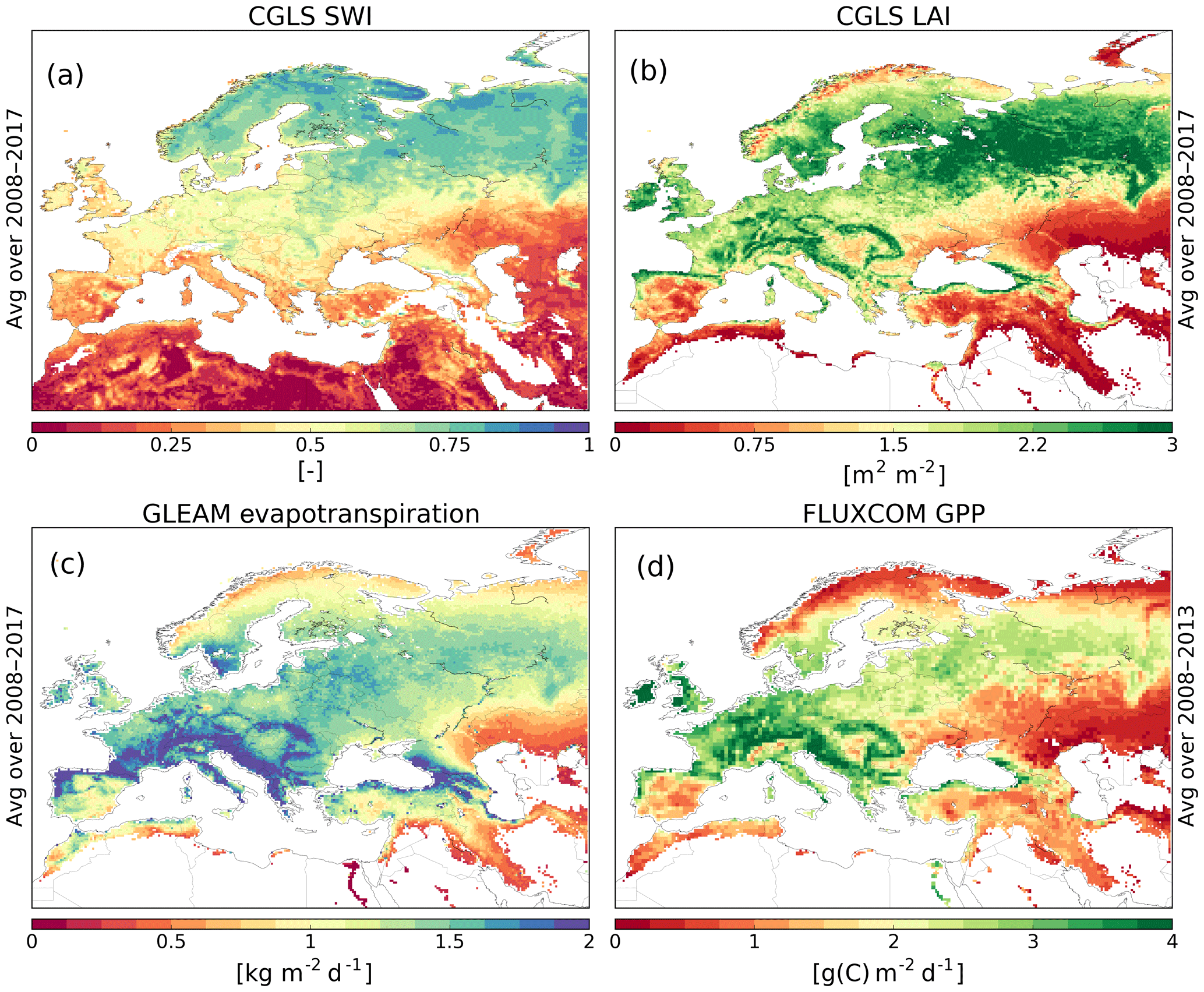
Figure 1 Satellite-derived products of the (a) original soil water index (SWI), (b) leaf area index (LAI), (c) evapotranspiration (ET) and (d) gross primary production (GPP) values. They are averaged over 2008–2017 for (a), (b) and (c) and over 2008–2013 for (d).

Prior to the assimilation, the SWI-001 product needs to be rescaled to the model climatology to avoid introducing any bias in the LDAS system (Reichle and Koster, 2004; Drusch et al., 2005). We apply a linear rescaling to SWI-001 to match the observation mean and variance to the mean and variance of the modelled soil moisture in the second layer of soil (1–4 cm). Introduced by Scipal et al. (2008), this rescaling gives in practice very similar results to CDF (cumulative distribution function) matching. The linear rescaling is performed on a seasonal basis (with a 3-month moving window). Draper et al. (2009) and Barbu et al. (2014) have highlighted the importance of allowing seasonal variability in the rescaling.

The GEOLAND2 version 1 LAI product is obtained through a neural network algorithm (Baret et al., 2013) transforming observations of reflectance from SPOT-VGT and PROBA-V satellites into LAI. This dataset is available every 10 d with the finest spatial resolution being 1 km. The GEOV1 LAI averaged over the 2008–2017 period can be seen in Fig. 1b.

Following Barbu et al. (2014), both observation datasets are interpolated on the model grid (0.25^∘ spatial resolution) where and when at least half of the observation grid points are available. As in previous LDAS-Monde studies, we use a 24 h assimilation window, and observations are assimilated at 09:00 UTC.

3.3 Validation datasets

We consider independent datasets of evapotranspiration (ET), gross primary production (GPP) and river discharges to assess the validity of our approach and measure the influence of the EnSRF on the improvement of LSV reanalyses.

Satellite-derived estimates of ET come from the GLEAM v3.3b product (Miralles et al., 2011; Martens et al., 2017). Daily estimates available for the period 1980–2018 at a 0.25^∘ spatial resolution are fully driven by satellite observations and, as such, are independent of LDAS-Monde estimates. Figure 1c displays GLEAM ET averaged over the period 2008–2017 considered for validation in this paper.

Observations of GPP are derived from the FLUXCOM project. This dataset is obtained by merging upscaled measurements from eddy-covariance flux towers and satellite observations using machine learning. More details can be found in Tramontana et al. (2016) and Jung et al. (2017). The FLUXCOM data are available at a 0.5^∘ spatial resolution on a monthly basis for the period 1982–2013. Figure 1d shows FLUXCOM GPP averaged over the period 2008–2013 considered for validation in this paper.

River discharge output data from the CTRIP river routing model are compared to daily streamflow data obtained from the Global Runoff Data Centre (https://www.bafg.de/GRDC, last access: 16 January 2020). Due to the low resolution of CTRIP (0.5^∘ spatial resolution), we only consider data for sub-basins with rather large drainage areas (greater than 10 000 km²) with a long enough time series (4 complete years or more over 2008–2017).

3.4 Experimental setup

To assess the impact of EnSRF on LSV reanalyses and compare its skill with the routinely used SEKF, we have run LDAS-Monde over the Euro-Mediterranean region (longitude from 11.5^∘ W to 62.5^∘ E, latitude from 25.0^∘ N to 75.5^∘ N) at a 0.25^∘ spatial resolution during the decade 2008–2017 for three different configurations: one model run without assimilation (i.e. open loop), one using the SEKF and another one using the EnSRF with a 20-member ensemble. This size of the ensemble is consistent with Fairbairn et al. (2015) and Carrera et al. (2015). All three configurations start from the same initial state obtained after spinning up ISBA–CTRIP 20 times over 2008. This provides an initial state for which the system has reached equilibrium.

For the SEKF configuration, the Jacobian matrix Eq. (5) is obtained by finite differences using perturbed model runs. Following Draper et al. (2009) and subsequent studies, perturbations are taken proportional to the dynamic range (difference between the volumetric field capacity w_fc and the wilting point w_wilt) for the soil moisture variable. In practice, perturbations for SM are set to ${\mathrm{10}}^{-\mathrm{4}}\times \left(w_{\mathrm{fc}}-w_{\mathrm{wilt}}\right)$. Regarding the fixed background error covariance, we prescribe a mean volumetric standard deviation (SD) of 0.04 m³ m⁻³ for SM in the second layer and 0.02 m³ m⁻³ for SM in deeper layers, both are then scaled by the dynamic range of SM. For LAI, perturbations are set to a fraction (0.001) of the modelled LAI following Rüdiger et al. (2010). LAI background error SD is set to 20 % of the LAI value for modelled values above 2.0 m² m⁻² and to a constant 0.4 m² m⁻² for modelled values below 2.0 m² m⁻². This SEKF configuration is the same as the one detailed in Albergel et al. (2017).

About the EnSRF configuration, the initial ensemble is obtained by perturbing the initial state using perturbations sampled from a multivariate Gaussian distribution with a zero mean and using the prescribed B covariance matrix used in the SEKF as the covariance matrix of that multivariate Gaussian distribution. Ensemble Kalman filters tend to underestimate variances and ensembles spreads. This brings about an artificially small spread leading ultimately to filter divergence if not counteracted. Hamill and Whitaker (2005) has shown that adding random perturbations to each ensemble member (additive inflation) at the start of each assimilation cycle can overcome this issue. It can also be used to represent model error. As in Fairbairn et al. (2015) we use time-correlated model errors using a first-order auto-regressive model. We prescribe an associated Gaussian noise with zero mean and an SD of λ(w_fc−w_wilt) for SM, with λ=0.5 for SM in layer 2 (1–4 cm depth), 0.2 for SM in layer 3 (4–10 cm depth), 0.05 for SM in layer 4 (10–20 cm depth) and 0.02 for SM in deeper layers. These values are in line with Fairbairn et al. (2015). For LAI, we prescribe a Gaussian noise with zero mean and an SD of 0.5 m^2 −2. We also fix the time correlation to 1 d for SM in the second layer and 3 d for SM in deeper layers. This is similar to the work of Reichle et al. (2002) and Mahfouf (2007). For LAI, a rather small 1-day time correlation has to be used in order to avoid a collapse of the ensemble during the winter season due to the LAI threshold in ISBA.

For both SEKF and EnSRF configurations, we follow previous LDAS-Monde studies and set SSM observational errors to 0.05 m³ m⁻³ scaled to the dynamic range and LAI observational errors to 20 % of the observed LAI values (see e.g Albergel et al., 2017; Leroux et al., 2018; Tall et al., 2019).

3.5 Evaluation strategy

As a check, we first verify that EnSRF estimates of SSM and LAI are closer to observations than their open-loop counterparts. We also compare the impact of EnSRF and SEKF on SM in layer 2 (1–4 cm depth; SM2) and LAI. This is achieved using scores such as biases, correlation coefficients (R), root mean square differences (RMSDs) and normalized root mean square differences (nRMSDs; RMSD divided by the averaged value of the studied variable).

The impact of assimilation on unobserved control variables (SM in deeper layers) is then assessed using a daily analysis increment. Moreover, we study the evolution of the ensemble correlations between unobserved and observed variables in the EnSRF configuration. They drive (as Jacobian values in the SEKF configuration) the influence of observations on unobserved control variables. We focus on SM in layer 4 (10–20 cm depth; SM4) and layer 6 (40–60 cm depth; SM6), as SM in layer 3 (4–10 cm depth) exhibits the same behaviour as SM4, and soil moisture in layer 5 (20–40 cm depth) and layer 7 (60–80 cm depth) have the same behaviour as SM6 (not shown).

Potential improvements in EnSRF and SEKF estimates of ET and GPP are measured using the same metrics as for SSM and LAI.

Finally the influence on river discharges for both DA approaches is measured by the Nash–Sutcliffe efficiency (NSE) score.

$$\begin{array}{}\text{(13)}& \mathrm{NSE}=\mathrm{1}-{\displaystyle \frac{{\sum }_{t=\mathrm{1}}^T(Q^{{\mathrm{s}}_t}-Q^{{\mathrm{o}}_t}{)}^{\mathrm{2}}}{{\sum }_{t=\mathrm{1}}^T(Q^{{\mathrm{o}}_t}-{\stackrel{\mathrm{‾}}{Q}}^{\mathrm{o}}{)}^{\mathrm{2}}}},\end{array}$$

where $Q^{{\mathrm{s}}_t}$ is the simulated or analysed river discharge at time t, $Q_t^{\mathrm{o}}$ is the observed river discharge at the same time and ${\stackrel{\mathrm{‾}}{Q}}^{\mathrm{o}}$ is the observed averaged river discharge. The NSE is a quantity between −∞ and 1. An NSE value of 1 means that the model or analysis perfectly matches observations. An NSE value of 0 means that the model or analysis has the same NSE as the observed averaged river discharge. Improvements or degradations caused by the SEKF or the EnSRF compared to the open loop is measured with the normalized information contribution index (NIC).

$$\begin{array}{}\text{(14)}& {\mathrm{NIC}}_{\mathrm{NSE}}=\mathrm{100}\times {\displaystyle \frac{{\mathrm{NSE}}_{\mathrm{analysis}}-{\mathrm{NSE}}_{\mathrm{model}}}{\mathrm{1}-{\mathrm{NSE}}_{\mathrm{model}}}}\end{array}$$

4 Results

4.1 Impact of assimilation on LAI

Figure 2 displays the open-loop, SEKF and EnSRF analyses and observed LAI 10 d time series averaged over Europe and the Mediterranean basin and spanning the period 2008–2017. It shows that the model simulation underestimates LAI compared to observations during winter and summer. The growing phase of vegetation occurs at a slower pace with averaged LAI reaching its maximum early August instead of late June to early July for observations. The senescence phase subsequently takes place later in the autumn compared to observations. Both DA systems efficiently correct model simulations for that latter phase. However, both SEKF and EnSRF fail to compensate for the slower LAI dynamics of the model during spring. This is in compliance with what Albergel et al. (2017) and Leroux et al. (2018) have observed over the Euro-Mediterranean region. During the growing phase, modelled LAI is more sensitive to atmospheric conditions than to initial LAI conditions. This implies that, while DA can artificially add LAI and biomass, its impact can be limited by the atmospheric forcing. During the senescence, LAI dynamics is driven by the rate of mortality, thus making DA more efficient.

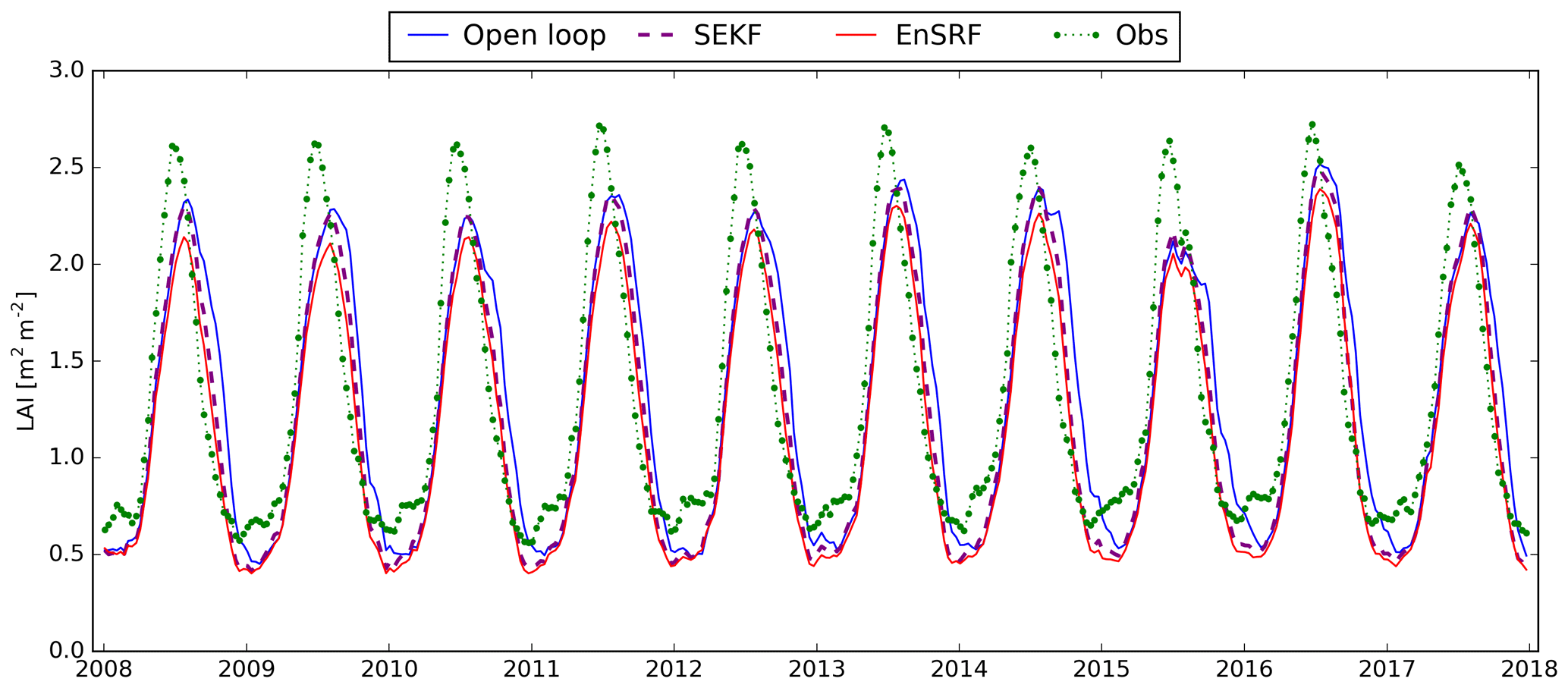
Figure 2 10 d time series of LAI averaged over the whole domain from the open loop (blue line), observations (green dots and dotted line) and analyses obtained with the SEKF (dashed purple line) and the EnSRF (red line) for the period 2008–2017.

As expected, both DA approaches produce estimates that are closer to the assimilated LAI observations than their open-loop counterpart. RMSDs are reduced from 0.880 m² m⁻² for the open loop to 0.671 m² m⁻² for SEKF and 0.694 m² m⁻² for EnSRF. Correlations with assimilated observations are increased from 0.593 for the model to 0.732 for SEKF and 0.723 for EnSRF. A full summary of statistics for LAI can be found in Table 1. We also note that the maximum LAI for EnSRF is smaller than the model or the SEKF maxima. The averaged bias for the open loop is rather small with −0.020 m² m⁻², but it hides a negative bias during winter and summer that is compensated for by a positive bias during autumn. DA approaches mostly correct the positive autumnal bias, thus making the averaged bias more negative, −0.116 m² m⁻² for the SEKF and −0.201 m² m⁻² for the EnSRF. The bias is more negative for the EnSRF than for the SEKF for every season. This is due in part to a systematic negative bias introduced by the EnSRF model perturbations. This bias can sometimes lead to degraded performances. As pointed out by Fairbairn et al. (2015), model perturbations can introduce a bias into the system in LDASs.

Table 1 Statistics (RMSD: root mean square difference, nRMSD: normalized RMSD, R: correlation and bias) between LDAS-Monde estimates (open loop, SEKF and EnSRF) and observations for CGLS SSM, CGLS LAI, GLEAM ET and FLUXCOM GPP averaged over the Euro-Mediterranean region for the period 2008–2017 (for SSM, LAI and ET) or 2008–2013 (for GPP).

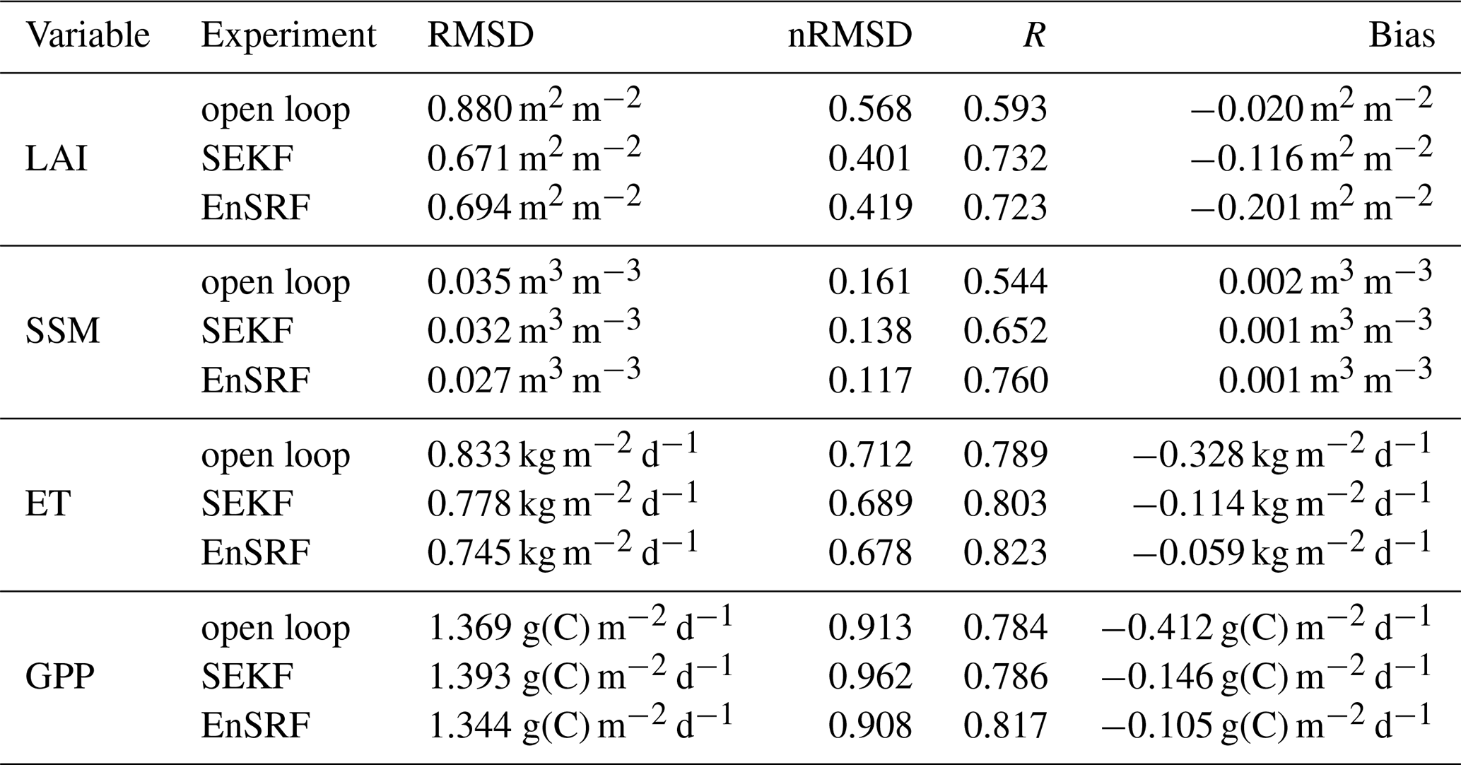
Figure 3 shows nRMSD calculated over 2008–2017 for the open loop (a) and the difference between nRMSD for the open loop and the estimates produced with SEKF (b) and EnSRF (c). On average nRMSD is reduced from 0.57 (open loop) to 0.42 (EnSRF) and 0.40 (SEKF). Both assimilation approaches display the same geographical patterns significantly reducing nRMSD over most parts of the Euro-Mediterranean region (in blue in Fig. 3). For example, roughly 20 % of the domain has an nRMSD reduced by 0.25. We note that the largest nRMSD reductions occur in places where nRMSD is large. The main differences between the two methods occur in Ireland, western Great Britain, northwest Spain, the Alps, Scandinavia and Arctic regions, where the SEKF shows a greater positive impact than EnSRF, the latter even providing slightly degraded estimates compared to the open loop for 3 % of the total domain (in red in Fig. 3c).

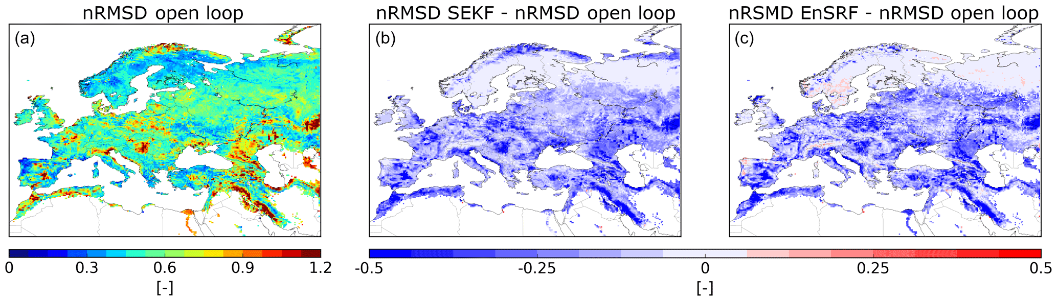
Figure 3 (a) Normalized RMSD (nRMSD) between observed LAI and its open-loop equivalent for the period 2008–2017 and the nRMSD difference between assimilation experiments (SEKF in b and EnSRF in c) and the open loop.

The geographical patterns identified in Fig. 3 can be explained in part by the type of vegetation covering grid cells. We investigate the impact of DA for each of the four main vegetation types encountered in the Euro-Mediterranean region: deciduous forests, coniferous forests, C₃ crops and grasslands. To that end, we consider only grid cells (GCs) in which at least 50 % of their surface is covered by one of these vegetation types. Figure 4 displays the spatial distribution of those grid cells: 1589 GCs for deciduous forests (5.7 % of the domain), 4223 GCs for coniferous forests (15.2 %), 1672 GCs for C₃ crops (6.0 %) and 1725 GCs for grasslands (6.2 %). We calculate the averaged seasonal RMSD for the open loop and SEKF and EnSRF analyses for the entire domain (Fig. 5a) and for each dominant vegetation type (Fig. 5b–e). The biggest impact of assimilating LAI occurs in autumn for deciduous forests (Fig. 5e). For example, RMSD is reduced from 2.69 m² m⁻² for the open loop to 1.72 m² m⁻² for the SEKF and 1.45 m² m⁻² for the EnSRF. For C₃ crops (Fig. 5c) both assimilation approaches reduce RMSD in a similar manner, the largest decrease happening between August and October. The SEKF and the EnSRF offer contrasting performances in the case of grasslands (Fig. 5d) as RMSDs are decreased by 0.18 m² m⁻² from the open-loop to SEKF estimates but by 0.09 m² m⁻² for EnSRF estimates. The largest RMSD reductions occur for both cases in April and September. This explains the reduced performance of the EnSRF compared to the SEKF over grasslands-dominated Ireland, western Great Britain and Arctic regions. For coniferous trees (Fig. 5b), the SEKF has a small positive impact on RMSDs, and the EnSRF has a slightly negative impact. This explains the rather poor performance of the EnSRF over Scandinavia. This also explains what happens in northwestern Spain and in the Alps. While not being dominated by one type of vegetation, coniferous trees and grasslands, the two types for which the EnSRF performs poorly, represent more than 70 % of the vegetation in those places.

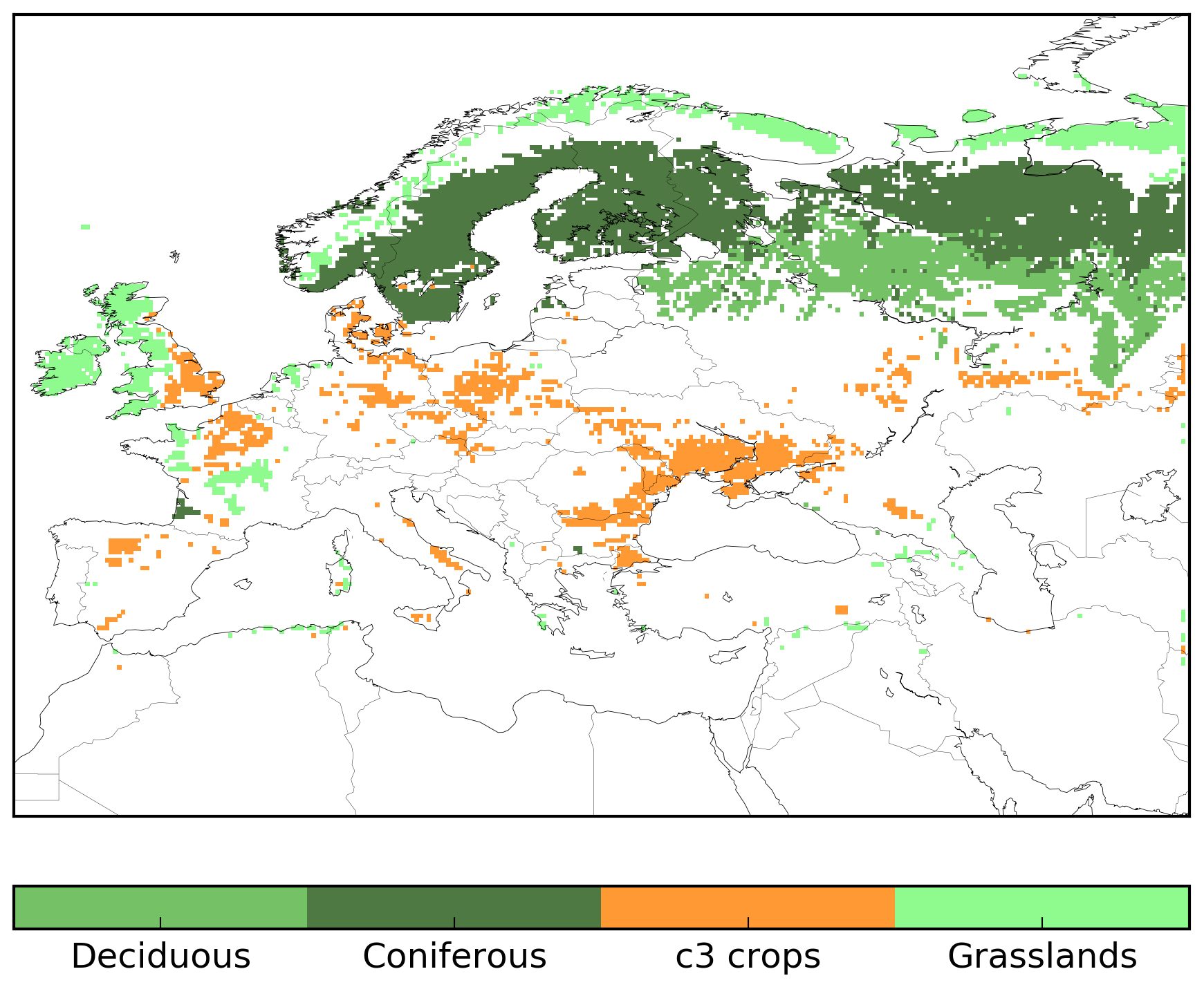
Figure 4 Grid cells of the domain where a vegetation type (or patch) is predominant (patch fraction above 50 %). Coniferous trees are dominant for around 15 % of the domain that has plants (dark green); deciduous broadleaved trees (green), C₃ crops (orange) and grasslands (light green) are in the majority for 6 % of the domain each.

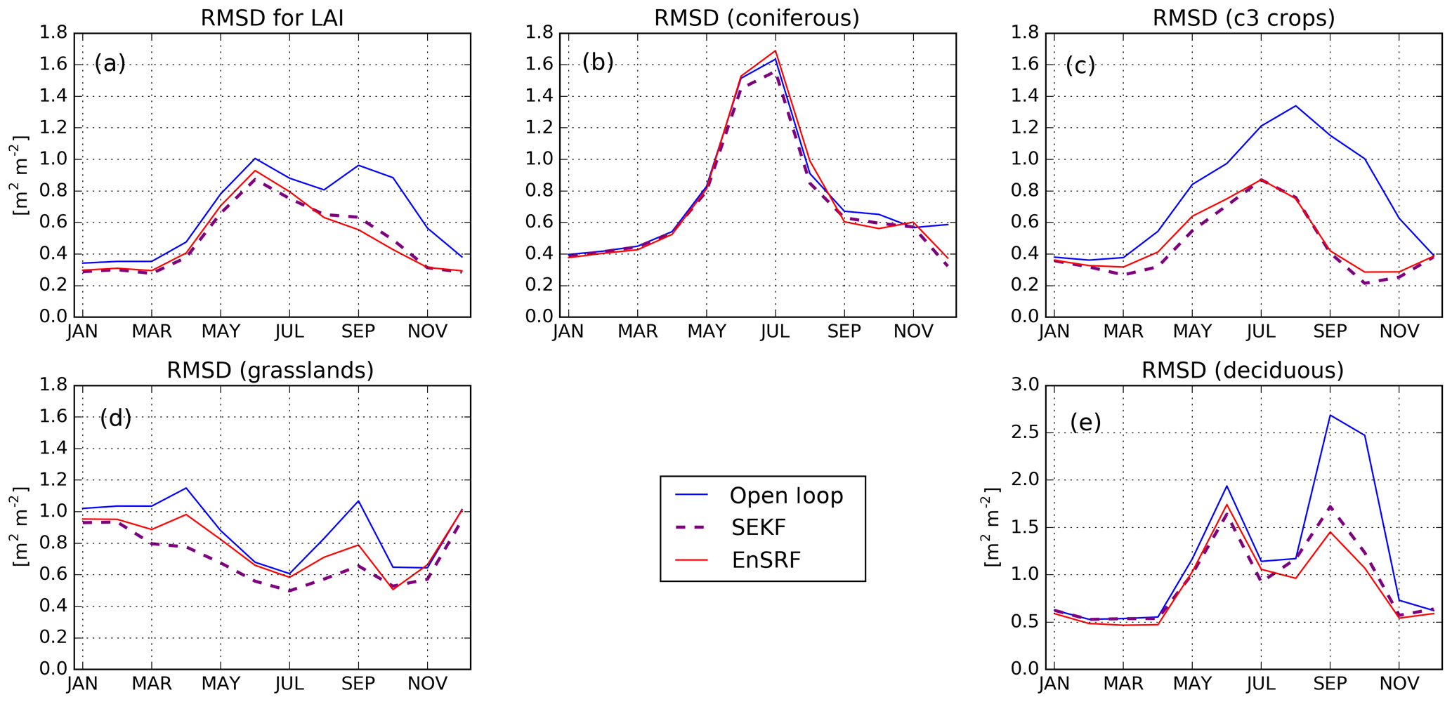
Figure 5 Seasonal RMSD between LAI from observations and the open loop (blue line), the SEKF analysis (dashed purple line) and the EnSRF analysis (red line) averaged over (a) the whole domain and grid cells where (b) coniferous trees, (c) C₃ crops, (d) grasslands and (e) deciduous broadleaved trees represent more than 50 % of plants for the period 2008–2017.

The scale of reduction in RMSD for EnSRF analyses is directly connected to estimated variances and standard deviations from the ensemble. The bigger the ensemble variances are, the larger the weight of observations in the DA system is. Figure 6 displays the seasonal evolution of ensemble standard deviations averaged over the whole domain and for grid cells dominated by one type of vegetation. Ensemble standard deviations are clearly larger in summer than in winter peaking in July for C₃ crops at 0.22 m² m⁻², in August for grasslands at 0.14 m² m⁻² and in September for coniferous forests at 0.07 m² m⁻². The maximum standard deviation is observed for deciduous forests and reaches 0.35 m² m⁻² also in September.

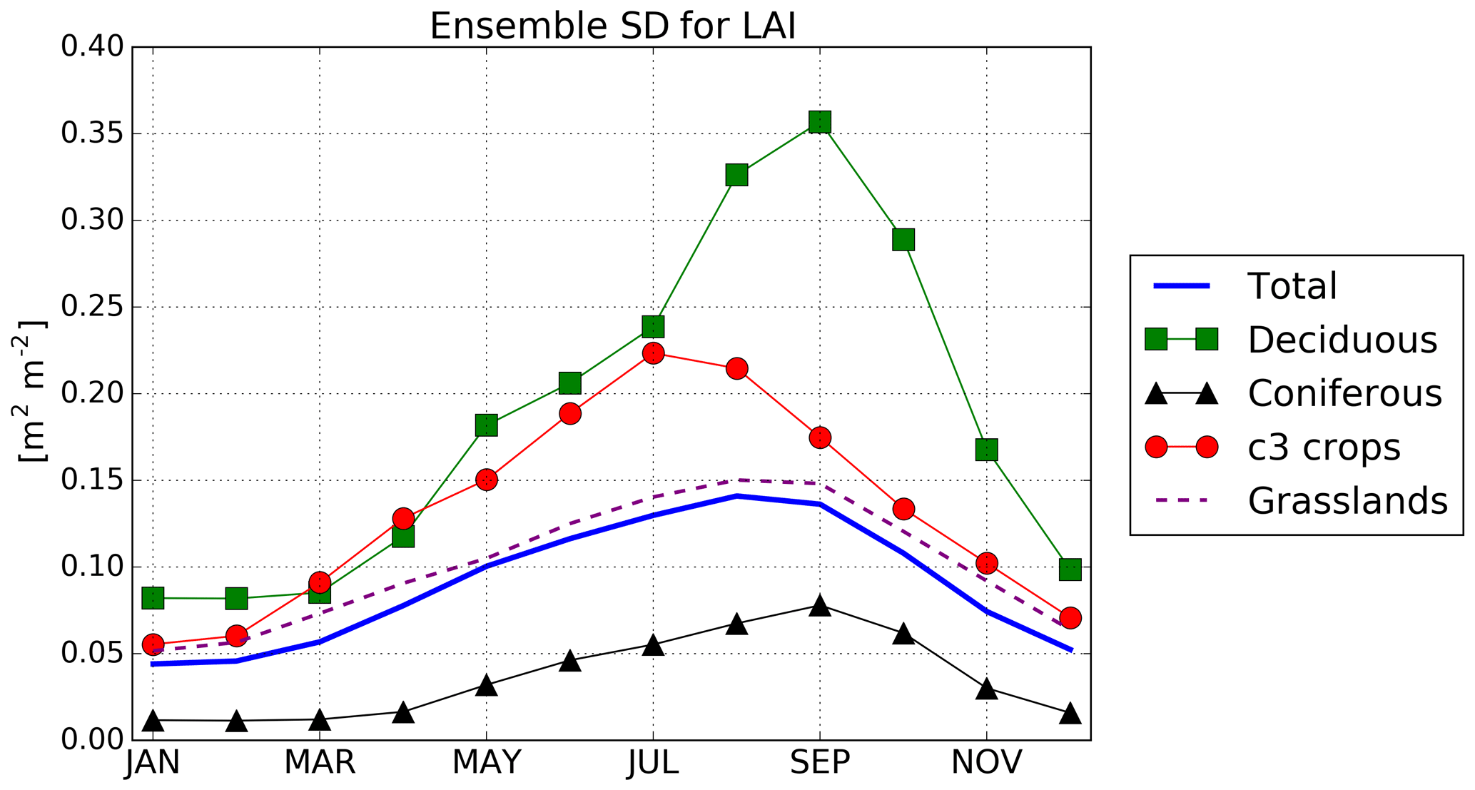
Figure 6 Seasonal standard deviation of the ensemble from the EnSRF averaged over the whole domain (thick blue line) and grid cells where deciduous broadleaved trees (green squares), coniferous trees (black triangles), C₃ crops (red circles) and grasslands (dashed purple line) represent the majority of plants for the period 2008–2017.

Standard deviations in the EnSRF relies heavily on the model perturbations. In the case of LAI, model perturbations applied to LAI in every vegetation patch are sampled from the same distribution. However, the behaviour of ensemble standard deviations varies greatly seasonally and for each type of vegetation. Standard deviations for coniferous trees are so low it leads to almost no impact of DA. Such behaviour can be explained by two caveats: first, ISBA-modelled LAI evolves over a prescribed threshold (1 m² m⁻² for coniferous forests, 0.3 m² m⁻² for other vegetation patches). Model perturbations can lead to LAI values below this threshold. To avoid model issues, estimated LAI is reset to that threshold when this is the case. It can lead to an artificially reduced ensemble standard deviation when modelled LAI is close to that threshold as in winter. Secondly, since LAI dynamics are smooth, reduced ensemble standard deviations due to the winter season still have an impact in spring through the ISBA LSM. An approach for model errors tailored for each vegetation patch could overcome the observed caveats.

4.2 Impact of assimilation on SSM

This section studies the impact of assimilating jointly LAI and SSM on estimated SSM. We firstly recall that observed SSM is derived from the SWI-001 satellite product and is matched to the model climatology of soil moisture in the second layer of soil (1–4 cm depth) using a seasonal linear rescaling. This means that assimilating observed SSM mostly corrects the short-term variability of estimated SSM and does not modify its climatological seasonal cycle. Results from either SEKF or EnSRF experiments are in line with this statement. For example, the bias between observed and estimated SSM remains, on average over 2008–2017, below 0.002 m³ m⁻³ over all the domain (see also Table 1 all the averaged scores with observed SSM).

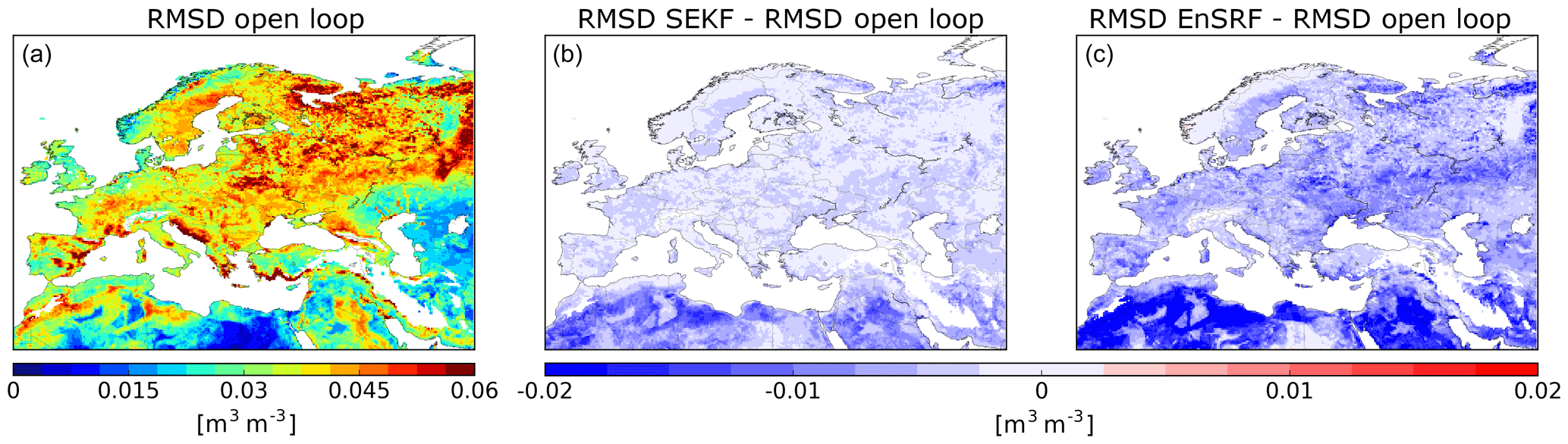
Figure 7 (a) Root mean square difference (RMSD) between observed (rescaled) SSM and its open-loop equivalent for the period 2008–2017 and RMSD difference between assimilation experiments (SEKF in b and EnSRF in c) and the open loop.

Figure 7 displays RMSD calculated over 2008–2017 for the open loop (a) and the difference between RMSD for the open loop and the estimates produced with SEKF (b) and EnSRF (c). On average, RMSD is reduced from 0.035 m³ m⁻³ (open loop) to 0.032 m³ m⁻³ (SEKF) and 0.027 m³ m⁻³ (EnSRF). RMSD for the open loop tends to be generally larger in wetter places than in drier places with the exception of southeastern Spain and parts of northern Africa where RMSDs can be larger than 0.050 m³ m⁻³. Both assimilation approaches significantly reduce RMSD in many places over the domain (in blue in Fig. 7b–c). The main reduction occurs for both approaches in the southern part of the Euro-Mediterranean region where grid cells consist of bare soil and bare rocks. In those places, vegetation is sparse, and SSM is the main source of information in assimilated observations, making its impact more straightforward. We also notice that the EnSRF tends to systematically produce estimates that are closer to observations than SEKF estimates. This is due to the model perturbations for the EnSRF and the prescribed background error covariance matrix in the SEKF. The prescribed model error for the EnSRF leads to ensembles with a bigger standard deviation than the one prescribed in the SEKF for SSM. This leads to a bigger weight to SSM observations in EnSRF than in SEKF, thus, making EnSRF estimates closer to SSM observations than SEKF estimates.

Assimilation also improves correlations with observed SSM from 0.544 for the open loop on average to 0.652 for SEKF and 0.760 for EnSRF. Figure 8 illustrates correlations for the open loop (a) and the difference between correlations for the open loop and SEKF (b) and EnSRF (c) outputs. From correlation results, similar conclusions are drawn as from RMSDs. In particular the main improvement occurs in northern Africa for both approaches. Finally we observe negative correlations between the open-loop and observed SSM (even with the seasonal linear rescaling) in arid places such as the Sahara and deserts in the Arabian Peninsula. This shows that the short-term variability of the observations is different from what we model with ISBA in this region. It raises the question of the quality of ISBA and/or SSM observations (after seasonal linear rescaling) in arid places. Stoffelen et al. (2017) have shown that observed SSM derived from scatterometers can have poor quality in arid places. Further studies of such aspects are beyond the scope of this paper.

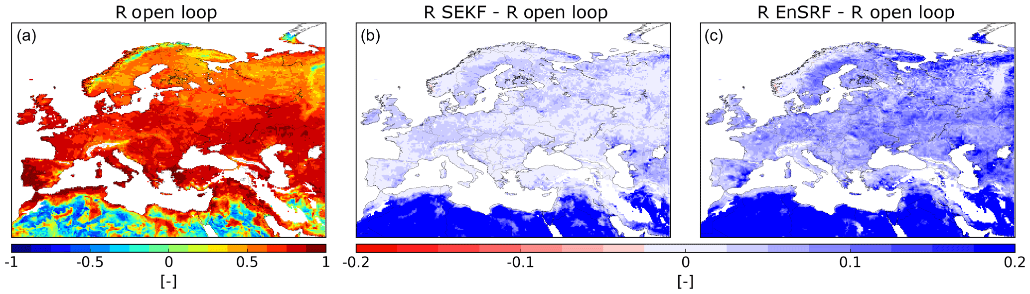
Figure 8 (a) Correlation (R) between observed (rescaled) SSM and its open-loop equivalent for the period 2008–2017 and R difference between assimilation experiments (SEKF in b and EnSRF in c) and the open loop.

4.3 Correlations between observed and unobserved control variables

Examining Jacobians in the SEKF has provided interesting insights into the sensitivity of SSM and LAI on soil moisture in deeper layers (see e.g. Albergel et al., 2017, for coverage of the Euro-Mediterranean region between 2000 and 2012). In the EnSRF, the Jacobian is replaced by correlations sampled from the ensemble covariance matrix. Figure 9 shows maps of correlations between soil moisture in layer 2 (1–4 cm depth; SM2, which is used as a proxy for SSM) and SM in layer 4 (10–20 cm depth; SM4) and layer 6 (40–60 cm depth; SM6) and correlations between LAI and SM2, SM4 and SM6. Correlations are averaged by season (December–January–February, March–April–May, June–July–August and September–October–November) over the whole period 2008–2017.

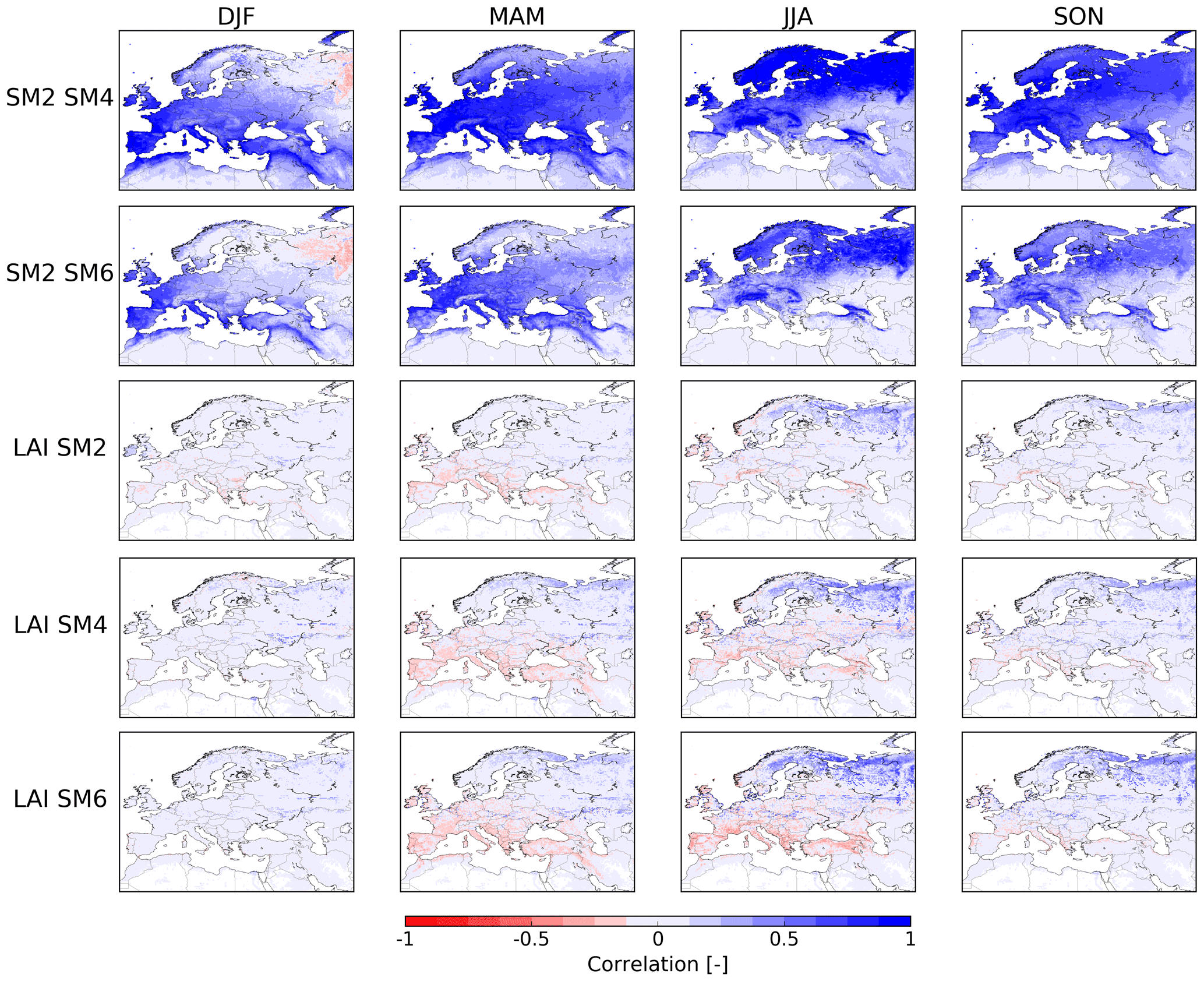
Figure 9 Correlation between the model variables sampled from ensembles and averaged seasonally (DJF: December–January–February, MAM: March–April–May, JJA: June–July–August and SON: September–October–November). From top to bottom: correlation between soil moisture in the second layer (1–4 cm; SM2) and the fourth layer (10–20 cm; SM4), between SM2 and soil moisture in the sixth layer (40–60 cm; SM6), between LAI and SM2, between LAI and SM4, and between LAI and SM6. Areas is blue exhibit positive correlations; areas in red exhibit anti-correlations.

The first two rows of Fig. 9 show the seasonal evolution of correlations between SM2 and SM4 and SM6. SM4 is highly correlated to SM2 (in blue), with R being above 0.5 for most places of the domain for each season. SM6 is also highly correlated to SM2, but it is to a lesser extent, meaning that correlations with SSM decrease in absolute value when we reach deeper soil layers. We also notice seasonal tendencies. For example, correlations with SM2 tend to be larger in western Europe during spring, while they reach their maximum during summer in Scandinavia. Negative correlations with SM2 (between −0.35 and −0.20) tend to appear during winter over Russia. It means that in those areas in winter, there is less liquid water in the surface when there is more liquid water in deeper layers. This is linked to snow and freezing as we only compare liquid soil moisture from the different layers of soil. We further notice that SM2 and SM6 are uncorrelated in summer over Spain and northern Africa. This decorrelation between surface and root-zone soil moisture occurs during very dry conditions, such as those which occurred in Spain and northern Africa during summer. The same phenomenon appears in very arid places such as in the Sahara. SM2 is not correlated to soil moisture in deeper layers such as SM4 or SM6 for each season. This implies that assimilating SSM in those areas will not modify soil moisture in deeper layers, as we will show in the next section.

The last three rows of Fig. 9 show the seasonal evolution of correlations between LAI and soil moisture in layers 2, 4 and 6. Soil moisture tends to be less correlated on average to LAI than to SSM; nevertheless the values reached are relatively large (between −0.5 and 0.5). It means that assimilating LAI has an impact on estimated soil moisture. In detail, correlations between LAI and SM6 are larger in absolute value than SM4 and SM2, meaning that LAI is more correlated to root-zone soil moisture than with SSM. We also observe seasonal geographical patterns. Positive correlations tend to appear in summer in northern Europe, where deciduous and coniferous forests are dominant, meaning more water in the soil leads to a greater LAI. On the contrary in spring and summer, negative correlations appear around the Mediterranean basin. This means a higher LAI leads to reduced soil moisture due to plant transpiration in part. Barbu et al. (2011) has already highlighted this kind of behaviour for Jacobians for grassland places in southwest France.

Overall conclusions drawn from correlations are in accordance with those derived from the analyses of SEKF Jacobians drawn in Albergel et al. (2017) over the Euro-Mediterranean region and Tall et al. (2019) over Burkina Faso. Nevertheless, we note that correlation can be influenced by the way we apply model error. Another type of model error, perturbing for example atmospheric forcing, may have led to different characteristics of the covariances between the ISBA variables.

4.4 Impact of assimilation on soil moisture in deeper layers

Figure 10 displays soil moisture for layers 4 and 6 averaged over 2008–2017 from the open loop (left) and the averaged difference with SEKF estimates (central panels) and EnSRF estimates (right). We observe that the SEKF and the EnSRF overall have averaged SM4 values similar to the open loop. The main difference occurs in northern Africa and in the Arabian Peninsula, where the soil is estimated wetter than in SEKF, with a difference reaching 0.02 m³ m⁻³. This disparity over arid regions in due solely to a wet bias introduced by model error. In those places, EnSRF cannot correct this bias using observations of SSM or LAI. In other places, EnSRF can correct the bias potentially introduced by the model perturbations to unobserved control variables through the help of correlations. We also identify greater EnSRF SM4 estimates over places such as Poland and Spain, but the difference with the open loop is always below 0.01 m³ m⁻³.

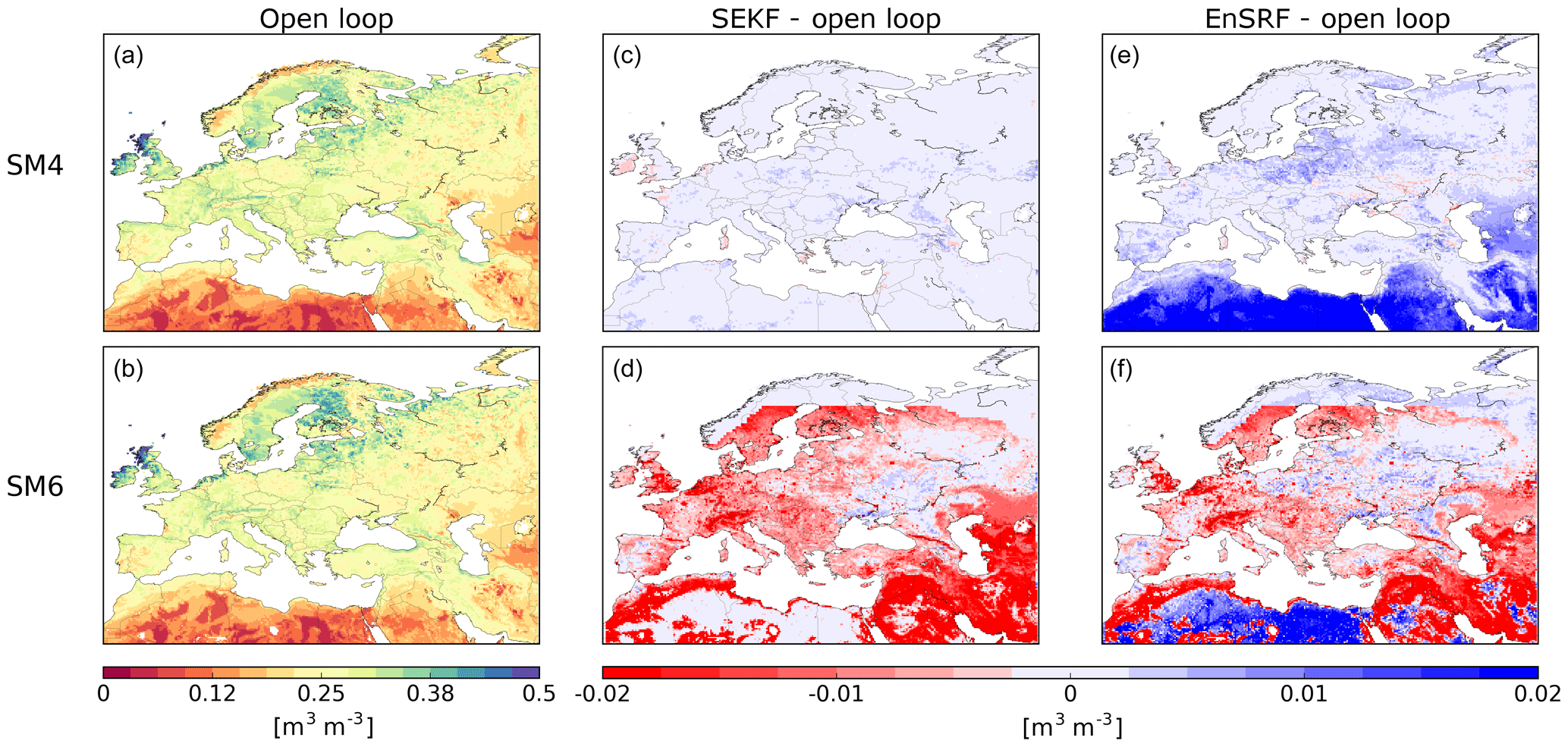
Figure 10 From left to right: averaged soil moisture for the open loop (fourth layer: 10–20 cm; SM4; sixth layer: 40–60 cm; SM6) over 2008–2017, averaged analysis impact for SEKF (c, d) and EnSRF (e, f).

Regarding SM6 estimates, both SEKF and EnSRF produce a drier soil layer than the model for most of the domain as shown in Fig. 10. We identify these patterns for every month without any seasonality (not shown). Also, EnSRF SM6 is wetter for regions where bare soil dominates in northern Africa than SM6 obtained with SEKF or the open loop. Again this is due solely to the wet bias introduced by model soil moisture perturbations as SM6 and SM2 are uncorrelated in those places. Then, we can observe for SM6 an abrupt change in the Arctic region for both SEKF and EnSRF compared to the open loop. This difference is due to modified hydraulic and thermal soil properties in ISBA for Arctic regions. This modification has been implemented by Decharme et al. (2016) in order to include a dependency on soil organic carbon content.

Figure 11 shows analysis increments in SM4 for SEKF (top row) and EnSRF (bottom row) for May, July and September. We see that increments in SM4 tend to be negative in May and September in most parts of the domain and positive in July, particularly in northern Europe for SEKF. The SM4 analyses increments for SEKF and EnSRF tend to be similar, except for arid regions. This makes the SM4 estimates less dependent on the data assimilation method.

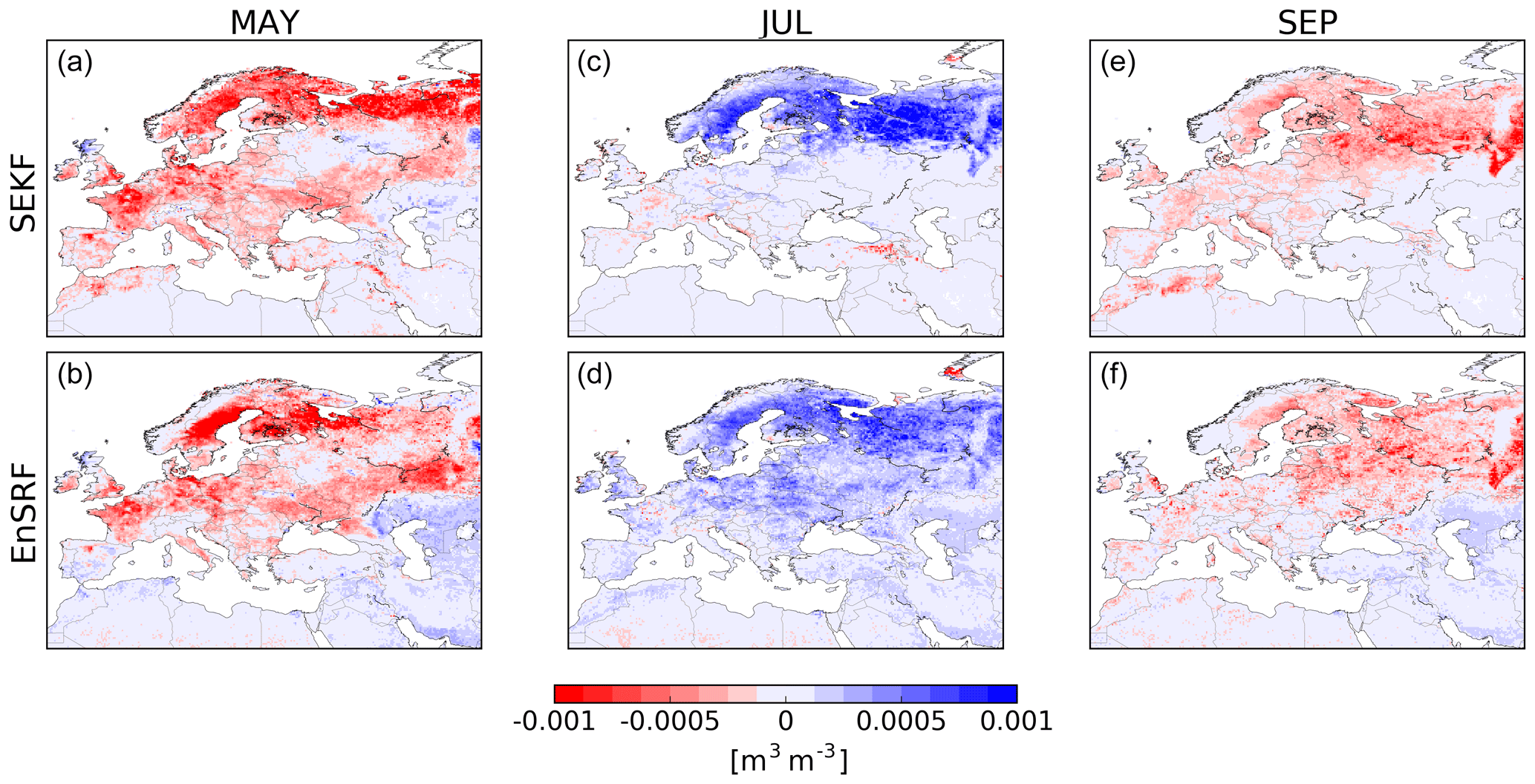
Figure 11 Averaged analysis increments for soil moisture in the fourth layer (10–20 cm; SM4) for SEKF and EnSRF for the months of May (a, b), July (c, d) and September (e, f).

For analysis increments for SM6, SEKF increments are close to zero for every season (not shown). This implies that the drier estimates are solely due to the joint effect of the ISBA LSM and the updated LAI and soil moisture near the surface. For EnSRF, this joint effect also occurs, but analysis increments are not negligible (−0.01 m³ m⁻³ for the biggest values). The EnSRF SM6 analysis increments compensate for the wet bias from model error (not shown) and lead to similar SM6 estimates as the SEKF in most places as shown previously.

Overall SEKF and EnSRF provide similar estimates for soil moisture in deeper layers for most places but not necessarily through the same mechanisms.

4.5 Evaluation using evapotranspiration and gross primary production

We now evaluate the performance of our data assimilation systems using independent satellite-based datasets of ET and GPP.

The open loop tends to underestimate ET leading to an averaged negative bias of −0.328 kg m⁻² d⁻¹ reaching −0.8 kg m⁻² d⁻¹ in June and July. Both SEKF and EnSRF reduce this bias to −0.114 and −0.059 kg m⁻² d⁻¹, respectively. More statistics on ET can be found in Table 1. Figure 12 displays correlations between the GLEAM dataset and open-loop estimates (a) and the difference between correlations for the open loop and the estimates produced with SEKF (b) and EnSRF (c). Overall the correlation is increased on average from 0.789 to 0.803 (SEKF) and 0.823 (EnSRF). EnSRF provides estimates that are more correlated with this independent dataset for almost all grid cells; it improves correlation (between 0.05 and 0.1) especially over Spain, northern Africa or around the Caspian Sea, where correlations between the open loop and GLEAM were poorer than for the rest of the domain, showing its positive impact on ET. Similar conclusions can be drawn from geographical patterns observed for RMSD and nRMSD (not shown; see Table 1 for averaged results).

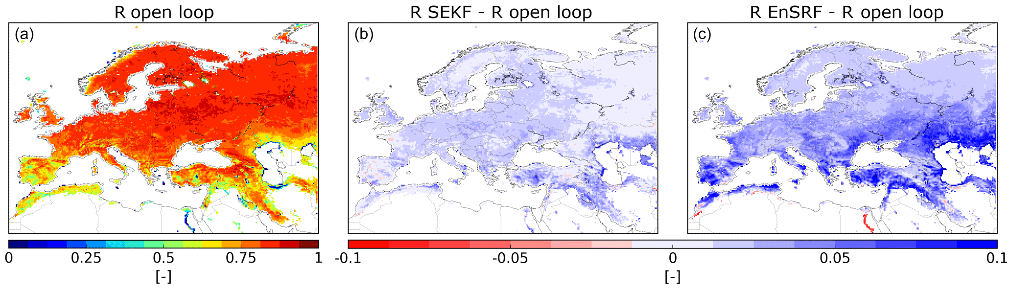
Figure 12 (a) Correlation (R) between observed GLEAM ET and its open-loop equivalent for the period 2008–2017 and R difference between assimilation experiments (SEKF in b and EnSRF in c) and the open loop.

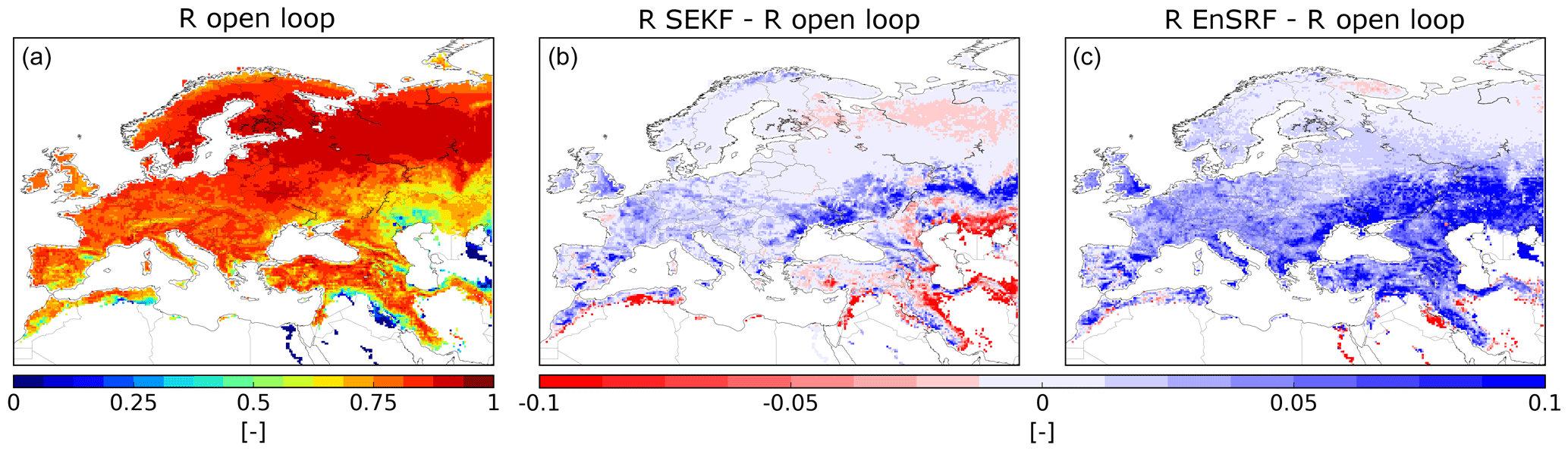
Figure 13 (a) Correlation (R) between observed FLUXCOM gross primary production and its open-loop equivalent for the period 2008–2013 and R difference between assimilation experiments (SEKF in b and EnSRF in c) and the open loop.

Figure 13 depicts the correlation between GPP from the FLUXCOM dataset and open-loop estimates (a) and the difference between correlations for the open loop and the estimates produced with SEKF (b) and EnSRF (c). As for ET, EnSRF provides GPP estimates that are more correlated to the FLUXCOM dataset than open-loop and SEKF estimates for almost everywhere, on average 0.817 compared to 0.784 for the model and 0.786 for SEKF. The biggest improvements are noticeable around the Caspian Sea (above 0.05), where correlations between the model and FLUXCOM GPP were poorer than for the rest of the domain. Also contrary to the SEKF, degradations are confined to only few places in Iraq, Iran and close to the Arctic Circle. Again similar conclusions can be drawn from geographical patterns observed for RMSD and nRMSD (not shown; see Table 1 for averaged results).

Overall the EnSRF exhibits moderate improvements for GPP and ET compared to SEKF.

4.6 Evaluation using river discharges

We limit our evaluation to 92 stations over Europe with a model NSE above −1. The NIC of EnSRF compared to the open loop is displayed for those stations in Fig. 14. Most stations are located in France and Germany. Blue circles denote a positive impact (above 3 %) of EnSRF on estimated river discharges; red circles denote a negative one (below −3 %); and grey diamonds denote a neutral impact (between −3 % and 3 %). A positive NIC is observed for 61 stations and a negative NIC for only 11 stations. The rest of the stations (20) showed a neutral impact. The largest NIC values are seen for German stations. Such a positive influence for EnSRF contrasts with the rather neutral effect of SEKF on river discharges. In compliance with previous studies (Albergel et al., 2017; Fairbairn et al., 2017), we observe a significantly positive NIC of SEKF for only 15 stations and a negative NIC for 3 stations (not shown).

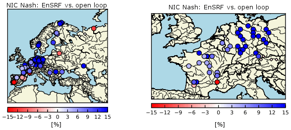
Figure 14 Normalized information contribution (NIC) index assessing the improvement of Nash–Sutcliffe efficiency indices for EnSRF river discharge estimates compared to open-loop counterparts. Blue circles denote a positive impact of DA; red circles denote a negative impact; and small diamonds denote a neutral impact.

The rather systematic improvement of EnSRF estimates compared to the open loop may be due in part to the assimilation of SSM and LAI. It may also be due in part to a bias added by the EnSRF ensemble formulation (as observed for other LSVs) that compensates for an existing bias due to the coupling between ISBA and CTRIP. Further investigations have to be conducted to explore this question. Moreover, a negative NIC is observed for most of the Spanish stations, where anthropogenic effects (irrigation, importance of dams, etc.) can potentially modify soil moisture, streamflow and river discharges (Milano et al. , 2013). Since CTRIP does not consider anthropogenic effects, this can explain poor performances of the LDAS–CTRIP system.

5 Discussion

5.1 Dealing with model errors in the LDAS-Monde EnSRF

As seen in the previous section, the quality of EnSRF estimates highly depends on the specified model error. We have seen that our system would benefit from a more tailored approach. One way that has been followed in the LDAS community is to use perturbed atmospheric forcings to generate more physical model perturbations and to obtain an ensemble whose covariances are more physically based. This can be done by either perturbing precipitations only (e.g. Fairbairn et al., 2015; Munier et al., 2015), operating a more complex system of perturbations that includes correlations between precipitation, or shortwave and longwave radiation (see among others Reichle et al., 2007; Liu et al., 2011; Kumar et al., 2014). Another possibility is to perturb land parameters such as the soil texture (Blyverket et al., 2019) or vegetation parameters. The main drawback of such approaches is that they tend to overcome underestimated ensemble variances by putting too much uncertainty on atmospheric forcings or model parameters that might be far better known than assumed. They can also induce a bias in model estimates (as shown by Fairbairn et al., 2015).

The model error in ensemble Kalman filters aims to compensate for insufficiencies of the model and forcings, but it is difficult to prescribe as it aims to compensate something we do not know. One way to curb this issue is to estimate model error. Dee (2005) describes a range of approaches to account for model biases in data assimilation systems. The last decade has also seen the development of techniques to estimate model error covariance matrices (see Tandeo et al., 2020, for a review of existing approaches). Approaches based on diagnostics developed in Desroziers et al. (2005) (Todling, 2015; Bowler, 2017) or on statistics of consecutive innovations (Berry et al., 2013; Harlim et al., 2014) seem affordable for LDASs from a computational point of view.

All these approaches help to estimate model deficiencies but do not necessarily provide the reasons for those caveats. For land surface models, they can come not only from possibly inadequate atmospheric or soil and vegetation parameters but also from inadequate model physics (missing processes, etc.). Finding the reasons for those is a complex task. An interesting step would be to assess the influence of atmospheric uncertainties on LSMs by using ensemble atmospheric forcings such as the 10-member atmospheric reanalysis included in ERA5 (available at a coarser spatial and temporal resolution though) or the 51 members of ECMWF ensemble medium-range forecasts. Such ideas have been explored over Spain in the case of multi-model and multi-forcing ensembles by Ehsan Bhulyan et al. (2019).

5.2 The question of 1-D or 3-D filtering

Both SEKF and EnSRF in this paper do not consider covariances between patches and between grid cells. However, those covariances are likely to exists. For example, each patch of a given grid cell is forced with the same atmospheric forcing, errors in the forcing would result in correlated errors for the state of each patch. The same thing could be said for the state of two neighbouring grid cells since errors in atmospheric reanalyses are spatially correlated (Hersbach et al., 2020). Including those covariances could be beneficial to LSV reanalyses.

By construction, the SEKF cannot include these covariances by itself. Indeed the SEKF relies on the ISBA land surface model to calculate covariances between variables by building the Jacobian matrix of the model. Since each patch of each grid cell of the model does not interact with the others, the Jacobian between two variables of different patches is zero. The same occurs for variables between different grid cells. Therefore, if we want to include covariances between patches or between grid cells, they have to be prescribed in the fixed background error covariance matrix.

On the contrary, ensemble Kalman filters can include this information automatically as estimated covariances are built from the ensemble, thus making EnKFs more flexible than the SEKF. In our case, that would lead to a single state vector containing LAI and SM in the various layers of soil of each patch, multiplied by around 12 for the size of this state. Fairbairn et al. (2015) and Carrera et al. (2015) have shown that LDASs can use a small ensemble to provide good LSV estimates without experiencing the traditional undersampling issues or spurious ensemble covariances. However, including covariances between patches or between grid cells would make undersampling and spurious covariances more likely to occur due to the increased size of the state vector. Nevertheless these two potential issues can be overcome. Inflation aims to compensate undersampling by artificially inflating the ensemble spread. Approaches have been built to estimate inflation (under the form of a multiplicative coefficient). Anderson (2009) has proposed to add inflation as a parameter in the control vector leading to inflation being updated at each EnKF analysis. Bauser et al. (2018) have successfully applied this approach to a soil hydrology problem. Other approaches based on consistency diagnostics developed by Desroziers et al. (2005) (Li et al., 2009; Miyoshi, 2011) or reformulated EnKFs (Bocquet, 2011; Bocquet and Sakov, 2012) have gained popularity.

Long-range spatial spurious covariances can be filtered out using localization procedures either by artificially reducing distant spurious correlation (Hamill et al., 2001; Houtekamer and Mitchell, 2001) or by assimilating observations locally (Ott et al., 2004); LDAS-Monde could be seen as an extreme application of the second approach because of the 1-D nature of the ISBA LSM. Localization procedures are very efficient and are routinely used for a wide range of applications.

Unfortunately, the problem of potentially spurious covariances between patches remains as we would need to fix a criterion to determine which covariance has to be reduced. Recently Farchi and Bocquet (2019) have proposed a localization procedure based on augmented ensembles. Such formulation allows for a covariance localization not based on spatial characteristics, and it could be used to include covariances between patches in the LDAS-Monde EnSRF.

6 Conclusions

In this paper, we have adapted the ensemble square root filter used by Fairbairn et al. (2015) to the context of the joint assimilation of surface soil moisture and leaf area index within LDAS-Monde. The validity of our approach has then be assessed over the Euro-Mediterranean region for the period 2008–2017 and compared to a simplified extended Kalman filter that is routinely used in LDAS-Monde. Results show that EnSRF provides estimates of LAI of a similar quality to SEKF. Estimated EnSRF surface soil moisture levels tend to get closer to observations than their SEKF counterparts. We have also examined the impact of EnSRF on controlled soil moisture for deeper soil layers. For soil moisture in near-surface layers (4–20 cm depth), analysis increments are similar for both approaches, but EnSRF estimates tend to be wetter especially for arid places due to a bias introduced by the model error perturbations. For deeper layers (20–80 cm depth), SEKF and EnSRF estimates of soil moisture are similar but are obtained through different mechanisms. While drier soil moisture in SEKF is obtained through the model by transferring information from updated soil moisture at or near the surface, the EnSRF produces soil moisture estimates partly because of the data assimilation routine itself, acting like a bias correction procedure for soil layers either near the surface or in the root zone to compensate for the wet model bias via the correlations between soil moisture in deeper layers and surface soil moisture and LAI. Finally, validation of our approach has been carried out using datasets of ET, GPP and river discharges, showing a moderate positive impact for ET and GPP, but it is a marked positive one for river discharges. This paper shows the potential of EnSRF within LDAS-Monde and constitutes a good basis for further developments.

One limitation of assimilating LAI is that LAI products are only available every 10 d (for CGLS products). This only allows for an update of LAI every 10 d, as the assimilation of surface soil moisture is found to have a negligible impact on the LAI analyses. LDAS-Monde would benefit from having observations linked to vegetation available every day. Lievens et al. (2017) and Shamambo et al. (2019) have shown that ASCAT radar backscatter coefficients can be linked to surface soil moisture and LAI (or vegetation optical depth) through a water cloud model. The development and the calibration of the water cloud model linking surface soil moisture and LAI to radar backscatter coefficient is currently under development at CNRM. Assimilating ASCAT radar backscatter coefficients would replace the assimilation of ASCAT-derived soil water indices. It would open the possibility of having access to daily indirect observations of LAI and improve LDAS-Monde daily updates of LAI and soil moisture.