Future shift in winter streamflow modulated by the internal variability of climate in southern Ontario

Fluvial systems in southern Ontario are regularly affected by widespread early-spring flood events primarily caused by rain-on-snow events. Recent studies have shown an increase in winter floods in this region due to increasing winter temperature and precipitation. Streamflow simulations are associated with uncertainties mainly due to the different scenarios of greenhouse gas emissions, global climate models (GCMs) or the choice of the hydrological model. The internal variability of climate, defined as the chaotic variability of atmospheric circulation due to natural internal processes within the climate system, is also a source of uncertainties to consider. Uncertainties of internal variability can be assessed using hydrological models fed by downscaled data of a global climate model large ensemble (GCM-LE), but GCM outputs have too coarse of a scale to be used in hydrological modeling. The Canadian Regional Climate Model Large Ensemble (CRCM5-LE), a 50-member ensemble downscaled from the Canadian Earth System Model version 2 Large Ensemble (CanESM2-LE), was developed to simulate local climate variability over northeastern North America under different future climate scenarios. In this study, CRCM5-LE temperature and precipitation projections under an RCP8.5 scenario were used as input in the Precipitation Runoff Modeling System (PRMS) to simulate streamflow at a near-future horizon (2026–2055) for four watersheds in southern Ontario. To investigate the role of the internal variability of climate in the modulation of streamflow, the 50 members were first grouped in classes of similar projected change in January–February streamflow and temperature and precipitation between 1961–1990 and 2026–2055. Then, the regional change in geopotential height (Z500) from CanESM2-LE was calculated for each class. Model simulations showed an average January–February increase in streamflow of 18 % (±8.7) in Big Creek, 30.5 % (±10.8) in Grand River, 29.8 % (±10.4) in Thames River and 31.2 % (±13.3) in Credit River. A total of 14 % of all ensemble members projected positive Z500 anomalies in North America's eastern coast enhancing rain, snowmelt and streamflow volume in January–February. For these members the increase of streamflow is expected to be as high as 31.6 % (±8.1) in Big Creek, 48.3 % (±11.1) in Grand River, 47 % (±9.6) in Thames River and 53.7 % (±15) in Credit River. Conversely, 14 % of the ensemble projected negative Z500 anomalies in North America's eastern coast and were associated with a much lower increase in streamflow: 8.3 % (±7.8) in Big Creek, 18.8 % (±5.8) in Grand River, 17.8 % (±6.4) in Thames River and 18.6 % (±6.5) in Credit River. These results provide important information to researchers, managers, policymakers and society about the expected ranges of increase in winter streamflow in a highly populated region of Canada, and they will help to explain how the internal variability of climate is expected to modulate the future streamflow in this region.

1 Introduction

An increasing concentration of atmospheric greenhouse gas (GHG) is projected to increase air temperature globally and modify the regional precipitation regimes (Hoegh-Guldberg et al., 2018). GHG-driven climate change is projected to impact watershed fluvial hydrological regimes especially in snow-dominated regions (Barnett et al., 2005) with serious implications for flood management and water resources (Hamlet and Lettenmaier, 2007; Wu et al., 2015).

The quantification of streamflow and other hydrological processes using hydrological models is becoming an active area of research in various regions of the world. However, the use of hydrological models to project the future hydrology is subject to uncertainties (Clark et al., 2016) that have recently been intensely investigated (Leng et al., 2016). Part of the uncertainties are associated with the projections of climate through the choice of the global climate model (GCM), the GHG emission scenario (Kour et al., 2016; Stephens et al., 2010) and the climate data downscaling method (Fowler et al., 2007; Schoof, 2013). In addition, the temporal evolution of temperature and precipitation, simulated by the GCMs, is modulated by the internal variability of climate due to inherently chaotic internal processes within the climate system (Deser et al., 2014; Lorenz, 1963). These uncertainties are cascading to the hydrological processes and streamflow (Lafaysse et al., 2014), and additional uncertainties are associated with the choice of the hydrological models (Boorman et al., 2007; Devia et al., 2015) and model calibration techniques (Khakbaz et al., 2012; Moriasi et al., 2007).

The uncertainties due to the internal climate variability is one of the biggest sources of uncertainty for hydrological projections of the early 21st century (Harding et al., 2012; Hawkins and Sutton, 2009; Lafaysse et al., 2014). The internal variability of climate is a cause of the hiatus observed in global warming in the 2000s (Dai et al., 2015) and is expected to mask the impact of human-induced climate change on precipitation (Rowell, 2012) and streamflow (Zhuan et al., 2018). To assess the contribution of the internal variability of climate in the overall climate change projection uncertainty, GCM large ensembles (GCM-LEs), based on small initial condition variations between members of the ensemble, have been used recently (Deser et al., 2014; Kay et al., 2015; Kumar et al., 2015). This method was used to investigate how these uncertainties are transferred to hydrological processes in large watersheds (Gelfan et al., 2015). However, such coarse-scale GCM data should be downscaled to be used in small watersheds (Fowler et al., 2007). Despite the fact that regional climate models are a computationally costly downscaling method (Lafaysse et al., 2014; Thompson et al., 2015), regional climate model large ensembles (RCM-LEs) offer the possibility to relate each member of an RCM to large-scale variability from GCM-LEs. Furthermore, RCM-LEs avoid additional and ambiguous sources of uncertainty caused by the statistical methods (Gelfan et al., 2015). One such dataset is the Canadian Regional Climate Model Large Ensemble (CRCM5-LE), a 50-member high-resolution (12 km grids) regional model ensemble dataset produced over northeastern North America, which was recently developed as part of the Quebec–Bavaria international collaboration on climate change project (ClimEx – Climate Change and Hydrological Extreme Events; Leduc et al., 2019).

In the literature, several studies have projected an increase in winter streamflow in the Great Lakes region due to earlier snowmelt and an increase in precipitation (Byun et al., 2019; Erler et al., 2018; Grillakis et al., 2011; Kuo et al., 2017), but the role of the internal variability of climate was the subject of very few studies. Large ensembles have been previously used as input in multiple hydrological models in the Au Saumon catchment in southern Quebec (Seiller and Anctil, 2014) and in the Grand River watershed in southern Ontario (Erler et al., 2018). However, these studies only used a few ensemble members, thus removing the possibility of assessing a large range of internal variability in the projections of future hydrological responses.

The main goal of this study is to explore the impact of the internal variability of climate in the projections of hydrologic processes and winter streamflow in major watersheds in southern Ontario in the Great Lakes region. The Great Lakes region contains ∼20 % of the world's unfrozen surface freshwater, while southern Ontario is home to one third of the Canadian population (Statistics Canada, 2016). The specific objectives of this study are to (i) project the future evolution of streamflow in four watersheds in southern Ontario, using the Precipitation Runoff Modeling System (PRMS) forced by a large 50-member ensemble (CRCM5-LE) under an Intergovernmental Panel on Climate Change (IPCC) RCP8.5 scenario and (ii) investigate the impact of the future projected changes in the regional atmospheric circulation on the hydrologic processes and winter streamflow in these watersheds.

2 Methods

2.1 Study area

Southern Ontario is a humid region according to the Köppen–Geiger climate classification (Kottek et al., 2006), with an average annual precipitation of 1000 mm. The precipitation is well distributed throughout the year, and about 200 mm falls as snow in the winter (Wang et al., 2015). The amount of rain and snow varies spatially due to the presence of the Great Lakes. In winter the amount of snow is enhanced close to Lake Huron and Georgian Bay by lake effects (Suriano and Leathers, 2017), while in summer the precipitation is lower near the lakes because the convection is inhibited (Scott and Huff, 1996). The region is characterized by a mixed flood regime with high flows generated by rain, snowmelt and rain-on-snow events occurring from late February to early April (Burn and Whitfield, 2015). These events are occurring earlier recently due to a higher contribution of rainfall to the overall winter precipitation (Burn and Whitfield, 2015).

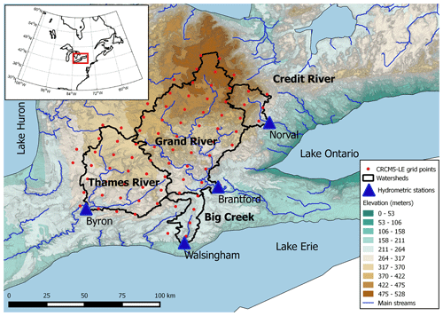
Figure 1 Location map of the four studied watersheds in southern Ontario. Elevation source: High Resolution Digital Elevation Model (HRDEM; Natural Resources Canada).

Table 1 Geomorphic, land use and soil characteristics of the four watersheds examined in this study.

Four watersheds (Big Creek, Credit River, Grand River and Thames River) were selected for this study considering their long hydrometric data and representation of the diversity of spatial scales, soil type and land use in this region (Fig. 1 and Table 1). Agriculture activity is the largest land use category in all four watersheds, covering more than 80 % of the entire surface in Big Creek, Thames River and Grand River. Credit River has the highest proportion of forest (32 %), mostly deciduous species. Several major urban areas are located in the study area: Brantford, Cambridge, Kitchener–Waterloo and Guelph in the Grand River watershed and London in the Thames River. Additional urban areas are located in the Credit River watershed in the vicinity of the Greater Toronto Area, while the Big Creek watershed contains the lowest proportion of urbanization (2 %). These watersheds also vary in soil type: sand predominates in Big Creek (79 %) and Credit River (43 %), but a large area of Credit River is covered by loamy soil (49 %). Grand River has almost an equal proportion of sand (30 %), loam (32 %) and clay (38 %), while Thames River contains more clay (39 %). The elevation is also highly variable with the highest altitudes in the northern parts of Grand River (531 m) and Credit River (521 m), while the lowest areas are located in the sand plains further south in Grand River (178 m) and Big Creek (179 m).

2.2 PRMS hydrological model

The Precipitation Runoff Modeling System (PRMS), a semi-distributed conceptual hydrological model developed by Leavesley et al. (1983), was applied in all four watersheds to simulate the future evolution of streamflow for each member of a large climate ensemble. PRMS is used in this study because it needs only basic daily forcing climate data (minimum and maximum temperature and precipitation). The advantage of using a model that needs only few data as input is that it reduces uncertainties from multiple variables and reduce the model's computational time. A drawback of using temperature is that energy balance is not physically represented. However, in an earlier study in the Big Creek watershed, PRMS represented the snow processes well (Champagne et al., 2019), showing that the use of temperature and precipitation is satisfactory to represent the snow processes in this region. Moreover, PRMS can be coupled with the MODFLOW (modular finite-difference flow model) groundwater model (GSFLOW) to study the interaction between surface and groundwater flow (Markstrom et al., 2008). While MODFLOW was not activated in this study, having PRMS set up in these watersheds will facilitate the use of GSFLOW in future studies. This model has been widely applied in watersheds that experience periodic snowfall (Dressler et al., 2006; Liao and Zhuang, 2017; Mastin et al., 2011; Surfleet et al., 2012; Teng et al., 2017, 2018).

The hydrological calculations in PRMS are based on physical laws and empirical relations between measured and estimated quantities. A series of hydrologic reservoirs (plant canopy interception, snowpack, soil zone and subsurface) is used in the model, and the water flowing between the reservoirs is computed for each of the grouped response units (GRUs). In this study the potential evapotranspiration was estimated using the Jensen–Haise formulation (Jensen and Haise, 1963). The interception was calculated separately for summer rain, winter rain and winter snow and was a function of the plant type. The separation between rainfall and snowfall was done by the snow module using temperature thresholds. If a day has a maximum temperature below 0 ^∘C, all precipitation of the day was considered as snow. If a day has a minimum temperature higher than 0 ^∘C and a maximum temperature higher than a threshold to calibrate, then all precipitation is considered rain. Mixed precipitation is computed when conditions are between these values. The snowpack dynamics are simulated through an estimate of energy and water dynamics. The energy available to melt the snow is based on the estimation of shortwave radiation, longwave radiation, convection and condensation. Shortwave solar radiation was estimated using a degree day method. Longwave radiation is the integration of the longwave radiation from the land cover and from the air depending on the emissivity of air. Convection and condensation are computed together as a function of temperature and a calibrated coefficient. Surface runoff due to infiltration excess (Hortonian runoff) is computed using the antecedent soil moisture content. The amount of water not contributing to Hortonian runoff is infiltrated and directed to the soil zone. The soil zone module computes transpiration, recharge to the groundwater reservoir and three components of the streamflow: saturation excess (Dunnian runoff), subsurface flow through soil cracks, animal borrows or leaf litter (fast interflow), and subsurface flow (slow interflow). These processes are described in more detail by Markstrom et al. (2015).

The model was set up for each watershed using Arcpy-GSFLOW, a series of ArcGIS scripts (Gardner et al., 2018). Arcpy-GSFLOW constructed GRUs as surface grid cells of 200 m² for Big Creek and Credit River watersheds and 400 m² for Grand River and Thames River. These latter two larger watersheds have coarser GRUs because the parametrization with Arcpy-GSFLOW is not functional with an excessive number of GRUs. An example of the GRU grid is shown for the southern part of Big Creek (Sect. S1 in the Supplement). Arcpy-GSFLOW calculated the physical characteristics of each GRU: elevation, slope and aspect were derived from the High Resolution Digital Elevation Model (HRDEM); the percentage of each land use type was derived from the Canadian Land Cover, Circa 2000 dataset (Natural Resources Canada, 2020) and used to calculate the rooting depth; and the available water content, saturated hydraulic conductivity, and percentage of sand and clay were estimated using the materials from the surficial geology of southern Ontario (Ontario Ministry of Energy, Northern Development and Mines). From these calculated characteristics, the spatialized parameters have been calculated at each GRU: the coefficients used to calculate slow interflow have been estimated using the saturated hydraulic conductivity and the slope. The maximum available water for plants was calculated using the available water content and the root depth and was used to estimate the total soil saturation. Finally, the linear coefficient used to route the water from the soil zone to the groundwater reservoir was estimated using the saturated hydraulic conductivity. The dominant land use type (bare soil, grassland, shrubs, coniferous trees or deciduous trees) and a single dominant soil type (sand, loam or clay) for each GRU were also estimated and used in some PRMS modules. Arcpy-GSFLOW was also used to define the stream network from HRDEM. The accumulation flow threshold was determined empirically by matching the streams with aerial photographs. We then estimated the water cascade between the GRUs and the stream network. The lakes represent very small areas of the watersheds and are therefore considered to have a negligible effect on streamflow. Control structures or dams were not taken into consideration in this study because of their limited impact on the 30-year average streamflow used in this study. The model was calibrated and validated using the regulated flow series. Therefore, the dam effect should be implicitly accounted for during the model calibration, and it is assumed that the reservoir levels will not change significantly in the future period.

Table 2 Parameter values after calibration. C: calibrated; GIS (geographic information system): estimated by Arcpy-GSFLOW; μ: GRU average. All parameters definitions can be found in Markstrom et al. (2015).

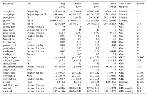
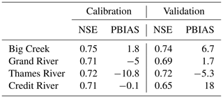
The spatialized parameters estimated by Arcpy-GSFLOW were modified during calibration while keeping their relative spatial variability. Other parameters were lumped to the entire watershed and were calibrated as well (Table 2). Model calibration was performed with a trial and error approach following three steps: (1) the calibration of the daily shortwave radiation parameters using satellite data (2002–2008) from Natural Resources Canada at 10 km resolution (Djebbar et al., 2012); (2) the potential evapotranspiration (PET) parameters adjusted against PET values estimated using the Thornthwaite method (Thornthwaite, 1948), and (3) calibration of 17 parameters using the normal root mean square error (NRMSE) between daily and monthly streamflow simulated by PRMS and daily and monthly observations measured at each watershed outlet (blue triangles in Fig. 1; Environment and Climate Change Canada Historical Hydrometric Data). A sensitivity analysis of the parameters in the Big Creek watershed (Supplement) shows that the infiltration to the soil zone is the most important process to accurately simulate the streamflow (smidx module). The available water threshold (soil_moist_max) as well as the travel time between stream segments (k_coef) are also important factors. For the snow module specifically, the convection–condensation energy coefficient (cecn) is the most sensitive (Sect. S3). The simulated streamflow was computed using precipitation, minimum temperature and maximum temperature from NRCANmet, the most commonly used dataset in Canada (Werner et al., 2019). The dataset was produced using station observation data from Environment and Climate Change Canada and Natural Resources Canada. The gridding at 10 km spatial resolution was accomplished using the Australian National University Spline (ANUSPLIN; McKenney et al., 2011). A total of 186 data points were necessary to cover the area of the four watersheds. For model calculations, each GRU used climate data from the closest NRCANmet grid point (Sect. S1). A warm-up period of 5 years was used (October 1984–September 1989) to remove any error due to initial conditions. Different simulations with a varying initialization period length were tested in the Big Creek watershed and showed that a period of 5 years was necessary for the hydrological model to forget the initial conditions of the reservoirs. The calibration period was between October 1989 and September 2008, and the years 2009 to 2013 were used as the validation period.

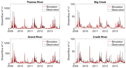
Figure 2 Daily observed (OBS) and simulated (CTL) streamflow during the validation period (2009–2013).

The best sets of parameters retained after calibration are shown in Table 2. The spatial variability of the parameters estimated for each of the GRUs can be found in the Supplement (Sect. S2). The Nash–Sutcliffe efficiency (NSE) values are always higher than 0.65 for both calibration and validation periods (Table 3), which is generally considered a good quantitative fit (Moriasi et al., 2007). A percent bias (PBIAS) between −15 % and +15 %, also considered a good fit, was reached in our study with the exception of Credit River for the validation period. Figure 2 shows the simulation and the observation of the daily streamflow in all four watersheds and visually confirms the goodness of fit for the simulation. The ability of the best set of parameters to recreate the snow depth in the Big Creek watershed was tested in a previous study (Champagne et al., 2019) and shows good agreement with the observations.

Table 3 Efficiency of the PRMS model for best-fit parameters.

2.3 Climate data projections

The set of parameters identified for each watershed during the calibration was used to simulate the future evolution of streamflow for each member of the Canadian Regional Climate Model Large Ensemble (CRCM5-LE). CRCM5-LE is a 50-member ensemble of climate change projections at 0.11^∘ (∼12 km) resolution available at 5 min time steps over northeastern North America (Leduc et al., 2019). Each member of CRCM5-LE was driven by 6-hourly atmospheric and oceanic fields from each member of the Canadian Earth System Model version 2 Large Ensemble (CanESM2-LE) at a 2.8^∘ (∼310 km) resolution (Fyfe et al., 2017; Sigmond et al., 2018). The downscaling from CanESM2-LE was performed using the Canadian Regional Climate Model (CRCM5 v3.3.3.1; Martynov et al., 2010; Šeparović et al., 2013), which was developed by the Centre ESCER (Centre pour l'étude et la simulation du climat à l'échelle régionale) at UQAM (Université du Québec à Montréal) with the collaboration of Environment and Climate Change Canada. The ensemble extends from the historical (1954–2005) to the projected (2006–2099) period forced with the RCP8.5 scenario (Meinshausen et al., 2011). The CRCM5-LE data grid points that were closest to NRCANmet data points were used in this study. Before their use in PRMS, modeled temperature and precipitation from CRCM5-LE were bias-corrected monthly against NRCANmet at each grid point over the historical period (1954–2005). The intensity distribution of temperature was corrected using a normal distribution. For precipitation, a two-step procedure was applied. The frequency distribution was first adjusted by truncating the modeled frequency. The truncated distribution of precipitation intensity was then corrected with a gamma distribution (Ines and Hansen, 2006). The bias correction method gives satisfactory results and was a necessary step before using CRCM5-LE in PRMS (Sect. S4). These bias correction values calculated from the historical period were applied at each CRCM5-LE grid point for the entire period of 1954–2099.

2.4 Agglomerative hierarchical clustering

Agglomerative hierarchical clustering (AHC) was used to classify all 50 members into classes of similar change of forcing CRCM5-LE meteorological conditions and streamflow simulated by PRMS. AHC is a bottom-up clustering approach where each observation (here members) starts as its own cluster and one pair of clusters is merged at each step, respecting a minimum change of total variance between each step (Ward, 1963). As a general concept, AHC first calculates the variance between each pair of observations. The pair with the lowest variance merges into a single class. In the next step, the pair of classes or pair of observations that would result in the smallest increase of total variance, compared to the previous step, is grouped together. This process is repeated until all classes of observations have been merged into a single class. In this study, AHC was applied first to the January–February normalized change in streamflow of all four watersheds and then to the average change of temperature and precipitation between the historical (1961–1990) and future (2026–2055) periods of the four watersheds. AHC was performed using January–February data because these months correspond to a large change in streamflow during the winter period. For precipitation and temperature, the period from 25 December to 22 February was used to account for the delay between weather conditions and streamflow at the outlet. A delay of 6 d showed the best correlation between the increase in temperature and precipitation and the increase in streamflow for all four watersheds. The number of classes to retain for the change of streamflow and the number of classes for the change of weather conditions correspond to the highest change in variance. The classification was used here to simplify the study of the connections between the future change in large-scale atmospheric circulation, local meteorological conditions and streamflow. This method using streamflow response classification rather than using a classification of climatological patterns was chosen because it focuses on the impact that can be used in other hydrological applications.

The future projection of atmospheric circulation for each class was analyzed using climate variables from CanESM2-LE with a geographical domain from 30 to 60^∘ N latitude and 100 to 50^∘ W longitude. Climate variables used for analysis included air temperature at 850 hPa level (850T), precipitation (PP), sea level pressure (SLP), geopotential height at 500 hPa (Z500) and surface winds. These climate variables were separated into internal and forcing contributors. The forcing contribution of the climate variables corresponds to the average change of all ensemble members between the historical period and future simulations. The internal contribution associated with each member was calculated by subtracting the original member data from the forcing contribution. This method was previously used by Deser et al. (2014) to assess the internal contribution of future change in temperature and precipitation in North America.

3 Results

3.1 Streamflow projections

Figure 3 shows the average daily streamflow volume and the number of high flows for all members for the historical (HIST) and future (2040s) periods. Observational streamflow measured at each watershed outlet (OBS) and the streamflow simulated by PRMS using observed temperature and precipitation from NRCANmet (CTL for control) are also shown for the historical period. A day is considered a high flow when the streamflow value is higher than the mean plus 3 times the standard deviation, based on observed streamflow. When at least 2 d in a row satisfy this condition, only 1 d of the series is considered as a high flow.

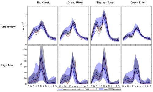
Figure 3 A 50-member range and average of streamflow and number high flows (Nb) for the historical and the 2040s periods.

In the historical period, average streamflow from OBS, CTL and the 50-member datasets followed similar annual cycles, with the first peak of the hydrological year occurring in November–December and the highest peak in March–April. By 2040, a clear peak in streamflow and the number of high-flow events is still modeled in March, but streamflow is more evenly distributed among winter months. This result suggests a shift from two maximal peaks to one winter peak by the mid-21st century. The largest increase in streamflow occurred in January–February, with a 50-member average increase reaching 18 % (±8.7) in Big Creek, 30.5 % (±10.8) in Grand River, 29.8 % (±10.4) in Thames River and 31.2 % (±13.3) in Credit River. All 50 members depict a streamflow increase in winter, but the simulated range of streamflow volume and the number of high flows is wide among the 50 different members.

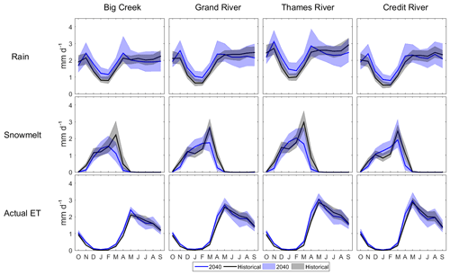
Figure 4 A 50-member range, average rain, snowmelt and actual ET amounts for the historical and the 2040s periods.

Daily rainfall, snowmelt, and actual evapotranspiration (ET) are also expected to change by the 2040s (Fig. 4). The amount of rain is simulated to consistently increase among the 50-member average in winter and early spring in all four watersheds. The 50-member average November–April increase in rainfall is about 29.7 % (±8.7) in Big Creek, 37.3 % (±10.3) in Grand River, 30.7 % (±8.6) in Thames River and 40.3 % (±11.7) in Credit River. In summer, PRMS simulates future average rainfall to decline between 5 % and 8.5 % depending on the watershed, but the direction of change is inconsistent between individual members. The amount of snowmelt is expected to shift from a high melt volume in March to a volume consistent throughout the winter. In March–April, snowmelt is expected to decline by 61.9 % (±11.2) in Big Creek, 52.2 % (±10.7) in Grand River, 60.5 % (±10.5) in Thames River and 42.8 % (±11.8) in Credit River, while in January–February, snowmelt is expected to increase by 10.2 % (±12.5) in Big Creek, 32.2 % (±12.7) in Grand River, 23.7 % (±11.7) in Thames River and 45.8 % (±16.1) in Credit River. Future ET will slightly increase for most months but decrease in summer.

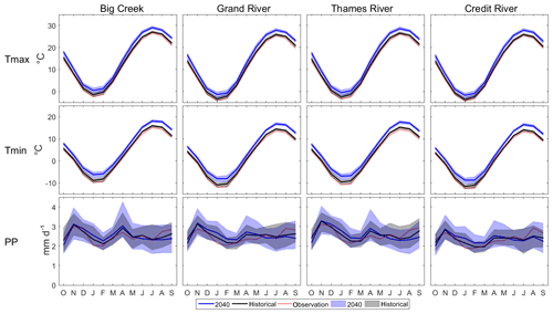
Figure 5 CRCM5 50-member range and average bias-corrected temperature and precipitation amounts for the historical and the 2040s periods, together with the observed temperature and precipitation.

Figure 5 shows the 50-member historical and projected bias-corrected temperature and precipitation for all four watersheds. Air temperature is shown to consistently increase for all months, while the range of precipitation amounts projected by the 50 members is wider compared to the change in temperature. On average, simulated precipitation increases in November–April and decreases in June–September.

3.2 January–February streamflow projections variability

The 50 members of the ensemble were classified first in classes of similar January–February streamflow change between the historical period and 2040s using AHC as described in Methods. The number of classes to retain was determined using a dendrogram (Fig. 6a). The dendrogram shows the cumulative total intraclass variance of normalized streamflow for the successive merging, from the first merging that uses all members at the bottom of the diagram to the last merging creating a single class at the top (Fig. 6a). The highest vertical distance between two successive merging in the y axis corresponds to the change in number of classes affected by the highest intraclass variance increase. The number of weather classes was identified using the same method (Fig. 6b). Three streamflow classes (HiQ, MoQ and LoQ for high, medium and low increase of streamflow; Fig. 6a) and four weather classes (HiPT, MoPT, LoPT and HiT; Fig. 6b) correspond to the classes merged right before the highest change in variance. Three of the weather classes (HiPT, MoPT and LoPT) show a gradient from high to low increase for both precipitation and temperature, while one weather class shows a high increase in temperature but low increase in precipitation (HiT; Fig. 6c). The labels “high” and “low” are not referring to absolute values but correspond to a higher or lower increase in streamflow and temperature or precipitation relative to the other members.

Figure 6 (a–b) Results of the agglomerative hierarchical clustering (AHC) for (a) the normalized change of streamflow (Q) and (b) normalized change of average temperature (T) and precipitation (PP). Colored numbers represent Q classes in panels (a) and (b). (c) Four-watershed average change of streamflow (Q) (colors) with respect to the average change of PP and T. Large hollow circles represent the four weather classes.

Table 4 Class members, percentage of the ensemble in the class and average January–February percentage increase of streamflow between the historical and the 2040s periods. The term in parenthesis indicates the standard deviation when the class has more than two members.

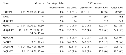
The streamflow and weather classes were then aggregated, grouping the members that are in the same streamflow and weather classes, giving a total of nine classes (Table 4). The increase in streamflow is similar between watersheds with the exception of Big Creek depicting a lower change. In Big Creek the classes corresponding to HiQ have an average increase of between 25 % and 32 %; MoQ increases between 18 % and 24 %; and LoQ increases between 8 % and 14 %. In the three other watersheds, HiQ depicts an average increase of between 39 % and 54 %; MoQ increases between 28 % and 36 %; and LoQ increases between 18 % and 24 % (Table 4). The interclass variability is also generally consistent between watersheds with the exception of Big Creek, where the classes HiQHiT and LoQHiT show comparatively low streamflow increases as compared to other classes (Table 4).

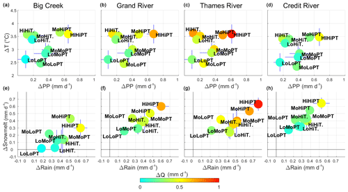
Figure 7 Change of streamflow (colors) with respect to changes of daily temperature and precipitation amount (a–d) and snowmelt and rain amounts (e–h) between the historical and the 2040s periods in January–February.

Table 4 emphasizes that despite a similar change in precipitation and temperature, the streamflow varies greatly between classes. Figure 7 shows scatterplots of the average change of the streamflow to the average change of precipitation, temperature, snowmelt and rain between the historical period and the 2040s period for all nine classes shown in Table 4. The HiQHiPT and LoQLoPT classes are associated with the highest (lowest) increases of streamflow due to high (low) increases of snowmelt and rain (Fig. 7). The larger increase in rain and snowmelt for HiQHiPT members is likely due a larger warming and an increase in precipitation. MoQLoPT demonstrates a larger increase in simulated streamflow compared to LoQLoPT, which is likely due to a larger increase of precipitation amounts despite lower warming. MoQLoPT is especially larger than LoQLoPT in terms of snowmelt, suggesting more snowfall for MoQLoPT members. The three weather classes associated with a large increase of temperature only (HiT) depict a moderate increase of rain and snowmelt suggesting that these members increase the rain-to-snow ratio and accelerate the snowmelt. LoQHiT also shows a strong warming but a low increase of snowmelt, explaining the low increase in streamflow (Fig. 7). Lastly, MoQMoPT has a higher increase in both rainfall and snowmelt compared to LoQMoPT, but both classes demonstrate a similar change of precipitation and temperature. These results suggest that alternative factors than average change in temperature and precipitation could explain the change in rainfall, snowmelt and streamflow in January–February. These factors will be described in Sect. 3.4 and discussed in Sect. 4.4. Lastly, the main visual difference between watersheds was a lower increase of snowmelt expected in Big Creek.

3.3 Atmospheric circulation and streamflow projections

The 50-member average change of temperature and precipitation between the historical period and the 2040s is shown in Fig. 8. An increase of air temperature at 850 hPa (T850) and geopotential height at 500 hPa (Z500) is expected to occur within the entire domain with a stronger gradient closer to the Arctic (Fig. 8c). Precipitation is also simulated to increase by the 2040s throughout the domain, while SLP is expected to decrease (Fig. 8d). In the region close to the Great Lakes, the magnitude of warming and variability between members is higher on the northern shorelines as compared to the open water and shorelines south of the Great Lakes (Fig. 8a). Precipitation increases is also projected to be higher on land and on the eastern side of the Great Lakes and toward the Atlantic coast (Fig. 8b and d).

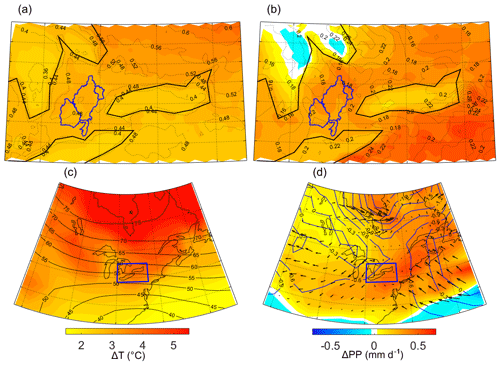
Figure 8 A 50-member ensemble average change of atmospheric conditions between the historical and the 2040s periods in January–February for (a) CRCM5-LE average surface temperature (shade) and standard deviation (black lines); (b) CRCM5-LE average daily precipitation (shade) and standard deviation (black lines); (c) CanESM2-LE T850 (shade) and Z500 (black lines); and (d) CanESM2-LE daily precipitation (shade), SLP (blue lines) and wind (vectors).

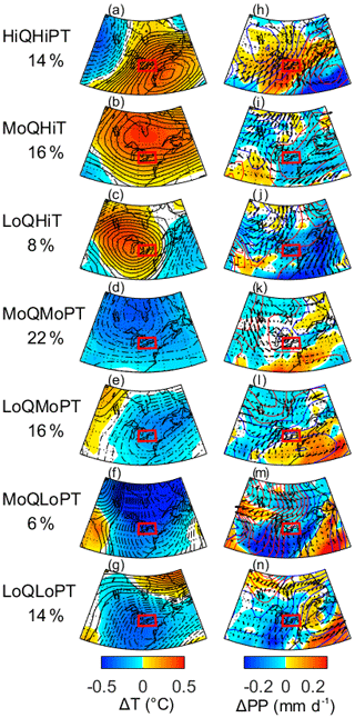
The internal contribution of each CanESM2-LE member to the change of climate variables was averaged for each class (Fig. 9). The class HiQHiPT is projected to be associated with positive change anomalies of temperature, precipitation and southwesterly winds between high-pressure anomalies in the east and low-pressure anomalies on the western side of the domain (Fig. 9a and h). LoQLoPT has opposite pressure gradient anomalies and is the only class that shows negative precipitation and temperature change anomalies occurring simultaneously (Fig. 9g and n). LoQMoPT demonstrates a pattern similar to LoQLoPT, but the negative pressure anomalies are attenuated, and the precipitation increase is higher (Fig. 9e and l). MoQHiT and LoQHiT are characterized by positive temperature and pressure change anomalies over southern Ontario, while MoQMoPT and MoQLoPT have an opposite pattern.

Figure 9 Class average internal contribution of (a–g) T850 (shade) and Z500 (black lines, in intervals of 1 m) and (h–n) precipitation (shade), SLP (lines, in intervals of 0.1 Pa) and wind (vectors) to the 50-member average change between the historical and the 2040s periods in January–February.

3.4 Antecedent conditions and streamflow

Factors alternative to January–February atmospheric conditions are also examined that may help to explain the January–February evolution of streamflow between the historical and the future periods. Figure 10 shows the change of precipitation amount in November–December, groundwater flow in January–February and amount of snowpack water equivalent for the first and the last day of the January–February period.

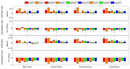
Figure 10 Class average (bars) and standard deviation (hatches) of the change between the historical and the 2040s periods of precipitation amount (mm) in November–December, snowpack amount (mm water equivalent – Weq) on 25 December, groundwater (GW) flow in January–February and snowpack amount (mm water equivalent – Weq) on 23 February.

November–December precipitation is projected to increase for all classes, but a large intraclass and interclass variability is shown. The classes HiHiPT, HiHiT, MoHiT and the two LoPT weather classes visually show a higher increase of November–December precipitation as compared to the other classes. The amount of snowpack water equivalent at the beginning of the January–February period is expected to decrease with low variability between the classes but with a large intraclass variability (Fig. 10). The snowpack at the end of January–February is expected to decrease significantly for all classes with a low intraclass variability. The groundwater flow visually shows a lower increase in Big Creek compared to the other watersheds, likely due to a lower overall increase in streamflow.

4 Discussion

4.1 Historical simulations

The observed seasonal cycle of streamflow was visually well reproduced by the simulated CTL and ensemble data for the historical period (1961–1990; Fig. 3). However, the simulated streamflow from CTL and the ensemble overestimated streamflow between November and February in the Thames River and Big Creek watersheds. The overestimation is stronger in January for the ensemble, which can be attributed to an overestimation of precipitation (Fig. 5). Winter overestimation was previously reported for the Grand River watershed (Erler et al., 2018) and was attributed to the lack of ponding or frozen-soil process representation in the model. Similarly, the version of PRMS used in our study did not represent the ponding and frozen-soil processes. However, a comparison of the observed streamflow during frozen- and non-frozen-soil periods in the Big Creek watershed showed a small difference (figure not shown), suggesting a small impact of frozen soil on the streamflow in this region. Moreover, the streamflow simulations using NRCANmet data performed well in Grand River (Fig. 3). These results suggest that factors other than the hydrological model are likely responsible for the discrepancies in Thames River and Big Creek. The quality of NRCANmet observations could also be a source of uncertainty. The ANUSPLIN method, used by NRCANmet to interpolate the station-based observations, generally overestimates precipitation in this region (Newlands et al., 2011). Despite these biases, NRCANmet is among the most widely used gridded dataset in Canada (Werner et al., 2019), and the use of NRCANmet to simulate snow processes was satisfactory in the Big Creek watershed (Champagne et al., 2019). The observed streamflow itself can also be affected by measurement uncertainty during ice conditions and especially an overestimation of the discharge. The validation of simulations using other variables such as evapotranspiration or soil moisture would be beneficial to improve the confidence in the results. Evapotranspiration from CRCM5-LE was not available for this work but could be investigated in future works.

4.2 Increase in streamflow amplified or attenuated by Z500 anomalies

Despite the discrepancies highlighted in the last section, the results show a clear increase of streamflow in January–February (Fig. 3) which has been previously simulated for other watersheds in the Great Lakes region (Byun et al., 2019; Erler et al., 2018; Grillakis et al., 2011; Kuo et al., 2017). January–February streamflow increases will likely be caused by temperature and precipitation increases (Figs. 5 and 8) that causes rain and snowmelt amounts to rise (Fig. 4). Grillakis et al. (2011) used several hydrological models in a small catchment close to Lake Ontario and projected streamflow increases due to rainfall increases in January and snowmelt increases in February. In our study we found an increase of rain and snowmelt for both months (Fig. 4). The future increase of January–February rain and snowmelt can be associated with the warming simulated by CanESM2-LE (Fig. 8). This warming has a similar amplitude compared to other CMIP5 (Coupled Model Intercomparison Project) model projections forced with the same RCP8.5 scenario (Zhang et al., 2019). An increase in January–February precipitation, projected in a large part of the domain (Fig. 8), is also similar to other climate models simulations (Zhang et al., 2019). Precipitation increase between Lake Ontario and Lake Erie and the eastern coast (Fig. 8) is not expected by the CMIP5 multimodel projections and is likely inherent to CanESM2-LE. This precipitation pattern is probably associated with stronger winds from the eastern coast (Atlantic Ocean) due to a higher-pressure decrease on land (Fig. 8).

The 50 members produce a variable increase of streamflow (Fig. 3), which is likely due to the variability in atmospheric circulation (Fig. 9). A total of 14 % of the ensemble showed a high increase of streamflow simultaneously with high geopotential height anomalies near the eastern coast and southerly winds through the Great Lakes region (Table 4 and Fig. 9a and h). Anomalies of high geopotential height located in the eastern United States have been previously found to be responsible for more precipitation and higher temperature in the Great Lakes region in winter (Mallakpour and Villarini, 2016; Thiombiano et al., 2017), thereby increasing the streamflow and high-flow events (Bradbury et al., 2002; Mallakpour and Villarini, 2016). A total of 14 % of the ensemble corresponds to the opposite pattern, with anomalies of low geopotential height on the eastern coast and anomalies of northern winds (Fig. 9g and n). These atmospheric conditions will attenuate the warming and precipitation amounts and will therefore be associated with a lower increase of streamflow (Table 4 and Fig. 7). A total of 6 % of the ensemble (Class MoQLoPT) shows a low warming but a moderate increase in precipitation and snowmelt (Figs. 7 and 9f and m), suggesting snowfall enhancement. The anomalies of northwestern winds associated with this class (Fig. 9f and m) could enhance snowfall in this region through lake effect snow (Suriano and Leathers, 2017). Another 16 % of the ensemble shows a moderate increase in streamflow associated with a strong warming (MoQHiT) which may be driven by anomalies of high geopotential height on the Great Lakes (Fig. 9b and i). This pattern drove moderate increases of snowmelt and the rain-to-snow ratio associated with strong warming (Figs. 7, 9b and i). Correspondence between high geopotential height and high temperature on the Great Lakes in winter have been previously reported (Ning and Bradley, 2015). Ning and Bradley (2015) suggested that the high geopotential anomalies on the Great Lakes prevent the polar jet stream and the cold air masses from entering the region.

4.3 Consistency in the weather classes

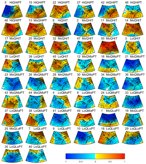
The weather classes are associated with specific trends in atmospheric conditions (Fig. 9) but are composed from an average of members that have their own atmospheric signature despite a similar impact on local conditions. Changes in Z500 and T850 anomalies for each member are depicted in Fig. 11 to investigate the atmospheric variability between members. The members that comprise classes HiPT show a large increase in Z500 anomalies on the eastern coast consistently for six members, while for two members (13 and 48) the high increase in Z500 anomalies is centered north from the Great Lakes. Eight members of the class LoPT show strong Z500 decrease on the eastern coast, but in two members (1 and 10) the decline is rather centered on the northern side of the Great Lakes. HiT generally shows a Z500 increase centered on the Great Lakes, but 4 of the 13 members depict a different pattern (2, 20, 31 and 47). Finally, members from MoPT generally show a decrease in Z500, but we observe a high diversity in the change of circulation patterns. Members from MoPT depict a lower Z500 gradient compared to other classes, suggesting a lower contribution of the internal variability of climate to the total change in atmospheric conditions (Fig. 11). These results suggest a large variability in atmospheric circulation change between members of the same ensemble with some members showing very unique change in atmospheric circulation. Despite differences of the atmospheric anomalies between members predicting similar local weather, the class method used in this study gives a good probabilistic overview of how the change in regional atmospheric anomalies will impact local weather.

Figure 11 Internal change of T850 (shade) and Z500 (black lines, interval 2 m) between the historical and the 2040s periods in January–February for each member.

4.4 Lag between atmospheric circulation shifts, local climate conditions and streamflow

Results show that interclass variability in the increase of January–February streamflow is mostly due to temperature and precipitation variability in the same months. The members with the highest increase in January–February precipitation and temperature (HiPT) are the members associated with the highest January–February streamflow increases, except for MoQHiPT (Table 4). The members associated with the lowest increase in precipitation and temperature (LoPT) show the lowest streamflow increase (LoQLoPT). Three other members of LoPT are associated with higher streamflow increase (MoQLoPT), which can be due to more precipitation and snowfall despite a lower warming (Fig. 7).

Within the other two weather classes, HiT and MoPT, a similar change in January–February weather conditions translates to a large range of streamflow projections. These discrepancies between the evolution of weather conditions and streamflow volume in January–February can be associated with a delay between weather conditions and streamflow. To account for the routing delay between rain and snowmelt events and streamflow observed at the outlet, our analyses used a lag time of 6 d between the precipitation and temperature and the streamflow. Any remaining delay between weather conditions and streamflow could occur due to the snowpack remaining from the previous months. Figure 10 shows a low variability between all MoPT members and all HiT members in terms of change in starting snowpack volume, suggesting a low impact of snowpack remaining at the end of December on change in January–February streamflow. Meanwhile, snowpack remaining at the end of January–February decreases at a higher rate for MoQMoPT members as compared to LoQMoPT members and for MoQHiT members compared to LoQHiT members (Fig. 10), which may be associated with a higher increase in snowmelt (Fig. 7). However, these two classes show very similar changes of temperature and precipitation (Fig. 7), suggesting that average weather change obscures intraseasonal variability change. For example, if more snow falls in the second half of February and the temperature stays below the freezing point, this snow is likely to melt in March and is therefore not counted in the January–February streamflow.

The discrepancy between the change in weather conditions and streamflow can also be due to groundwater recharge–discharge variability. The lower streamflow increase in LoQHiT is, for example, associated simultaneously with a lower increase in groundwater flow and a lower increase in November–December precipitation amount (Fig. 10). A correlation close to 0.7 between the 50-member November–December change in precipitation amount and the January–February change in groundwater flow confirms the connection between fall precipitation and winter groundwater flow. The processes connecting fall precipitation and winter groundwater will need further investigation with the help of a coupled surface and groundwater model, such as GSFLOW, for instance (Markstrom et al., 2015). These results emphasize the possible role of processes delaying the streamflow (i.e., snowpack and groundwater) and the need to also study the succession of different atmospheric patterns in the months before the January–February modulation of streamflow.

4.5 Spatial variability of streamflow change modulation

The changes in the amount of rain and snowmelt between the historical period and the 2040s are visually similar for three of the watersheds (Fig. 7). The Big Creek watershed is distinctly different, as it shows a lower snowmelt contribution to streamflow (Fig. 7). This suggests a thinner snowpack available for melting in this watershed, as it is situated in the southern part of the study area near Lake Erie and experiences the mildest winters (Fig. 5). In this watershed, the snowmelt volume is expected to increase only slightly in January (Fig. 4). The increase in snowmelt is also expected to occur only in January for Thames River, while the increase will be stronger in February for Grand River and Credit River. A similar south–north pattern is observed in previous studies. A high increase in streamflow in December and January followed by a decrease in streamflow in February was simulated for the Canard watershed near Lake Erie (Rahman et al., 2012), while this shift is expected to occur between February and March further north near Lake Ontario (Grillakis et al., 2011; Sultana and Coulibaly, 2011) or Lake Simcoe (Kuo et al., 2017; Oni et al., 2014). These results suggest that the winter increase in streamflow is expected to be lower in the warmest watersheds classically situated further south, in lowlands and close to the Great Lakes. In these watersheds the snowpack was already reduced in the historical period, and the further warming is not expected to increase the snowmelt contribution to the streamflow. However, similar to previous studies in southern Ontario, the reduced snowpack is not projected to decrease the streamflow in winter because the winter precipitation is also projected to increase as suggested in the majority of the climate models (Zhang et al., 2019).

5 Conclusion

This study used a 50-member ensemble of regional climate data, forced with the IPCC RCP8.5 scenario, as input in the PRMS hydrological model to show how the internal variability of climate is transferred to the near-future winter (January–February) projections of streamflow in four diverse watersheds in southern Ontario, Great Lakes region. An agglomerative hierarchical clustering method was used to construct classes of similar change in temperature, precipitation and streamflow and define streamflow change probabilities and associated regional atmospheric drivers. First, the results showed that all members of the ensemble were associated with a January–February increase in streamflow between 1961–1990 and 2026–2055, with an average increase of 18 % (±8.7) in Big Creek, 30.5 % (±10.8) in Grand River, 29.8 % (±10.4) in Thames River and 31.2 % (±13.3) in Credit River. This streamflow increase is due to a strong warming trend and an increase in precipitation projected by the IPCC RCP8.5 scenario. Second, the results suggested that the future increase of temperature and precipitation in January–February will be modulated by the internal variability of climate with implications for hydrological processes. Specifically, our study showed that

• i.

  One class of CRCM5-LE members, representing 14 % of all ensemble members, depicted an amplification in the future average streamflow. The average streamflow change for this class will be as high as +31.6 % (±8.1) in Big Creek, +48.3 % (±11.1) in Grand River, +47 % (±9.6) in Thames River and +53.7 % (±15) in Credit River. This amplification will be due to rainfall and snowmelt enhancement associated with the development of high-pressure anomalies on the eastern coast of North America.

• ii.

  The opposite pattern, associated with anomalous low pressure on the eastern coast of North America, showed an attenuation in average streamflow. This class depicted a future change in streamflow of only +8.3 % (±7.8) in Big Creek, +18.8 % (±5.8) in Grand River, +17.8 % (±6.4) in Thames River and +18.6 % (±6.5) in Credit River.

• iii.

  Two other classes representing another 24 % of all ensemble members showed a moderate attenuation in streamflow increase with +12.7 % (±3.6) in Big Creek, +22.3 % (±3.3) in Grand River, +23 % (±2.3) in Thames River and +21.1 % (±6) in Credit River. This attenuation might occur due to low November–December precipitation and low January–February snow accumulation and melting.

• iv.

  Almost half of all ensemble members showed a change in temperature and precipitation close to the 50-member average and showed a small contribution of the internal variability of climate to the projected variability of streamflow.

These results focusing on average change of atmospheric conditions cannot be applied to high flows, mostly driven by the day-to-day variability of atmospheric circulation. The use of the same regional ensemble together with a classification of daily atmospheric fields would be useful to assess the future projections of high flows and flood regimes in the region. Despite a large number of regional climate simulations used here to drive a hydrological model, the results are derived from a single model chain (CanESM2, CRCM5 and PRMS). As a result, this ensemble does not consider other important sources of uncertainty from the emission scenario and model structure. Future studies could use other global climate models and different scenarios and can be extended to the end of the 21st century. Other hydrological models could also be used to increase the confidence regarding the projections of hydrological processes. This work is important to assess the natural variability of the hydrological projections and help society to be prepared for a large range of future changes in flooding regimes.