Linking economic and social factors to peak flows in an agricultural watershed using socio-hydrologic modeling

Hydrologic modeling studies most often represent humans through predefined actions and fail to account for human responses under changing hydrologic conditions. By treating both human and hydrologic systems as co-evolving, we build a socio-hydrological model that combines an agent-based model (ABM) with a semi-distributed hydrologic model. The curve number method is used to clearly illustrate the impacts of land cover changes resulting from decisions made by two different agent types. Aiming to reduce flooding, a city agent pays farmer agents to convert land into conservation. Farmer agents decide how to allocate land between conservation and production based on factors related to profits, past land use, and willingness. The model is implemented for a watershed representative of the mixed agricultural/small urban area land use found in Iowa, USA. In this preliminary study, we simulate scenarios of crop yields, crop prices, and conservation subsidies along with varied farmer parameters that illustrate the effects of human system variables on peak discharges. High corn prices lead to a decrease in conservation land from historical levels; consequently, mean peak discharge increases by 6 %, creating greater potential for downstream flooding within the watershed. However, when corn prices are low and the watershed is characterized by a conservation-minded farmer population, mean peak discharge is reduced by 3 %. Overall, changes in mean peak discharge, which is representative of farmer land use decisions, are most sensitive to changes in crop prices as opposed to yields or conservation subsidies.

1 Introduction

Humans change the water cycle through actions that affect physical and chemical aspects of the landscape, and these changes occur from global to local scales and over varying time periods (Vorosmarty and Sahagian, 2000). Despite their significant impacts to the landscape, humans remain the most poorly represented variables in hydrologic models (Sivapalan et al., 2012). Land cover and land use are commonly treated as fixed in time in many hydrologic models through the use of static parameters. When made dynamic, landscape change is often limited to predefined scenarios that are developed without consideration of how economics, local culture, or climate may combine to influence land use decisions. For example, the field of integrated water resources management (IWRM), which attempts to explore the interactions between humans and water, typically uses “scenario-based” approaches (Savenije and Van der Zaag, 2008). While scenario-based studies allow for the quantification of the impacts of a management decision on the hydrologic system, there are significant limitations (Elshafei et al., 2014; Sivapalan et al., 2012). Human and environmental systems are highly coupled: feedbacks from one system create stress on the other system, which, in turn, affects the behavior of the first system. Therefore, representing management decisions as predetermined will not reproduce the real-world variability that may arise as a result of complex feedbacks between the human system and the physical system.

Arguments have emerged in the hydrological sciences and water resources systems analysis (WRSA) fields for modeling in which humans and the environment are treated as co-evolving (e.g., Di Baldassarre et al., 2013; Brown et al., 2015; Montanari, 2015; Rosengrant et al., 2002; Sivapalan et al., 2012; Sivapalan and Blöschl, 2015; Wainwright, 2008). In this way, models can account for disturbances to natural systems by humans and simultaneously assess physical processes and economic and social issues. In the hydrologic literature, two approaches have been used to simulate coupled human and natural systems: a classic top-down approach and a bottom-up approach using agent-based modeling (ABM). In the first approach, all aspects of the human system are represented through a set of parameterized differential equations (e.g., Di Baldassarre et al., 2013; Elshafei et al., 2014; Viglione et al., 2014). For example, Elshafei et al. (2014) characterizes the population dynamics, economics, and sensitivity of the human population to hydrologic change through differential equations to simulate the coupled dynamics of the human and hydrologic systems in an agricultural watershed. In contrast, the ABM approach consists of a set of algorithms that encapsulate the behaviors of agents and their interactions within a defined system, where agents can represent individuals, groups, companies, or countries (Axelrod and Tesfatsion, 2006; Borrill and Tesfatsion, 2011; Parunak et al., 1998). System agents can range from passive members with no cognitive function to individual and group decision-makers with sophisticated learning and communication capabilities. The ABM approach has several advantages over the traditional top-down approach (Bonabeau, 2002). Agent-based models are able to capture emergent phenomenon that result from interactions between individual entities. In addition, simulating individual entities through ABM provides for a more natural description of a system in contrast to developing differential equations that capture the behavior of the system as a whole. ABMs also provide for greater modeling flexibility by allowing for a different number of agents, various degrees of agent complexity, and behavioral differences among the agents. ABM has been used to study the influence of human decision-making on hydrologic topics such as water balance and stream hydrology (Bithell and Brasington, 2009), flooding (Du et al., 2017; Jenkins et al., 2017; Yang et al., 2018), irrigation and water usage (Barreteau et al., 2004; Becu et al., 2003; Berger et al., 2006; Berglund, 2015; van Oel et al., 2010; Schlüter and Pahl-wostl, 2007), water quality (Ng et al., 2011), and groundwater resources (Noel and Cai, 2017; Reeves and Zellner, 2010).

A dominating topic in the hydrologic sciences that can be studied through the use of ABMs is the issue of land use change impacts on hydrologic flows in intensively managed agricultural landscapes (Rogger et al., 2017). A number of studies have attempted to quantify the impact of land use change on streamflow (Ahn and Merwade, 2014; Frans et al., 2013; Naik and Jay, 2011; Schilling et al., 2010; Tomer and Schilling, 2009; Wang and Hejazi, 2011). Ahn and Merwade (2014) is one such study that found that 85 % of streamflow stations in Georgia indicated a significant human impact on streamflow. Another study by Schilling et al. (2010) indicated a 32 % increase in the runoff ratio in the Upper Mississippi River basin due to land use changes, mainly stemming from increases in soybean acreage. Results of Wang and Hejazi (2011) are consistent with Schilling et al. (2010). They found a clear spatial pattern of increased human impact on mean annual streamflow over the Midwest US due to increases in cropland area.

The above studies use more traditional methods such as hydrologic modeling, trend analysis, or Budyko analysis to determine the impact of land use change on streamflow. We use the social–hydrologic modeling approach to better understand the effects of land use change. Using ABMs may allow for a more in-depth investigation of hydrologic changes and how they may be tied to external economic variables and watershed population characteristics.

In this study, we develop a social–hydrologic model that simulates changes in conservation land area over time within an agriculturally dominated watershed as a function of dynamic human and natural factors. Using a sensitivity analysis approach, we utilize this model to quantify the impact of economic and human factors on land use changes relating to conservation implementation and, subsequently, how these land use changes impact the hydrologic system. We explore the following research questions:

1. To what degree do economic and agronomic factors (specifically crop prices, conservation incentives, and crop yields) impact the success of a conservation program designed to reduce peak flows?

2. To what degree are hydrologic outcomes sensitive to various factors that commonly influence agricultural land use decisions?

Using simulations of a historical 47-year period, we explore land use and hydrologic outcomes for a typical agricultural watershed in Iowa under the following six scenarios developed from economic data: crop yields 11 % above and below historical values, corn prices 19 % above and below historical values, and conservation subsidy rates 27 % above and below historical cash rent values. Additionally, we simulate land use and hydrologic outcomes for the historical period without any perturbations to these economic data for comparison purposes. The following model methodology is described using the ODD (Overview, Design Concepts, and Details) protocol developed by Grimm et al. (2006).

2 Model purpose

The purpose of the model is to understand the impact of land use decisions by upstream farmers on flooding response in a downstream urban area under perturbations to extrinsic economic and natural factors (e.g., crop prices, land rental values, and climate), as well as intrinsic factors (e.g., internal farmer behavior and local government incentives). System behavior under changes in extrinsic and intrinsic factors is analyzed using a scenario-based ensemble approach.

Figure 1 Flow of information within the agent-based model.

2.1 State variables and scales

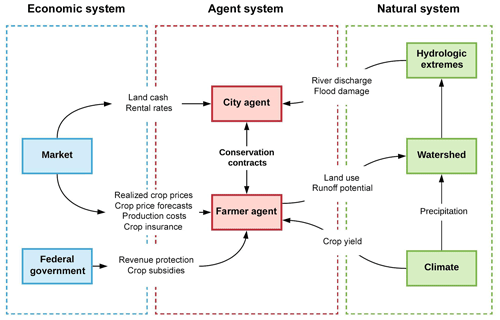
The model links an agent-based model of human decision-making with a rainfall–runoff model to simulate social and natural processes within highly managed agricultural watersheds (Fig. 1). The agent-based model consists of two types of agents: a group of farmer agents and a city agent.

The primary modeling domain consists of the watershed and the subbasins located within the watershed. The model user must define the subbasins based on external analyses of hydrologic flows and conditions. Each subbasin is populated by one or more farmer agent as specified by the user. A farmer agent modifies the land use of the subbasin in proportion to the subbasin area assigned to that agent. The most downstream subbasin in the watershed is populated by an urban center, which is represented by a city agent. The city agent impacts land use by providing subsidies to upstream farmer agents to change their land management.

2.1.1 Farmer agent state variables

The primary state variable for a farmer agent is the conservation parameter (Cons_max), which characterizes the degree to which a farmer agent is “production-minded” versus “conservation-minded”. This concept is based on McGuire et al. (2013) who identified that US Corn Belt farmers tend to fall along a spectrum from purely productivist to purely conservationist. Cons_max is randomly assigned to each farmer agent upon initialization and provides variation in farmer agent behavior based on how an individual agent may prefer to balance maximizing crop yields versus protecting the environment. Cons_max represents the maximum fraction of land a farmer is willing to put into conservation. The minimum value is 0.0, in which case a farmer is purely production-minded and is unwilling to convert any production land into conservation. We set the maximum value at 10 % (Cons_max=0.10) based on the conservation practice used in this study (Sect. 2.7.1). Therefore, a farmer is purely conservation-minded at a parameter value of 0.1, and is willing to convert up to 10 % of their production land into conservation. This range of values corresponds to the percentage of conservation land implemented over each of the last 10 years for the entire state of Iowa (∼5 %–6 % conservation land) and the central Iowa agricultural district (∼3 %–4 % conservation land).

A secondary state variable of importance to the farmer agent is risk aversion attitude (Prokopy et al., 2019). Risk aversion can be defined as the willingness to change land use under uncertainty. Farmers with a high risk aversion are unwilling to change their land use practices because they are trying to avoid risk. Keeping their land use consistent represents a more predictable payoff, even if the revenue may not be as great as another land use choice. However, farmers that are more risk tolerant are more likely to adopt new practices such as conservation. Farmer agents are further characterized by their decision-making preferences, which describe the relative importance that farmer agents place on different decision variables when adjusting their land use. The farmer agent decision characteristics are described in Sect. 2.7.2.

Each farmer agent is assigned state variables characterizing the percent of different soil types associated with the farmer's land. Corn crop productivity and crop production costs (including the land rental value) vary for each soil type. Thus, the soil types associated with a farmer agent's land impact their revenue.

Figure 2 Timeline of agent decisions and actions within the agent-based model.

2.1.2 City agent state variables

The city agent is characterized by a conservation goal that defines the amount of acres of conservation land desired. The purpose of the conservation land is to reduce flooding in the city, and the conservation goal changes from year to year depending on prior hydrologic events. The damage that the city agent incurs from a flood event is defined by a flood damage function. A parameter, ConsGoal_max, in the agent model defines how responsive the city agent is to prior hydrologic outcomes and determines how much the city agent will change the conservation goal by after experiencing a flood event (Sect. 2.8)

2.2 Model overview and scheduling

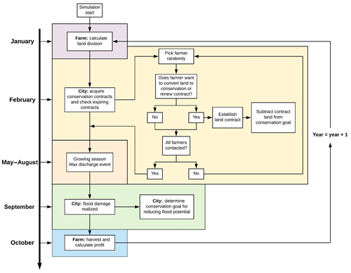
Each year, the agent-based model proceeds through monthly time steps to simulate the relevant decision-making. The hydrologic module proceeds in shorter hourly time steps to capture flood discharge events associated with rainfall events. Figure 2 depicts the decision-scheduling within the agent-based model. In January, the farmer agent calculates their preferred land division between production and conservation based on their risk aversion attitude, conservation-mindedness, newly acquired information about the global market (crop prices, crop production costs, and crop insurance), conservation subsidies provided by the city agent, and recent farm performance (profits and yields; Fig. 2, purple box).

In February, the city agent contacts farmer agents in random order to establish new conservation contracts if an unmet conservation goal remains or to renew any expiring contracts (Fig. 2, yellow box). If the farmer agent wants to add additional conservation acreage, a new contract is established for a 10-year period. The contract length is based on the Conservation Reserve Program (CRP), which is a program administered by the Farm Service Agency that promotes the removal of environmentally sensitive land from agricultural production in exchange for an annual subsidy payment. However, if the farmer agent wants fewer conservation hectares, expiring contracts are renewed for a smaller number of hectares or are ended. The farmer is obligated to fulfill any contracts that have not yet expired (i.e., contracts less than 10 years old). Any new acreage that has been established in conservation in addition to currently active contracts is subtracted from the city agent's conservation goal that was established in January. The city agent contacts as many farmer agents as needed until the conservation goal is reached. If there are not enough farmer agents willing to enter into conservation contracts and the conservation goal is not reached, the goal rolls into the next year. Because the farmer agents' land use decisions change on a yearly basis, it may be possible for the city agent to establish further contracts in the next year and fulfill the conservation goal.

Prior to May, the farmer agent establishes any newly contracted conservation land on the historically poorest yielding land. The farmer agent makes no further decisions during May through August (Fig. 2). The city agent continuously keeps track of any flooding that occurs during the May–August period (when the maximum discharge is assumed to occur; Fig. 2, orange box). The associated flood damage cost is calculated in September and used to calculate whether any further conservation land should be added (Fig. 2, green box). If no flooding occurred, the conservation goal remains unchanged. In October, the farmer agent harvests their crop and calculates yields and profits for that year (Fig. 2, blue box).

2.3 Design concepts

Emergence: patterns in total conservation land and flood magnitude arise over time, depending on a number of variables. Agent decision-making parameters and behavioral characteristics (e.g., conservation-mindedness) influence the total acreage in conservation land, which in turn affects the magnitude of floods through changes in runoff productivity of the landscape.

Objectives and Adaptation: the goal of the city agent is to reduce flood damage in the city. The city agent attempts to meet this goal through an incentive program in which farmer agents are paid to convert production land to a conservation practice that will reduce runoff. If the city agent incurs a large cost from flooding in a given year, the city agent adjusts their “conservation goal” upward in order to reduce future flood damage from events of similar magnitude. The objective of the farmer agent is to balance profits with conservation and risk aversion attitude. The farmer agents incrementally adjust their land use on an annual basis by taking profit variables, risk aversion, and conservation-mindedness into account.

Stochasticity: adjustments and stochastic variability are added to key agricultural variables, which include crop yields, production costs, cash rent values, and opportunity costs associated with conservation land in order to account for economic and environmental randomness within the system (Sects. S1.1, S1.2, and S2 in the Supplement). Random factors for these variables are drawn from uniform continuous distributions that are based on field data of crop yields, empirical survey data, and estimates published by Iowa State University Extension and Outreach. Changes in these distributions are also accounted for, depending on crop price levels.

Learning: as will be outlined further in Sect. 2.7.2, each year, the farmer agents calculate profit differences between crop production and conservation subsidies. Farmer agents save this profit difference information from the beginning of the simulation and use it to adjust their decision-making space on an annual basis. The profit difference information is based on past crop prices, production costs, and conservation subsidies.

2.4 Model input

2.4.1 Economic inputs

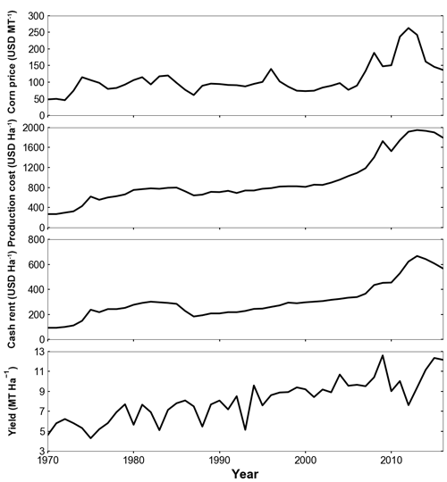
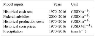
Inputs to the agent-based models are historical crop prices (USD MT⁻¹), production costs (USD ha⁻¹), cash rental rates (USD ha⁻¹), and federal government subsidy estimates (USD ha⁻¹). An example of these model inputs is shown in Fig. 3 in comparison to mean Iowa crop yields.

Figure 3 Example input time series of corn price, production cost, and cash rent compared with mean crop yields.

2.4.2 Production costs

Production costs are treated as a time series input, with total costs per hectare for each year represented by one lumped value. Production costs used in this model application include land rent, machinery, labor, crop seed, chemicals, and crop insurance (Plastina, 2017). As estimates put the amount of land rented out in Iowa for farming at 60 %–80 %, it is assumed that all farmer agents rent their land (Plastina et al., 2018; Zhang, 2015). This significantly increases expenses as land rental costs account for approximately half of total production costs (Plastina, 2017).

2.4.3 Conservation subsidy and costs

The conservation subsidy is based on the CRP “Contour Grass Strips” practice (CP-15A) which includes annual land rental payments and 90 % cost share for site preparation and establishment (USDA Conservation Reserve Program Practice CP-15A; USDA, 2015). Subsidies are calculated using annual inputs of historical cash rental rates. The cost of establishing and maintaining conservation land is based on analysis conducted by Tyndall et al. (2013). These costs are adjusted based on the land quality of each farmer agent (Sect. S1.2).

2.4.4 Federal government subsidies

Calculation of federal government crop subsidies for individual farmer agents were not included in the agent-based model due to the complexity and variety of commodity programs available to US farmers, each of which focuses on different aspects of revenue protection (e.g., protection against low crop prices and protection against revenue loss). Rather, federal crop subsidies are an input to the model and applied equally to each farmer agent. In this study, crop subsidy inputs are based on historical estimates produced by Iowa State University Agricultural Extension (Hofstrand, 2018).

2.4.5 Environmental variables

The hydrology module requires hourly liquid precipitation (mm) as an input to simulate discharge from short-term heavy rainfall events. The crop yield module requires inputs of mean monthly precipitation and temperature to estimate crop yields (Sect. 2.6). The module calculates mean monthly precipitation based on the hourly precipitation input; however, the user must provide an input of mean monthly temperatures (^∘C).

2.5 Hydrology module

A model structure that is designed to simulate peak flows was chosen for the hydrology module. Because the city agent in this model is impacted only by the maximum annual peak flow, precisely simulating the full time series of hydrologic flows as well as hydrologic components such as groundwater flow and evapotranspiration were not needed to meet the objectives of the current study. The modeling structure was designed based on a version of the US Army Corps of Engineers' Hydrologic Engineering Center Hydrologic Modeling System (HEC-HMS) (Scharffenberg, 2013) used by the City of Ames, Iowa, for flood forecasting in the Squaw Creek watershed in central Iowa. The Squaw Creek watershed represents the type of rural–urban conditions of interest for this study and is a useful test bed for this modeling application (Sect. 3). Further, calibrated parameters were available for the Squaw Creek watershed (Schmieg et al., 2011), providing a realistic baseline for the hydrology module.

Using the configuration and parameters previously defined by Schmieg et al. (2011) for the Squaw Creek watershed, the model was within 12.7 % on average of the observed peak discharge for 12 major events simulated. Six of these events were simulated within 3 %–8 % of the observation, while the least satisfactory simulation overestimated the observed peak discharge by 33 %. This error was most likely due to the high spatial variability of precipitation for that event. For the two most recent record flooding events, the model underestimated the peak discharge by 6.2 % (2008; observed: 356.7 m³ s⁻¹; simulated: 334.6 m³ s⁻¹) and 16.6 % (2010; observed: 634.3 m³ s⁻¹; simulated 528.3 m³ s⁻¹), showing that the model is able to simulate the flooding events needed to run scenarios within the ABM with a fair degree of accuracy. The HEC-HMS model has also been successfully used for simulation of short-term rainfall–runoff events and peak flow and flood analysis in other studies (Chu and Steinman, 2009; Cydzik and Hogue, 2009; Gyawali and Watkins, 2013; Halwatura and Najim, 2013; Knebl et al., 2005; Verma et al., 2010; Zhang et al., 2013).

In the module, basin runoff is computed using the Soil Conservation Service (SCS) curve number (CN) method, runoff is converted to basin outflow using the SCS unit hydrograph (SCS-UH) method, and channel flow is routed through reaches in the river network using the Muskingum method (Mays, 2011). A single area-weighted CN parameter is required for each subbasin and is the only hydrology module parameter that changes during the simulation if land cover changes. The SCS-UH method requires the specification of subbasin area, time lag, and model time step. The Muskingum method is based on the continuity equation and a discharge–storage relationship which characterizes the storage in a river reach through a combination of wedge and prism storage (Mays, 2011). The Muskingum method requires specification of three parameters for each reach within the river network: Muskingum X, Muskingum K, and the number of segments over which the method will be applied within the reach (Mays, 2011). Muskingum X describes the shape of the wedge storage within the reach, whereas Muskingum K can be approximated as the travel time through the reach.

For the agricultural areas, empirically derived CN values (Dziubanski et al., 2017) are used for native prairie strips; a CN of 82 is used for 100 % row crop production; and a CN of 72 is used for the conservation option implemented by the farmer agents. Urban areas are set to a CN of 90 which is derived from the standard lookup tables for residential areas with lot sizes of 0.051 ha or less (soil group C; USDA-NRCS, 2004). Subbasin delineations and Muskingum parameters previously defined by Schmieg et al. (2011) are used.

The model accepts point-scale rainfall data (e.g., rain gauge data) and calculates mean areal precipitation using the Thiessen polygon gauge weighting technique (Mays, 2011). The Thiessen weights are entered as parameters to the module. For the initial testing presented in this paper, uniform precipitation over the entire watershed was assumed.

Output from the hydrology module is discharge at the watershed outlet (m³ s⁻¹). The hydrology module is run continuously but is designed primarily for the simulation of peak flows, which generally occur during the summer in the study region; therefore, for simplicity, a constant baseflow is assumed and snow is ignored. Runoff, river routing processes, and discharge are computed at a time step identical to the input rainfall data. The model is run at an hourly time step in this study, but is capable of running at a 30 min time step.

2.6 Crop yield module

Crop yields are modeled with a multiple regression equation that takes monthly precipitation and temperature into account. The regression equation, which was developed using historical crop yield and meteorological data for Iowa from 1960 to 2006, can be represented as follows (Tannura et al., 2008):

$$\begin{array}{}\text{(1)}& {\displaystyle }\begin{array}{rl}{\mathrm{yield}}_t& ={\mathit{\beta }}_{\mathrm{0}}+{\mathit{\beta }}_{\mathrm{1}}\left({\mathrm{year}}_t\right)+{\mathit{\beta }}_{\mathrm{2}}\left(\mathrm{September}\mathrm{through}\mathrm{April}\mathrm{precipitation}\right)\\ & +{\mathit{\beta }}_{\mathrm{3}}\left(\mathrm{May}\mathrm{precipitation}\right)+{\mathit{\beta }}_{\mathrm{4}}\left(\mathrm{June}\mathrm{precipitation}\right)\\ & +{\mathit{\beta }}_{\mathrm{5}}(\mathrm{June}\mathrm{precipitation}{)}^{\mathrm{2}}+{\mathit{\beta }}_{\mathrm{6}}(\mathrm{July}\mathrm{precipitation})\\ & +{\mathit{\beta }}_{\mathrm{7}}(\mathrm{July}\mathrm{precipitation}{)}^{\mathrm{2}}+{\mathit{\beta }}_{\mathrm{8}}(\mathrm{August}\mathrm{precipitation})\\ & +{\mathit{\beta }}_{\mathrm{9}}(\mathrm{August}\mathrm{precipitation}{)}^{\mathrm{2}}+{\mathit{\beta }}_{\mathrm{10}}(\mathrm{May}\mathrm{temperature})\\ & +{\mathit{\beta }}_{\mathrm{11}}\left(\mathrm{June}\mathrm{temperature}\right)+{\mathit{\beta }}_{\mathrm{12}}\left(\mathrm{July}\mathrm{temperature}\right)\\ & +{\mathit{\beta }}_{\mathrm{13}}\left(\mathrm{August}\mathrm{temperature}\right)+{\mathit{\epsilon }}_t.\end{array}\end{array}$$

Mean error of the above regression for Iowa over the 1960–2016 period is −0.395 MT ha⁻¹, and mean absolute error is +0.542 MT ha⁻¹. An error correction factor of +0.395 MT ha⁻¹ was added to the yield for each year to correct for this error. The above regression model is only appropriate for reproducing mean historical crop yields. As each farmer's land can be composed of different soil types, adjustments are applied to the crop yield for each soil type to account for differences in soil productivity (Sect. S2).

2.7 Farmer agent module

2.7.1 Conservation option

The conservation option implemented by farmer agents is native prairie strips, a practice in which prairie vegetation is planted in multiple strips perpendicular to the primary flow direction upland of and/or at the farm plot outlet (Dziubanski et al., 2017; Helmers et al., 2012; Zhou et al., 2010). Either 10 % or 20 % of the total field size is converted into native prairie vegetation under this practice. Prairie strips have been shown to reduce runoff by an average of 37 % (Hernandez-Santana et al., 2013) and have the additional benefits of reducing nutrients (Zhou et al., 2014) and sediments (Helmers et al., 2012) in runoff. The greatest runoff reduction was realized under the 10 % native prairie cover; therefore, the most conservation-minded farmers (Cons_max=0.10) in the model potentially convert up to 10 % of their total land into native prairie.

2.7.2 Farmer agent land use decision process

Agents within an ABM can be modeled using a variety of decision models with varying degrees of complexity (An, 2012; Zenobia et al., 2009). The study by An (2012) compiled a list of nine of the most common decision models used in agent-based modeling studies. Examples of a few of these include microeconomic models, space-theory-based models, cognitive models, and heuristic models. In microeconomic models, agents are typically designed to determine optimal resource allocation or production plans such that profit is maximized and constraints are obeyed (Berger and Troost, 2014). Example studies using optimization include Becu et al. (2003), Ng et al. (2011), and Schreinemachers and Berger (2011). In heuristic-based models, agents are set up to use “rules” to determine their final decision (Pahl-wostl and Ebenhöh, 2004; Schreinemachers and Berger, 2006). The “rules” are typically implemented using conditional statements (e.g., if..., then...). Example studies using heuristics include Barreteau et al. (2004), Le et al. (2010), Matthews (2006), and van Oel et al. (2010).

We take a different approach from the aforementioned studies by modeling agent decision-making using a nudging concept that originated in the field of data assimilation (Asch et al., 2017). Agents nudge their decision based on outcomes (i.e., flood damage and farm profitability) from the previous year. Information relevant to an individual agent is mapped into the decision space through a weighting function that updates the previous year's land use decision to create a new decision for the current year. The approach used for both agents is different from optimization in that the agents are not trying to determine the best decision for each year. These types of agents behave based on the idea of “bounded rationality”. In this case, the rationality of the agents is limited by the complexity of the decision problem and their cognitive ability to process information about their environment (Simon, 1957). These agents try to find a satisfactory solution for the current year, and they are thus termed “satisficers” rather than optimizers (Kulik and Baker, 2008).

Table 1 Variables in farmer and city agent equations.

Table 2 Primary agent model parameters in decision-making equations.

At the start of each calendar year, a farmer agent decides how to allocate their land between production and conservation based on five variables: risk aversion, crop price projections, past profits, conservation goal, and neighbor land decisions. These factors were chosen based on numerous studies indicating profits, economic incentives, conservation beliefs, beliefs in traditional practices, neighbor connections, and observable benefits to be the key factors influencing on-farm decision-making related to conservation adoption (Arbuckle, 2017; Arbuckle et al., 2013; Burton, 2014; Daloǧlu et al., 2014; Davis and Gillespie, 2007; Hoag et al., 2012; Lambert et al., 2007; McGuire et al., 2015; Nowak, 1992; Pfrimmer et al., 2017; Prokopy et al., 2019; Ryan et al., 2003).

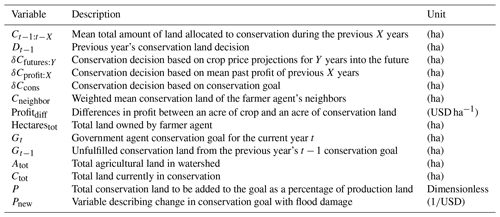
A farmer agent's decision of the total amount of land to be allocated into conservation, D_t, for the current year t is

$$\begin{array}{}\text{(2)}& \begin{array}{rl}{D}_t& =W_{\mathrm{risk}\text{-}\mathrm{averse}}\left[C_{t-\mathrm{1}:t-X}\right]+W_{\mathrm{futures}}\left[D_{t-\mathrm{1}}+\mathit{\delta }{C}_{\mathrm{futures}:Y}\right]\\ & +W_{\mathrm{profit}}\left[D_{t-\mathrm{1}}+\mathit{\delta }{C}_{\mathrm{profit}:X}\right]+W_{\mathrm{cons}}\left[D_{t-\mathrm{1}}+\mathit{\delta }{C}_{\mathrm{cons}}\right]\\ & +W_{\mathrm{neighbor}}\left[C_{\mathrm{neighbor}}\right],\end{array}\end{array}$$

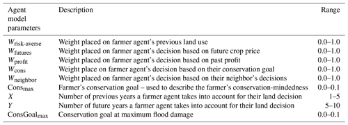
where $C_{t-\mathrm{1}:t-X}$ is the mean total amount of land allocated to conservation during the previous X years, D_t−1 is the prior conservation decision (total amount of land the farmer would have liked to implement in conservation) in year t−1, δC_futures:Y is the decision based on crop price projections for Y years into the future, δC_profit:X is the decision based on the mean past profit of the previous X years, δC_cons is the decision based on the conservation goal of the farmer, and C_neighbor (Sect. S3) is the weighted mean conservation land of the farmer agent's neighbors (Table 1). A given farmer can make a certain random number of neighboring connections with farmers that are located in the same subbasin (Sect. S3). The variable Y indicates that one farmer agent might consider their history of conservation land implemented over the last year, while another farmer agent might consider their conservation land implemented over the last 5 years. Similarly, the variable X indicates that one farmer agent might take future crop projections for the next 5 years into account, while another farmer agent might consider crop projections for the next 10 years.

Decision weights alter how each of the five components factor into the farmer agent's decision: W_risk-averse reflects the unwillingness to change past land use, W_futures reflects the consideration of future price projections, W_prof reflects the consideration of past profits, W_cons is the agent's consideration of their conservation goal, and W_neighbor reflects the importance that the agent places on their neighbor's decision (Table 2). Upon initializing each farmer agent, values are allocated for each decision weight such that

$$\begin{array}{}\text{(3)}& W_{\mathrm{risk}\text{-}\mathrm{averse}}+W_{\mathrm{futures}}+W_{\mathrm{profit}}+W_{\mathrm{cons}}+W_{\mathrm{neighbor}}=\mathrm{1}.\end{array}$$

The above decision scheme allows for varying decision weights; thus, one farmer's decision may be heavily weighted by future crop prices, whereas another farmer's decision may be heavily weighted by past profits. If the majority of a farmer's decision is based on W_risk-averse, then that farmer is less inclined to change their previous land use.

The decision components for past profit and future crop prices are based on a partial budgeting approach that compares land use alternatives. Under this budgeting approach, farmer agents take added and reduced income into account, as well as added and reduced costs from changing an acre of land from crop production to conservation (Tigner, 2006). The result from performing this budget indicates the net gain or loss in income that a farmer agent may incur if they make the land conversion.

The past profits decision is solely based on outcomes that have been fully realized for the previous X years. In this decision, the land allocated to conservation is based on the net amount of money that could have been earned per hectare of conservation land versus crop land and is calculated as follows:

$$\begin{array}{}\text{(4)}& \begin{array}{rl}\mathit{\delta }{C}_{\mathrm{profit}:X}& =\left[A\cdot {\mathrm{Profit}}_{\mathrm{diff}}^{\mathrm{2}}+B\cdot {\mathrm{Profit}}_{\mathrm{diff}}+C\right]\cdot {\mathrm{Cons}}_{\max }\\ & \cdot {\mathrm{Hectares}}_{\mathrm{tot}},\end{array}\end{array}$$

where Profit_diff is the difference in profit between a hectare of cropland and a hectare of conservation land (Table 1), Cons_max is the farmer agent's maximum conservation parameter, and Hectares_tot is the area of the agent's land. Profit_diff integrates costs and revenue of crop production as well as costs and revenue of conservation land, which are computed based on model input data (Sects. 2.4 and S4). In the case of δC_profit:X, Profit_diff is calculated using realized crop prices from previous years (Sect. S4). The future price decision variable, δC_futures:Y, is also calculated using the same form of Eq. (4). However, Profit_diff is calculated using projected crop prices for the Y upcoming growing seasons. These price projections are based on historical crop prices with an added adjustment calculated from historical errors in crop price forecasts produced by the US Department of Agriculture (Sect. S5).

The first term in Eq. (4), the second-degree polynomial of form $A{x}^{\mathrm{2}}+Bx+C=y$, is displayed in Fig. 4. At the start of each year, farmers may decide to alter their land use based on observed Profit_diff from harvests in previous years (δC_profit:X) or calculated Profit_diff based on projected crop prices (δC_futures:Y). If Profit_diff is positive (i.e., greater profit is earned from crop production than conservation land), the farmer agent will potentially decrease the amount of land in conservation (gray curve). Likewise, under negative Profit_diff, conservation land is potentially increased because revenue is lower from crop production (black curve). Half of the maximum allowable percent increase in conservation land is assumed to correspond to the median historical negative Profit_diff, whereas half of the maximum allowable percent decrease in conservation land corresponds to the median historical positive Profit_diff (Fig. 4). We assume that farmer agents will not change land use when a very small profit difference between the two possible options is observed because changing land use requires extra upfront time and resources (Duffy, 2015). Similarly, we assume that farmer agents will fully implement the maximum land conversion possible prior to reaching the most extreme Profit_diff values. Three equations need to be simultaneously solved to determine coefficients A, B, and C (Sect. S4). The three equations are based on the median and the 25th and 75th percentiles of historical Profit_diff information. Thus, farmers are continually utilizing historical observations of Profit_diff to formulate their decision space through time.

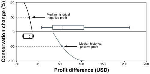
Figure 4 Example of percent conservation change for δC_profit and δC_futures. Gray curves indicate negative percent change (decrease in conservation land), and black curves indicate positive percent change (increase in conservation land).

The use of a profit function (i.e., Eq. 4) is meant to capture the effects of changes in crop prices on conservation land. In 2008 and 2011, corn prices rose to a record high values, and farmers in the Midwest US (e.g., Iowa and Minnesota) were converting significant portions of CRP land back into crop production (Marcotty, 2011; Secchi and Babcock, 2007). It is estimated that when corn prices rise by USD 1.00, 10 %–15 % of CRP land in Iowa is converted back to production (Secchi and Babcock, 2007). Equation (4) captures this transition between adding and removing conservation land based on crop price change, and it allows for variation in the decision-making between farmer agents as variables such as crop production costs vary from farm to farm.

The total amount of agricultural land that a farmer converts to conservation in any given year based on their conservation goal (δC_cons) is defined by the Bernoulli distribution:

$$\begin{array}{}\text{(5)}& P\left(n\right)=p^n(\mathrm{1}-p{)}^{\mathrm{1}-n}n\in \mathit{\{}\mathrm{0},\mathrm{1}\mathit{\}}.\end{array}$$

Here, p indicates the probability of fully implementing conservation land, and 1−p indicates the probability of not implementing any conservation land. The variable n is simply the support of the distribution that labels a success of full implementation as 1 and a failure of full implementation as 0. The probability p of fully implementing conservation land is a function of the agent's Cons_max parameter and is computed by

$$\begin{array}{}\text{(6)}& p=\mathrm{10}\cdot {\mathrm{Cons}}_{\max }.\end{array}$$

The probability p scales from 0 at a Cons_max of 0, to 1 at a Cons_max of 0.1. Therefore, farmer agents with a Cons_max of 0.05 and 0.1 will have a 50 % and 100 % probability of fully implementing (10 % of total agricultural land) conservation land in any given year based on their conservation decision variable.

2.8 City agent module

At the end of each year, the city agent collects discharge data and calculates the damage (Sect. S7) associated with the peak annual discharge at the watershed outlet for that year. In February of the next year, the flood damage for the previous year t−1 is used to compute the conservation goal of the city agent for the current year t.

The conservation goal of the city agent is calculated as follows:

$$\begin{array}{}\text{(7)}& {\displaystyle }& {\displaystyle }{G}_t=G_{t-\mathrm{1}}+\left(A_{\mathrm{tot}}-C_{\mathrm{tot}}\right)\cdot P\text{(8)}& {\displaystyle }& {\displaystyle }P=P_{\mathrm{new}}\cdot \mathrm{FDam}\text{(9)}& {\displaystyle }& {\displaystyle }{P}_{\mathrm{new}}={\displaystyle \frac{{\mathrm{ConsGoal}}_{\max }}{\mathrm{FDmax}}},\end{array}$$

where G_t is the conservation goal for the new year t (Table 1), G_t−1 is the unfulfilled hectares in conservation from the previous conservation goal for year t−1, A_tot is the total land area owned by the farmer agents, C_tot is the total number of hectares currently in conservation, P is the percentage of new production land added into conservation, P_new indicates how much land to add into conservation based on the flood damage FDam for year t−1, and ConsGoal_max is a parameter that indicates the new percentage of conservation land to be added if maximum flood damage occurs (Table 2). Currently, ConsGoal_max is set to 5 % of total land area in the watershed when maximum damage occurs.

3 Scenario analysis

The study watershed is modeled after the Squaw Creek basin (∼56 200 ha) located in central Iowa, USA (Fig. 5). This basin is characterized by relatively flat hummocky topography and poorly drained soils with a high silt and clay content (∼30 %–40 % silt and clay) (Prior, 1991; USDA-NRCS, 2015). The predominant land use is row crop agriculture (∼70 % of the total watershed area) with one major urban center at the outlet (Ames, Iowa) and several small communities upstream. Average annual precipitation is 32 inches (812 mm), with the heaviest precipitation falling during the months of May and June. The watershed is divided into 14 subbasins.

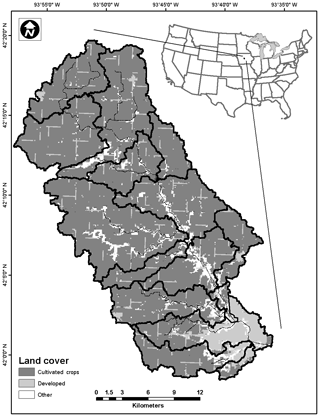
Figure 5 Squaw Creek watershed and subbasin division used in the hydrology module. Land cover data shown are from the National Land Cover Database (Dewitz, 2019).

In this model application, 100 farmer agents are implemented (∼7 farmers per subbasin) with 121 ha total for each farmer. The total acreage per farmer compares reasonably well with the average farm size for the state of Iowa in 2017, which was 140 ha (USDA, 2018). Soil types and the area of land associated with each soil type are randomly assigned to each farmer agent upon model initialization. Assigning different soil types creates heterogeneous conditions under which farmer agents must operate (Sect. S2) and affects the profitability of each farmer agent differently.

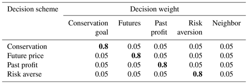
Six scenarios are run: high and low yield (±11 % from historical yield), high and low corn prices (±19 % from historical prices), and high and low conservation subsidies (±27 % from historical cash rent). The watershed was also simulated under historical conditions, in which no economic variables were changed, for comparison purposes. The 90th percentile discharge is analyzed, which represents the 0.1 exceedance probability level, to examine changes in large discharge events. The above percentages were computed using trends and mean absolute deviations of historical economic data. For instance, based on the crop regression model (Sect. 2.6), crop yields display a relatively linear increase with time. The mean absolute deviation of the crop yield was then computed using the linear time trend as a central tendency. The mean absolute deviation was determined to be 11 %; thus, the yield scenarios are ±11 % from the historical yield. The same approach was used for the crop price and conservation subsidy scenarios. A linear and cubic function were found to provide a good estimate of the central tendency of historical cash rent and crop prices, respectively, for those calculations. In addition, four different farmer decision schemes were created in which an 80 % weight was assigned to one decision variable, with all other variable weights set to 5 % (Table 3). Each scenario is tested with each decision scheme, and system outcomes under different farmer behaviors are assessed.

Table 3 Decision weighting scheme tested with each scenario. Bold numbers indicate the decision variable assigned 80 % weight for each decision scheme.

To test the sensitivity of the hydrologic system to farmer types, the conservation parameter (Cons_max) of the farmer agents is varied using a stratified sampling approach. Each farmer agent is randomly assigned a Cons_max value from a predefined normal distribution: ($\stackrel{\mathrm{‾}}{{\mathrm{Cons}}_{\max }}$, ${\mathit{\sigma }}_{{\mathrm{Cons}}_{\max }}$). The lowest distribution is defined as N(0.01, 0.01) and the highest distribution is defined as N(0.09, 0.01). Any farmer agent that is assigned a parameter value less than 0 or greater than 0.1 is modified to have a value of 0 or 0.1, respectively. A total of 12 simulations are performed for each conservation parameter distribution, with a total of 17 conservation parameter distributions. Thus, the first 12 simulations consist of farmer agents with Cons_max chosen from N(0.01, 0.01). For the next 12 simulations, the mean Cons_max is shifted up by 0.05, with Cons_max chosen from N(0.015, 0.01). A total of 204 simulations are conducted for each decision scheme under each scenario (Table 3).

Each simulation is run using 47 years of historical climate and market data, with the exception of federal crop subsidies, which are based on 16 years of historical estimates produced by Iowa State University Agricultural Extension (Hofstrand, 2018; Table 4). It is assumed that federal crop subsidy payments from 1970 to 2000 are similar to levels seen from 2000 to 2005 due to relative stability of long-term crop prices and production costs. The hourly 47-year precipitation time series data were obtained from the Des Moines, Iowa airport Automated Surface Observing System. Historical 47-year time series of corn prices, crop production costs, and land rental values are used as economic inputs into the model and were obtained from Iowa State University Agricultural Extension and Illinois farmdoc (Table 4).

Table 4 Model inputs.

4 Model calibration and validation

Calibrating and validating the social part of social–hydrologic models is difficult due to the lack of sufficiently detailed empirical data or system complexity at various scales, among other reasons (An, 2012; Ormerod and Rosewell, 2009; Troy et al., 2015). Validation of agent-based models is usually performed on what term the micro and macro levels. The micro level involves comparing individual agent behaviors to real-world empirical data, whereas the macro level involves comparing the model's aggregate response to system-wide empirical data (An et al., 2005; Berger, 2001; Troy et al., 2015; Xiang et al., 2005). Troy et al. (2015) suggests that one or a few model simulations out of an ensemble of simulations should match the real-world observed data.

We conduct an indirect macro-level model calibration for determining an appropriate range of farmer agent decision weights (Windrum et al., 2007). As the subsidy program offered by the city agent is similar to the federal Conservation Reserve Program (CRP), the model was developed and calibrated to attempt to reproduce the range and variability of conservation land seen in the CRP program. CRP data from 1986 to 2016 for the central Iowa agricultural district were used in the calibration process, and two main objectives functions were used:

$$\begin{array}{}\text{(10)}& \mathrm{MAE}={\displaystyle \frac{\sum _{i=\mathrm{1}}^n\left|y_i-x_i\right|}{n}}\end{array}$$

$$\begin{array}{}\text{(11)}& \mathrm{Pearson}\text{'}\mathrm{s}r={\displaystyle \frac{\sum _{i=\mathrm{1}}^n\left(x_i-\stackrel{\mathrm{‾}}{x}\right)\left(y_i-\stackrel{\mathrm{‾}}{y}\right)}{\sqrt{\sum _{i=\mathrm{1}}^n{\left(x_i-\stackrel{\mathrm{‾}}{x}\right)}^{\mathrm{2}}}\sqrt{\sum _{i=\mathrm{1}}^n{\left(y_i-\stackrel{\mathrm{‾}}{y}\right)}^{\mathrm{2}}}}}.\end{array}$$

In the first step of calibration, the focus was to determine an appropriate range of mean ConsMax of the farmer agent population to match the magnitude of CRP land seen for central Iowa. The model was simulated 360 times using 20 random sets of farmer agent decision weights. Output from the first calibration step was filtered using a criteria of r>0.6 and MAE < 25 %, and the optimal ConsMax range was reduced to 0.05–0.07. In the second step of calibration, the focus was to determine a singular optimal mean ConsMax value and to narrow the range for each decision weight. ConsMax was incremented by 0.001 within the range derived from step 1, and 20 simulations were performed for each increment using decision weights stochastically drawn from the uniform distribution U(0.05, 0.95) for a total of 400 simulations. Output was filtered using a stricter criteria of r>0.7 and MAE < 25 %. The final calibration step involved 400 simulations with the optimal mean ConsMax value and stochastic sampling from the reduced range of decision weights derived in step 2. Filtering with a criteria of r>0.75 and MAE < 12.5 % was performed to determine the final optimal decision weight ranges.

The optimal mean ConsMax value was determined to be 0.06, and the final optimal decision weight ranges were determined to be W_risk-averse=(0.1, 0.43), W_futures=(0.07, 0.24), W_profit=(0.07, 0.34), W_cons=(0.18, 0.37), and W_neighbor=(0.05, 0.35). The median r and MAE values of the simulations after filtering with the criteria in step 3 (r>0.75, MAE < 12.5 %) were 0.79 % and 11 %, respectively. A total of 66 of the 400 simulations matched this criteria in step 3, whereas only 7 matched this criteria in step 1 and 26 matched this criteria in step 2.

The model-simulated conservation land generally aligns with trends in the observed conservation land (Fig. 6). Simulated conservation land is not maintained following a rise in crop prices in the mid-1990s and from 2006 to 2013, which is similar to the observed data (red). The drop in conservation land during these time periods occurs because the subsidy rate is not modified rapidly enough in comparison to market forces to incentivize the farmer (Newton, 2017). The model does capture the smaller decrease in conservation land between 2007 and 2014, even though crop prices rose more dramatically than in the mid-1990s.

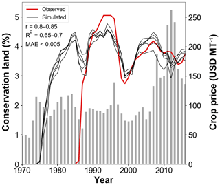
Figure 6 Simulated conservation land from four model simulations with Pearson's r>0.8 and MAE < 12.5 % compared with observed conservation land.

The onset of significant land conversion in the model is offset from the observations. Conservation land is implemented in the mid-1970s, while conservation land in the observation is implemented in the late 1980s. The CRP program did not come into existence until 1985, which partly explains this difference. A large rise in conservation land to roughly 4 % occurs from 1975 to 1978, most likely due to a combination of decreasing crop prices from 1974 to 1977 and model spin-up. This is similar to the rate of rise in conservation land that occurred under the CRP programs from 1985 to 1987 under a comparable period of decreasing crop prices.

Overall, calibration does provide evidence that the model captures changes in CRP land during the appropriate time periods. However, the calibration technique does have limitations. The technique followed here was an indirect calibration approach, whereby the parameters are determined based on the simulations that replicate the empirical data best (Fagiolo et al., 2006). This technique can lead to equifinality as different parameter sets may reproduce the historical observations with similar degrees of accuracy. Further, this calibration approach does not provide evidence that any individual agent's decisions are valid. The stochastic nature of human behavior coupled with path dependencies makes it difficult to predict individual agent outcomes accurately (Berglund, 2015). A dominating problem with calibrating ABMs is that it may be difficult to find sufficient data sets to support a robust validation at the micro level. For modeling land use decisions, data are typically available at a larger scale, such as county or state level, rather than at the individual agent level, such as a single farm (An, 2012; Parker et al., 2008). This introduces difficulty in trying to validate farm-level decisions with respect to farm-level finances (Sect. 2.7.2). Adding in additional factors, such as Federal Market Loss Assistance and Loan Deficiency Payments, as well as trying to characterize some of the other model parameters that were not a focus of this calibration, may further improve results.

In light of the paper by Windrum et al. (2007), there has been much debate as to the proper methodology and techniques to follow for ABM validation (Bharathy and Silverman, 2013; Hahn, 2013). To fully validate the current model, a more extensive process may be necessary. Macal and North (2005) introduced a framework for ABM validation that may provide for a more comprehensive evaluation. This framework includes subject matter expert evaluation, participatory simulation, model-to-model comparison, comparison against critical test cases, invalidation tests, and comprehensive testing of the entire agent strategy and parameter space. However, following this framework is very time intensive; thus, most recent studies have focused on empirical validation against real-world macro-level data, with some studies validating at the individual agent level if data are available (Fagiolo et al., 2019; Guerini and Moneta, 2017; Langevin et al., 2015; Schwarz and Ernst, 2009).

5 Results

5.1 Crop price scenarios

The 90th percentile peak discharge is 296.4 m³ s⁻¹ when no conservation is occurring in the watershed (Fig. 7). The 90th percentile peak discharge decreases for all four decision schemes and under all scenarios as the average conservation-mindedness (Cons_max) of the population increases (Fig. 7). The low crop price scenario produces a larger decline in peak discharge compared with the high crop price scenario, with the exception of the conservation decision scheme (80 % weight on conservation) in which both low and high crop price scenarios produce a similar ensemble pattern (Fig. 7a).

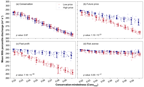
Figure 7 Mean 90th percentile discharge for high and low crop price scenarios with (a) 80 % weight on conservation goal, (b) 80 % weight on future price, (c) 80 % weight on past profit, and (d) 80 % weight on risk aversion. The circles indicate the median values and the bars show the 5th and 95th percentiles of discharge for all simulations at a specific Cons_max.

Under low crop prices, peak discharge reaches an average reduction of 8.18 % (24.27 m³ s⁻¹) when the average Cons_max is 0.08–0.09 (conservation-minded population) and 4.67 % (13.85 m³ s⁻¹) when the average Cons_max is 0.04–0.06 (mixed population). The decrease in peak discharge corresponds to the 800–1000 and 400–600 ha converted to conservation by the conservation-minded and mixed farmer populations, respectively (Fig. 8a, c, e, g). The production-minded populations (Cons_max∼0.01–0.02) implement less than 200 ha during the entire simulation period. These acreage values represent 6.5 %–8.2 %, 3.3 %–5.0 %, and less than 2.0 % of the entire watershed for the conservation-minded, mixed, and production-minded groups, respectively. Given that 10 % of the watershed would be under conservation if native prairie strips were fully implemented, about 65 %–80 % of a conservation-minded population fully implements the practice over the simulation period under low crop prices.

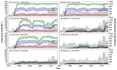
Figure 8 Range of simulated conservation land within the watershed with low (a, c, e, g) and high (b, d, f, h) crop prices for conservation-minded populations (green), mixed populations (blue), and production-minded populations (red). Crop prices are plotted as bars for each crop price scenario. Results are for decision schemes of 80 % weight on conservation behavior (a, b), 80 % weight on future price (c, d), 80 % weight on past profit (e, f), and 80 % weight on risk aversion (g, h).

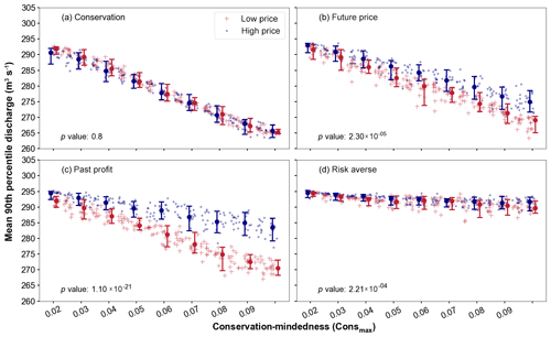
Figure 9 Mean 90th percentile discharge for high and low crop yield scenarios with (a) 80 % weight on conservation goal, (b) 80 % weight on future price, (c) 80 % weight on past profit, and (d) 80 % weight on risk aversion. The circles indicate the median values and the bars show the 5th and 95th percentiles of discharge for all simulations at a specific Cons_max.

Under the high crop prices, mean peak discharge decreases by 5.6 % (16.6 m³ s⁻¹) under the future price weighting scheme and 2.9 % (8.6 m³ s⁻¹) under the past profit weighting schemes for the highly conservation-minded population (Fig. 7b and c, respectively), with an even smaller reduction seen for the risk averse scenario. This represents approximately a 61 % smaller decrease in the peak discharge when crop prices are high and the population is conservation-minded compared with the low crop price scenario. Discharge remains largely unchanged for these decision schemes because generally less than 300 ha of land is allocated for conservation when corn prices are high (Fig. 8d, f, h). The small amount of conservation land implemented is due to farmer agents receiving significantly more revenue from crops than conservation subsidies. However, in the case of low crop prices, conservation subsidies allow the farmer agents to approach breakeven because they are guaranteed a subsidy that covers the cash rent for that land, whereas crop production leads to potential losses due to corn prices being low relative to production costs. Even in these scenarios where farmer agents are heavily considering profit-related variables, populations dominated by production-minded farmer agents are still inclined to leave land in production (Fig. 8c, e).

5.2 Crop yield scenarios

Under high and low crop yield scenarios, the 90th percentile peak discharge decreases by an average of 5.9 % (17.4 m³ s⁻¹) and 7.6 % (22.7 m³ s⁻¹), respectively, for the conservation-minded populations (Fig. 9). Thus, a smaller decrease in peak discharge occurs with low crop yields relative to low crop prices (Fig. 7). In the low crop yield scenario, conservation land was approximately 200 ha less than in the low crop price scenario, particularly for the past profit and future price decision schemes (Figs. 8a, c, e, g and 10a, c, e, g). Conversely, more conservation land is established under the high yield scenario compared with the high crop price scenario (Figs. 8b, d, f, h and 10b, d, f, h). As a result, mean peak discharge decreases in the high yield scenario by 15.6 % more than in the high crop price scenario for the conservation-minded population.

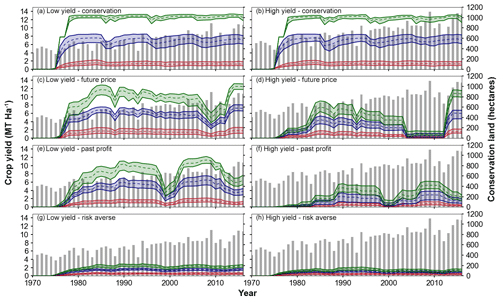
Figure 10 Range of simulated conservation land within the watershed with low (a, c, e, g) and high (b, d, f, h) crop yields for conservation-minded populations (green), mixed populations (blue), and production-minded populations (red). Yearly crop yields are plotted as bars for the crop yield scenario. Results are for decision schemes of 80 % weight on conservation behavior (a, b), 80 % weight on future price (c, d), 80 % weight on past profit (e, f), and 80 % weight on risk aversion (g, h).

5.3 Conservation subsidy scenarios

Under the low and high subsidies scenarios (not shown), the 90th percentile peak discharge decreases by an average of 5.8 % (17.3 m³ s⁻¹) and 7.6 % (22.5 m³ s⁻¹), respectively, for conservation-minded populations. Similar to the low crop yield scenario, high subsidies do not produce as much of a decrease in the mean peak discharge as low crop prices (Fig. 7). In the high subsidies scenario, conservation land was approximately 200–300 ha less than in the low crop price scenario, specifically for the future price and past profit decision scheme. In comparison, low subsides generate more conservation land than high crop prices (Fig. 8b, d, f and h). As a result, mean peak discharge decreases in the low subsidy scenario by 14.8 % more than in the high crop price scenario for the conservation-minded population. Differences in peak discharge reduction between the high subsidy and low yield scenarios were insignificant, with less than a 1 % difference between these two scenarios.

5.4 Decision schemes

The future price and past profit decision schemes display the largest spread in discharge outcomes between scenarios (Figs. 7, 9). Mean peak discharge decreases by 9 % (∼27.2 m³ s⁻¹) on average relative to when no conservation occurs for both decision schemes under all scenarios that encourage more conservation land, i.e., low crop prices, low yields, and high subsidies (Figs. 7b, c and 9b, c). Under scenarios that encourage less conservation land, mean peak discharge decreases by 5 % (∼15.4 m³ s⁻¹). This spread in the peak discharge results is not present in the risk averse and conservation decision schemes.

The spread between the mean peak discharge under the different scenarios is smaller for the future price decision scheme (Figs. 7b, 9b) compared with the past profit decision schemes (Figs. 7c, 9c). This smaller spread may be due to uncertainty in future crop price projections. For instance, future crop price projections may underestimate high crop prices, but overestimate low crop prices, as is observed in previous USDA crop price forecasts (Sect. S5). Thus, the farmer agents may be making decisions based on a smaller range of crop prices when under the future price decisions compared with the past profit decision scheme where they use realized crop prices. In addition, the future crop price decision scheme results in greater variability in conservation land over short periods of time under all scenarios (Figs. 8c, d and 10c, d). This result is evident under the low crop price scenario, with several short periods showing changes in conservation land of 200–400 ha compared with the past profit scenario where conservation land remains relatively steady. However, this result does not lead to a larger spread (i.e., red and blue bars) within the mean peak discharge results.

The risk averse decision scheme produces the smallest changes in peak discharge under all scenarios, with an average decrease of less than 2 % (6 m³ s⁻¹) and 3 % (9 m³ s⁻¹) for mixed and conservation-minded populations, respectively (Figs. 7d, 9d). Because the farmer's past practices are the primary factor in determining land conversion in this scheme, the farmer agents implement a limited number of conservation acres (≤200 ha), regardless of the scenario. Therefore, changes in the economic variables do not have as much of an impact on the farmer agents when they are strongly risk averse.

Overall, the current city agent conservation goal of 5 % new conservation land at maximum flood damage did not have a significant impact on the total amount of land implemented. Following two major flooding events, the conservation goal of the city agent increases from less than 20 ha in 1975 to 620 ha in 1976. A similar event in 1977 increases the conservation goal by another 500 ha for a total goal of approximately 1100 ha. These increases correspond to the large and rapid onset of conservation land seen during those years (Figs. 8a, c, e and 10a, c, e). After the 1977 flood event, several smaller flood events do occur that are generally less than 15 %–30 % of maximum, which further increases the conservation goal by ∼200–300 ha. When the population has a high average Cons_max, the conservation goal of the city agent is nearly fulfilled during this period, particularly in the low crop price scenario. In these cases, 900 ha of the conservation goal is implemented, and 200 ha remains unimplemented. This results in the largest reduction in 90th percentile discharge under all scenarios and decision schemes (Figs. 7a, 9a). When the population has a low average Cons_max, the majority of the city agent's conservation goal remains unimplemented. Thus, the goal remains at a constant 1000–1400 ha and discharge remains unchanged. The only case where the city agent conservation goal limits the amount of land implemented is under the conservation weighting scenario as conservation-minded farmers are inclined to add conservation land on a yearly basis.

5.5 Historical comparison

To gain an understanding of how each of the scenarios differs from the historical 1970–2016 period, the mean peak discharge is compared against the historical scenario (Fig. 11). Recall that under the historical scenario, farmer agents make annual land use decisions as in the other scenarios, but corn prices, conservation subsidies, and crop prices are unchanged from historical observed values. Overall, crop prices had the largest impact on mean peak discharge, while changes in subsidies had the smallest overall impact. When crop prices were low, mean peak discharge decreased by 1 %–2 % for mixed populations and 2 %–3 % for conservation-minded populations under the future price and past profit schemes compared with the historical scenario (Fig. 11a). High crop prices result in an increase in peak discharge from the historical scenario, with an increase of 1 %–3 % for mixed populations and 3 %–5 % for conservation-minded populations. This indicates that the farmer agents are more likely to convert land back to crop production under high crop prices than convert land to conservation under low crop prices, which is a similar conclusion to Claassen and Tegene (1999).

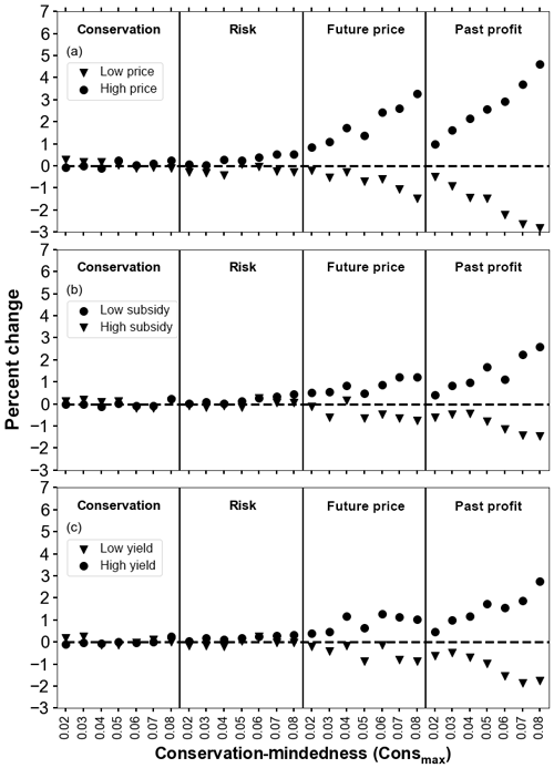
Figure 11 Percent change in median 90th percentile discharge from the historical scenario for (a) high and low crop prices, (b) high and low subsidies, and (c) high and low yields for the conservation, risk, future price, and past profit weighting schemes.

The subsidy scenarios produced a similar pattern to the crop price scenarios, where a larger change (increase) in mean peak discharge occurs under low subsidies than under high subsidies (Fig. 11b). This pattern was not as clearly evident under the yield scenarios, with similar changes resulting from high and low yields (Fig. 11c).

6 Conclusions

Scenarios of historical and low crop yields, as well as high and low corn prices and conservation subsidies, were simulated for an agricultural watershed in the Midwest US Corn Belt using an agent-based model of farmer decision-making and a simple rainfall–runoff model. The influence of different farmer agent decision components on model outcomes was also explored. Model results demonstrate causations and correlations between human systems and hydrologic outcomes, uncertainties, and sensitivities (specifically focused on high flows).

The primary findings of this study are as follows:

• Crop prices had the largest impact on mean peak discharge, with a 61 % larger reduction in mean peak discharge under low crop prices compared with high crop prices.

• Changes in subsidy rates and crop yields produced a smaller impact on mean peak discharge. Only a 25 %–30 % difference in mean peak discharge was realized between high and low subsidies, and high and low yields.

• Farmer agents more often made decisions to eliminate conservation land than to enter into conservation contracts: a 3 %–5 % increase in mean peak discharge occurred under high crop prices, while only a 2 %–3 % decrease in mean peak discharge occurred under low crop prices compared with the historical simulation. Thus, even under low crop prices, the effectiveness of the conservation program is limited either due to economic or behavioral factors.

• Hydrologic outcomes were most sensitive when farmer agents placed more weight on their future price or past profit decision variables and least sensitive when farmer agents were highly risk averse. For instance, under future price and past profit weighting scenarios, a 4 % and 7 % difference in mean peak discharge is seen between high and low crop prices as opposed to a 0 %–1 % difference under the risk averse weighting scenario.

The ABM modeling approach demonstrated here can be used to advance the fundamental understanding of the interactions of water resources systems and human societies, particularly focusing on human adaptation under future climate change. Our model indicates that external factors can influence local streamflow, albeit in a complex and unpredictable way as the information gets filtered through the complex decision-making of local farmers. Social factors, both local and external, introduce significant uncertainty in local hydrology outcomes, and by ignoring them, water management plans will be inherently incomplete. Thus, multi-scale human factors need to be explicitly considered when assessing the sustainability of long-term management plans.

This study additionally demonstrates some of the advantages of the ABM approach. One of the primary advantages of ABMs is the ability to capture emergent phenomenon (Bonabeau, 2002). For instance, in the model, the change in conservation area seen in the mid-1990s is larger than during the period after 2007, despite the much larger volatility in crop prices after 2007. While the primary reason behind this phenomenon may not be clear, the ABM captures this change. The ABM also allows for the specification of small-scale differences between farmer agents such as variations in conservation-mindedness, production costs, yields, and cash rents. Thus, using ABMs allows for a very flexible modeling approach.

The current model design contains limitations in both the hydrologic and agent-based models that should be addressed in future model development. The curve number values that were used to represent the conservation option were derived for small agricultural plots of approximately 0.5–3 ha in size. The question remains regarding whether these CN values can be scaled up to the size of a several hundred hectare farm plot and still produce reasonable discharge results. In addition, there is no explicit spatial representation of farmer agents within each subbasin. Coupling the agent-based model to a more robust hydrologic model may reduce some of these hydrologic limitations. The Agro-IBIS model, which includes dynamic crop growth and a crop management module, would be particularly well suited to further investigating various farm-level decisions within an ABM on hydrologic outcomes (Kucharik, 2003).

From the agent-based modeling standpoint, the decision-making of the farmer and city agent could be made more sophisticated by introducing certain state variables, further decision components, and longer planning horizons. Studies have identified variables such as farm size, type of farm, age of farmer, off-farm income, land tenure agreement, and education from local experts, among others, to be significant in determining the adoption of conservation practices (Arbuckle, 2017; Daloǧlu et al., 2014; Davis and Gillespie, 2007; Lambert et al., 2007; McGuire et al., 2015; Ryan et al., 2003; Saltiel et al., 1994; Schaible et al., 2015). The functionality of the city agent could be expanded by introducing cost-benefit analysis capabilities. Cost-benefit capabilities would allow the city agent to make more advanced decisions such as choosing among a variety of flood-reducing investments (Shreve and Kelman, 2014; Tesfatsion et al., 2017). The model is capable of replicating historical trends in observed conservation land in Iowa with a Pearson's r value of over 0.75 and a MAE of less than 12.5 % for a select number of simulations; however, more work is needed to try to validate the model at a micro-level (farm-level) scale. Finally, future work should more fully explore the feedbacks from the hydrologic system to the human system, which is one of the strengths of the agent-based modeling approach (An, 2012).