Technical note: Long-term probe misalignment and proposed quality control using the heat pulse method for transpiration estimations

Transpiration is a crucial component in the hydrological cycle and a key parameter in many disciplines like agriculture, forestry, ecology and hydrology. Sap flow measurements are one of the most widely used approaches to estimate whole-plant transpiration in woody species; this is due to their applicability in different environments and in a variety of species as well as the fact that continuous high temporal resolution measurements of this parameter are possible. Several techniques have been developed and tested under different climatic conditions and using different wood properties. However, the scientific literature also identifies considerable sources of error when using sap flow measurements that need to be accounted for, including probe misalignment, wounding, thermal diffusivity and stem water content.

This study aims to explore probe misalignment as a function of time in order to improve measurements during long-term field campaigns (>3 months). The heat ratio method (HRM) was chosen because it can assess low and reverse flows. Sensors were installed in four Pinus halepensis trees for 20 months. The pines were located in a coastal valley in south-eastern Spain (39^∘57^′45^′′ N 1^∘8^′31^′′ W) that is characterised by a Mediterranean climate. We conclude that even small geometrical misalignments in the probe placement can create a significant error in sap flow estimations. Additionally, we propose that new statistical information should be recorded during the measurement period which can subsequently be used as a quality control of the sensor output. The relative standard deviation and slope against time of the averaged $\frac{v_{\mathrm{1}}}{v_{\mathrm{2}}}$ were used as quality indicators. We conclude that no general time limit can be set regarding the longevity of the sensors, and this threshold should rather be determined from individual performance over time.

1 Introduction

Plant transpiration is a key process in the hydrological cycle, and it is generally the largest component of total evapotranspiration in forest ecosystems (Schlesinger and Jasechko, 2014). However, accurate estimations of transpiration are still difficult to obtain, making field assessments of transpiration estimations crucial in hydrological planning as well as in forestry, ecophysiological research and climate forecasting. Sap flow measurements are one of the most widely used approaches to estimate transpiration in woody species, as they can be readily automated for continuous readings and are not limited to single leaf measurements (Forster, 2017; Peters et al., 2018; Flo et al., 2019). Although some sap is stored in the stem and leaves, the majority (∼99 %) is lost through transpiration. Thus, sap flow measurements can be used to directly estimate transpiration values (Forster, 2017).

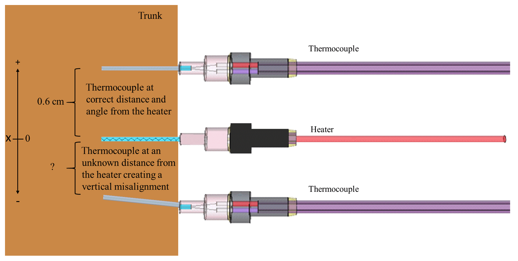
Figure 1 Schematic drawing of the three probes used for the heat ratio method: two thermocouples and one heater. One thermocouple (top) demonstrates the correct placement and is aligned vertically and symmetrically at 0.6 cm from the heater. The other thermocouple (bottom) demonstrates misalignment, which occurs when the probe is closer to the heater and is not aligned symmetrically. The zero is marked at the height of the heater, indicating that the placement of the thermocouples is estimated in relation to the heater at a distance of 0.6 and −0.6 cm (as indicated by the arrows). Sensors are modified from Davis et al. (2012) with permission.

There are a range of techniques used to measure sap flow, with “method families” varying between heat dissipation (HD; Granier, 1987; Lu et al., 2004), stem heat balance (SHB; Langensiepen et al., 2014), trunk segment heat balance (THB; Smith and Allen, 1996) and heat pulse velocity (HPV; Marshall, 1958); however, they are all based on tracing heat within the xylem (Burgess et al., 2001; Davis et al., 2012; Forster, 2017). Marshall (1958) developed a theoretical method to determine sap flow from thermal diffusion and dissipation theory of heat pulses in wood. His technique relies on calculating the heat ratios measured in two parallel thermocouples aligned vertically and symmetrically with respect to a line heater along the direction of the xylem (Fig. 1). Burgess et al. (2001) developed an improved HPV technique, termed “the heat ratio method” (HRM), based on the methodology of Marshall (1958). The HRM is sensitive to the direction of the sap flow and is therefore able to measure low and reverse rates (Burgess et al., 2001). Thus, the HRM is more appropriate for use in water-deficient environments where flow rates are low. Burgess et al. (2001) developed a two-step correction for sap flow calculations by considering probe misalignment and wounding, both of which are caused by the implementation of the sensors (Fig. 1). By accounting for these sources of error and additionally estimating the stem moisture content and radial variability, the HRM has been evaluated as the HPV method with the highest accuracy, although it has a tendency to underestimate transpiration values (Forster, 2017) – an error that has been shown to increase with higher sap flow rates (Steppe et al., 2010).

Previous studies have suggested additional solutions for probe misalignment (Ren et al., 2017), for determining thermal diffusivity (Vandegehuchte and Steppe, 2012) and for correcting for the heterogeneous heat capacity in wood (Becker and Edwards, 1999). However, there is no recent recommendation regarding how long newly deployed sap flow sensors can be employed. Some studies have shown how sensor probes inserted into the xylem can dampen the signal due to the blockage or destruction of vessels (Moore et al., 2010; Wiedemann et al., 2016). One way to avoid changes over time has been to reinstall sensors during the study period (Moore et al., 2010), although this interrupts continuous measurements in long-term datasets (Moore et al., 2010). Furthermore, there is little information to be found regarding the exact time interval that should be used with respect to sensor reinstallation (Vandegehuchte and Steppe, 2013). Therefore, we aim to find a quality indicator that can ensure that readings do not deteriorate over time, or, if they do, that the deterioration would be detectable. Attention should be paid to checking the accuracy of the raw readings that the rest of the methodology is based on. In addition, to allow for sensors to be employed over longer periods, it is necessary to develop a dynamic probe misalignment correction method due to observed changes in probe position over time. The adjustment proposed here, which is built on the calculations of Burgess et al. (2001), is necessary when monitoring transpiration continuously for more than 3 months due to an observed shift in probe placement from one season to another (Figs. 4, 6). Wood properties, the heterogeneity of the xylem and plant tissue growth might further misplace the sensor after its implementation (Barrett et al., 1995). Burgess et al. (2001) corrected for linear probe misalignment in situ when an enforced zero sap flow was attained by severing root systems at the end of the experiment. However, this solution is not suitable for long-term measurements, as the misplacement will change over time (Ren et al., 2017), or when intrusive methods are not an option. Thus, the objectives of this research are (1) to develop a statistical filtering method to ensure the quality and consistency of the measurements over time, and (2) to implement a modified version of the probe placement calculation for sap flow series longer than 3 months.

This technical note is structured in two parts: the first section deals with the statistical analysis of long-term time series of averaged heat ratios to ensure the quality of data and their stability over time; the second section proposes an adaptation of the method developed by Burgess et al. (2001) to introduce a dynamic probe misalignment correction for the HRM. The aim is to obtain a more precise calculation of transpiration by parameterising the probe misalignment as a function of time to correct for the effect of tree growth.

2 Materials and methods

2.1 Field site

This study was carried out at an inland experimental plot located in the Turia River basin, eastern Spain (39^∘57^′45^′′ N, 1^∘8^′31^′′ W), which experiences a Mediterranean climate with continental features. Average annual rainfall is 475 mm yr⁻¹, and the average annual maximum and minimum temperatures are 15.5 and 4.4 ^∘C respectively. Sap flow sensors were installed in four pine trees (Pinus halepensis Mill.) according to the heat ratio method (HRM; Burgess et al., 2001). Each sap flow sensor consisted of three needles: one heater and two thermocouples. We will refer to the thermocouples as probes, and the term “sensors” will be used to refer to both probes and the heater. To establish a criterion that unified the effect of the hillslope, all sensors were drilled into the uphill side of each tree trunk. This was assumed to offer a greater consistency regarding soil water retention, which is possibly higher at this orientation. All sensors were covered with radiation shields. As P. halepensis has a higher sap velocity near the cambium that steadily declines nearer to the heartwood (Cohen et al., 2008), sensors were installed at a depth of ∼20 mm below the cambium to account for the average sap velocity rate, as estimated by Manrique-Alba (2017). A metal plate was used as a guide during installation to ensure 0.6 cm spacing between the drilled holes. The selected pines had an average diameter of 24.5 cm at breast height. Continuous measurements were obtained from April 2017 to December 2018.

2.2 Environmental conditions

Air relative humidity (%) and air temperature (^∘C) were registered every 30 min (U23 Pro v2, Onset Computer Corporation, USA). Precipitation was registered using a rain gauge with a 0.2 mm resolution (RG3-M, Onset Computer Corporation, USA). Three soil moisture probes were inserted at a depth of 20–25 cm to register soil water content (SWC; S-SMD-M005, Onset Computer Corporation, USA), using a datalogger for data sampling and measurement recording (HOBO Micro Station, USA). To assume periods of zero sap flow, relative extractable water (REW) was calculated using the method of Bréda et al. (1995):

$$\begin{array}{}\text{(1)}& \mathrm{REW}={\displaystyle \frac{\left({\mathit{\theta }}_t-{\mathit{\theta }}_{min}\right)}{\left({\mathit{\theta }}_{max}-{\mathit{\theta }}_{min}\right)}},\end{array}$$

where θ_t is the registered SWC, θ_min is the minimum SWC observed during the measurement period and θ_max is the SWC at field capacity. Values surpassing one were converted to one, according to Granier et al. (2000).

2.3 Construction of the sensors

The thermocouples were made following Davis et al. (2012), using a type E junction of chromium and constantan. The wires of the thermocouples were soldered together at temperatures not surpassing 200 ^∘C, placed 20 mm inside a micropipette (10 µL) and then placed into a needle (0.12 cm × 4 cm, Sterican, Braun). The heater was made from a 20 mm constantan wire that was coiled around a 7 cm long aluminium wire and placed inside the same type of needle as the thermocouples. The wire ends were then soldered onto an electrical cable. A resistance of 4.95 Ω was then soldered onto to the cable to get a total electrical resistance of 14.95 Ω. The heater was connected via a solid-state relay to a 12 V battery, delivering 7.0 W of power when emitting heat pulses. Both thermocouples were connected to a CR800 datalogger for measurement recording (Campbell Scientific Inc., USA).

2.4 Quality control

Marshall (1958) parameterised the instantaneous heat pulse velocity (V) in the HRM as a function of time (s) following a heat pulse as well as an instantaneous heat pulse ratio (HPR), defined as HPR $=\frac{v_{\mathrm{1}}}{v_{\mathrm{2}}}$, where v₁ and v₂ are the respective downstream and upstream temperature increases measured after the release of a heat pulse:

$$\begin{array}{}\text{(2)}& V={\displaystyle \frac{\mathrm{4}Kt\ln \left(\frac{v_{\mathrm{1}}}{v_{\mathrm{2}}}\right)-\left(x_{\mathrm{2}}^{\mathrm{2}}+y_{\mathrm{2}}^{\mathrm{2}}\right)+\left(x_{\mathrm{1}}^{\mathrm{2}}+y_{\mathrm{1}}^{\mathrm{2}}\right)}{\mathrm{2}t\left(x_{\mathrm{1}}-x_{\mathrm{2}}\right)}},\end{array}$$

Here K is the thermal diffusivity (cm² s⁻¹), t is the time passed from the release of thermal pulse (s), and (x₁, y₁) and (x₂, y₂) are the relative positions (cm) of the thermocouples to the heater (considering the x axis along the xylem and the y axis in the perpendicular direction); see Fig. 2.

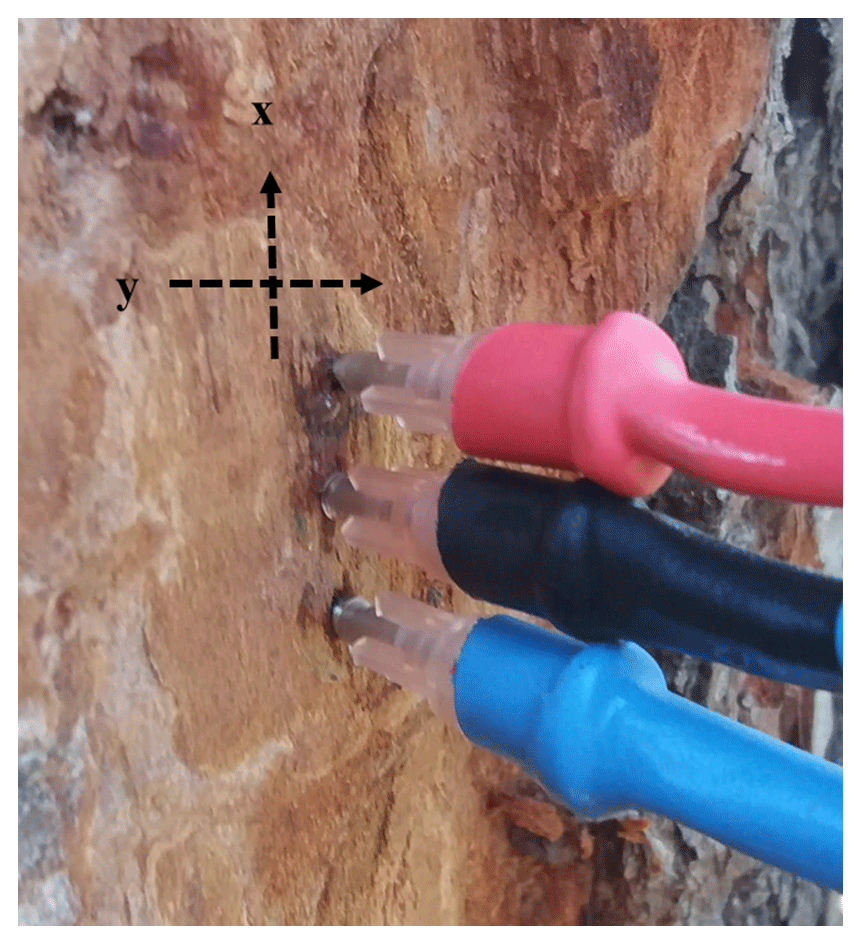
Figure 2 Sensor placements, showing (from top to bottom) the downstream thermocouple, heater and upstream thermocouple, in an Aleppo pine. The x axis represents sap flow direction and the vertical distance from the heater, and the y axis accounts for the horizontal probe distance from the x axis. The axes should cross where the heater is inserted but are displaced for a clearer view of the coordinates.

If the probes are installed equidistant to the heater and aligned along the vertical axis, $x=x_{\mathrm{1}}=-x_{\mathrm{2}}$ and $y_{\mathrm{1}}=-y_{\mathrm{2}}=\mathrm{0}$; Eq. (2) simplifies this into a function that is independent of time:

$$\begin{array}{}\text{(3)}& \begin{array}{rl}& V=\mathit{\varphi }\ln \left({\displaystyle \frac{v_{\mathrm{1}}}{v_{\mathrm{2}}}}\right)\\ & \mathit{\varphi }={\displaystyle \frac{K}{x}},\end{array}\end{array}$$

where ϕ is a priori constant that only depends on the placement of the probes and on the thermal diffusivity of both the xylem and the material used in the sensors, and x is a positive magnitude representing the distance from the heater element for the two probes.

For a whole sequence of instantaneous measurements, which typically comprises one measurement per second from the 60th second to the 100th second after a heat pulse release, the above equation should provide a heat pulse velocity that is slightly dependent on time, as provided by Burgess et al. (2001), when the wound width and sap velocities are small, with some inherent departures that are explained by instrumental errors alone. The “perfect symmetry” assumption renders that the heat pulse ratio remains constant with time if the heat pulse velocity (V), the thermal diffusivity (K) and the probe positions (in both the x and y directions) have negligible variations during the time following each heat pulse (Marshall, 1958). Burgess et al. (2001) further demonstrated how empirical results initially differed from the ideal approach described by Eq. (3) due to the blockage of xylem vessels and probe misplacement. However, the study concludes that the HPR converges asymptotically to a slightly tilted straight line at least 60 s after the heat pulse release and for at least 40 s more (until 100 s after the heat pulse release), which is when the instantaneous heat pulse ratio should be measured because the temperature stabilises at this point. Our study argues that a visual inspection of heat pulse velocities (V in Eqs. 2 and 3) does not necessarily give enough information to decide if measured values are a good representation of the sap flow. The method does not consider that measurement errors can arise, which is likely to occur in practice due to the sensitivity of the method. On these premises, we have built a methodology to quality control sap flow measurements systematically by introducing a statistical analysis performed on the instantaneous heat pulse ratio, which is acquired between 60 and 100 s after the heat pulse release. Hereafter, we will denote the averaged heat pulse ratio between 60 and 100 s as HPR. The quality control consisted of establishing threshold values for the slope of the HPR against time and the relative standard deviation (RSD), which was statistically defined as the standard deviation divided by the mean. The statistical information obtained would account for any deterioration in the measurement. Burgess et al. (2001) proposed two separate methods to correct for wounding and misalignment. The methods assume that errors arising from the wound inflicted by a sensor probe can be estimated using an empirical factor, whereas a misalignment of the probe needs to be calculated in situ. We propose the development of a misalignment correction method, while arguing that a statistical check of the HPR values would detect a deterioration in the signal caused by a worsening of the wound. Therefore, the RSD was chosen as a quality control parameter in addition to the slope, which was a parameter proposed by Burgess et al. (2001).

2.5 Logging specifications

The proposed analysis to ensure the reliability of long time series of sap flow measurements requires the storage of statistics that are not usually recorded (as they are considered unnecessary). The datalogger must have minimum capabilities with respect to the storage capacity (memory) and the processing speed of the algorithm implemented (especially in the routines related to the statistical calculations to be performed). In this study, a CR800 datalogger (Campbell Scientific, USA) was used. A flow chart of the sampling procedure and the datalogging commands (Fig. S1 in the Supplement) was specifically designed, programmed and implemented in the datalogger to enable the calculations that are presented in the next sections of this paper.

Figure 3 (a) Heat pulse ratios (HPRs) throughout the measurement period at 30 min intervals in pine 1. Each HPR is an average of 41 instantaneous ratios corresponding to the temperature difference in two thermocouples at 0.6 cm up- and downstream of a heater element at a depth of 2 cm. (b) Zoomed in panel of HPR data for 1 week of measurements to better see the diurnal pattern. (c) The relative standard deviation (RSD; %) for each HPR in pine 1 for the whole measurement period. The red line indicates the threshold used for the quality control: all HPR with a RSD >5 % were removed from the data analysis. (d) Zoomed in panel of RSD data for 1 week. (e) Slope (s⁻¹) for each HPR in pine 1 for the whole measurement period. The red line indicates the threshold used for the quality control for this particular sensor. All data above or below these lines are filtered out, as they did not correspond to HPR with $|\mathrm{slope}-\mathrm{median}(\mathrm{slope}\left)\right|<\mathrm{0.003}$ s⁻¹. The median slope for this sensor was −0.004 s⁻¹. (f) Zoomed in panel of slope data for 1 week of measurements.

We selected the RSD (%) and slope (s⁻¹) of the instantaneous heat pulse ratio versus time, calculated for each of the periods from 60 to 100 s, to filter out measurement errors (Fig. 3). The HPR should be close to constant during this period and should have a small slope value. Deviations from an idealised slope (positive or negative) mean that the HPR does not remain constant with time. All HPRs with a RSD >5 % and a $|\mathrm{slope}-\mathrm{median}(\mathrm{slope}\left)\right|>\mathrm{0.003}$ s⁻¹ were removed in order to filter out measurements with large variability in the slope, i.e. with large deviation from the ideal slope at this velocity. The 5 % threshold was chosen to ensure that 95 % of the dataset could be considered in the data processing. The slope median was taken from all slope values obtained during the measurement period. The magnitude of the threshold chosen for the slope was taken from a modelled output of instantaneous ratios performed by Burgess et al. (2001), where low sap flow velocities (5 cm h⁻¹) combined with a small wound width (0.17 cm) were shown to display a slope of 0.001. Due to our low sap flow velocities (<8 cm h⁻¹) and small probe diameter (0.12 cm), we expected the slope to be close to 0.001. The specific threshold of 0.003 was chosen upon inspection of the measurements and can be modified according to the needle size and the magnitude of the sap velocity measured. According to Burgess et al. (2001), higher slope values (0.01) can be expected with larger wound widths and higher velocities.

2.6 Correction for long-term probe misplacement

Under the assumption of “perfect symmetry”, in periods when V=0 cm h⁻¹, the HPR would be equal to one (v₁=v₂ in Eq. 3). However, this is not always the case with field measurements due to misalignment of the probe, damage to xylem vessels when inserting the probes, and the different thermal properties of the wood and needle. Burgess et al. (2001) proposed a methodology applied to in situ HRM measurements to account for this type of probe misalignment, building on the assumption that errors arising from inaccurate probe spacing can be treated one-dimensionally. This approach assumes that the total effect of probe misalignment (in both axes' directions), observed in the ratio of the increase in temperature, can be parameterised by calculating an “effective” probe misalignment in only one direction (in the x direction – parallel to the xylem). Thus, without the assumption of “perfect symmetry”, in periods when V=0 cm h⁻¹, Eq. 2 takes a more simplified form:

$$\begin{array}{}\text{(4)}& \mathrm{4}Kt\ln \left({\displaystyle \frac{v_{\mathrm{1}}}{v_{\mathrm{2}}}}\right)=\left(x_{\mathrm{2}}^{\mathrm{2}}+y_{\mathrm{2}}^{\mathrm{2}}\right)-\left(x_{\mathrm{1}}^{\mathrm{2}}+y_{\mathrm{1}}^{\mathrm{2}}\right),\end{array}$$

which becomes

$$\begin{array}{}\text{(5)}& \mathrm{4}Kt\ln \left({\displaystyle \frac{v_{\mathrm{1}}}{v_{\mathrm{2}}}}\right)=x_{\mathrm{2}}^{\mathrm{2}}-x_{\mathrm{1}}^{\mathrm{2}}\end{array}$$

if $y_{\mathrm{1}}=-y_{\mathrm{2}}$ or y₁=y₂.

As it is unknown if the misalignment is in x₁ or in x₂, the calculation is repeated twice in the present study, assuming first that x₁ is correct when estimating x₂ placement, and vice versa. Both x₁ and x₂ may be considered slightly misaligned, but, in this approximation, each of the two correction steps will assume that the other probe is correctly placed. The average of the obtained misalignments calculated for each of the probes will be considered as the resulting misalignment sought (Burgess et al., 2001). Each probe placement is calculated as follows:

$$\begin{array}{}\text{(6)}& x_{\mathrm{2}}=\sqrt{\left(\mathrm{4}kt\ln \left({\displaystyle \frac{v_{\mathrm{1}}}{v_{\mathrm{2}}}}\right)+x_{\mathrm{1}}^{\mathrm{2}}\right)}\end{array}$$

Therefore, two different heat pulse velocities, V₁ and V₂, are derived (using Eq. 2 but with the assumptions y₁=y₂ or $y_{\mathrm{1}}=-y_{\mathrm{2}}$) for the x₁ and x₂ obtained; the final V provided is their average.

Zero-flow conditions can either be imposed artificially by severing the root or stem (Burgess et al., 2001), or they can be found when there is no biophysical driving force (Forster, 2017). These conditions are accomplished when the atmospheric vapour pressure deficit (VPD) is close to zero, soil is saturated (usually after substantial precipitation) and measurements are taken predawn (Forster, 2017). Zero-flow conditions were assumed at night (22:00–03:00 UTC, coordinated universal time) during days when the REW was greater than 0.75 and the vapour pressure deficit (VPD) was close to zero (Fig. S2). Multiple readings were used to produce an average of each event. These conditions were limited to five occasions during the study period. Saturated soil is a necessary criterion due to the possibility of reverse flow at night-time (Forster, 2014). If not considered, low HPR values representing reverse flows can be interpreted as zero flow. If several calculations of x₁ and x₂ (Eq. 6) are performed during long monitoring periods, the nonintrusive approach of zero flow allows for the parameterisation of misalignment as a function of time (Eq. 7). By applying Eq. (6) at various times throughout the measurement period, it is possible to calculate a linear regression using the estimation of Burgess et al. (2001) for the obtained misalignments for each of the probes:

$$\begin{array}{}\text{(7)}& \begin{array}{rl}& x_{\mathrm{1}}=m_{\mathrm{1}}d+n_{\mathrm{1}}\\ & -x_{\mathrm{2}}=m_{\mathrm{2}}d+n_{\mathrm{2}},\end{array}\end{array}$$

where d is the time along the measuring campaign in days, x₁ and x₂ are the positions of the probes relative to the heater element in centimetres, m₁ and m₂ are the slopes, and n₁ and n₂ are the interception coefficients of the linear regressions for probes 1 and 2 respectively. The negative sign in front of x₂ in Eq. (7) is to clarify that this probe needs a negative root square solution.

By introducing Eq. (7) in Eq. (2) and allowing the simplification y₁=y₂ or $y_{\mathrm{1}}=-y_{\mathrm{2}}$, two equations of the corrected heat pulse velocities are obtained as a function of the time during the measuring field campaign:

$$\begin{array}{}\text{(8)}& \begin{array}{rl}& V_{\mathrm{1}}={\displaystyle \frac{\mathrm{4}Kt\ln \left(\frac{v_{\mathrm{1}}}{v_{\mathrm{2}}}\right)+{\left(m_{\mathrm{1}}d+n_{\mathrm{1}}\right)}^{\mathrm{2}}-{\mathrm{0.6}}^{\mathrm{2}}}{\mathrm{2}t\left(m_{\mathrm{1}}d+n_{\mathrm{1}}+\mathrm{0.6}\right)}}\\ & V_{\mathrm{2}}={\displaystyle \frac{\mathrm{4}Kt\ln \left(\frac{v_{\mathrm{1}}}{v_{\mathrm{2}}}\right)+{\mathrm{0.6}}^{\mathrm{2}}-{\left(m_{\mathrm{2}}d+n_{\mathrm{2}}\right)}^{\mathrm{2}}}{\mathrm{2}t\left(\mathrm{0.6}+m_{\mathrm{2}}d+n_{\mathrm{2}}\right)}}\end{array}\end{array}$$

In accordance with what Burgess et al. (2001) proposes, our approach averages the two values obtained from Eq. (8) to estimate a corrected heat pulse velocity.

3 Results

3.1 Heat pulse ratios

The HPR obtained during the measurement period displayed a clear positive shift away from the theoretical ideal where the HPR would equal one at zero flow (Fig. 3a). This gives an indication of the necessity of corrections for the wound inflicted by the probe, misalignment, and misestimation of thermal diffusivity or stem water content. However, the HPR data themselves do not give an indication of the quality of each measurement nor if the quality of the measurements deteriorates over time. Therefore, the quality of the measurements was indicated by calculating the RSD and the slope associated with each HPR (Fig. 3c, d, e, f). All HPRs with a RSD value higher than 5 % were eliminated. The data points eliminated corresponded to 1 % of the total dataset. Because the HRM is built on the theoretical assertion that the instantaneous HPR is close to linear with time and slightly tilted, specifically between 60 and 100 s after the release of a heat pulse, the slope of the HPR should be small, although it should also be dependent on the sap velocity and wound width (Burgess et al., 2001). Our HPR dataset displayed slope values close to what Burgess et al. (2001) proposed, but there were also measurements where the slope varied substantially; thus, we decided to filter out HPRs with $|\mathrm{slope}-\mathrm{median}(\mathrm{slope}\left)\right|>\mathrm{0.003}$ s⁻¹. This corresponded to 12 % of the original dataset (Fig. 3e, f).

3.2 Heat pulse velocities

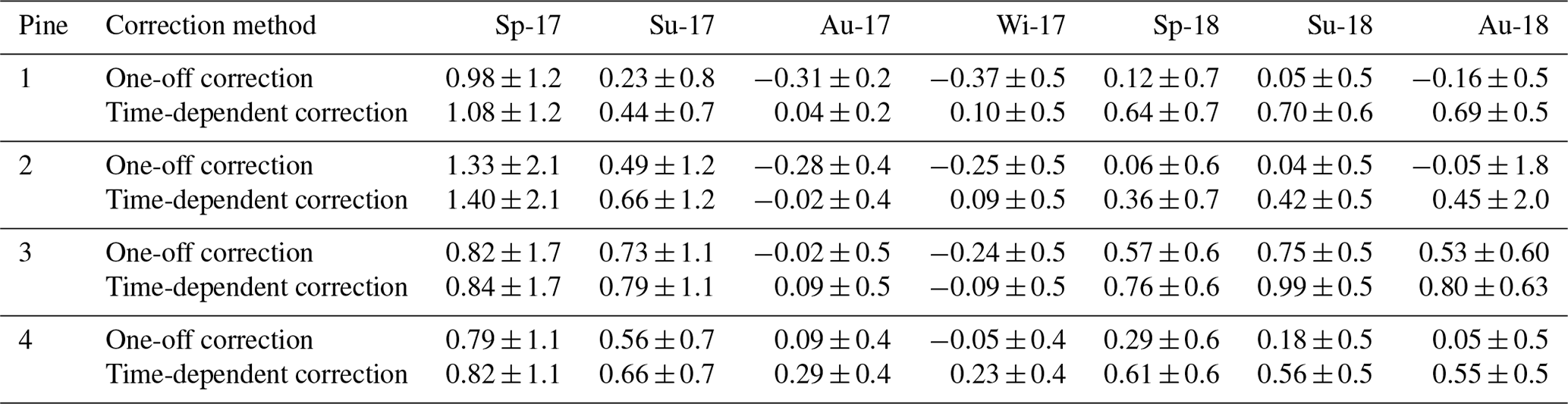
A linear regression was obtained from misalignment calculations for each sensor performed during zero-flow conditions. Zero-flow conditions were assumed at night (22:00–03:00 UTC) during periods when the REW was greater than 0.75 and the vapour pressure deficit (VPD) was close to zero (Fig. S2). Multiple readings were used to produce an average of each event. These conditions were limited to five occasions during the study period. The outputs indicate a clear shift in the placement of each of the sensors over time, here denoted as x₁ and x₂ in each tree (Fig. 4). The eight probes, two per tree, all deviated from the ideal of 0.6 cm. Probe x₂ in pine 1 had the highest inaccuracy, with an initial value close to 0.3 cm. On average, the probes showed a shift of 0.04 cm in placement after 20 months of measurement (Fig. 4). The equation obtained from the linear regression was then implemented in Eq. (8), and corrections of the heat pulse velocity data were carried out using an average of V₁ and V₂ (Fig. 5). Outputs were compared with one-off misalignment corrections, which were calculated at the beginning of the measurement period to demonstrate the evolution of the probe misalignment. The one-off correction demonstrated a steady decline in accuracy over time (Fig. 5). The difference between the two correction methods showed significance after 3 months of employment (Table 1).

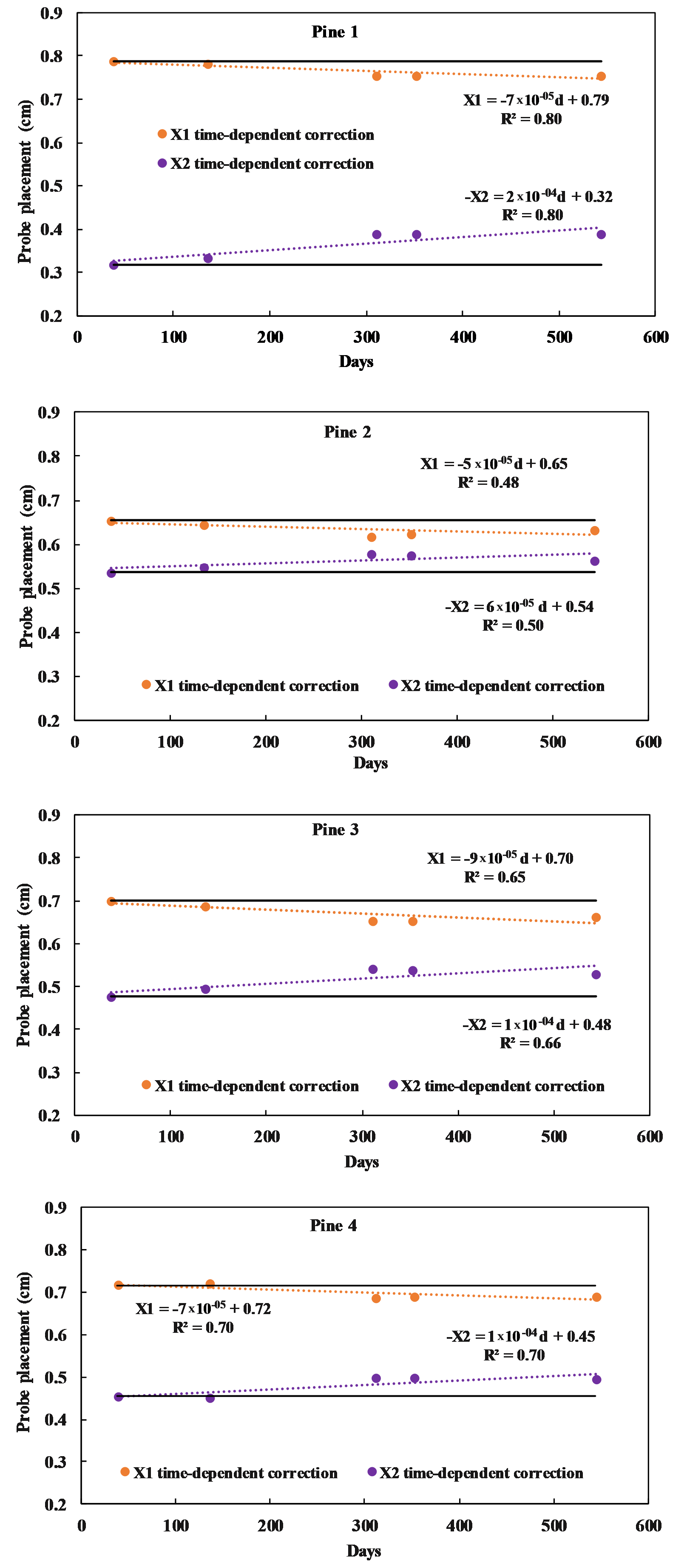
Figure 4 The placement of the probes is shown as a distance from the heater (cm). Probe placement was calculated once at the beginning of the measurement period (solid lines) for the whole study period and compared to probe placement calculated at various times (solid circles with dotted lines) during the study period. Each point represents the probe position calculated during its respective zero-flow event.

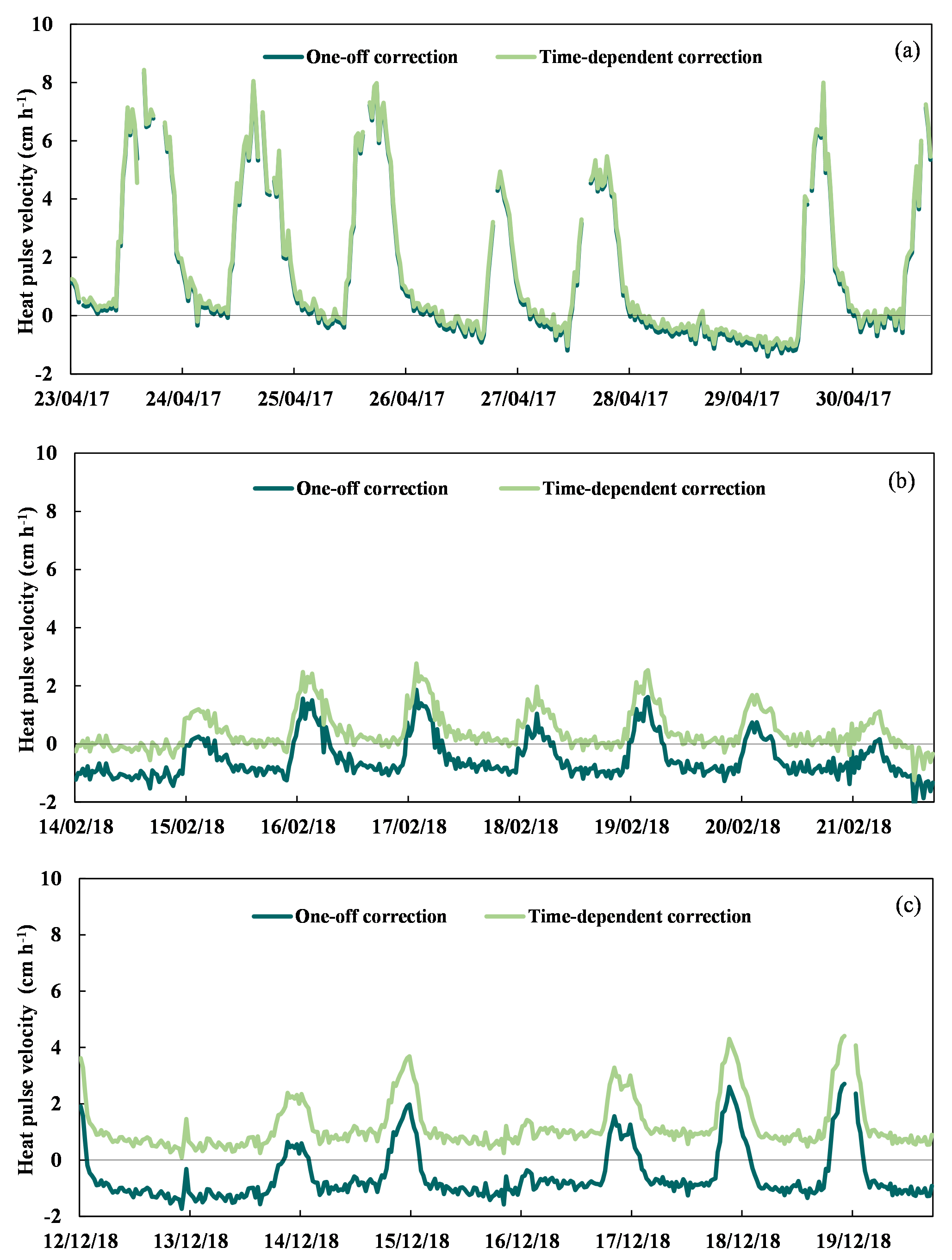
Figure 5 Heat pulse velocities during 1 week of measurements at the beginning (a), halfway through (b) and at the end (c) of the measurement period. Dark green lines represent velocities with probe misalignment corrected for once at the beginning of the experiment. Light green lines represent velocities with the time-dependent probe misalignment corrections.

Table 1 Seasonal averages of sap velocity for four different pines. All sap flow values are expressed in cubic centimetres per square centimetre per hour (cm³ cm⁻² h⁻¹). Sap flow values corrected for with time-dependent misalignment calculations are compared with sap flow values corrected for once at the beginning of the measurement period. Averages were taken from daily values. Sp, Su, Au and Wi indicate spring (March–May), summer (June–August), autumn (September–November) and winter (December–February) respectively; the corresponding year for each season is shown following the hyphen.

3.3 Sap flow

Heat pulse velocities (cm h⁻¹) were converted into sap flow (cm³ cm⁻² h⁻¹) according to Burgess et al. (2001). Our data demonstrated that by not correcting for changes in probe misalignment under continuous measurement for more than 3 months, the errors corresponded to an averaged difference of 0.29 (cm³ cm⁻² h⁻¹) in sap flow per quarter for the four trees. At the end of the 20-month period, this corresponded to an averaged difference of 0.53 (±0.23) cm³ cm⁻² h⁻¹ (Table 1, Fig. 6). In terms of transpiration values, this corresponded to a mean difference of 0.7 L tree⁻¹ d⁻¹ (sapwood area of 170 cm²), which would correspond to a difference of 542 L ha⁻¹ d⁻¹ (775 tree ha⁻¹) assuming 8 h of daylight. It is relevant to note that our conversion did not consider the differences in stem moisture content, which can also affect the output values (Vandegehuchte and Steppe, 2013). The outputs obtained should be considered as relative differences, as the one-off correction was applied at the beginning of the experiment.

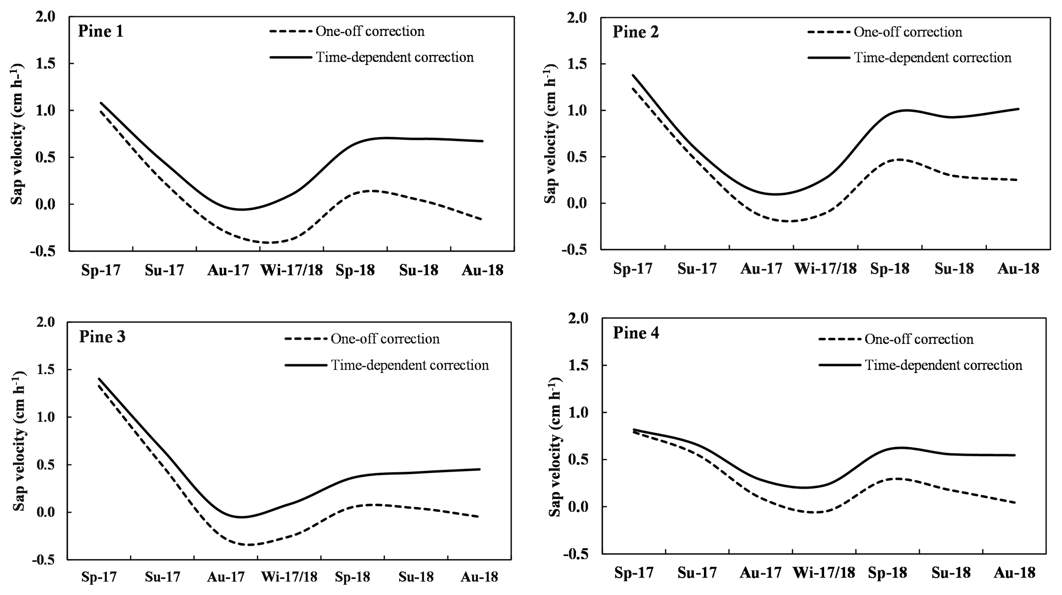
Figure 6 Seasonal averages of sap flow (cm³ cm⁻² h⁻¹) calculated using the two misalignment corrections during the 20-month measurement period. Dotted lines represent probe misalignment that was corrected for once. Solid lines represent sap flow that was corrected for using the time-dependent probe misalignment method. Sp, Su, Au and Wi indicate spring (March–May), summer (June–August), autumn (September–November) and winter (December–February) respectively; the corresponding year for each season is shown following the hyphen.

3.4 Transpiration

To demonstrate the difference in terms of transpiration, sap flow values (cm³ cm⁻² h⁻¹) without misalignment correction (T), with the one-off correction (T_one) and with the time-dependent correction (T_time) were converted into transpiration values (L tree⁻¹ h⁻¹) and compared against each other over a period of 3 weeks. Data from three of the pines (1, 3 and 4) were taken towards the end of the measurement period in order to demonstrate the greatest differences (Fig. 7). However, the sensor placement in pine 2 displayed a misplacement closer to target (0.6 cm) towards the end of the measurement period (Fig. 4); therefore, and another measurement period was chosen for this pine in order to better demonstrate the differences between the estimations. Note that the transpiration estimations without misalignment correction still went through the wound correction step as shown in Burgess et al. (2001). Pine 1 displayed the biggest differences between T and T_time, with an average daily difference of 1.5±0.002 (L tree⁻¹) during the 3 weeks and a difference in the daily average of 0.3±0.003 (L tree⁻¹) between T_one and T_time. Pines 3 and 4 showed similar differences between the methods, with a respective daily average of 0.1±0.001 and 0.2±0.002 (L tree⁻¹) between T and T_time. Both had a difference in the daily average of 0.1±0.001 (L tree⁻¹) between T_one and T_time (Fig. 7).

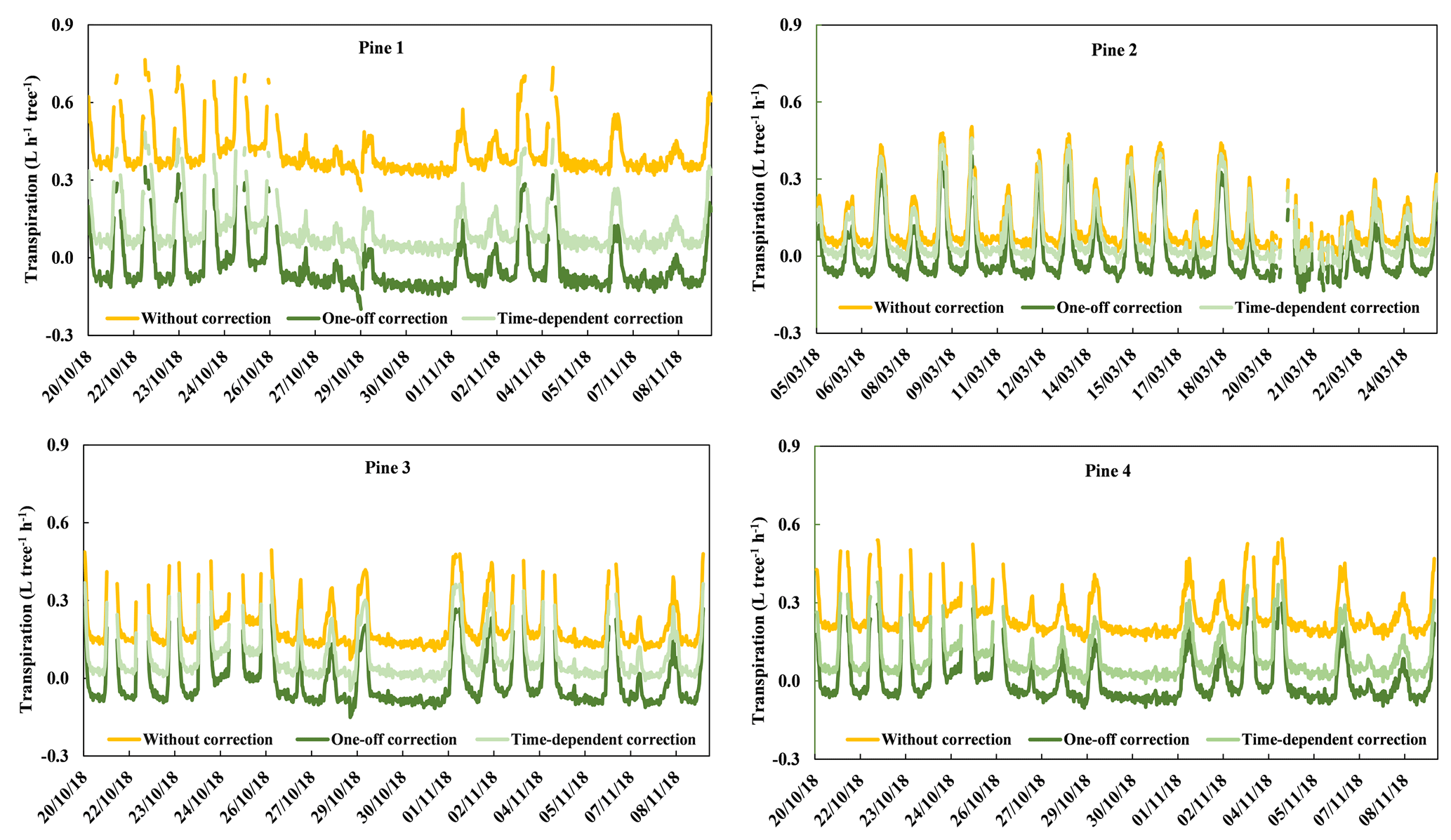
Figure 7 The 3 weeks of transpiration rates (L tree⁻¹ h⁻¹). “Without correction” represents rates without misalignment corrections, “One-off correction” represents rates that were corrected for once at the beginning of the measurement period and “Time-dependent correction” represents rates that were corrected for on various days throughout the measurement period.

4 Discussion

4.1 Filtering heat pulse ratios

Because the HPR is an average of the instantaneous temperature difference ratios, it is difficult to ensure its accuracy by visual inspection of the averaged output alone and without further statistical information. For each heat pulse measurement sequence, we suggest a RSD and slope from the linear regression of the instantaneous ratios versus time in order to filter out erratic measurements and to ensure the quality of the data. When this procedure is considered for long time field measurements, a clear tendency may be observed toward higher RSD and slope values during periods with higher flow rates (Fig. 3), indicating more noise and less trustworthy data during these episodes. The HRM only measures values below 45 cm h⁻¹ (Forster, 2017), due to a maximum $\frac{v_{\mathrm{1}}}{v_{\mathrm{2}}}$ ratio of 20, as this is the range within which the ratio can be assumed accurate (Burgess et al., 2001; Marshall, 1958). Because our dataset showed no velocities higher than 8 cm h⁻¹, it was not initially considered a limitation for the measurements.

During the 20 months of field measurements, the thermocouples showed no visible sign of deterioration with time. However, it is still important to note that this does not take the possible diminishing amplitude of the ratios over time into account, which can also lead to underestimations of actual flow (Barett et al., 1995; Green et al., 2003; Forster, 2017). Therefore, this should be observed separately by comparing sap flow ratios using data obtained under similar climatic conditions (Moore et al., 2010). Due to the variation in rainfall between the 2 years, the SWC differed significantly on similar calendar dates apart from 6 d in June (9–15 June). When comparing the relationship of sap flow versus VPD on these days, there was an increase in the slope: 2.3 for 2017 and 2.9 for 2018. We attributed this to an overall weaker correlation between the VPD and sap flow in 2017 (R²=0.4 in 2017 versus R²=0.6 in 2018), due to higher VPD values the first year (Fig. S3). In conclusion, it was clear that the HPR readings had not decreased in the second year, when compared to the first year, under similar environmental conditions.

4.2 Long-term variation in probe placement

When applying the HRM for longer than a few weeks, it is relevant to quantify how ϕ in Eq. (3) and the misalignment term in Eq. (5) evolve during the measuring period. The predicted variation of x₁ and x₂ is due to the growth of the tree as well as periodical variations in K due to annual and seasonal variations of the physiological properties of the tree (Green et al., 2003; Vandegehuchte and Steppe, 2012; Ren et al., 2017). In the HRM, the probe misalignment calculations can be corrected using the methodology proposed here, considering that each sensor displayed an average 0.04 cm displacement within the tree after 20 months of measurements. The correction would also be more rigorous with added zero-flow events, which would be easier to obtain in humid environments with more periods of saturated soil.

The theory behind the HPV method was tested on conifers (Marshall, 1958), whereas Burgess et al. (2001) more generally refers to woody species when working with the HRM. The time-dependent correction method could be useful for any species that has already been tested with the HRM, where the misalignment of probes can create a source of error and the sensors are installed over a longer period. Specifically, where the movement of the wood might cause further displacement of the sensor.

By going back to the original assumption of “perfect symmetry”, we investigated the original premises that the method is built upon. Even though Burgess et al. (2001) elaborated a correction method for sensor misalignment, we saw that changes in sensor placement were detectable after each season. Therefore, multiple corrections should be carried out during the measurement period. The proposed modified method coincides with the one-off correction method (Burgess et al., 2001) for short time periods (<3 months) but differs progressively over time. We found that this shift in placement is already significant after 3 months; therefore, dynamic misplacement calculations should be carried out or sensors should be reinstalled at this frequency. However, as pointed out by Moore et al. (2010), reinstalling the sensors might create a shift in the data due to spatial variation within the tree. Leaving the same sensors in the tree throughout the study period avoids this problem and enables the study to focus on the intrinsic factors affecting the sap flow rates.

5 Conclusion

In conclusion, we found that high quality measurements with sap flow sensors can be ensured over longer periods (>3 months) if the HPR is assessed using the proposed filtering method and the probe misalignment variability over time is corrected for. In this study, we observed data over a 20-month period in Pinus halepensis trees, and we saw no sign of deterioration in the second year compared to the first when observing the slope and RSD values obtained. However, when observing the alignment of each probe, there was a clear shift from the beginning to the end of the measurement period. This indicates that measurements can be obtained during a second season without the need to reinstall sap flow sensors if the proposed time-dependent misalignment correction is incorporated into the data processing. This would increase the accuracy of point measurements and, consequently, transpiration estimations. The different errors related to upscaling are beyond the scope of this paper, but significant differences were observed when comparing sap flow estimations with no correction, one-off correction and time-dependent correction for probe misalignment.