the Creative Commons Attribution 4.0 License.
the Creative Commons Attribution 4.0 License.
 | 26 May 2020
A daily 25 km short-latency rainfall product for data-scarce regions based on the integration of the Global Precipitation Measurement mission rainfall and multiple-satellite soil moisture products
Christian Massari
Luca Brocca
Thierry Pellarin
Gab Abramowitz
Paolo Filippucci
Luca Ciabatta
Viviana Maggioni
Yann Kerr
Diego Fernandez Prieto
Rain gauges are unevenly spaced around the world with extremely low gauge density over developing countries. For instance, in some regions in Africa the gauge density is often less than one station per 10 000 km2. The availability of rainfall data provided by gauges is also not always guaranteed in near real time or with a timeliness suited for agricultural and water resource management applications, as gauges are also subject to malfunctions and regulations imposed by national authorities. A potential alternative is satellite-based rainfall estimates, yet comparisons with in situ data suggest they are often not optimal.
In this study, we developed a short-latency (i.e. 2–3 d) rainfall product derived from the combination of the Integrated Multi-Satellite Retrievals for GPM (Global Precipitation Measurement) Early Run (IMERG-ER) with multiple-satellite soil-moisture-based rainfall products derived from ASCAT (Advanced Scatterometer), SMOS (Soil Moisture and Ocean Salinity) and SMAP (Soil Moisture Active and Passive) L3 (Level 3) satellite soil moisture (SM) retrievals. We tested the performance of this product over four regions characterized by high-quality ground-based rainfall datasets (India, the conterminous United States, Australia and Europe) and over data-scarce regions in Africa and South America by using triple-collocation (TC) analysis. We found that the integration of satellite SM observations with in situ rainfall observations is very beneficial with improvements of IMERG-ER up to 20 % and 40 % in terms of correlation and error, respectively, and a generalized enhancement in terms of categorical scores with the integrated product often outperforming reanalysis and ground-based long-latency datasets. We also found a relevant overestimation of the rainfall variability of GPM-based products (up to twice the reference value), which was significantly reduced after the integration with satellite soil-moisture-based rainfall estimates.
Given the importance of a reliable and readily available rainfall product for water resource management and agricultural applications over data-scarce regions, the developed product can provide a valuable and unique source of rainfall information for these regions.
- Article
(11289 KB) - Full-text XML
-
Supplement
(3742 KB) - BibTeX
- EndNote


Rainfall is the main driver of the hydrological cycle (Oki and Kanae, 2006) and plays an essential role in water resource management and agricultural applications (Vintrou et al., 2014; Gibon et al., 2018), drought monitoring (Garreaud et al., 2017) and flood forecasting (Maggioni and Massari, 2018).
Ground networks of rain gauges are considered the most accurate (and as a reflection the most used) rainfall observations across many regions of the world. However, the difficulty and the costs associated with their maintenance along with the timeliness of their data availability are critical obstacles for their use in real-time and seasonal applications. Moreover, while in developed regions the rain gauge distribution is sufficiently dense and supported by well-organized and well-funded organizations, in developing countries the data coverage is extremely poor.
The number of gauges around the world has been estimated to range between 150 000 and 250 000, but their distribution is far from being homogeneous (Kidd et al., 2017). For instance, in regions like Africa, South America and central Asia the gauge density is often less than one station per 10 000 km2, which results in large interpolation errors of gauge-based gridded rainfall products. This is an interesting paradox, since gauges are insufficient exactly where they are more needed. In these areas the only source of “observed” rainfall with a timeliness suited for applications is derived from satellite rainfall estimates (SREs) and meteorological models.
SREs are normally derived from sensors on board low-Earth-orbiting (LEO) and geostationary satellites (Kidd and Huffman, 2011; Serrat-Capdevila et al., 2014). While geostationary satellites use visible and infrared sensors to retrieve the precipitation signal with high spatial and temporal resolutions (e.g. 1–3 km and 15–30 min), low-Earth-orbiting satellites use passive microwave observations to provide global precipitation measurements with a frequency of about two observations per day with a spatial resolutions typically larger than 25 km. The latter are normally more accurate as they provide a more direct measurement of precipitation. A large number of techniques have been developed that exploit the synergy between polar-orbiting retrievals and geostationary observations (Huffman et al., 2007; Hsu et al., 1997; Joyce et al., 2004; Kubota et al., 2007).
The long history of research in the area led in 2014 to the Global Precipitation Measurement (GPM) mission (Hou et al., 2014), launched by NASA and JAXA (Japan Aerospace Exploration Agency) in coordination with the Goddard Earth Sciences Data and Information Services Center (GES DISC). The mission introduced a new concept for rainfall retrieval based on a multi-sensor integration. Within GPM, multiple observations from different instruments are intercalibrated, merged and interpolated with the GPM Combined Core Instrument product to produce half-hourly precipitation estimates on a 0.1∘ regular grid over the 60∘ N–S domain through the Integrated Multi-Satellite Retrievals for GPM (IMERG; Huffman et al., 2018). The mission provides three L3 (Level 3) products which are based on different level of timeliness and calibration configurations (the Early Run – IMERG-ER, the Late Run – IMERG-LR – and the Final Run – IMERG-FR; see Sect. 2.1.2 for further details).
Although extremely useful, one of the problems with SRE is the instantaneous nature of the measurement, which, along with the intermittent character of the rainfall, make SRE prone to errors (Kucera et al., 2013). For example, precipitation type and rate (Behrangi and Wen, 2017) along with satellite orbit and swath width (and thus the number of satellite snapshots available) all play an important role in determining the sampling error magnitude (Nijssen and Lettenmaier, 2004; Ciabatta et al., 2017b; Gebremichael and Krajewski, 2004). Other problems are associated with seasonally dependent biases, light rainfall estimation, and detection over snow- and ice-covered surfaces (Ferraro et al., 1994; Ebert et al., 2007; Kidd and Levizzani, 2011; Tian et al., 2007; Gottschalck et al., 2005). Although these problems have been reduced with the advent of the GPM mission thanks to the new Dual-frequency Precipitation Radar (DPR), recent works show that there is still room for improvement (Tan et al., 2016; O et al., 2017; Gebregiorgis et al., 2018b).
Model reanalysis datasets, such as the European Centre for Medium Weather Forecast (ECMWF) Interim Reanalysis (ERA-interim; extensively described in Dee et al., 2011) and the new ERA5 (European Centre For Medium-Range Weather Forecasts, 2017), are the obvious alternative to ground- and satellite-based rainfall products. Although they offer good performance in simulating synoptic weather systems, they often misrepresent the variability of convective systems, mainly due to their relatively low resolution and deficiencies in the parameterization of sub-grid processes (Roads, 2003; Ebert et al., 2007; Kidd et al., 2013; Beck et al., 2017). Although reanalysis datasets perform relatively well globally (Massari et al., 2017a) and provide consistent long-term precipitation estimation (which is paramount in many research fields), they are normally released with a latency that does not suit water resource and agricultural applications.
Despite these inherent limitations, SRE and reanalysis products are still the only valuable alternative to gauge-based observations within gauge-scarce regions, and the efforts to improve these datasets by merging procedures or by including other ancillary information has been significantly increasing in the last decade. For instance, Beck et al. (2017) released Multi-Source Weighted-Ensemble Precipitation (MSWEP), a dataset with a 3-hourly temporal resolution that covers the period 1979 to the near present. MSWEP is a unique product, as it exploits the complementary strengths of gauge-, satellite- and reanalysis-based data to provide rainfall estimates over the entire globe. Other notable examples are the CHIRPS (Climate Hazards Group Infrared Precipitation with Station data) rainfall estimates (Funk et al., 2015), which are based on a combination of gauges and infrared cold cloud duration (CCD) observations. However, these datasets rely upon the availability of gauge observations, which constitute the “land” or the “bottom-up” perspective of the precipitation signal (i.e. the precipitation that effectively reaches the land surface), in contrast to satellite (and reanalysis) estimates, which are more informative about the precipitation in the atmosphere layers (i.e. by cloud and atmospheric models). Where gauges are very sparse or totally missing or their functioning is not guaranteed in near real time, the quality of SRE and models can be significantly affected as the bottom constraint provided by gauges weakens.
A potential solution to circumvent this problem is the use of satellite SM observations as a source of rainfall ground information (Crow et al., 2009, 2011; Pellarin et al., 2008; Brocca et al., 2013; Pellarin et al., 2013; Wanders et al., 2015; Zhan et al., 2015; Ciabatta et al., 2015; Massari et al., 2019). In practice, SM can be used as a trace of precipitation, as the SM signal after a rain event persists from a few hours to several days. In other words, SM contains information about the amount of water stored in the soil after rainfall. This information can be then exploited to retrieve spatial and temporal characteristics of the precipitation that has effectively reached the land surface. For instance, Brocca et al. (2013, 2014) proposed a direct inversion of the soil water balance equation and used two consecutive satellite SM observations to estimate rainfall fallen within the time interval between the two satellite passes. The underlying idea of this method, known as SM2RAIN, is the use of “soil as a natural rain gauge”, as the difference in the water contained in the soil can be directly related to rainfall. This information was used to improve SRE by Ciabatta et al. (2017a) and Massari et al. (2019). Other techniques that exploited SM observations relied upon data assimilation approaches based on sequential filtering techniques, like Kalman-filter-based methods (Soil Moisture Analysis Rainfall Tool – SMART; Crow et al., 2011) and particle filters (Pellarin et al., 2013; Zhan et al., 2015; Román-Cascón et al., 2017). All of them demonstrated a real benefit for flood forecasting applications (Alvarez-Garreton et al., 2016; Chen et al., 2014; Massari et al., 2018). In all but two cases (Chen et al., 2014; Tarpanelli et al., 2017), one single SM product was combined with the SRE, a possible limitation if that product does not perform relatively well in the area of interest.
In general, the main advantage of using satellite SM as an indirect measure of ground rainfall information is its uniform temporal and spatial coverage, availability in near real time, and the fact that it transcends national boundaries. Drawbacks are the low spatial resolution and the relatively low quality in mountainous areas, frozen soils and dense forests, which, however, is also an issue in the case of ground-based observations (due to uneven spatial distribution and data transmission issues in inaccessible areas, undercatch problems, and the cost of maintenance). As these problems impact the type of the sensor (active or passive) and the retrieval in different way, their combination would allow for exploiting their relative strengths for improving SRE.
In this study, we developed a short-latency (2–3 d depending on the region) rainfall product derived from the combination of IMERG-ER with multiple-satellite SM-based rainfall products. The latter are obtained from the inversion of the SM retrievals derived from (1) the Soil Moisture Active and Passive (SMAP; Entekhabi et al., 2010) mission, (2) the Advanced Scatterometer (ASCAT; Wagner et al., 2013), and (3) the Soil Moisture and Ocean Salinity (SMOS; Kerr et al., 2001) mission via SM2RAIN. The integrated product is explicitly designed for operational water resource management and agricultural applications over data-scarce regions where rainfall observations from hydrometeorological networks are scarce or totally absent.
The integration method we adopted is the optimal linear combination (OLC) approach (Bishop and Abramowitz, 2013; Hobeichi et al., 2018), which is based on a technique that provides an analytically optimal linear combination of rainfall products and accounts for both the performance differences and error covariance between the products. We tested the performance of the product (1) over four key regions, namely, India (IN), the conterminous United States (CONUS), Australia (AU) and Europe (EU), where high-quality ground-based hydrometeorological networks are available, and (2) in Africa and South America by using a triple-collocation (TC) analysis (Stoffelen, 1998). The validity of TC and the consistency of its results with respect to those obtained against classical validation was preliminary tested over the four regions mentioned in point 1 (Massari et al., 2017a).
The key strengths of this integrated product are the following:
-
The simultaneous use of multiple-satellite SM observations derived from active and passive sensors. This exploits the advantages of each sensor in improving SRE. Note that ASCAT is on the Metop (Meteorological Operational) satellites, which are part of the space segment of the EUMETSAT (European Organisation for the Exploitation of Meteorological Satellites) Polar System (EPS) that will secure the continuation of meteorological observations from the polar orbit in the 2022–2043 timeframe.
-
The short latency (2–3 d, potentially lower in the near future and with Level 2 – L2 – products). This is of paramount importance for operational applications like flood forecasting (for medium to large catchments, i.e. >20 000 km2), water resource management, agricultural planning and vector-borne disease control.
-
Independence from rain gauge observations. This is a key factor for data-scarce regions like Africa.
The paper is divided as follows. Section 2 provides a brief overview of the ground-based and satellite observations used in the study. Section 3 describes algorithms and methods used as well as the integration methodology and the validation strategy. Results are presented in Sect. 4 followed by the discussion and conclusions.
In this section we describe the datasets used for the integration of IMERG-ER with SM2RAIN rainfall estimates, as well as the datasets used to validate the integrated product.
2.1 Regional rainfall datasets
Different ground-based rainfall datasets were used for the four different regions to cross-validate the integrated product, namely, the Australian Water Availability Project (AWAP) in Australia, the ECA&D (European Climate Assessment & Dataset) rainfall dataset E-OBS (ENSEMBLES daily gridded observational dataset) gridded dataset in Europe, the National Centers for Environmental Prediction (NCEP) Stage IV dataset over CONUS and the India Metrological Department (IMD) rainfall gridded dataset over India. Below we describe the main features of these datasets (readers interested in more details can refer to the related publications).
-
The Australian Water Availability Project (AWAP) rainfall product is generated via spatial analyses on the quality‐controlled daily rain gauge measurements from the Australian Bureau of Meteorology daily rain gauge network. AWAP daily rainfall for a given day is the 24 h total rainfall from the day before at 09:00 local time to the current day at 09:00. The rainfall fields are gridded on a grid and spatially resampled to the desired 0.25∘ grid by taking area‐weighted averages. Although this product is characterized by a relatively high quality, it suffers also from known shortcomings (the reader interested can refer to Contractor et al., 2015, for further details).
-
The ECA&D rainfall dataset E-OBS gridded dataset is derived through interpolation of the ECA&D (European Climate Assessment & Data) station data. The station dataset comprises a network of 2316 stations, with the highest station in northern and central Europe and lower density in the Mediterranean, northern Scandinavia and eastern Europe. The E-OBS dataset is derived through a three-stage process (Haylock et al., 2008), which brings it to different resolutions and grids. In this analysis, we used the 0.25∘ regular latitude–longitude grid.
-
The National Centers for Environmental Prediction (NCEP) Stage IV (Lin and Mitchell, 2005) is based on the Next Generation Weather Radar (NEXRAD) measurements, optimally merged with hourly gauge-based observations by using the Multisensor Precipitation Estimator (MPE; Seo et al., 2010). This hourly dataset has a spatial resolution of approximately 4 km. The hourly gauge observations in the NCEP Stage IV estimates are derived from the Hydrometeorological Automated Data System (HADS). Stage IV is characterized by a negligible amount (<1 %) of missing data over south-eastern CONUS, whereas about 90 % of the data are missing over the northwest corner of CONUS (roughly between 43–50∘ N and 115–125∘). In this study we aggregated the product by averaging all the 4 km pixels falling within the footprint. Daily data were obtained by the accumulation of hourly observations. In the accumulation procedure, if any missing hourly observations were found for the day, the resulting daily rainfall was discarded.
-
The India Metrological Department rainfall gridded dataset is prepared from daily rainfall data of 6955 stations, archived at the National Data Centre, IMD, Pune, by using the Shepard method (Pai et al., 2014). Out of these 6955 stations, 537 stations are the IMD observatory stations, 522 stations are under the hydro-meteorology programme and 70 are agrometeorological stations. Remaining stations are rainfall-reporting stations maintained by state governments. The product has been released with a spatial resolution since 1856.
2.1.1 Satellite soil moisture products
In the following we describe the main characteristics of the satellite SM products used in the study. They are the following:
-
The Advanced Scatterometer (ASCAT) on board the Metop-A, Metop-B and Metop-C satellites is a scatterometer operating at the C band (5.255 GHz). It provides a SM product characterized by a spatial sampling of 12.5 km and from one to two observations per day depending on the latitude (Wagner et al., 2013). In this study, the SM product provided within the EUMETSAT project (http://hsaf.meteoam.it/, last access: 24 April 2020) denoted as H115 was used.
-
The Soil Moisture and Ocean Salinity (SMOS) mission provides a SM product through a radiometer operating at the L band (1.4 GHz) with 50 km of spatial resolution and one observation every 2–3 d (Kerr et al., 2001). In this study, version RE04 (Level 3) provided by the Centre Aval de Traitement des Données SMOS (CATDS, https://www.catds.fr/, last access: 24 April 2020) was used. The version is gridded on the 25 km EASEv2 (Equal-Area Scalable Earth) grid and distributed in the netCDF (Network Common Data Form) format.
-
For SMAP L3, the Soil Moisture Active and Passive (SMAP) mission SM product is obtained by L-band radiometer observations (1.4 GHz) with 36 km and one or two observations every 3 d depending on the location (Entekhabi et al., 2010). In this study, the version 5 of the Level 3 SM retrievals was used.
-
For AMSR2, the Advanced Microwave Scanning Radiometer 2 (AMSR2) on board the Global Change Observation Mission for Water satellite is a radiometer operating in the microwave band. Soil moisture retrieval from AMSR2 is obtained from the C and X bands, which allow for obtaining a spatial–temporal resolution of 25 km daily (Kim et al., 2015). In this study, we focused on the X-band SM product obtained by the application of the Land Parameter Retrieval Model to AMSR2 brightness temperature data (Parinussa et al., 2015). Note that AMSR2 was inverted to obtain rainfall via SM2RAIN, but the resulting rainfall was not used in the integration, whereas it was used in the validation via TC as an auxiliary dataset.
2.1.2 Global rainfall datasets
In addition to satellite SM products, different rainfall datasets were used in the study both for cross-comparison purposes and as a part of the integration procedure. In the following the main characteristics of each dataset are provided.
-
The First Guess Daily product provided by the Global Precipitation Climatology Center (GPCC; Schamm et al., 2014) is a ground-based rainfall dataset, which has been available since 1 January 2009 with a spatial sampling grid of 1∘. This dataset is used within the processing chain of in many gauge-corrected satellite rainfall products. Being based on gauge observations, this dataset is very accurate where the station density is relatively high like in Europe, Australia and the United States, whereas it suffers from serious interpolation errors in areas uncovered by stations. For the sake of comparison, for GPCC we assumed the same rainfall observed at 1∘ on the sub-pixels.
-
ERA5 is the latest climate reanalysis produced by ECMWF, providing hourly data on many atmospheric, land-surface and sea-state parameters together with estimates of uncertainty. The rainfall variable used in this study is characterized by a spatial resolution of 36 km and an hourly temporal resolution. ERA5 is available from the Copernicus Climate Change service (https://climate.copernicus.eu/climate-reanalysis, last access: 24 April 2020). Daily observations of rainfall were computed as the difference between total precipitation and snowfall. ERA5 was regridded to the ASCAT grid (25 km) through the nearest-neighbour method to have consistent spatial observations with the satellite SM datasets (see Sect. 3.3).
-
The IMERG algorithm, firstly released in early 2015 (Huffman et al., 2018), is run at spatial and half-hourly temporal resolutions in three modes, based on latency and accuracy: Early Run (IMERG-ER; latency of 4–6 h after observation), Late Run (IMERG-LR; 12–18 h) and Final Run (IMERG-FR; about 3 months). The Early Run and the Final Run are differentiated by their calibration scheme and the fact that IMERG-ER has a climatological rain gauge adjustment, whereas the IMERG-FR uses a month-to-month adjustment based on GPCC data.
3.1 The SM2RAIN algorithm
SM2RAIN (Brocca et al., 2014) is a method of rainfall estimation from SM observations. It is based on the inversion of a one-layer water balance equation with appropriate simplifications valid only for liquid precipitation. Assuming a layer characterized by a soil water capacity (soil depth times soil porosity) Z*, the water balance equation can be written as
where s(t) is the relative saturation of the soil or relative SM; t is the time; and p(t), r(t), e(t) and g(t) are the precipitation, surface runoff, evapotranspiration and drainage rates, respectively. Under unsaturated soil conditions, assuming a negligible evapotranspiration rate during rainfall and Dunnian runoff, solving Eq. (1) yields
Note that in Eq. (2) the drainage rate function is of the type g=asb as in Famiglietti and Wood (1994), with a and b being two fitted model parameters. Once two consecutive SM observations are available and the parameters a, b and Z* are known, then Eq. (2) can be used to estimate the rainfall within the time between the two observations. The SM2RAIN parameters a, b and Z* are commonly obtained by calibration as described in Ciabatta et al. (2018). For further details on the calibration procedure used within this study, the reader is referred to Sect. 3.3.
3.2 The optimal linear combination approach
The optimal linear combination (OLC) approach (Bishop and Abramowitz, 2013; Hobeichi et al., 2018) provides an analytically optimal linear combination of ensemble members (rainfall estimates in this case) that minimizes the mean square error when compared to a dataset that is assumed to be accurate enough to be considered as a calibration dataset YREF and thus accounts for both the performance differences and error covariance between the rainfall products. The optimal linear combination is therefore insensitive to the addition of redundant information. This weighting approach has two key advantages: (1) it provides an optimal solution for integrating different rainfall datasets, and (2) it accounts for the error covariance between the different datasets (caused by the fact that single datasets may share a similar information); that is, they may not provide independent estimates. Given an ensemble of N+1 rainfall estimates and a corresponding calibration dataset YREF, the weighting builds a linear combination of the N+1 ensemble members that minimizes the mean square difference with respect to YREF such that
is minimized, where
represents the different SM2RAIN products plus the IMERG-ER product. The vector of coefficients w is calculated using
where A is the error covariance matrix of YPROD with respect to YREF and a vector of N+1 elements. The integrated product is then calculated as
Note that for the OLC method to be analytically optimal, a bias correction of the ensemble members in YPROD (i.e. yIMERG, , , …, ) in Eq. (4) with the YREF (i.e. the temporal mean of each member of YPROD and the mean of YREF must be equal) is required. In Bishop and Abramowitz (2013) this bias correction was additive; however, for the nature of the precipitation signal (with a considerable amount of null values), a multiplicative bias correction is more appropriate (Hobeichi et al., 2018). Thus, the latter requires the calculation of appropriate multiplication factors (see Sect. 3.3 for further details).
In addition, it is worth mentioning that the rainfall information brought from different SM2RAIN products to IMERG-ER is potentially redundant especially when the SM estimates from SMAP, ASCAT and SMOS agree each other. The OLC method is particularly advantageous in this sense, as it accounts for both performance differences and error covariance between the rainfall products and is therefore insensitive to the addition of redundant information. Other more sophisticated methods can be also applied, although there is no guarantee that such methods would lead to better results. For instance, Brocca et al. (2016) found that simple integration methods performed equally well and in some cases even better than more complex methods. Future developments will explore new and more complex integration techniques, such as the one in Massari et al. (2019).
3.3 Integration strategy
This section describes the four steps necessary for obtaining the integrated product PR+SM (Fig. 1). This involves the following:
- a.
pre-processing of the soil moisture and rainfall products used in the integration (Sect. 3.3.1)
- b.
selection of the parameters of SM2RAIN (Sect. 3.3.2)
- c.
selection of the multiplication factors (Sect. 3.3.2)
- d.
calculation of the coefficients of OLC via Eq. (5) (Sect. 3.3.3).
Note that a unique calibration dataset, YREF will be used to perform steps (b)–(d). As YREF must be characterized by a relatively high accuracy, we performed a preliminary analysis for its proper selection that is described ahead in Sect. 4.1. Once YREF is selected, it can be used to obtain the coefficients and parameters described in points (b)–(d) (i.e. calibration phase of 2015–2017), which can produce integrated rainfall estimates for an independent time period (e.g. 2018 onward) with a latency of 2–3 d.
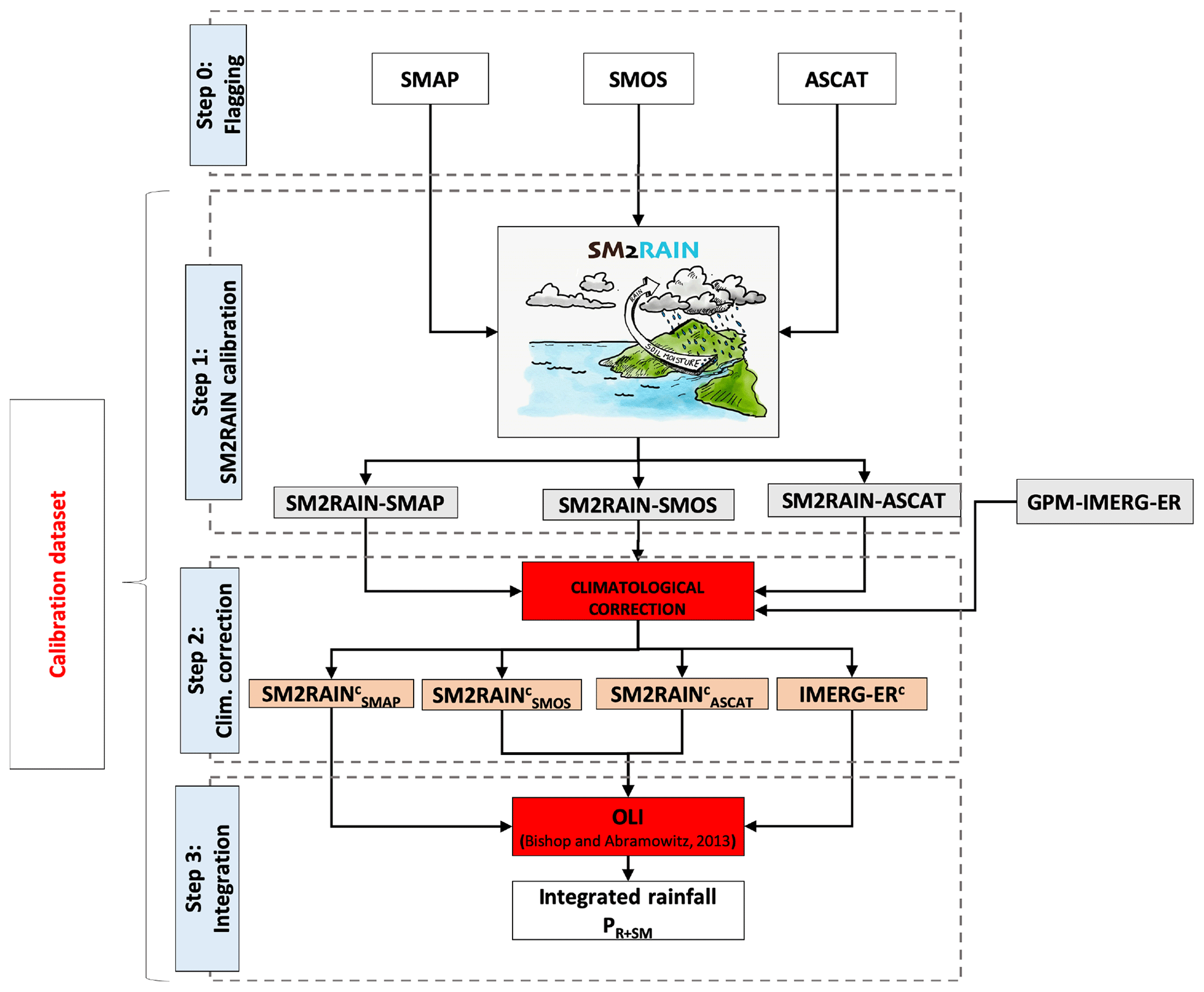
Figure 1Integration scheme used for the calculation of the integrated rainfall product PR+SM. In step 2, , , and IMERG-ERc refer to the SM2RAIN products with climatological correction (using the calibration dataset).
3.3.1 Step 0: soil moisture and rainfall pre-processing
Global SM and rainfall products come with different resolutions and grids. Moreover, the application of the SM2RAIN algorithm to SM observations requires preliminary processing. In step 0, we resampled all the datasets to the same grid over land between by using nearest-neighbour interpolation on the ASCAT grid (25 km). In particular, the IMERG products, characterized by a resolution of 0.1∘, were upscaled to 0.25∘ using a box-shaped kernel with antialiasing, an approach that was found to outperform simple spatial averaging. Rainfall accumulations were aggregated to daily scale (from 00:00 to 23:59 UTC).
As satellite SM data are not provided regularly spaced in time and contain gaps (for instance we did not include in the analysis observations characterized by frozen soils, snow presence or radio interference contamination; by using the specific flags for each product), they were linearly interpolated at 00:00 UTC to produce SM2RAIN daily rainfall from 00:00 to 23:59 UTC (see step 1). Note that we limited the interpolation to a maximum of 2 d; beyond that we assumed SM2RAIN rainfall were missing (in these cases only IMERG-ER is used in the integrated product as better described in Sect. 3.3.3). Note that the amount of missing data is generally dependent upon the location. Locations where the quality of satellite SM observations is poor are characterized by a lot of missing data, and the integrated product is basically close to IMERG-ER.
3.3.2 Steps 1 and 2: calibration phase
Step 1 refers to the calibration of SM2RAIN for the selection of the optimal parameters distribution pixel by pixel. All the parameters described in Sect. 3.1 were selected by using YREF. For that, we minimized the daily root mean squared error (RMSE) between the SM2RAIN rainfall applied to the specific SM product and YREF during 2015–2017. Note that as RMSE calibration is a variance-minimization technique, it is subjected to conditional biases, which can potentially determine a reduction of the temporal variability of the estimated precipitation and, thus, underestimate extreme values. To partially solve this issue, other metrics can be used, e.g. the Kling–Gupta efficiency (KGE) index (Gupta et al., 2009), which are theoretically superior in this respect. However, to ensure homogeneity among all the calibration steps (see OLC theory in Sect. 3.2), we chose to use RMSE, keeping in mind that the results obtained here could be further improved. The products so obtained are referred to as SM2RAIN-ASCAT if the satellite SM observations were derived from ASCAT, SM2RAIN-SMOS if derived from SMOS and SM2RAIN-SMAP if derived from SMAP. In addition to these products, we also produced SM2RAIN-ASMR2* and SM2RAIN-ASCAT*, by using satellite SM observations derived from AMSR2 and ASCAT with non-calibrated parameters; i.e. we used constant parameters globally derived from previous studies as in Massari et al. (2017a). Remember that these two last products were not used within OLC but will serve then only for validation purposes with TC.
As depicted in Sect. 3.2, the application of OLC requires unbiased ensemble members. This implies matching the long-term temporal mean of YREF with the ones of IMERG-ER, SM2RAIN-ASCAT, SM2RAIN-SMOS and SM2RAIN-SMAP by using a different (and temporally constant) multiplication factor for each member (i.e. a factor that multiplied by the mean of the member guarantees the matching with the mean of the calibration dataset). However, applying this procedure resulted in an overall reduction of the quality of the SM2RAIN members because a temporally constant multiplication factor deteriorated the quality of light rainfall (<5 mm d−1) with an increase of the false alarms (due to the noise contained in the satellite SM time series). To overcome this issue, we adopted a slightly different strategy which, despite not guaranteeing a perfect matching of the long temporal means and thus not being theoretically optimal, limited the problem of the increase of false alarms. In practice, for each member (i.e. SM2RAIN-ASCAT, SM2RAIN-SMOS, SM2RAIN-ASCAT, SM2RAIN-SMAP and IMERG-ER), we calculated the ratio between its mean monthly rainfall (i.e. mean of all the Januaries, mean of all the Februaries and so on) and the monthly mean of YREF (obtaining one multiplication factor per month per pixel for a total of 12 multiplication factors for each grid point). These factors were then used to multiply the daily rainfall observations of each member (relative to the desired month) to obtain a monthly based rescaled daily rainfall estimate.
This procedure is in principle a climatological correction rather than a bias correction because it uses the climatology of YREF as a reference. It guarantees a more consistent spatial pattern of rainfall among the members prior to the application of OLC, which helps also to avoid spatial inconsistencies when different combinations of members are used within the integrated product. Note that this operation does not constrain the variability of the precipitation from year to year to the one of YREF, as it only redistributes rainfall within the year and guarantees all the members to be realigned to the same climatology. Note also that a similar procedure is used for the production of IMERG-ER and IMERG-LR products (Huffman et al., 2018) and can be easily implemented for its use in near real time once the 12 factors for each member are known. From here onward we will refer to this procedure as a climatological correction.
3.3.3 Step 3: application of OLC
For the application of OLC (i.e. integration), we proceeded by considering these three methodological aspects:
-
First off, we performed a quality check, by comparing the correlation coefficient of each SM2RAIN product with the calibration dataset (YREF). When the correlation was found less than 0.4 (i.e. no correlation), the product was automatically excluded, and OLC was applied on the reminder of them. If all the SM2RAIN products correlation fall below this threshold (for example in dense forests or high mountainous regions), only IMERG-ER was retained. The value 0.4 was set to exclude the poor performance of SM2RAIN products at such thresholds, which could potentially impact the overall quality of the integrated product. To select this value, we performed ad hoc experiments (not shown) over CONUS, Australia, Europe and India and found 0.4 as a good compromise to exclude problematic areas like those impacted by high RFI (radio frequency interference) in the SMOS SM product. However, its overall impact on the final results was found to be very small and only limited to some specific regions (e.g. high RFI, dense forests and desert areas, which were already masked out by the validation mask).
-
The calculation of the OLC coefficients in Eq. (5) is not computationally demanding and uses the full calibration time series (2015–2017). In particular, Eq. (5) provides the specific coefficients to be used in Eq. (6) at each time step. If one of the SM2RAIN products is not available at a specific time step for the reasons described in step 0 (see Sect. 3.3.1), we linearly redistributed the coefficients to the products available at that time step so that their sum is one (to ensure unbiased estimates).
-
The application of OLC among the SM2RAIN products and IMERG-ER was carried only when IMERG-ER values are larger than zero, taking advantage of the enhanced rain–no-rain detection accuracy of IMERG that uses DPR (Gebregiorgis et al., 2018a), whereas when IMERG-ER was zero, this value was kept in the merged product. This tactic mitigates the degradation of rainfall estimates during low-rainfall time steps as demonstrated by Massari et al. (2019).
-
The final product is then composed of multiple rainfall datasets weighed according to Eq. (6). IMERG-ER is always present, whereas the presence of the three SM2RAIN rainfall estimates derived from ASCAT, SMOS and SMAP depends on their relative accuracy (if they satisfy the threshold) and availability in time and space.
The success of the overall procedure described above is dependent upon the quality of YREF. Although the calibration phase seems very intensive, it will be demonstrated in Sect. 4 that if YREF has a relatively good accuracy, its effect on the final quality of the integrated product is very low. However, its choice is strategic in some regions, as will be shown in Sect. 4.1, and thus deserves a careful investigation.
3.4 Validation strategies
For the validation of the integrated product, two different strategies were followed. First, we selected four key regions characterized by different climates and landscapes (i.e. CONUS, AU, EU and IN) where ground-based observations (derived from rain gauges and rain gauges plus radar) are very dense and of a high quality (see Sect. 2.1). Both continuous and categorical scores are considered, as commonly used in a classical validation of global precipitation products (see Maggioni et al., 2016, for further details).
Next, since many areas of the world like Africa, South America and central Asia have a highly variable density of rain gauges, validation was also performed using a TC analysis as proposed by (Massari et al., 2017a; Khan and Maggioni, 2019; see Sect. 3.4.2). TC offers a viable way to validate rainfall products in data-scarce regions by providing (theoretical) error and correlation of each product with the “unknown” truth. Note that we tested the validity of the TC validation by applying it to the same key regions where the classical validation was carried out. Then, TC was applied to Africa and South America to validate the integrated product and the other datasets that are part of the analysis. The validation with TC was carried out in 2018 (only 1 year), which is independent from the calibration period (2015–2017).
3.4.1 Classical validation
Both continuous and categorical error metrics were adopted for validating daily rainfall. The continuous scores are the following:
-
Pearson correlation coefficient (R).
-
Root mean squared error (RMSE).
-
Additive bias (BIAS).
-
Variability ratio (γ). This is where γ is the ratio of the standard deviation of the rainfall estimate σs and the one of the benchmark σo. The optimal value of γ is 1.
-
Kling–Gupta efficiency index. KGE is a modified version of the classical Nash–Sutcliffe (NS) efficiency index commonly used for evaluating discharge simulation estimates. KGE is composed of three terms: correlation, variability ratio and bias. KGE varies from −∞ to 1. KGE values close to 1 denote perfect model estimates, whereas values of KGE indicate that the estimate deteriorates upon the mean rainfall benchmark (Knoben et al., 2019). With respect to NS, KGE gives more weight to the variability component and is less impacted by conditional bias. In this study, we used the version of KGE proposed by Beck et al. (2019). For further details on the topic, we refer the reader to Gupta et al. (2009).
In addition, three categorical scores were considered: the probability of detection POD=H ∕ (H+M), which measures the likelihood of the rainfall estimate to detect an event when it in fact occurs; the false alarm ratio FAR ), which measures the likelihood that a precipitation event does occur when a reference does not estimate rain; and the threat score (TS), which is an integrated measure of POD and FAR. All these scores are based on the contingency table (Table 1). In the table, H represents hit cases when both the precipitation estimate and reference are greater than or equal to the rain–no-rain threshold percentile (th); F represents false alarms, when the precipitation estimate is greater than or equal to th but when the reference is less than th; M represents missed events, when the reference is greater than or equal to th but when the precipitation estimate is less than th; and Z represents correct no-rain detection, when both the precipitation estimate and reference are less than th. N is the sample size, i.e. the total number of observed events and .
Table 1Contingency table commonly used for characterizing detection errors of precipitation products.

3.4.2 Triple-collocation analysis applied to rainfall observations
In this study, TC analysis (Stoffelen, 1998) was applied to estimate the correlation and the error of the rainfall estimates when a reliable reference is missing like in Africa. Here we present a summary of the theory behind TC, while the reader interested in more details can refer to Massari et al. (2017a).
Suppose we have three measurement systems Xi, observing the true variable t characterized by an additive error model
where the variables Xi (i=1, 2, 3) are collocated measurement systems linearly related to the true underlying value t with additive random errors εi, respectively, while αi and βi are the ordinary least-squares intercepts and slopes. Assuming that the errors from the independent sources have zero mean (E(εi)=0) and are uncorrelated with each other (Cov(εi,εj) =0, with i≠j) and with t (Cov(εi,t) =0), the variance of the error of each dataset can be expressed as (McColl et al., 2014)
where is the covariance within the variables Xi.
In addition, McColl et al. (2014), using the definition of the correlation and covariance, demonstrated that
where is the squared correlation coefficient between t and Xi (McColl et al., 2014).
Note that the error (and correlation) calculated via TC is generally lower (higher) than those calculated using the classical validation, given that it does not include the reference uncertainty.
3.4.3 Validation mask
Although the integrated product is potentially available everywhere, we found that where the quality of satellite SM observations is very low like in forests, frozen soils and mountainous areas, OLC coefficients associated with the SM2RAIN products were very small, and the integrated product was mainly constituted by IMERG-ER. Therefore, to avoid any misinterpretation about the real benefit of integrating IMERG-ER with satellite SM observations, we limited the validation of the integrated product to the ASCAT committed area (Hahn, 2016). The area is limited to low and moderate vegetation regimes, unfrozen and no snow cover, low to moderate topographic variations, no wetlands, no coastal areas, and no deserts (see Fig. S3 of the Supplement). Outside of this area, satellite SM observations might suffer from several problems and are weighed much less by OLC (although we also found benefits here; see Sect. 4.1.1). In addition, for the sake of product distribution and use, we can ensure optimal results only over this area, and thus we associated a flag to the pixels which fell outside it in the netCDF file included in the Supplement.
Both the calibration of SM2RAIN and the OLC implementation need a calibration dataset as described in Sect. 3.3 (i.e. YREF). The choice of this dataset is strategic for obtaining a good-quality integrated product. Section 4.1 describes the process of the selection of YREF considering different potential candidates. Section 4.1.1 and 4.1.2 describe the validation over US, IN, AU and EU by using the hydrometeorological networks described in Sect. 2.1 and the validation in Africa and South America by using TC (Sect. 3.4.2), respectively.
4.1 Calibration dataset selection
The choice of a calibration dataset is strategic for both the SM2RAIN parameters selection and the OLC coefficients calculation. Thus, it has to be carefully selected based on (i) accuracy (i.e. low error and high correlation with “true” rainfall), (ii) homogeneous performance in time and space, and (iii) continuous spatial and temporal coverage (as well as spatial and temporal resolution closer to the one of the rainfall to be estimated). Potential candidates are:
-
GPCC. This has potentially high accuracy and low biases where the rain gauge coverage is good but can be unreliable when the rain gauge distribution is scarce (e.g. Africa and South America). It might also suffer from time dependence performance as a function of rain gauge availability.
-
ERA5. This provides full coverage and generally homogeneous performance all over the world.
-
IMERG-FR. This is a gauge-corrected satellite product and potentially highly accurate where rain gauges distribution is dense. The drawback is that it is highly dependent upon IMERG-ER where rain gauge observations are scarce. For this reason, we initially excluded this product from the list of potential candidates and focused only on the other two.
To explore the performance of ERA5 and GPCC, we applied TC as described in Sect. 3.4.2 during the whole period 2015–2018. The following triplets were used (by keeping in mind the need to satisfy the assumptions of TC highlighted above):
-
GPCC, IMERG-ER and SM2RAIN-ASCAT* (triplet A)
-
GPCC, IMERG-ER and ERA5 (triplet B)
-
GPCC, ERA5 and SM2RAIN-ASCAT* (triplet C).
Note that SM2RAIN-ASCAT* above is not the one used in the integration, but it was produced using constant parameters a, b and Z all over the world (i.e. it is not regionally calibrated) as in Massari et al. (2017a) to avoid a potential violation of the TC assumptions. On the other hand, even using SM2RAIN-ASCAT (the calibrated dataset), similar results were obtained (not shown), as we found a negligible effect of the calibration on TC results (in terms of TC correlations).
Table 2 shows results for triplet A, B and C. Different configurations of the triplets provide similar results, suggesting that TC can be considered reliable. In particular, ERA5 performs the best among all, but it also suffers from significant uncertainty over convection-dominated systems like in western Africa and the Sahel (see Fig. 2). Elsewhere, the performance is relatively good except over north-western CONUS and tropical forests of Africa and Indonesia. The GPCC product provides relatively good performance over Europe, eastern Asia, Australia and Canada, but its performance are very low over Africa.
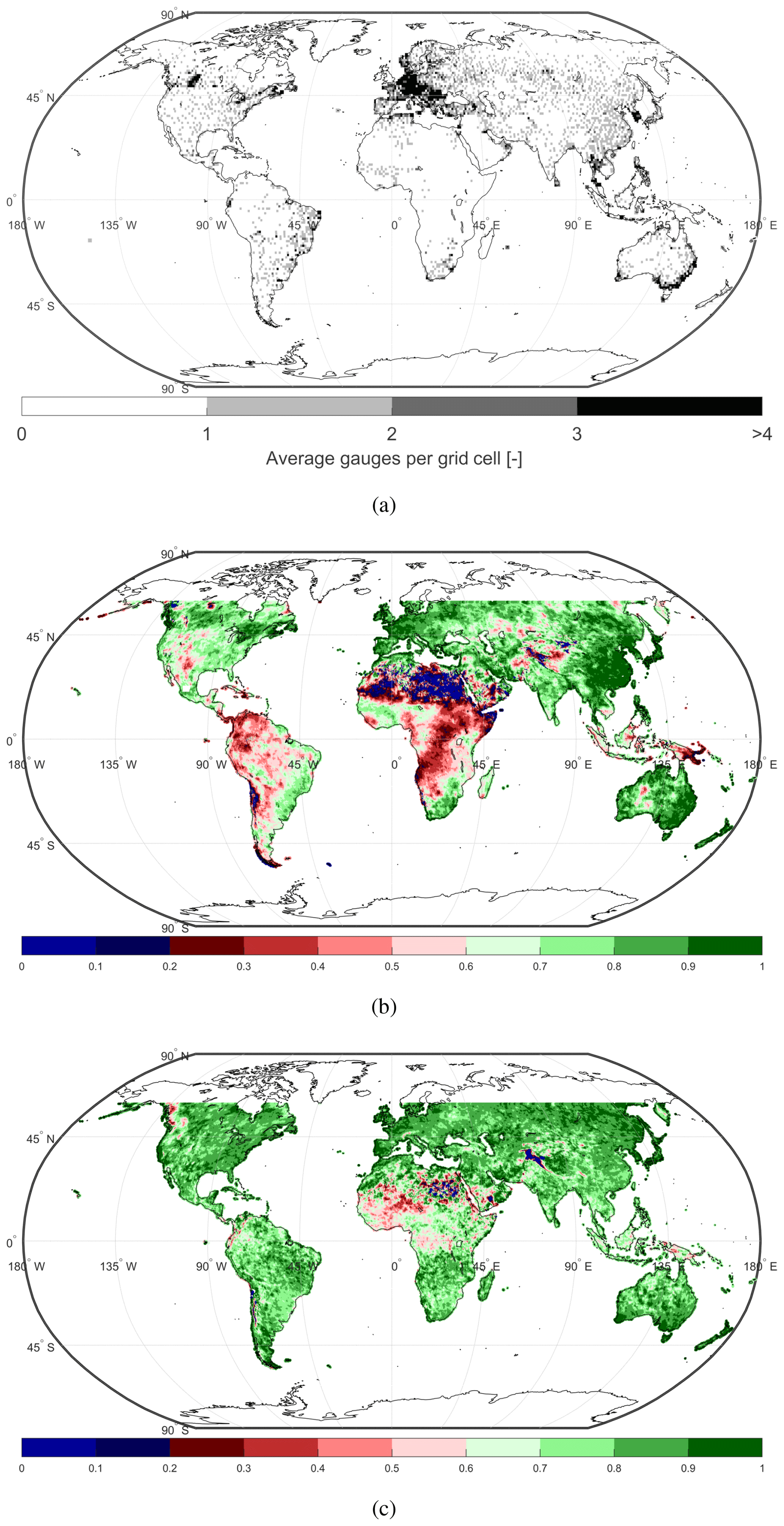
Figure 2(a) Number of stations used for the GPCC First Guess 1.0∘ product for the years 2015–2018. (b) TC correlation of the GPCC First Guess 1.0∘ product in Africa during 2015–2018 using the triplet GPCC, ERA5 and SM2RAIN-ASCAT*. It can be seen that lower correlation areas closely match with areas of low station density. (c) TC correlation of the ERA5 reanalysis during 2015–2018 for GPCC, ERA5 and SM2RAIN-ASCAT*.
Table 2Triple-collocation correlation obtained by using triplet (A) GPCC–IMERG-ER–SM2RAIN-ASCAT, (B) GPCC–IMERG-ER–ERA5, (C) GPCC–ERA5–SM2RAIN-ASCAT for the period 2015–2018. The numbers refer to median values.
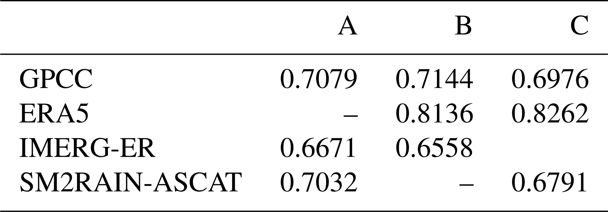
Figure 2a plots the number of stations used for the GPCC First Guess 1.0∘ product for the years 2015–2018, whereas Fig. 2b and c show the TC temporal correlation of the GPCC and one of ERA5 for the period 2015–2018. An interesting feature is that lower correlations of GPCC closely match with areas of low station density (by comparing Fig. 2a and b), whereas ERA5 shows a more homogeneous and higher correlation over all the globe. It has also to be noted that the number of stations used by GPCC in Africa during this period is very low with areas totally uncovered, which likely leads to significant interpolation error. The uneven rain gauge spatial distribution seems to significantly impact the GPCC quality and in turn can potentially cause sub-optimal performance if used as a calibration dataset. ERA5 relies less on observation density and shows a more homogeneous performance pattern with respect to GPCC. Thus, ERA5 was selected as YREF. This selection does not guarantee optimal solutions, but it is the best we can do with the available datasets considering that other potential candidates can be affected from other or similar issues, which could result in a very different global precipitation estimate (Herold et al., 2016). The solution to this problem is not straightforward, but a possible way forward would be the integration of GPCC and ERA5 or the use of available integrated products (Beck et al., 2017). The advantage of relying only on a single rainfall source (as to ensure homogeneity) however will be lost in that case.
Note that, except for CONUS where rain gauge information is ingested into ERA5 (Lopez, 2011), the integrated product is totally independent of the rain gauge. This allows for independently cross-validating the integrated product in EU, IN, AU and CONUS during 2015–2017 against high-quality ground-based rainfall observations (see Sect. 4.1.1). The latter serves to understand if the entire procedure of integration described in Sect. 3.3 is correct and provide an overall idea of the maximum potential performance that can be obtained by the integrated product (being performed in the same period used for calibration).
4.1.1 Classical validation over key regions using high-quality ground-based observations
Figure 3 summarizes the products used in PR+SM pixel by pixel for the different key regions. While for India and Australia, SM2RAIN-ASCAT, SM2RAIN-SMOS and SM2RAIN-SMAP are present almost everywhere, over CONUS and Europe there exist areas where SM2RAIN-SMOS was not used either because radio frequency interference which was too high was found in the SMOS product or because of its relatively low performance (Chen et al., 2018). In the figure, we did not superimpose the mask described in Sect. 3.4.3 to show that the areas in dark blue (i.e. where only IMERG-ER is retained) almost coincide with the ASCAT-committed area. For instance the north-eastern CONUS region is known to be a challenging area for satellite SM products, and, as a result, here PR+SM relies on IMERG-ER alone. Similarly, the coastal areas are mostly characterized by dark-blue pixels, which indicates no integration with any SM2RAIN product. Note however that the ASCAT committed area does not always match the area where only IMERG-ER is present, e.g. north-eastern Africa. Here, the ASCAT SM product is known to perform relatively poorly due to volume scattering (Wagner et al., 2013), whereas passive products perform relatively well (in orange, the presence of only passive sensors integrated with IMERG-ER can be seen). Although in areas like this we still have an improvement of IMERG-ER, they could be considered part of the integrated product we preferred to be conservative and guarantee the product reliability only over the mask described in Sect. 3.4.3.
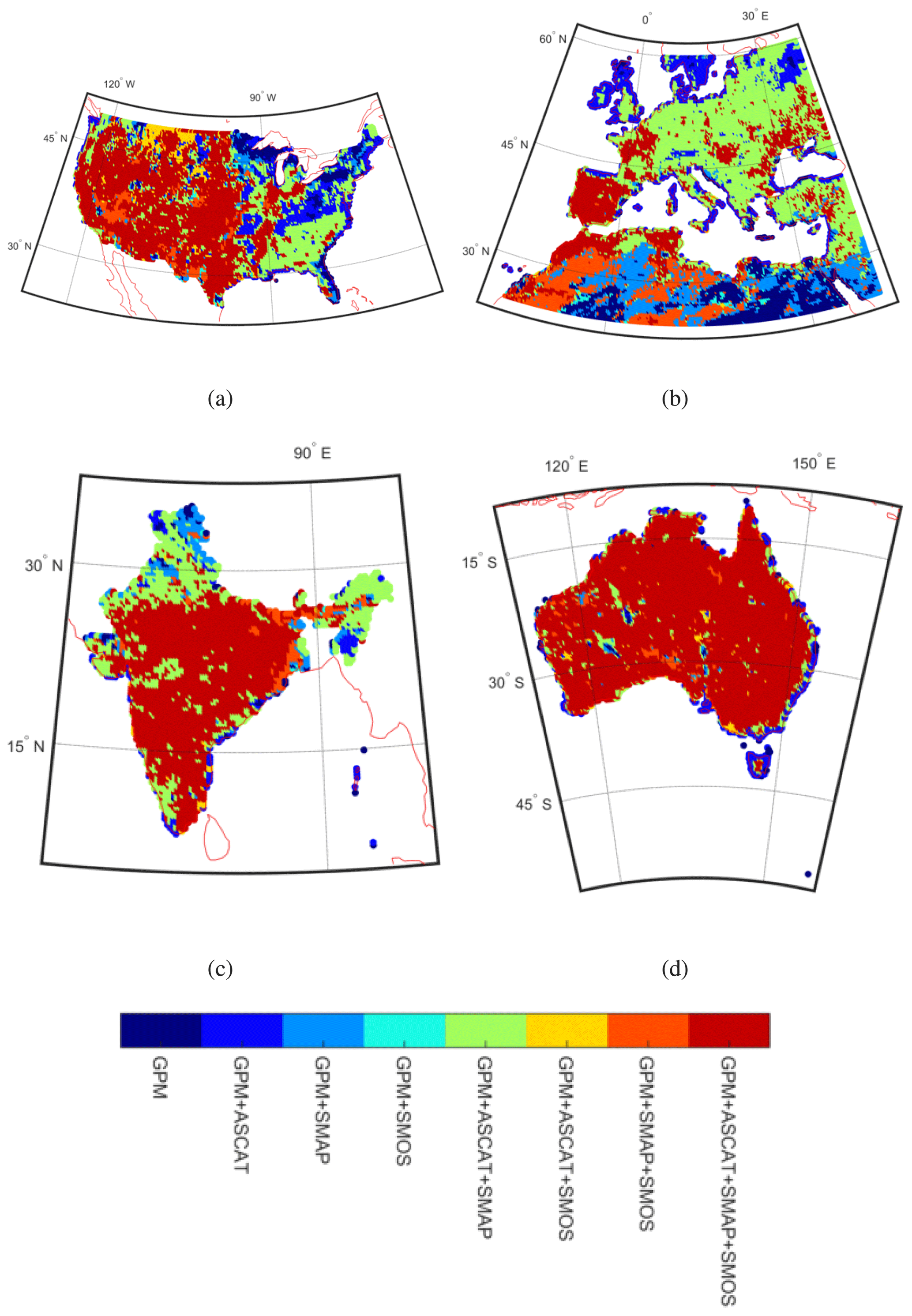
Figure 3Products used in the integration over CONUS (a), Europe (b), India (c) and Australia (d). The results refer to 2015–2017 period.
Table 3 shows R, RMSE, BIAS and KGE of the different rainfall products obtained by using the ground-based observations described in Sect. 2.1 as references. The short-latency products (less than 2–3 d) are shown in light blue, whereas the long-latency ones (larger than 2 months) are left white. The integrated product PR+SM outperforms both IMERG-ER (significantly) and in some cases long-latency products in terms of R and RMSE (see for instance PR+SM correlations in Australia, Europe and India vs. ERA5 correlations). This suggests that the selection of the calibration dataset is not necessarily a major limiting factor in the proposed framework, as satellite SM contains inherent information about rainfall, as long as its quality is sufficiently high. However, this is not always true for all the scores. For instance, in terms of bias, results are not optimal in India. Here, ERA5-based climatological correction is probably the reason for the sub-optimal performance of the integrated product due to the relatively high bias of ERA5 over India. For other regions, results are overall good in terms of bias for PR+SM, although they are slightly worse for CONUS. The bias for IMERG-ER is particularly relevant over CONUS and Europe, as well as for IMERG-FR in Europe. On the other hand, GPCC and ERA5 biases over these regions and in Australia are very low, which is expected due to the large amount of gauge stations shared with the references.
Table 3Median correlation (R), root mean square error (RMSE), daily bias (BIAS), variability ratio γ (i.e. ratio between the standard deviation of the estimated rainfall and that of the benchmark) and the Kling–Gupta efficiency (KGE) index obtained with the comparison of the different rainfall products against gauge-based AWAP (Australia), Stage IV (CONUS; gauge and radar), E-OBS (Europe) and IMD (India) during the period 2015–2017. PR+SM refers to the integrated product. Asterisks refer to short-latency products, while values in bold denote the best performing product in the region according to the specific score on the left.
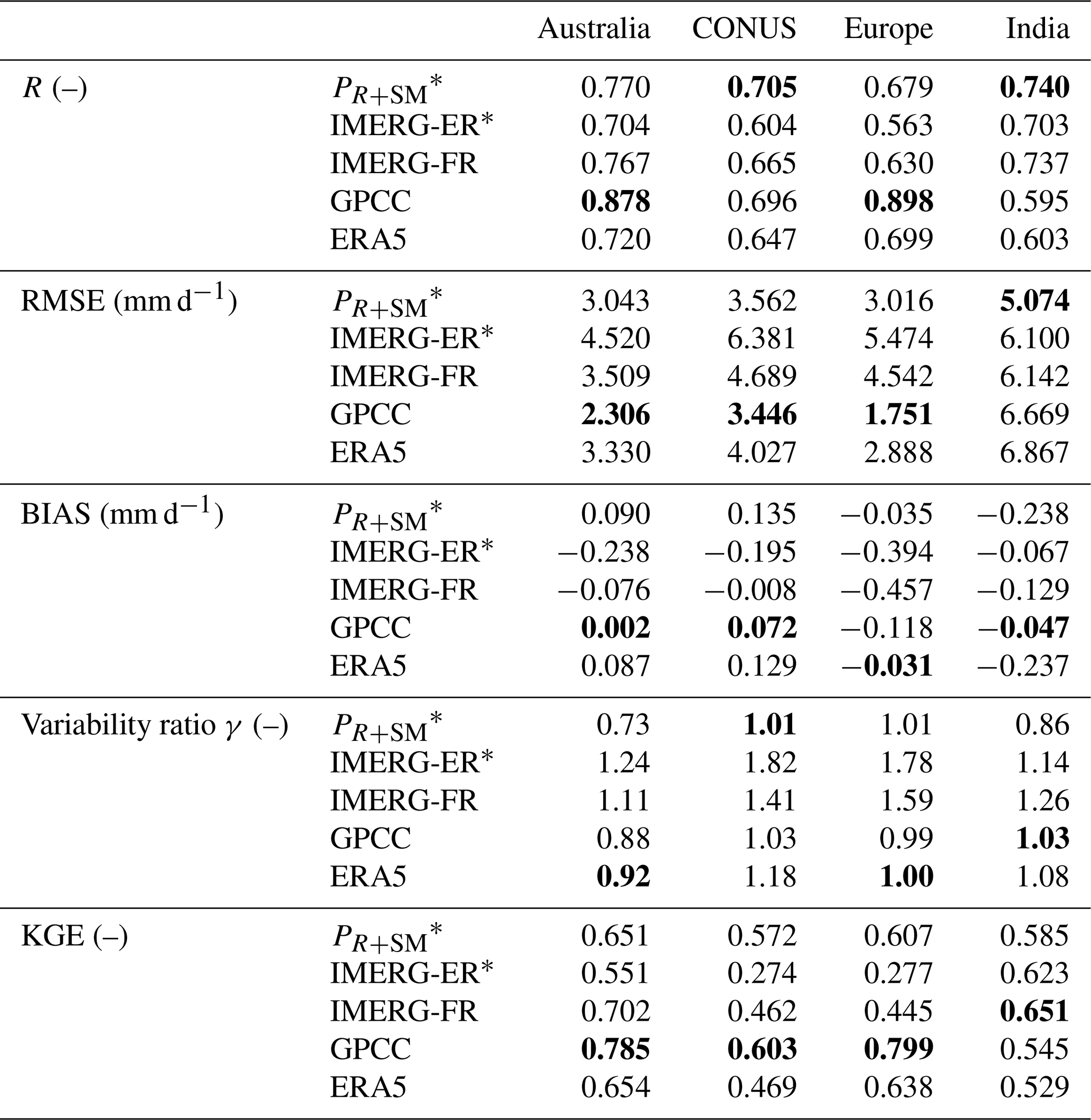
In terms of the variability ratio, we did not observe significant conditional biases of the PR+SM product in Europe and CONUS, although the use of RMSE as a calibration score of SM2RAIN (see Sect. 3.3.2) and in the OLC procedure (see Sect. 3.2) would systematically suggest it. Rather, we observed the ability to reduce the high variability of IMERG-ER bringing it to values closer to one. Only for Australia is γ about 30 % lower than one, but this difference is not too far from the range of values observed for the other products (especially GPM-based products). The reason for that can be twofold. First, the integration was carried out only on non-zero rainfall values (thus the impact of SM2RAIN calibration with RMSE is overall lower than expected; see Sect. 3.3.2). Second, the lower variability of SM2RAIN products is in this case beneficial as IMERG-ER shows variability which is too high.
KGE results provide an integrated measure of the scores discussed above. PR+SM KGE values range around 0.6 for all the key regions. Lower performance is obtained for IMERG-ER with respect to PR+SM due to its high variability, except for India where the higher bias of PR+SM determines sub-optimal KGE. For long-latency products, KGE measures are relatively good for GPCC, except in India where its lower correlation determines a decrease of KGE. IMERG-FR suffers from a large variability ratio in Europe (in addition to high bias) and CONUS, which causes relatively low KGE values. ERA5 KGE values are sub-optimal over CONUS (due to a high bias and low variability ratio) and in India (due to high bias).
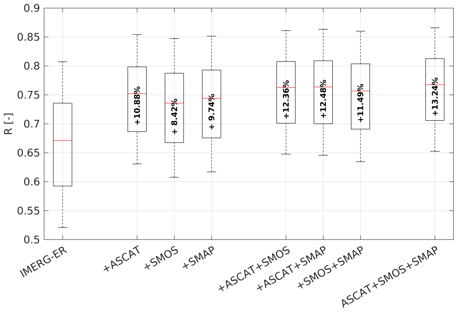
Figure 4Correlation increments obtained by ingesting ASCAT, SMOS and SMAP SM2RAIN-based rainfall estimates into the IMERG-ER product. Values in bold inside the box plots refer to the median increments expressed in terms of percentage. The box plot refer to the 25th and 75th percentiles, while the whiskers refer to the minimum and maximum values. Outliers are not shown in the plot.
Figure 4 shows, for AU, the increase in temporal correlation (2015–2017) with respect to IMERG-ER obtained by integrating the latter with one (either ASCAT or SMAP or SMOS), two (either ASCAT+SMOS, SMAP+SMOS or ASCAT+SMAP) or three SM2RAIN products (ASCAT+SMAP+SMOS). The addition of multiple products, though beneficial, gets smaller as we ingest more SM2RAIN-based rainfall estimates. This is due to the redundancy of information provided by SM, which causes no further improvement. Although this might suggest that using a single SM2RAIN product is equivalent to using multiple products, the use of multiple products always guarantees optimal performance per pixel and is useful where one of the products does not perform well, as shown in Fig. 3. Results for the other key regions provide similar overall conclusions and are not shown here.
Figure 5 shows the correlation and RMSE differences in percentage obtained between the integrated product and IMERG-ER. Blue areas are those characterized by improvements, whereas red denotes deterioration. There is an overall improvement for both scores over the study areas. Larger improvements are obtained in terms of RMSE, which in some cases (i.e. CONUS) are larger than 40 %. In terms of R, the improvement spans from 5 % to 15 % with larger values obtained for Europe and Australia. There are also spots over north-western CONUS characterized by deterioration. We attributed this to the low agreement between stage IV data and ERA5 data (used as calibration dataset), which can be also found in Beck et al. (2019). Note this is a challenging area for Stage IV data, as also demonstrated by Tian et al. (2007), who found significant performance differences of the Tropical Rainfall Measuring Mission (TRMM) 3B42 rainfall product in north-western CONUS when compared either to the CPC (Climate Prediction Center) Unified Gauge-based Analysis of Global Daily Precipitation (Higgins et al., 2000) product or with the Stage IV dataset.
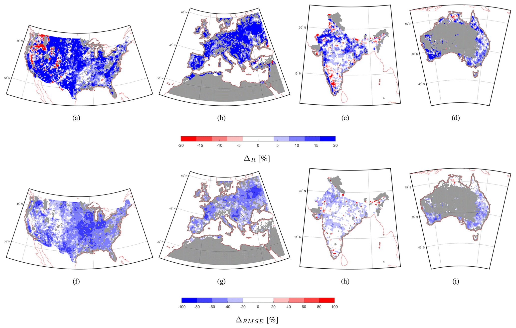
Figure 5Percentage differences in correlation (ΔR in percentage; panels a, b, c, d) and in root mean square error (ΔRMSE in percentage; panels f, g, h, i) between the integrated product PR+SM and the IMERG Early Run (IMERG-ER) product over CONUS, Europe, India and Australia for the period 2015–2017. Grey areas represent the masked areas based on what is described in Sect. 3.4.3.
To understand the benefit of integrating SM-based rainfall with IMERG-ER as a function of the topographic complexity, Fig. 6 shows the median differences, in terms of correlation (panel a) and RMSE (panel c), obtained by PR+SM with respect to IMERG-ER for CONUS. The topographic complexity comes along with the ASCAT H115 product and is computed as the normalized standard deviation of elevation using GTOPO30 data (Hahn, 2016). It ranges between 0 % for flat areas and 100 % for very complex terrain. The integrated product is able to improve the quality of IMERG-ER over flat areas better than complex terrain. This result is somehow expected, as we know that the topographic complexity impacts the quality of the SM retrieval.
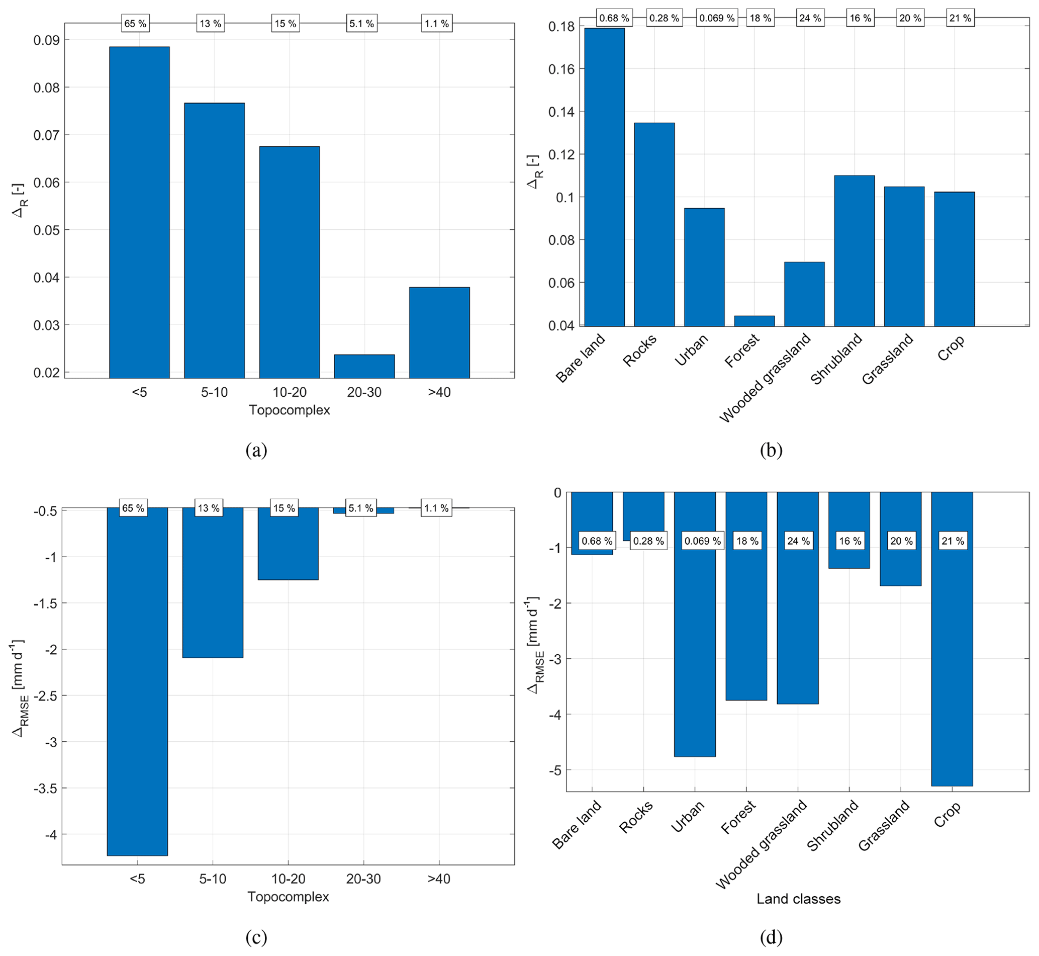
Figure 6Difference in median correlation (ΔR) and in median root mean square error (ΔRMSE) between the integrated product PR+SM and IMERG-ER as a function of the topographic complexity (a, c) and as a function of the land cover type (b, d) over CONUS. The results refer to the 2015–2017 period. The text boxes on the top show the percentage of the area occupied by the specific topographic complexity or land cover type.
The benefit of the integration was also computed as a function of land cover (panels b and d in Fig. 6 for CONUS). Land cover information comes from the ECOCLIMAP dataset (a global database of land-surface parameters at 1 km resolution Champeaux et al., 2005), provided at 1 km spatial resolution. We have simplified the original land use classes into eight categories: bare land, rocks, urban, forest, wooded grassland, shrubland, grassland and crop. Except for urban, rock and bare soil (with a percentage of pixels within CONUS of less than 0.5 %), the integrated product performs better over shrubland, grassland and crop, whereas lower performance is obtained over forests. This result is also expected as the quality of the satellite SM product can be highly impacted by the presence of dense vegetation for the difficulty of the retrieval in separating the effect of the soil water content from the water contained in leaves.
Figure 6 refers to CONUS, as we found highly representative of different landscape complexity and land cover type. Results for AU, EU and IN show very similar findings and are reported in the Supplement (Figs. S4 and S5).
Figure 7 shows the differences in terms of POD, FAR and TS between the integrated product PR+SM and IMERG-ER as a function of the rainfall percentiles. As the correction of IMERG-ER was only carried out for positive rainfall values and SM2RAIN-based rainfall lower than 1 mm was assumed unreliable (to exclude the possibility of interpreting satellite SM noise as rainfall; Zhan et al., 2015), the differences with respect to IMERG-ER are visible only above the 50–60th percentiles.
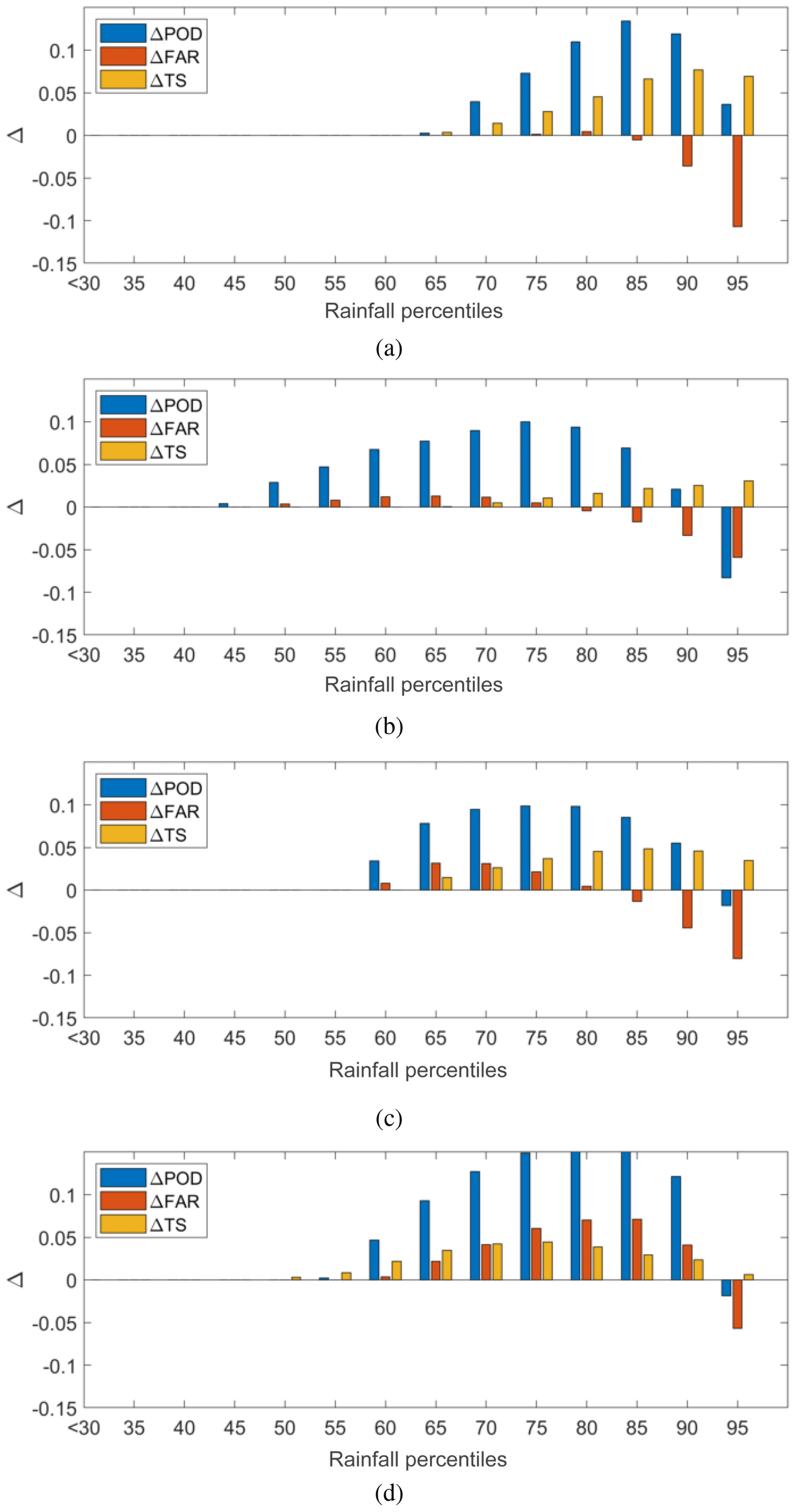
Figure 7Difference in categorical indices (probability of detection – POD, false alarm ratio – FAR – and threat score – TS) between the integrated product PR+SM and the IMERG-ER as a function of the rainfall classes for Australia (a), CONUS (b), Europe (c) and India (d) for the period 2015–2017. The bars refer to median values.
After the 50–60th percentiles, a significant increment of POD is evident for all the study regions, whereas the differences in FAR denote a deterioration from the 50th to 80th percentile across CONUS, EU and AU (very small) and in IN (much larger). The latter seems caused by more noisy satellite SM observations over India, which directly impacts the quality of SM2RAIN estimates (causing higher FAR; see also Zhan et al., 2015 and Massari et al., 2019). This problem could be faced by de-noising satellite SM observations with methods similar to the ones proposed by Massari et al. (2017b) and Su et al. (2014, 2015) or by selecting a higher rainfall threshold below which only IMERG-ER is retained (i.e. larger than 1 mm selected above). The improvement in terms of FAR becomes significant for higher rainfall accumulations (i.e. 95th percentile). The overall improvement is shown by the TS score, which is generally positive, suggesting that the integrated product helps to improve IMERG-ER in terms of categorical scores especially for the 70–90th percentiles.
4.1.2 Validation over data-scarce regions using TC
Prior to the assessment of the rainfall products over Africa and South America with TC, we run TC analysis over AU, CONUS, EU and IN, where R and RMSE scores obtained with the classical validation are available. Results are described in Supplement Sect. S1 and show that TC provides similar conclusions to a classical validation and can therefore be used as a robust validation tool over data-scarce regions.
Figure 8 shows the product combinations for each pixel of the study areas used for obtaining PR+SM in Africa and South America. These combinations and the associated OLC coefficients (including the SM2RAIN parameter calibration) were obtained during the calibration period 2015–2017. Areas where all SM2RAIN products are ingested match with those characterized by a relatively good quality of satellite SM observations, i.e. those not characterized by dense forests, desert areas and frozen soil, as well as snow-covered areas. This suggests that the integration is robust and meaningfully excludes low-quality SM information.
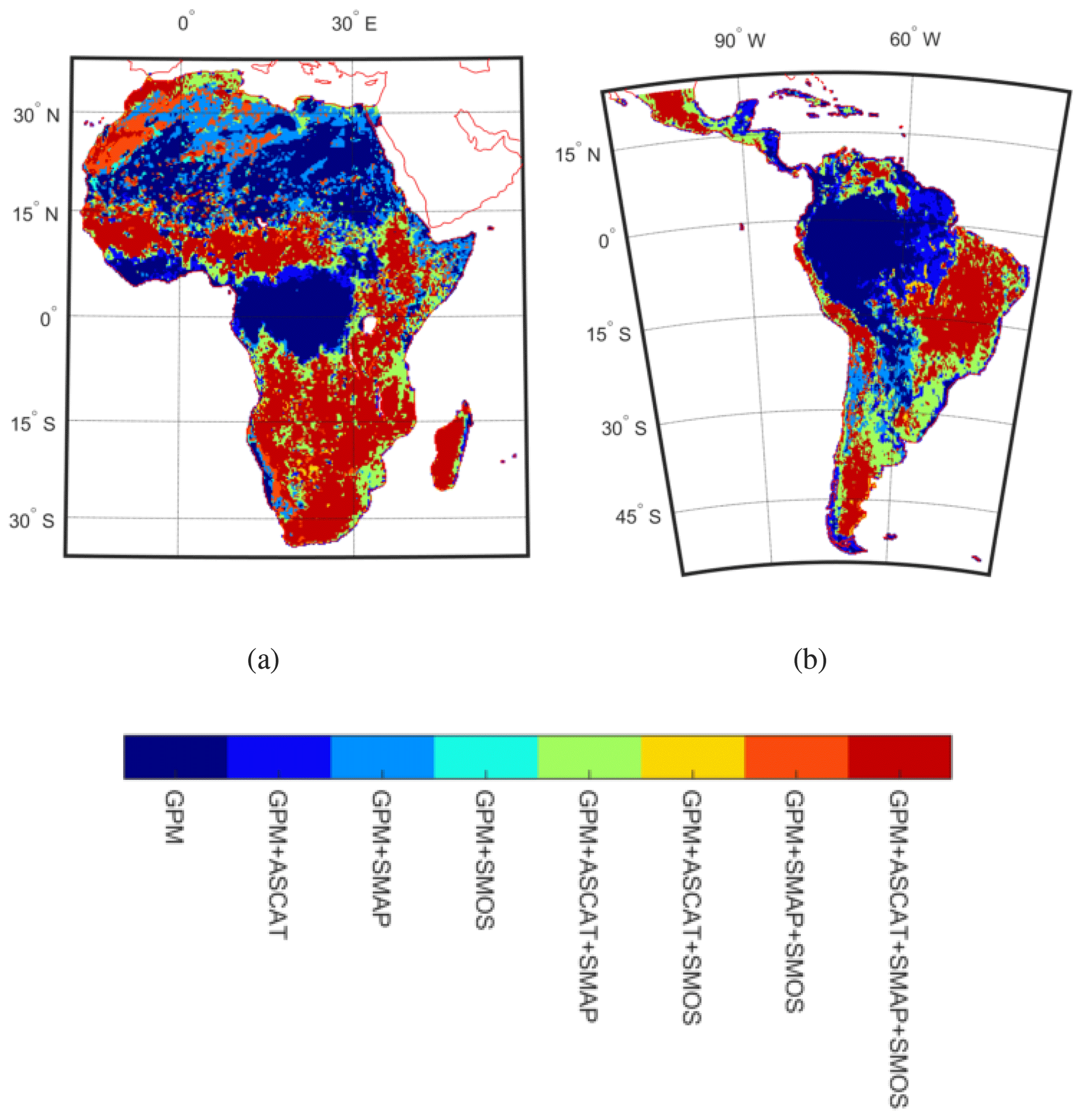
Figure 8Products used to integrate IMERG-ER with SM2RAIN products derived from the setup during the calibration period in South America. When low correlation was found between the reference dataset (i.e. GPCC) and the SM2RAIN product, the latter was excluded from the analysis, and only IMERG-ER was retained.
Unlike the results presented in Sect. 4.1.1, here we validate the products during 2018, independent from the calibration period (i.e. 2015–2017). As in Africa and South America, the rain gauge distribution is scarce (see Fig. 2a), with the validation being carried out via TC, using three triplets built among ERA5, SM2RAIN-ASCAT*, PR+SM, GPCC and IMERG-ER:
-
ERA5–GPCC–IMERG-ER
-
ERA5–GPCC–SM2RAIN-ASCAT*
-
ERA5–GPCC–PR+SM
Figure 9 shows (left) and TC-RMSE (right) over Africa obtained by triplets 1 (ERA5–GPCC–IMERG-ER) and 3 (ERA5–GPCC–PR+SM). In particular, panels a-d refer to the short-latency products, while the rest of them are long-latency ones (>2 months). The integrated product outperforms both IMERG-ER and long-latency products like GPCC and ERA5, as we found in Sect. 4.1.1. ERA5 is characterized by lower performance in the Sahel region as highlighted in Fig. 2b, whereas GPCC is strongly affected by the uneven rain gauge distribution, as depicted in Fig. 2c. Similar results are obtained for South America in Fig. 10, where the central eastern part gets greener (higher correlation) and whiter (lower error) after integration with SM2RAIN-based rainfall estimates. In South America the performance of ERA5 is higher than the one obtained in Africa and consistently more homogeneous.
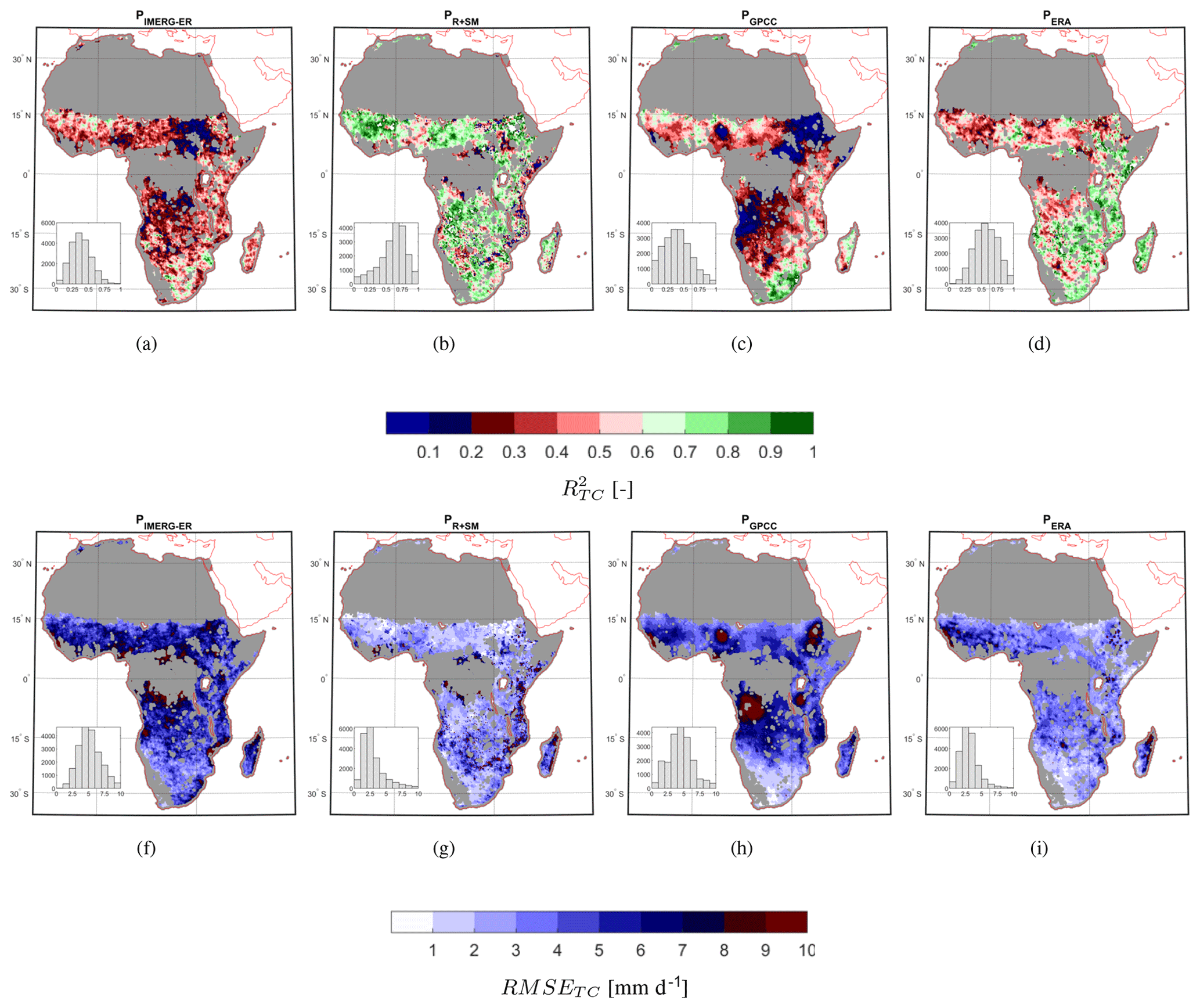
Figure 9Triple-collocation squared correlation (; panels a, d) and root mean square error (RMSETC; panels f, i) in millimetres per day for IMERG Early Run (IMERG-ER; panels a and f), the integrated product (IMERG Early Run and SM2RAIN applied to ASCAT, SMAP and SMOS; PR+SM; panels b, g), the Global Precipitation Climatology Center product (GPCC; c, h) and the reanalysis product ERA5 (ERA5, d, i). Grey areas represent the committed area of ASCAT which we excluded from the analysis. The results refer to the validation period (i.e. 2018). Grey areas represent the masked areas based on what is described in Sect. 3.4.3.
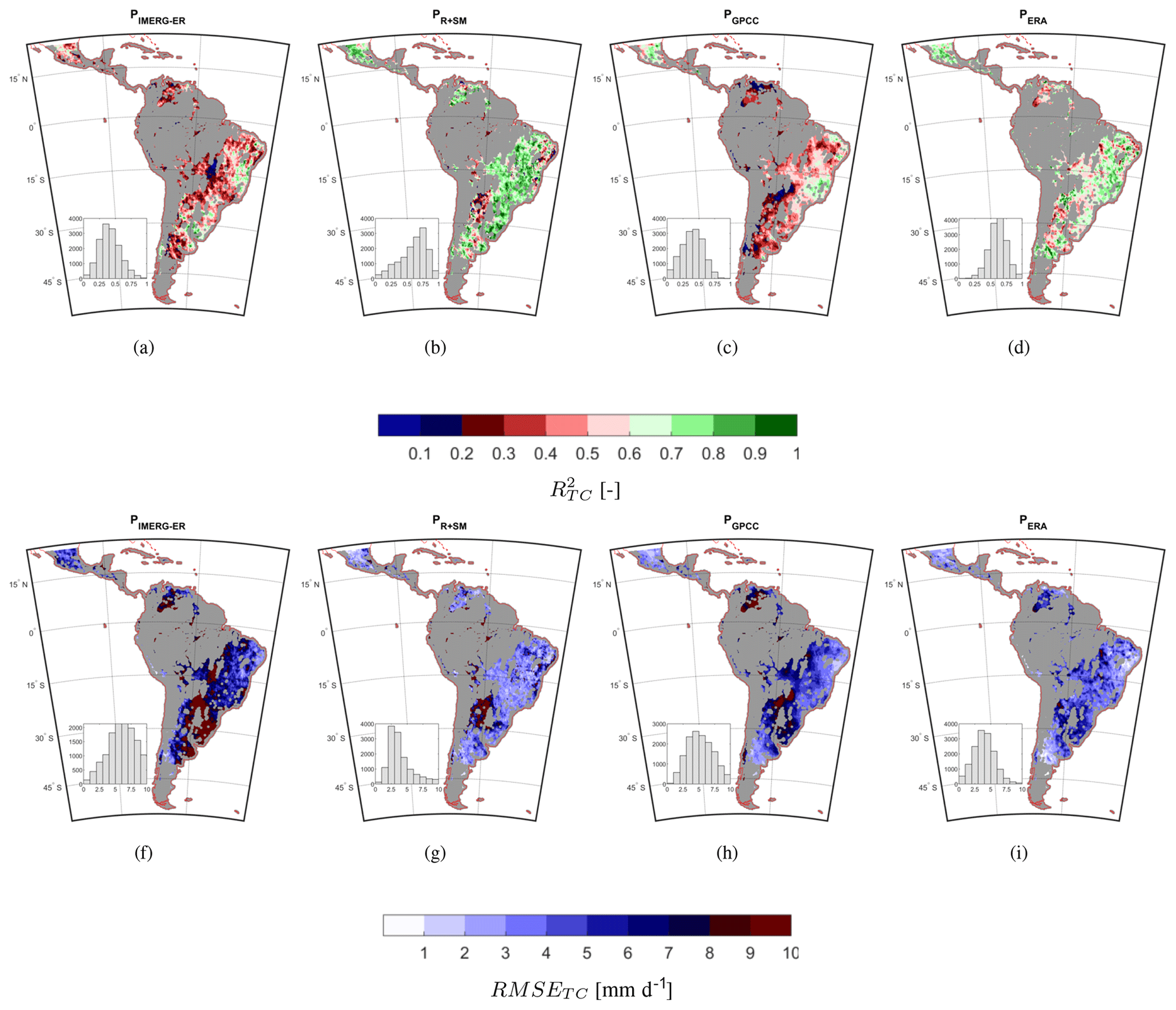
Figure 10As in Fig. 9 but for South America.
Figure 11 summarizes the results obtained in the two regions by considering only the committed area (panels a and b) and all the pixels of the analysis (non-masked by the committed area; panels c and d) also in terms of boxplots. It can be seen that in Africa (panels a and c) the integrated product is always the best both in terms of error and correlation. In South America (panels b and d), ERA5 outperforms the integrated product if no mask is used (panel d). A reason for that is the lower skill of IMERG-ER over dense forests especially in terms of error, which impacts the overall quality of the integrated product. In particular, relatively good performance is obtained in Africa over the Sahel region and in South America over eastern Brazil.
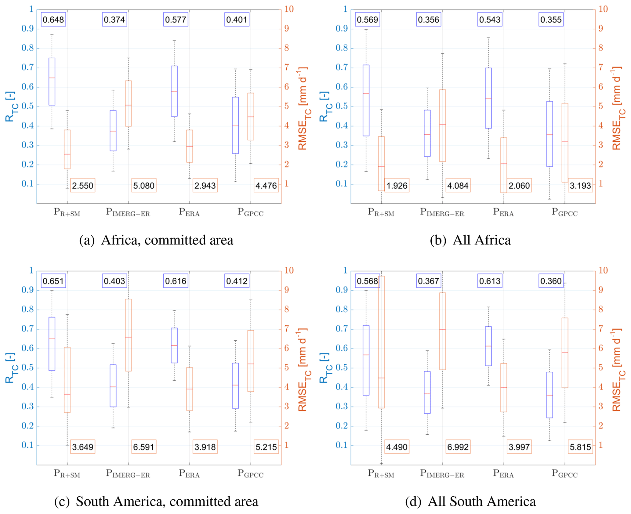
Figure 11Box plots of triple-collocation squared correlation (; left axis in blue) and root mean square error (RMSETC; right axis in red) in millimetres per day obtained during validation period (i.e. 2018) in Africa over the committed area mask (a) and over the whole study area (b). Panels (c) and (d) refer to the same results but in South America. The box plot refers to the 25th and 75th percentiles, while the whiskers refer to the minimum and maximum values.
In this study, we have developed a procedure to obtain a short-latency (less than 2–3 d), daily 25 km satellite-based rainfall product based on the integration of IMERG-ER with SM2RAIN-based rainfall estimates derived from three different satellite SM products (i.e. SMOS, SMAP and ASCAT). With this latency – potentially reduced to about 1 d via the use of L2 products – the product targets agricultural and water resource management applications over data-scarce regions like Africa, South America and central Asia.
To merge SM2RAIN-based rainfall estimates with IMERG-ER, we used the OLC approach previously used by Bishop and Abramowitz (2013) to combine different climate model estimates. The procedure optimally merges multiple estimates of the same variable by minimizing the error with a calibration dataset. The choice of this calibration dataset was discussed and analysed in detail by applying triple-collocation analysis to different candidates leading to the choice of the ERA5 reanalysis rainfall product. In the procedure, no gauge information was directly used either in the calibration of SM2RAIN or in the integration of estimates via OLC; therefore the developed product is totally independent from ground-based observations of rainfall (except the inherent gauge information contained in IMERG-ER).
The integrated product was cross-validated with high-quality ground-based rainfall observations in Australia, India, Europe and the conterminous United States and cross-compared in the same regions against long-latency products (i.e. released with a time span of 1–2 months and thus not suited for operational applications). The validation entailed different continuous and categorical scores and was carried out for different land cover classes and as a function of the topographic complexity. In this respect, we found the following:
-
The integrated product performed relatively well and often better than the long-latency products, which are designed to obtain best performance, as they ingest many observations and use gauges (often the same used here for validation). The best product in regions with high-density rain gauge observations was found to be GPCC (although this product is obviously correlated with the ground reference). An interesting feature was the better performance of the integrated product with respect to the calibration dataset which highlights the high value of information provided by SM. These results are relevant given that the integrated product can be potentially released within 2–3 d.
-
The improvement of IMERG-ER was relevant and ranged from 10 % to 15 % in terms of correlation and up to 40 % in terms of RMSE. A smaller impact of the integration was obtained over very dense forests and complex terrain given the inherent limitations of satellite-based observations over these areas. We also observed deterioration in correlation in some areas of north-western CONUS and India which need further analysis.
-
An ability to reduce the variability ratio which was too high was observed in the IMERG-ER product. One of the reasons for this was also related to the lower variability of SM2RAIN-based rainfall estimates, which were produced by minimizing the RMSE with the calibration dataset (i.e. ERA5). Despite being beneficial in this case, this issue can be relevant and could also impact the ability in the prediction of extreme values and a modification of the true rainfall distribution. However, a closer look at the distributions of the reference and the estimated rainfall (not shown) suggests that the integrated product was not impacted too much form this issue.
-
An improvement of the KGE score as a consequence of the improvement of the correlation (mainly) and the variability ratio was found in all cases except India. Here, despite the better correlation, the integrated product was characterized by a higher bias and lower variability, which drew KGE to values lower than the ones of IMERG-ER.
-
An additional validation, totally independent from the calibration, was carried out in Africa and South America. Here, due to the lack of a reliable benchmark dataset, we adopted TC analysis (after having validated it) to calculate error and correlation of the integrated product, IMERG-ER, GPCC and ERA5. Results confirm the values of those obtained via classical validation with the integrated product outperforming IMERG-ER. Moreover, in data-scarce regions, the integrated product outperforms GPCC and provides similar performance to ERA5 (better in the Sahel region).
Despite the good performance achieved by the product, several aspects need further investigation.
-
The short time records of some of the satellite-based observations used in the integration (i.e. SMAP and IMERG-ER) limited the length of the calibration period which could impact the calculation of the climatological-correction procedure and the OLC coefficients shown in Methods. It also shrinks the length of the validation period, which was restricted to 2018. The relatively short period of calibration has therefore potential impacts on the ability of the products to reproduce correct climate patterns. Thanks to the recent availability of the IMERG-ER product from 2000 onwards, this aspect will be further investigated in the future versions of the product.
-
Although TC is a possible (and likely the only) alternative for evaluating rainfall estimates over data-scarce regions, it does not provide a thorough evaluation of the rainfall estimates, as it does not provide information about categorical scores and bias. Therefore, over these regions it is not guaranteed that the integrated product performance is optimal in this respect. Future work should focus on testing the product for applications like flood prediction, water resource management, crop modelling and risk insurance. Note that first attempts in using the product for flood prediction (not shown in this study) are providing promising results.
-
The integration is not possible everywhere given the low quality of the satellite SM observations over dense forests and the lack of SM information over frozen surfaces. We can only have confidence in the optimal performance of the integrated product over the area described in Sect. 3.4.3. This of course does not exclude the possibility that the product might work well outside of this area.
-
Daily 25 km temporal–spatial sampling might be not adequate for small-scale applications. Future work should therefore take into account satellite SM products with a higher spatial resolution (e.g. Piles et al., 2011; Merlin et al., 2012; Malbéteau et al., 2016; Bauer-Marschallinger et al., 2018a, b; Chan et al., 2018) and shorter revisit times. Note that with the current constellation of the Metop A, B and C satellites in addition to the future Scatterometer (SCA; Rostan et al., 2016) or with the potential availability of geosynchronous C-band radars, we will have the opportunity to collect multiple-satellite SM observations within the day which could be used to calculate sub-daily rainfall estimates from SM observations.
-
Despite 2–3 d of latency being fine for many applications, it might not be sufficient for rainfall monitoring in real time and flood forecasting in medium to small basins. In this respect, IMERG-ER, with its 4–5 h of latency, is the only satellite product potentially providing rainfall observations that could be used for such applications, although in that case not only the latency is important but also the spatial resolution. Future work should focus on the integration of L2 satellite SM products with IMERG-ER also using alternative integration schemes and products with respect to those used in this study.
-
The record length of the product is restricted to the GPM and SMAP eras (i.e. 2015 onward). This potentially limits the use of the products for drought and flood frequency analysis. However, the integration procedure does not rely upon the availability of the above products but can be applied to any other long-term rainfall and soil moisture dataset available. Note that all the IMERG products are now reprocessed back to the start of the TRMM (Tropical Rainfall Measuring Mission) era (from March 2000 to present), and SM observations are available back to 1978 (Dorigo et al., 2017). Therefore, there is a large potential for developing a long-term integrated product specifically targeted at climate applications.
PR+SM is available via https://doi.org/10.5281/zenodo.3345323 (Massari, 2019).
The supplement related to this article is available online at: https://doi.org/10.5194/hess-24-2687-2020-supplement.
CM proposed and developed the idea of integration, carried out the analysis and typeset the paper. LB participated in the discussion and setup of the study. TP participated in the discussion and setup of the study. PF helped in the data preparation and analysis. LC helped in the data preparation and analysis and participated in the discussion and setup of the study. VM helped in the paper revision and typesetting and in designing the study setup. GA helped in the application of the OLC technique and in the typesetting of the paper. YK participated in the discussion and setup of the study. DF participated in the discussion and setup of the study.
The authors declare no conflicts of interest.
This work is supported by the European Space Agency (ESA; contract no. 4000114738/15/I-SBo) project SMOS+Rainfall Land II. Gab Abramowitz acknowledges the support of the Australian Research Council Centre of Excellence for Climate Extremes (grant no. CE170100023).
This research has been supported by the European Space Agency (grant no. 4000114738/15/I-SBo).
This paper was edited by Shraddhanand Shukla and reviewed by two anonymous referees.
Alvarez-Garreton, C., Ryu, D., Western, A. W., Crow, W. T., Su, C.-H., and Robertson, D. R.: Dual assimilation of satellite soil moisture to improve streamflow prediction in data-scarce catchments, Water Resour. Res., 52, 5357–5375, 2016. a
Bauer-Marschallinger, B., Freeman, V., Cao, S., Paulik, C., Schaufler, S., Stachl, T., Modanesi, S., Massari, C., Ciabatta, L., Brocca, L., and Wagner, W.: Toward Global Soil Moisture Monitoring With Sentinel-1: Harnessing Assets and Overcoming Obstacles, IEEE T. Geosci. Remote, 10, 1–20, 2018a. a
Bauer-Marschallinger, B., Paulik, C., Hochstöger, S., Mistelbauer, T., Modanesi, S., Ciabatta, L., Massari, C., Brocca, L., and Wagner, W.: Soil moisture from fusion of scatterometer and SAR: Closing the scale gap with temporal filtering, Remote Sensing, 10, 1030, https://doi.org/10.3390/rs10071030, 2018b. a
Beck, H. E., van Dijk, A. I. J. M., Levizzani, V., Schellekens, J., Miralles, D. G., Martens, B., and de Roo, A.: MSWEP: 3-hourly 0.25° global gridded precipitation (1979–2015) by merging gauge, satellite, and reanalysis data, Hydrol. Earth Syst. Sci., 21, 589–615, https://doi.org/10.5194/hess-21-589-2017, 2017. a, b, c
Beck, H. E., Pan, M., Roy, T., Weedon, G. P., Pappenberger, F., van Dijk, A. I. J. M., Huffman, G. J., Adler, R. F., and Wood, E. F.: Daily evaluation of 26 precipitation datasets using Stage-IV gauge-radar data for the CONUS, Hydrol. Earth Syst. Sci., 23, 207–224, https://doi.org/10.5194/hess-23-207-2019, 2019. a, b
Behrangi, A. and Wen, Y.: On the Spatial and Temporal Sampling Errors of Remotely Sensed Precipitation Products, Remote Sensing, 9, 1127, https://doi.org/10.3390/rs9111127, 2017. a
Bishop, C. H. and Abramowitz, G.: Climate model dependence and the replicate Earth paradigm, Clim. Dynam., 41, 885–900, 2013. a, b, c, d
Brocca, L., Moramarco, T., Melone, F., and Wagner, W.: A new method for rainfall estimation through soil moisture observations, Geophys. Res. Lett., 40, 853–858, 2013. a, b
Brocca, L., Ciabatta, L., Massari, C., Moramarco, T., Hahn, S., Hasenauer, S., Kidd, R., Dorigo, W., Wagner, W., and Levizzani, V.: Soil as a natural rain gauge: Estimating global rainfall from satellite soil moisture data, J. Geophys. Res.-Atmos., 119, 5128–5141, https://doi.org/10.1002/2014JD021489, 2014. a, b
Brocca, L., Pellarin, T., Crow, W. T., Ciabatta, L., Massari, C., Ryu, D., Su, C.-H., Rüdiger, C., and Kerr, Y.: Rainfall estimation by inverting SMOS soil moisture estimates: A comparison of different methods over Australia, J. Geophys. Res.-Atmos., 121, 12–62, 2016. a
Champeaux, J., Masson, V., and Chauvin, F.: ECOCLIMAP: a global database of land surface parameters at 1 km resolution, Meteor. Appl., 12, 29–32, 2005. a
Chan, S. K., Bindlish, R., O’Neill, P., Jackson, T., Njoku, E., Dunbar, S., Chaubell, J., Piepmeier, J., Yueh, S., Entekhabi, D., Colliander, A., Chen, F., Cosh, M. H., Caldwell, T., Walker, J., Berg, A., McNairn, H., Thibeault, M., Martínez-Fernández, J., Uldall, F., Seyfried, M., Bosch, D., Starks, P., Holifield Collins, C., Prueger, J., van der Velde, R., Asanuma, J., Palecki, M., Small, E. E., Zreda, M., Calvet, J., Crow, W. T. and Kerr, Y.: Development and assessment of the SMAP enhanced passive soil moisture product, Remote Sens. Environ., 204, 931–941, https://doi.org/10.1016/j.rse.2017.08.025, 2018. a
Chen, F., Crow, W. T., and Ryu, D.: Dual forcing and state correction via soil moisture assimilation for improved rainfall–runoff modeling, J. Hydrometeorol., 15, 1832–1848, 2014. a, b
Chen, F., Crow, W. T., Bindlish, R., Colliander, A., Burgin, M. S., Asanuma, J., and Aida, K.: Global-scale evaluation of SMAP, SMOS and ASCAT soil moisture products using triple collocation, Remote Sens. Environ., 214, 1–13, 2018. a
Ciabatta, L., Brocca, L., Massari, C., Moramarco, T., Puca, S., Rinollo, A., Gabellani, S., and Wagner, W.: Integration of satellite soil moisture and rainfall observations over the Italian territory, J. Hydrometeorol., 16, 1341–1355, 2015. a
Ciabatta, L., Marra, A. C., Panegrossi, G., Casella, D., Sanò, P., Dietrich, S., Massari, C., and Brocca, L.: Daily precipitation estimation through different microwave sensors: Verification study over Italy, J. Hydrol., 545, 436–450, 2017a. a
Ciabatta, L., Marra, A. C., Panegrossi, G., Casella, D., Sanò, P., Dietrich, S., Massari, C., and Brocca, L.: Daily precipitation estimation through different microwave sensors: Verification study over Italy, J. Hydrol., 545, 436–450, https://doi.org/10.1016/j.jhydrol.2016.12.057, 2017b. a
Ciabatta, L., Massari, C., Brocca, L., Gruber, A., Reimer, C., Hahn, S., Paulik, C., Dorigo, W., Kidd, R., and Wagner, W.: SM2RAIN-CCI: a new global long-term rainfall data set derived from ESA CCI soil moisture, Earth Syst. Sci. Data, 10, 267–280, https://doi.org/10.5194/essd-10-267-2018, 2018. a
Contractor, S., Alexander, L. V., Donat, M. G., and Herold, N.: How well do gridded datasets of observed daily precipitation compare over Australia?, Adv. Meteorol., 2015, 325718, https://doi.org/10.1155/2015/325718, 2015. a
Crow, W., van Den Berg, M., Huffman, G., and Pellarin, T.: Correcting rainfall using satellite-based surface soil moisture retrievals: The Soil Moisture Analysis Rainfall Tool (SMART), Water Resour. Res., 47, W08521, https://doi.org/10.1029/2011WR010576, 2011. a, b
Crow, W. T., Huffman, G. J., Bindlish, R. and Jackson, T. J.: Improving Satellite-Based Rainfall Accumulation Estimates Using Spaceborne Surface Soil Moisture Retrievals, J. Hydrometeorol., 10, 199–212, https://doi.org/10.1175/2008JHM986.1, 2009. a
Dee, D. P., Uppala, S. M., Simmons, A. J., Berrisford, P., Poli, P., Kobayashi, S., Andrae, U., Balmaseda, M. A., Balsamo, G., Bauer, P., Bechtold, P., Beljaars, A. C. M., van de Berg, L., Bidlot, J., Bormann, N., Delsol, C., Dragani, R., Fuentes, M., Geer, A. J., Haimberger, L., Healy, S. B., Hersbach, H., Hólm, E. V., Isaksen, L., Kållberg, P., Köhler, M., Matricardi, M., McNally, A. P., Monge-Sanz, B. M., Morcrette, J.-J., Park, B.-K., Peubey, C., de Rosnay, P., Tavolato, C., Thépaut, J.-N., and Vitart, F.: The ERA-Interim reanalysis: Configuration and performance of the data assimilation system, Q. J. Roy. Meteorol. Soc., 137, 553–597, 2011. a
Dorigo, W., Wagner, W., Albergel, C., Albrecht, F., Balsamo, G., Brocca, L., Chung, D., Ertl, M., Forkel, M., Gruber, A., Haas, E., Hamer, P. D., Hirschi, M., Ikonen, J., de Jeu, R., Kidd, R., Lahoz, W., Liu, Y. Y., Miralles, D., Mistelbauer, T., Nicolai-Shaw, N., Parinussa, R., Pratola, C., Reimer, C., van der Schalie, R., Seneviratne, S. I., Smolander, T., and Lecomte, P.: ESA CCI Soil Moisture for improved Earth system understanding: State-of-the art and future directions, Remote Sens. Environ., 203, 185–215, 2017. a
Ebert, E. E., Janowiak, J. E., and Kidd, C.: Comparison of Near-Real-Time Precipitation Estimates from Satellite Observations and Numerical Models, B. Am. Meteorol. Soc., 88, 47–64, https://doi.org/10.1175/BAMS-88-1-47, 2007. a, b
Entekhabi, D., Njoku, E. G., O'Neill, P. E., Kellogg, K. H., Crow, W. T., Edelstein, W. N., Entin, J. K., Goodman, S. D., Jackson, T. J., Johnson, J., Kimball, J., Piepmeier, J. R., Koster, R. D., Martin, N., McDonald, K. C., Moghaddam, M., Moran, S., Reichle, R., Shi, J. C., Spencer, M. W., Thurman, S. W., Tsang, L., and Van Zyl, J.: The soil moisture active passive (SMAP) mission, P. IEEE, 98, 704–716, 2010. a, b
European Centre For Medium-Range Weather Forecasts: ERA5 Reanalysis, https://doi.org/10.5065/D6X34W69, 2017. a
Famiglietti, J. and Wood, E. F.: Multiscale modeling of spatially variable water and energy balance processes, Water Resour. Res., 30, 3061–3078, 1994. a
Ferraro, R. R., Grody, N. C., and Marks, G. F.: Effects of surface conditions on rain identification using the DMSP‐SSM/I, Remote Sens. Rev., 11, 195–209, https://doi.org/10.1080/02757259409532265, 1994. a
Funk, C., Peterson, P., Landsfeld, M., Pedreros, D., Verdin, J., Shukla, S., Husak, G., Rowland, J., Harrison, L., Hoell, A., and Michaelsen, J.: The Climate Hazards Infrared Precipitation with Stations – a New Environmental Record for Monitoring Extremes, Scientific Data, 2, 150066. https://doi.org/10.1038/sdata.2015.66, 2015. a
Garreaud, R. D., Alvarez-Garreton, C., Barichivich, J., Boisier, J. P., Christie, D., Galleguillos, M., LeQuesne, C., McPhee, J., and Zambrano-Bigiarini, M.: The 2010–2015 megadrought in central Chile: impacts on regional hydroclimate and vegetation, Hydrol. Earth Syst. Sci., 21, 6307–6327, https://doi.org/10.5194/hess-21-6307-2017, 2017. a
Gebregiorgis, A. S., Kirstetter, P.-E., Hong, Y. E., Gourley, J. J., Huffman, G. J., Petersen, W. A., Xue, X., and Schwaller, M. R.: To What Extent is the Day 1 GPM IMERG Satellite Precipitation Estimate Improved as Compared to TRMM TMPA-RT?, J. Geophys. Res.-Atmos., 123, 1694–1707, https://doi.org/10.1002/2017JD027606, 2018a. a
Gebregiorgis, A. S., Kirstetter, P.-E., Hong, Y. E., Gourley, J. J., Huffman, G. J., Petersen, W. A., Xue, X., and Schwaller, M. R.: To What Extent is the Day 1 GPM IMERG Satellite Precipitation Estimate Improved as Compared to TRMM TMPA-RT?, J. Geophys. Res.-Atmos., 123, 1694–1707, 2018b. a
Gebremichael, M. and Krajewski, W. F.: Characterization of the temporal sampling error in space-time-averaged rainfall estimates from satellites, J. Geophys. Res.-Atmos., 109, D11110, https://doi.org/10.1029/2004JD004509, 2004. a
Gibon, F., Pellarin, T., Román-Cascón, C., Alhassane, A., Traoré, S., Kerr, Y., Seen, D. L., and Baron, C.: Millet yield estimates in the Sahel using satellite derived soil moisture time series, Agr. Forest Meteorol., 262, 100–109, https://doi.org/10.1016/j.agrformet.2018.07.001, 2018. a
Gottschalck, J., Meng, J., Rodell, M., and Houser, P.: Analysis of Multiple Precipitation Products and Preliminary Assessment of Their Impact on Global Land Data Assimilation System Land Surface States, J. Hydrometeorol., 6, 573–598, https://doi.org/10.1175/JHM437.1, 2005. a
Gupta, H. V., Kling, H., Yilmaz, K. K., and Martinez, G. F.: Decomposition of the mean squared error and NSE performance criteria: Implications for improving hydrological modelling, J. Hydrol., 377, 80–91, 2009. a, b
Hahn, S.: Product Validation Report (PVR) Soil Moisture, Metop ASCAT Soil Moisture, Tech. rep., H-SAF, available at: http://hsaf.meteoam.it/documents/PVR/H25_ASCAT_SSM_CDR_PVR_v0.1.pdf (last access: 24 May 2020), 2016. a, b
Haylock, M., Hofstra, N., Klein Tank, A., Klok, E., Jones, P., and New, M.: A European daily high-resolution gridded data set of surface temperature and precipitation for 1950–2006, J. Geophys. Res.-Atmos., 113, D20119, https://doi.org/10.1029/2008JD010201, 2008. a
Herold, N., Alexander, L., Donat, M., Contractor, S., and Becker, A.: How much does it rain over land?, Geophys. Res. Lett., 43, 341–348, 2016. a
Higgins, R. W., Shi, W., Yarosh, E., and Joyce, R.: Improved United States precipitation quality control system and analysis, NCEP/Climate prediction center atlas, 7, 40, 2000. a
Hobeichi, S., Abramowitz, G., Evans, J., and Ukkola, A.: Derived Optimal Linear Combination Evapotranspiration (DOLCE): a global gridded synthesis ET estimate, Hydrol. Earth Syst. Sci., 22, 1317–1336, https://doi.org/10.5194/hess-22-1317-2018, 2018. a, b, c
Hou, A. Y., Kakar, R. K., Neeck, S., Azarbarzin, A. A., Kummerow, C. D., Kojima, M., Oki, R., Nakamura, K., and Iguchi, T.: The global precipitation measurement mission, B. Am. Meteorol. Soc., 95, 701–722, 2014. a
Hsu, K.-l., Gao, X., Sorooshian, S., and Gupta, H. V.: Precipitation estimation from remotely sensed information using artificial neural networks, J. Appl. Meteorol., 36, 1176–1190, 1997. a
Huffman, G., Bolvin, D., Braithwaite, D., Hsu, K., Joyce, R., Kidd, C., Nelkin, E., and Xie, P.: Algorithm Theoretical Basis Document (ATBD) Version 4.5. NASA Global Precipitation Measurement (GPM) Integrated Multi-satellitE Retrievals for GPM (IMERG) NASA, 2018. a, b, c
Huffman, G. J., Bolvin, D. T., Nelkin, E. J., Wolff, D. B., Adler, R. F., Gu, G., Hong, Y., Bowman, K. P., and Stocker, E. F.: The TRMM multisatellite precipitation analysis (TMPA): Quasi-global, multiyear, combined-sensor precipitation estimates at fine scales, J. Hydrometeorol., 8, 38–55, 2007. a
Joyce, R. J., Janowiak, J. E., Arkin, P. A., and Xie, P.: CMORPH: A method that produces global precipitation estimates from passive microwave and infrared data at high spatial and temporal resolution, J. Hydrometeorol., 5, 487–503, 2004. a
Kerr, Y. H., Waldteufel, P., Wigneron, J.-P., Martinuzzi, J., Font, J., and Berger, M.: Soil moisture retrieval from space: The Soil Moisture and Ocean Salinity (SMOS) mission, IEEE T. Geosci. Remote, 39, 1729–1735, 2001. a, b
Khan, S. and Maggioni, V.: Assessment of level-3 gridded Global Precipitation Mission (GPM) products over oceans, Remote Sensing, 11, 255, 2019. a
Kidd, C. and Huffman, G.: Global precipitation measurement, Meteorol. Appl., 18, 334–353, 2011. a
Kidd, C. and Levizzani, V.: Status of satellite precipitation retrievals, Hydrol. Earth Syst. Sci., 15, 1109–1116, https://doi.org/10.5194/hess-15-1109-2011, 2011. a
Kidd, C., Dawkins, E., and Huffman, G.: Comparison of precipitation derived from the ECMWF operational forecast model and satellite precipitation datasets, J. Hydrometeorol., 14, 1463–1482, 2013. a
Kidd, C., Becker, A., Huffman, G. J., Muller, C. L., Joe, P., Skofronick-Jackson, G., and Kirschbaum, D. B.: So, how much of the Earth's surface is covered by rain gauges?, B. Am. Meteorol. Soc., 98, 69–78, https://doi.org/10.1175/BAMS-D-14-00283.1, 2017. a
Kim, S., Liu, Y. Y., Johnson, F. M., Parinussa, R. M., and Sharma, A.: A global comparison of alternate AMSR2 soil moisture products: Why do they differ?, Remote Sens. Environ., 161, 43–62, 2015. a
Knoben, W. J. M., Freer, J. E., and Woods, R. A.: Technical note: Inherent benchmark or not? Comparing Nash–Sutcliffe and Kling–Gupta efficiency scores, Hydrol. Earth Syst. Sci., 23, 4323–4331, https://doi.org/10.5194/hess-23-4323-2019, 2019. a
Kubota, T., Shige, S., Hashizume, H., Aonashi, K., Takahashi, N., Seto, S., Hirose, M., Takayabu, Y. N., Ushio, T., Nakagawa, K., Iwanami, K., Kachi, M., and Okamoto, K.: Global precipitation map using satellite-borne microwave radiometers by the GSMaP project: Production and validation, IEEE T. Geosci. Remote, 45, 2259–2275, 2007. a
Kucera, P. A., Ebert, E. E., Turk, F. J., Levizzani, V., Kirschbaum, D., Tapiador, F. J., Loew, A., and Borsche, M.: Precipitation from space: Advancing Earth system science, B. Am. Meteorol. Soc., 94, 365–375, 2013. a
Lin, Y. and Mitchell, K.: The NCEP Stage II/IV hourly precipitation analyses: Development and applications. 19th Conf, Hydrology, San Diego, CA, Amer. Meteor. Soc., Paper 1, 2, 2005. a
Lopez, P.: Direct 4D-Var assimilation of NCEP Stage IV radar and gauge precipitation data at ECMWF, Mon. Weather Rev., 139, 2098–2116, 2011. a
Maggioni, V. and Massari, C.: On the performance of satellite precipitation products in riverine flood modeling: A review, J. Hydrol., 558, 214–224, 2018. a
Maggioni, V., Meyers, P. C., and Robinson, M. D.: A review of merged high-resolution satellite precipitation product accuracy during the Tropical Rainfall Measuring Mission (TRMM) era, J. Hydrometeorol., 17, 1101–1117, 2016. a
Malbéteau, Y., Merlin, O., Molero, B., Rüdiger, C., and Bacon, S.: DisPATCh as a tool to evaluate coarse-scale remotely sensed soil moisture using localized in situ measurements: Application to SMOS and AMSR-E data in Southeastern Australia, Int. J. Appl. Earth Obs., 45, 221–234, 2016. a
Massari, C.: GPM+SM2RAIN (2015–2018): quasi-global 25km/daily rainfall product from the integration of GPM and SM2RAIN-based rainfall products (Version 0.0.1), Data set, Zenodo, https://doi.org/10.5281/zenodo.3345323 2019. a
Massari, C., Crow, W., and Brocca, L.: An assessment of the performance of global rainfall estimates without ground-based observations, Hydrol. Earth Syst. Sci., 21, 4347–4361, https://doi.org/10.5194/hess-21-4347-2017, 2017a. a, b, c, d, e, f
Massari, C., Su, C.-H., Brocca, L., Sang, Y.-F., Ciabatta, L., Ryu, D., and Wagner, W.: Near real time de-noising of satellite-based soil moisture retrievals: An intercomparison among three different techniques, Remote Sens. Environ., 198, 17–29, 2017b. a
Massari, C., Camici, S., Ciabatta, L., and Brocca, L.: Exploiting satellite-based surface soil moisture for flood forecasting in the Mediterranean area: State update versus rainfall correction, Remote Sensing, 10, 292, https://doi.org/10.3390/rs10020292, 2018. a
Massari, C., Maggioni, V., Barbetta, S., Brocca, L., Ciabatta, L., Camici, S., Moramarco, T., Coccia, G., and Todini, E.: Complementing near-real time satellite rainfall products with satellite soil moisture-derived rainfall through a bayesian inversion approach, J. Hydrol., 573, 341–351, https://doi.org/10.1016/j.jhydrol.2019.03.038, 2019. a, b, c, d, e
McColl, K. A., Vogelzang, J., Konings, A. G., Entekhabi, D., Piles, M., and Stoffelen, A.: Extended triple collocation: Estimating errors and correlation coefficients with respect to an unknown target, Geophys. Res. Lett., 41, 6229–6236, https://doi.org/10.1002/2014GL061322, 2014. a, b, c
Merlin, O., Rudiger, C., Al Bitar, A., Richaume, P., Walker, J. P., and Kerr, Y. H.: Disaggregation of SMOS soil moisture in Southeastern Australia, IEEE T. Geosci. Remote, 50, 1556–1571, 2012. a
Nijssen, B. and Lettenmaier, D. P.: Effect of precipitation sampling error on simulated hydrological fluxes and states: Anticipating the Global Precipitation Measurement satellites, J. Geophys. Res.-Atmos., 109, D02103, https://doi.org/10.1029/2003JD003497, 2004. a
O, S., Foelsche, U., Kirchengast, G., Fuchsberger, J., Tan, J., and Petersen, W. A.: Evaluation of GPM IMERG Early, Late, and Final rainfall estimates using WegenerNet gauge data in southeastern Austria, Hydrol. Earth Syst. Sci., 21, 6559–6572, https://doi.org/10.5194/hess-21-6559-2017, 2017. a
Oki, T. and Kanae, S.: Global hydrological cycles and world water resources, Science, 313, 1068–1072, 2006. a
Pai, D., Sridhar, L., Rajeevan, M., Sreejith, O., Satbhai, N., and Mukhopadhyay, B.: Development of a new high spatial resolution (0.25×0.25) long period (1901–2010) daily gridded rainfall data set over India and its comparison with existing data sets over the region, Mausam, 65, 1–18, 2014. a
Parinussa, R. M., Holmes, T. R., Wanders, N., Dorigo, W. A., and de Jeu, R. A.: A preliminary study toward consistent soil moisture from AMSR2, J. Hydrometeorol., 16, 932–947, 2015. a
Pellarin, T., Ali, A., Chopin, F., Jobard, I., and Bergès, J.-C.: Using spaceborne surface soil moisture to constrain satellite precipitation estimates over West Africa, Geophys. Res. Lett., 35, L02813, https://doi.org/10.1029/2007GL032243, 2008. a
Pellarin, T., Louvet, S., Gruhier, C., Quantin, G., and Legout, C.: A simple and effective method for correcting soil moisture and precipitation estimates using AMSR-E measurements, Remote Sens. Environ., 136, 28–36, 2013. a, b
Piles, M., Camps, A., Vall-Llossera, M., Corbella, I., Panciera, R., Rudiger, C., Kerr, Y. H., and Walker, J.: Downscaling SMOS-derived soil moisture using MODIS visible/infrared data, IEEE T. Geosci. Remote, 49, 3156–3166, 2011. a
Roads, J.: The NCEP–NCAR, NCEP–DOE, and TRMM tropical atmosphere hydrologic cycles, J. Hydrometeorol., 4, 826–840, 2003. a
Román-Cascón, C., Pellarin, T., Gibon, F., Brocca, L., Cosme, E., Crow, W., Fernández-Prieto, D., Kerr, Y. H., and Massari, C.: Correcting satellite-based precipitation products through SMOS soil moisture data assimilation in two land-surface models of different complexity: API and SURFEX, Remote Sens. Environ., 200, 295–310, 2017. a
Rostan, F., Ulrich, D., Riegger, S., and Østergaard, A.: MetoP-SG SCA wind scatterometer design and performance, in: 2016 IEEE International Geoscience and Remote Sensing Symposium (IGARSS), IEEE, 7366–7369, 2016. a
Schamm, K., Ziese, M., Becker, A., Finger, P., Meyer-Christoffer, A., Schneider, U., Schröder, M., and Stender, P.: Global gridded precipitation over land: a description of the new GPCC First Guess Daily product, Earth Syst. Sci. Data, 6, 49–60, https://doi.org/10.5194/essd-6-49-2014, 2014. a
Seo, D.-J., Seed, A., and Delrieu, G.: Radar and multisensor rainfall estimation for hydrologic applications, Rainfall: State of the science, 191, 2010. a
Serrat-Capdevila, A., Valdes, J. B., and Stakhiv, E. Z.: Water management applications for satellite precipitation products: Synthesis and recommendations, J. Am. Water Resour. As., 50, 509–525, 2014. a
Stoffelen, A.: Toward the true near-surface wind speed: Error modeling and calibration using triple collocation, J. Geophys. Res.-Oceans, 103, 7755–7766, 1998. a, b
Su, C.-H., Ryu, D., Crow, W. T., and Western, A. W.: Stand-alone error characterisation of microwave satellite soil moisture using a Fourier method, Remote Sens. Environ., 154, 115–126, 2014. a
Su, C.-H., Narsey, S. Y., Gruber, A., Xaver, A., Chung, D., Ryu, D., and Wagner, W.: Evaluation of post-retrieval de-noising of active and passive microwave satellite soil moisture, Remote Sens. Environ., 163, 127–139, 2015. a
Tan, J., Petersen, W. A., and Tokay, A.: A novel approach to identify sources of errors in IMERG for GPM ground validation, J. Hydrometeorol., 17, 2477–2491, 2016. a
Tarpanelli, A., Massari, C., Ciabatta, L., Filippucci, P., Amarnath, G., and Brocca, L.: Exploiting a constellation of satellite soil moisture sensors for accurate rainfall estimation, Adv. Water Resou., 108, 249–255, https://doi.org/10.1016/j.advwatres.2017.08.010, 2017. a
Tian, Y., Peters-Lidard, C. D., Choudhury, B. J., and Garcia, M.: Multitemporal Analysis of TRMM-Based Satellite Precipitation Products for Land Data Assimilation Applications, J. Hydrometeorol., 8, 1165–1183, https://doi.org/10.1175/2007JHM859.1, 2007. a, b
Vintrou, E., Bégué, A., Baron, C., Saad, A., Lo Seen, D., and Traoré, S.: A comparative study on satellite-and model-based crop phenology in West Africa, Remote Sensing, 6, 1367–1389, 2014. a
Wagner, W., Hahn, S., Kidd, R., Melzer, T., Bartalis, Z., Hasenauer, S., Figa-Saldaña, J., de Rosnay, P., Jann, A., Schneider, S., Komma, J., Kubu, G., Brugger, K., Aubrecht, C., Züger, J., Gangkofner, U., Kienberger, S., Brocca, L., Wang, Y., Blöschl, G., Eitzinger, J., and Steinnocher, K.: The ASCAT soil moisture product: A review of its specifications, validation results, and emerging applications, Meteorol. Z., 22, 5–33, 2013. a, b, c
Wanders, N., Pan, M., and Wood, E. F.: Correction of real-time satellite precipitation with multi-sensor satellite observations of land surface variables, Remote Sens. Environ., 160, 206–221, 2015. a
Zhan, W., Pan, M., Wanders, N., and Wood, E. F.: Correction of real-time satellite precipitation with satellite soil moisture observations, Hydrol. Earth Syst. Sci., 19, 4275–4291, https://doi.org/10.5194/hess-19-4275-2015, 2015. a, b, c, d