Soil moisture sensor network design for hydrological applications

Soil moisture plays an important role in the partitioning of rainfall into evapotranspiration, infiltration, and runoff, hence a vital state variable in hydrological modelling. However, due to the heterogeneity of soil moisture in space, most existing in situ observation networks rarely provide sufficient coverage to capture the catchment-scale soil moisture variations. Clearly, there is a need to develop a systematic approach for soil moisture network design, so that with the minimal number of sensors the catchment spatial soil moisture information could be captured accurately. In this study, a simple and low-data requirement method is proposed. It is based on principal component analysis (PCA) for the investigation of the network redundancy degree and K-means cluster analysis (CA) and a selection of statistical criteria for the determination of the optimal sensor number and placements. Furthermore, the long-term (10-year) 5 km surface soil moisture datasets estimated through the advanced Weather Research and Forecasting (WRF) model are used as the network design inputs. In the case of the Emilia-Romagna catchment, the results show the proposed network is very efficient in estimating the catchment-scale surface soil moisture (i.e. with NSE and r at 0.995 and 0.999, respectively, for the areal mean estimation; and 0.973 and 0.990, respectively, for the areal standard deviation estimation). To retain 90 % variance, a total of 50 sensors in a 22 124 km² catchment is needed, and in comparison with the original number of WRF grids (828 grids), the designed network requires significantly fewer sensors. However, refinements and investigations are needed to further improve the design scheme, which are also discussed in the paper.

1 Introduction

Soil moisture is at the heart of the Earth system, and it plays an important role in the exchanges of water and energy at the land surface (Dorigo et al., 2017; Robock et al., 2000; Crow et al., 2018). In hydrology, soil moisture is the key component for the partitioning of rainfall into evapotranspiration, infiltration, and runoff (Vereecken et al., 2008; Brocca et al., 2017; Rajib et al., 2016; Fuamba et al., 2019). In particular, the antecedent soil moisture condition of a catchment is one of the most important factors for flood triggering (Uber et al., 2018; Zhuo and Han, 2017). For hydrological modelling, soil moisture is a vital state variable. Especially during real-time flood forecasting, the accurate updating of the soil moisture state variable is a critical step to reduce the accumulation of model errors (i.e. time drift problem) (López López et al., 2016; Laiolo et al., 2016; Zwieback et al., 2019). Therefore, the intensive monitoring of catchment-scale soil moisture content would benefit a number of hydrological applications.

In situ soil moisture sensors (e.g. capacitance probe and time domain reflectometry) can provide point-based soil moisture measurements with relatively high accuracy (after calibration) in comparison with the modelling and the remotely sensed approaches (Albergel et al., 2012). Therefore, they are a crucial source of information for hydrological research (Western et al., 2004; Brocca et al., 2017). However, due to the spatial heterogeneity of soil moisture and the economic considerations (e.g. installation and maintenance cost), most existing in situ networks rarely provide sufficient coverage to capture the catchment spatial soil moisture variations (Chaney et al., 2015). There have been enormous works carried out by the USA National Soil Moisture Network (NSMN, 2020), USA state Mesonets, and the International Soil Moisture Network (ISMN) (Dorigo et al., 2013) on soil moisture network integration and database setup; however, they are based on existing in situ networks, the majority of which are not purposely designed for catchment-scale hydrological studies. In particular, in a number of cases, soil moisture sensors are mainly installed close to the residential plain areas (e.g. due to easy accessibility and maintenance), and there is a lack of sensors installed in the complex topographic areas (Zhuo et al., 2019b).

Therefore, there is a need to develop a systematic approach for the soil moisture network design, so that with the minimal number of sensors the catchment-scale soil moisture information could be captured accurately. Although a number of projects have been carried out in the field of soil moisture network design, for instance through various NASA soil moisture campaigns (SMEX, SMAPVEX, etc.), they are mainly focused on satellite soil moisture evaluations and algorithm improvements, so the in situ sensors are purposely designed to best match the satellite's footprint, with high sensor coverage in small experimental scales. Moreover, most existing soil moisture network studies are based on using in situ/aircraft datasets in small experimental areas, which can hamper their applications in data-sparse regions. However, to our knowledge, there is a lack of existing literature covering soil moisture network design, and particularly for the catchment-scale hydrological applications (Chaney et al., 2015).

Therefore, to address the aforementioned research gap, the aim of this paper is to propose an efficient soil moisture network design scheme for catchment-scale studies, based on a combination of statistical approaches and globally available modelling datasets. In particular, principal component analysis (PCA) is adopted to investigate the network redundancy degree, and K-means cluster analysis (CA) and a selection of statistical criteria are used to determine the optimal sensor number and placements. Although other statistical methodologies could also be explored (e.g. the temporal stability analysis (Vachaud et al., 1985) and the empirical orthogonal functions (Perry and Niemann, 2007) which have been applied for soil moisture network design by the community), PCA and CA form a simple statistical approach that works efficiently with a large array of datasets and have been successfully explored by Curtis et al. (2019) for classifying soil moisture response units in a catchment. Long-term (10-year) soil moisture datasets estimated through the advanced Numerical Weather Prediction (NWP) Weather Research and Forecasting (WRF) model (Skamarock et al., 2008) are used as the design inputs. The WRF model has been applied in a wide range of applications with good performances (Srivastava et al., 2015; Zaitchik et al., 2013; Zhuo et al., 2019a; Stéfanon et al., 2014). Although WRF-estimated soil moisture cannot represent the ground truth, they are ideal datasets to provide catchment characteristics, such as land cover, soil properties, and topographies, which are the main drivers of local soil moisture heterogeneity (Friesen et al., 2008). Therefore, such globally available datasets together with the proposed statistical approaches would provide useful insights for the soil moisture network design research (i.e. to minimize the redundancy of information and to improve accuracy), in particular, for those currently ungauged catchments. In this study, the proposed method is implemented in the Emilia-Romagna Region, northern Italy, as a case study due to its high exposure to flood events.

The paper is organized as follows: the study area is introduced in Sect. 2; soil moisture network design methodologies are described in Sect. 3; the results are presented in Sect. 4; and discussions and conclusions are included in Sect. 5.

2 Study area

In this study, the Emilia-Romagna Region (latitude 43^∘50^′–45^∘00^′ N; longitude 9^∘20^′–12^∘40^′ E) is selected for the case study, which is in northern Italy (Fig. 1). The region's total coverage is approximately 22 124 km². It is surrounded by the Apennines to the south and the Adriatic Sea to the east, with over half of the area as a plain agricultural zone (12 000 km²). The climate condition is highly varied in the region, which is largely influenced by the mountains and the sea, with subcontinental in the Po River plain and surrounding hilly areas and cool temperate in the mountain range (Nistor, 2016). It has distinct wet and dry seasons (i.e. dry season between May and October and wet season between November and April) (Zhuo et al., 2019b). Based on the ESA Climate Change Initiative land cover map (Bontemps et al., 2013), the region is mainly covered by herbaceous (37 %), followed by tree (22 %), and cropland (21 %). The majority of the area is on the Quaternary alluvial deposits, which are characterized by a high degree of heterogeneity (Pistocchi et al., 2015). The annual temperature ranges from 8.2 to 19.3 ^∘C, and the annual mean precipitation is between 520 and 820 mm (Pistocchi et al., 2015).

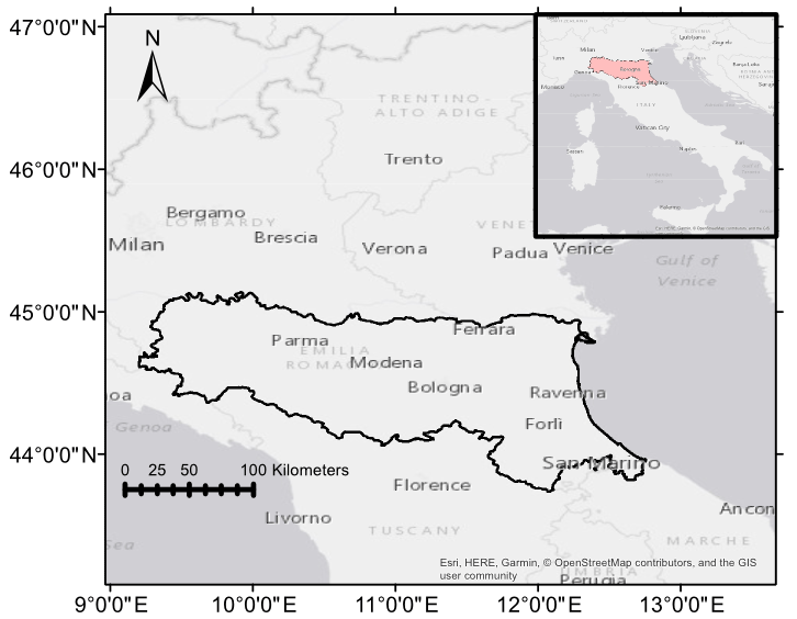
Figure 1 The geographical map of the Emilia-Romagna Region. The copyright of the background map belongs to © Esri (Light Gray Canvas Basemap).

For the soil moisture network in the region, currently, there is a total of 19 soil moisture sensors installed (all located in the plain area); however, only 1 of them can provide long-term continuous soil moisture monitoring datasets. The network is managed by the Regional Agency for Environmental Protection, Emilia Romagna Region. Through further investigations, it was found that a number of the sensors have actually never provided proper soil moisture measurements since the installation. Only one soil moisture sensor in the plain area is clearly not sufficient for any catchment-scale applications. Therefore, it is hoped that the proposed soil moisture network design scheme could provide some useful guidance to the local authority on an improved network in the future (i.e. a minimum number of sensors for reduced installation and maintenance cost, but at the right locations).

3 Methodologies

3.1 WRF model

The WRF model is a next-generation, non-hydrostatic mesoscale NWP system designed for both atmospheric research and operational forecasting applications (Skamarock et al., 2005). The model is capable of modelling a wide range of meteorological applications varying from tens of metres to thousands of kilometres (NCAR, 2020). Apart from the WRF's aforementioned advantage in including the catchment characteristics for the soil moisture estimations, it also has other merits that make it an ideal tool for providing the distributed soil moisture information for the network design. For instance, the WRF model's spatial and temporal resolutions can be changed depending on the input datasets to fit various application requirements, and a number of globally available data products can be selected to provide the necessary boundary and initial conditions for running the model. Therefore, WRF is able to provide valuable information for this study. Here WRF version 3.8 is used.

Table 1 WRF parameterizations used in this study.

3.1.1 Model parameterization

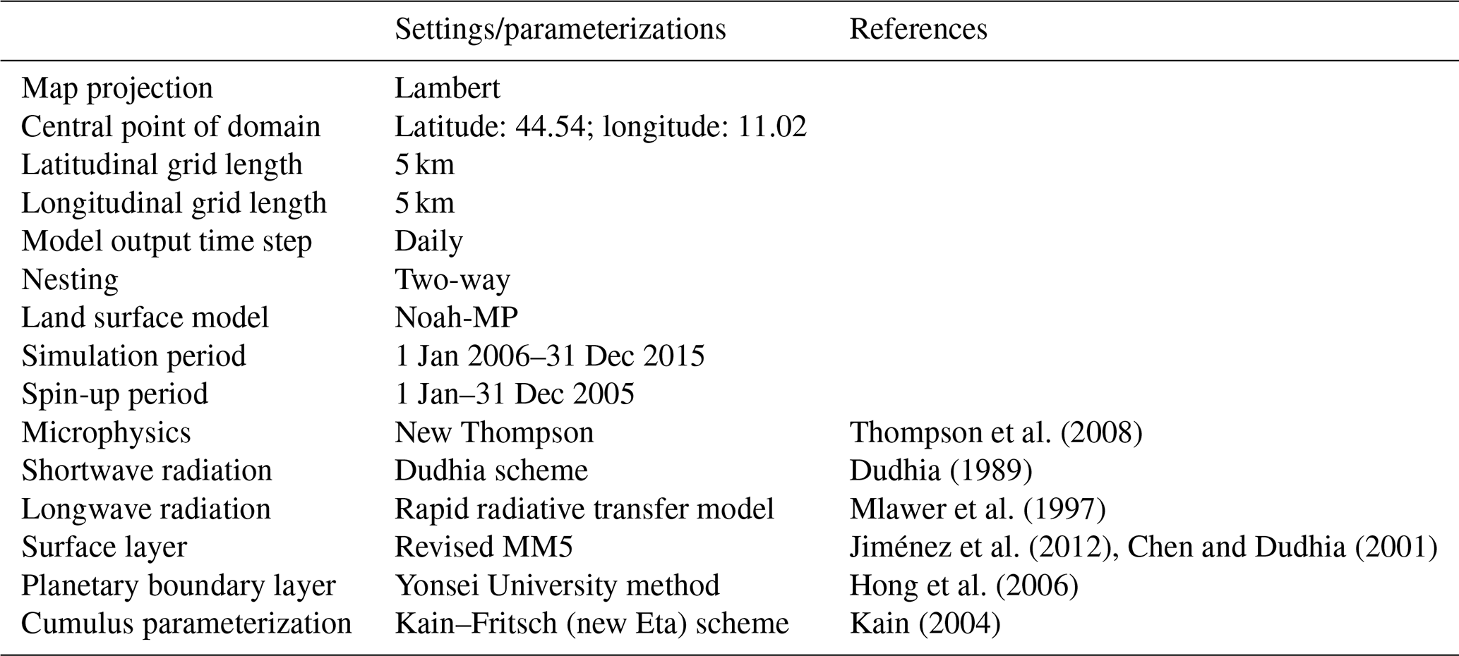
Apart from the atmospheric forcing, parameterization is also required to drive the WRF model. In particular, the microphysics scheme is important in simulating accurate rainfall information, which in turn is significant for estimating the accurate soil moisture fluctuations. WRF V3.8 supports 23 microphysics options, ranging from simple to more sophisticated mixed-phase physical options. In this study, the WRF Single-Moment 6-Class scheme is adopted which considers ice, snow, and graupel processes and is suitable for high-resolution applications (Zaidi and Gisen, 2018). The physical options used in the WRF setup are Dudhia shortwave radiation (Dudhia, 1989) and rapid radiative transfer model (RRTM) longwave radiation (Mlawer et al., 1997). Cumulus parameterization is based on the Kain–Fritsch scheme (Kain, 2004) which is capable of representing sub-grid-scale features of the updraft and rain processes, and such a feature is useful for real-time modelling (Gilliland and Rowe, 2007). The surface layer parameterization is based on the Revised fifth-generation Pennsylvania State University–National Center for Atmospheric Research Mesoscale Model (MM5) Monin–Obukhov scheme (Jiménez et al., 2012). The planetary boundary layer is calculated based on the Yonsei University scheme (Hong et al., 2006). In WRF, its land surface model plays a vital role in the integration of information generated through the surface layer scheme, the radiative forcing from the radiation scheme, the precipitation forcing from the microphysics and convective schemes, and the land surface conditions to simulate the water and energy fluxes (Ek et al., 2003). In this study, Noah Multiparameterization (Noah-MP) is chosen, because it has shown more accurate soil moisture estimation performance than the other two main schemes (Noah and CLM4) in other studies (Cai et al., 2014; Zhuo et al., 2019a). Table 1 shows the selected WRF parameterization schemes. The static inputs (i.e. land use and soil texture) are chosen in the WRF pre-processing package. Here, the land-use categorization is interpolated from the MODIS 21-category data classified by the International Geosphere Biosphere Programme (IGBP). The soil texture data are based on the Food and Agriculture Organization of the United Nations Global 5 min grid cell soil database.

3.1.2 Model setup

The WRF model is centred over the Emilia-Romagna Region and integrates three nested domains (D1–D3), with horizontal spacing of 45 km × 45 km (outer domain, D1), 15 km × 15 km (inner domain, D2), and 5 km × 5 km (innermost domain, D3). In this study, the innermost domain D3 is used (88×52 grids, west–east and south–north, respectively), with a two-way nesting scheme considered letting the information from the child domain be fed back to the parent domain. To drive the WRF model, the European Centre for Medium-Range Weather Forecasts (ECMWF) reanalysis (ERA-Interim) is adopted to provide the study region's boundary and initial conditions. ERA-Interim is a global atmospheric reanalysis that is available from 1979 to 2019 (ERA-5 as a recent update to ERA-Interim may also be used). The spatial resolution of the datasets is approximately 80 km on 60 levels in the vertical from the surface up to 0.1 hPa. It contains 6-hourly gridded estimates of three-dimensional meteorological variables and 3-hourly estimates of a large number of surface parameters and other two-dimensional fields. Please see Berrisford et al. (2011) for detailed documentation on ERA-Interim.

After the initialization, the model needs to be spun up to derive a physically valid state (e.g. equilibrium state) (Cai et al., 2014; Cai, 2015). In this study, WRF is spun up by running through the whole year of 2005. After the spin-up, the WRF model is run on a daily time step from 1 January 2006 to 31 December 2015, using the ERA-Interim datasets. The modelled WRF grids within the Emilia-Romagna catchment (total of 828 grids) are shown in Fig. 2 as black dots, with the elevation map also illustrated in the background. For exploration purposes, this study uses the WRF surface soil moisture at 0–10 cm for the network design. This is because the surface soil moisture changes more frequently in comparison with the root-zone soil moisture. And in theory, the root-zone soil moisture should follow the general trend of the surface soil moisture (in a delayed mode). In our future study, the WRF root zone soil moisture will also be explored.

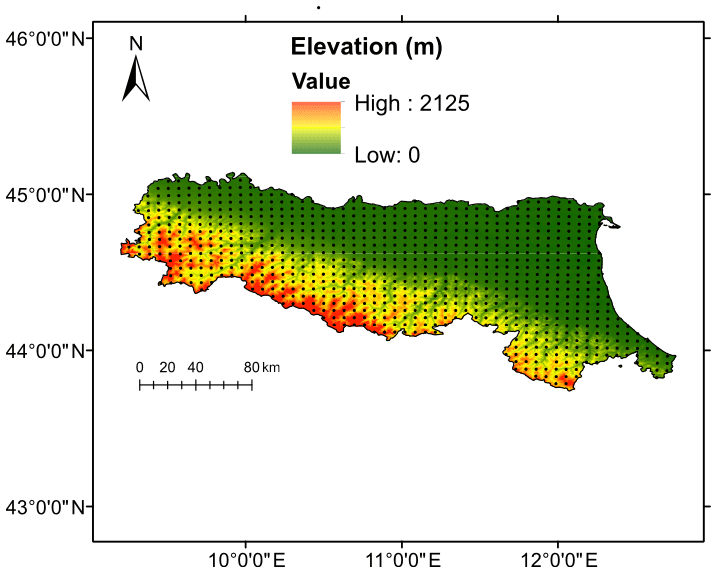
Figure 2 WRF grids used in the analysis, with the DEM map in the background.

3.2 Soil moisture network design

For the soil moisture network design, three main problems need to be tackled. The first is how redundant the network is, the second is how many soil moisture sensors are needed within a catchment, and finally where the best locations are to place them. To solve the first problem, PCA is used to investigate the redundancy degree of the network. To solve the latter two problems, the K-means CA is adopted. It should be noted that the information used for the PCA/CA is based on the soil moisture temporal variations (e.g. the 10-year time series data), so that areas following similar soil moisture variations can be grouped together, and location information is not used here. However, due to the influence of local characteristics, the resultant clusters should more or less reflect the geographical feature.

3.2.1 PCA for network redundancy analysis

When soil moisture data are collected from p soil moisture sensors, these data are often correlated. This correlation reflects the complexity of the catchment and indicates that some of the information collected from one sensor is also contained in the remaining p−1 sensors (Gangopadhyay et al., 2001). The role of the PCA is to examine the redundancy of the WRF 5 km gridded soil moisture outputs (Dai et al., 2017). PCA is a statistical procedure for multivariance feature extraction. It adopts an orthogonal transformation to convert a set of possibly correlated observations into a set of linearly uncorrelated variables called principal components. This transformation is defined in such a way that the first principal component has the largest possible variance, and each succeeding component in order has the highest variance possible under the constraint that it is orthogonal to the preceding components (Wold et al., 1987).

In this study, we have p WRF soil moisture grids with N observations (the time series of the data, i.e. 10-year daily datasets). The covariance matrix p×p can be calculated which is denoted as X, and the eigenvectors and the eigenvalues of the matrix can also be determined, correspondingly. Since eigenvectors of X are orthogonal, the p eigenvectors are used to construct the principal components, which can be represented as

$$\begin{array}{}\text{(1)}& \mathrm{eigenvector}=\left({\mathrm{eig}}_{\mathrm{1}}{\mathrm{eig}}_{\mathrm{2}}{\mathrm{eig}}_{\mathrm{3}}\mathrm{\dots }{\mathrm{eig}}_p\right).\end{array}$$

With such a relationship, the original datasets can be transformed in terms of eigenvectors into a new dataset Z. Z is shown as the following:

$$\begin{array}{}\text{(2)}& Z_i=X_{\mathrm{1}}{\mathrm{eig}}_{i,\mathrm{1}}+X_{\mathrm{2}}{\mathrm{eig}}_{i,\mathrm{2}}+\mathrm{\dots }+X_p{\mathrm{eig}}_{i,p},i=\mathrm{1},\mathrm{\dots },p,\end{array}$$

where Z_i is the new dataset and X_i is the original dataset. The variance of each of the components is the eigenvalue. The eigenvector with the highest eigenvalue is the principal component of the dataset. Since the optimal number of principal components is dependent on the amount of original variance the network should retain, the examination of the network redundancy is implemented based on the desired rate of variance contribution, and the number of principal components can thus be calculated correspondingly.

3.2.2 K-means cluster analysis (CA) for sensor number and placement determination

After exploring the redundancy level of the network, it is necessary to determine how many WRF grids to select so that the maximum level of information can be retained. Similarly to the relationship between the number of principal components and the variance contribution rates, the appropriate number of grids is also dependent on the amount of original variance the network would like to retain. Since the number of components from the PCA does not directly represent the physical number of grids, we propose to use the elbow method to find the corresponding number of grids. The elbow method is based on K-means clustering and looks at the variance contribution rate as a function of the number of grids. Generally, the required number of grids increases when the variance contribution rate increases. However, the growth rate is not constant and changes significantly at a critical point (threshold), which is used in this study as the desired rate for the soil moisture network design. If for a specific desired variance the determined number of grids is significantly less than the total number of WRF soil moisture grids, then it can be concluded that the network is heavily redundant, and even by removing a large number of grids, the rest can still provide sufficient soil moisture information for the entire catchment and vice versa. In this paper, the variance contribution rate of 70 %–99 % is tested.

The K-means approach is a typical distance-based clustering method which uses the distance as the indicator of similarity among objects (i.e. the smaller the distance, the higher the similarity of two objects) (Kodinariya and Makwana, 2013). In this study, the Euclidean distance is adopted as the distance measurement. It is a simple and widely used way of calculating the distances between objects in a multidimensional space (Danielsson, 1980). The centroid of each cluster is the point at which the sum of Euclidean distances from all objects in that cluster is minimized. It is an iterative approach repeated for all of the clusters.

After deciding on the number of soil moisture grids from the elbow method and setting up the optimal clusters, we propose two ways to find the most suitable grid for the sensor placements. One way is by finding the grid which gives the median averaged soil moisture (i.e. averaged over the whole study period) in each of the clusters (denoted as CA-Med), and another is by identifying the maximum averaged soil moisture in each of the clusters (denoted as CA-Max) (Dai et al., 2017). CA-Max is focused on extreme soil moisture conditions, whilst CA-Med is focused on the median condition. Since they provide results in two aspects, it is useful to explore both in this study. As a result, for each cluster, there is one optimal grid and, grouped with the other optimal grids found in other clusters, the ideal placements for the soil moisture sensors are identified. The group of the selected grids is considered to be the optimal combination of locations that can provide the desired variance of the original WRF soil moisture measurements over the whole catchment.

3.3 Network evaluation

Since there is no existing optimal in situ soil moisture network that can be used as a reference for the evaluation, it is challenging to assess the designed network performance based on a comparison study. However, the designed network should be efficient enough to represent the maximum amount of information with the minimum number of sensors within a catchment. In other words, the designed network should retain the main catchment-scale soil moisture information of the original WRF's full outputs, which is particularly important for the hydrological modelling. To assess the network in such an aspect, the soil moisture information contained by the designed and original networks is compared. Two statistical indicators are used for this purpose, namely the Pearson correlation coefficient and the Nash–Sutcliffe coefficient.

The Pearson correlation coefficient (r) is a statistical measure of the linear correlation between two datasets, which in this study can estimate the systematic deviation between the designed (S_d) and original (S_o) catchment-scale soil moisture variations, and it is calculated by the following equation:

$$\begin{array}{}\text{(3)}& r_{S_{\mathrm{o}},S_{\mathrm{d}}}={\displaystyle \frac{E\left[S_{\mathrm{d}}{S}_{\mathrm{o}}\right]-E\left[S_{\mathrm{d}}\right]E\left[S_{\mathrm{o}}\right]}{\sqrt{\left(E\left[S_{\mathrm{d}}^{\mathrm{2}}\right]-E{\left[S_{\mathrm{d}}\right]}^{\mathrm{2}}\right)\times \left(E\left[S_{\mathrm{o}}^{\mathrm{2}}\right]-E{\left[S_{\mathrm{o}}\right]}^{\mathrm{2}}\right)}}},\end{array}$$

where E is the mean value of the corresponding vector. In this study, the optimal performance is achieved when $r_{S_{\mathrm{o}},S_{\mathrm{d}}}$ equals 1.

Nash–Sutcliffe efficiency (NSE) (Nash and Sutcliffe, 1970) is used widely in hydrology to evaluate the prediction accuracy in hydrological modelling, which can be obtained by

$$\begin{array}{}\text{(4)}& \mathrm{NSE}=\mathrm{1}-{\displaystyle \frac{\sum {\left(S_{\mathrm{o}}^t-S_{\mathrm{d}}^t\right)}^{\mathrm{2}}}{\sum {\left(S_{\mathrm{o}}^t-E\left[S_{\mathrm{o}}\right]\right)}^{\mathrm{2}}}},\end{array}$$

where t is the time step of the dataset. The NSE range is [1, −∞). The closer NSE is to 1, the more accurate the designed network is.

Figure 3 Cross-correlation matrix for the whole catchment.

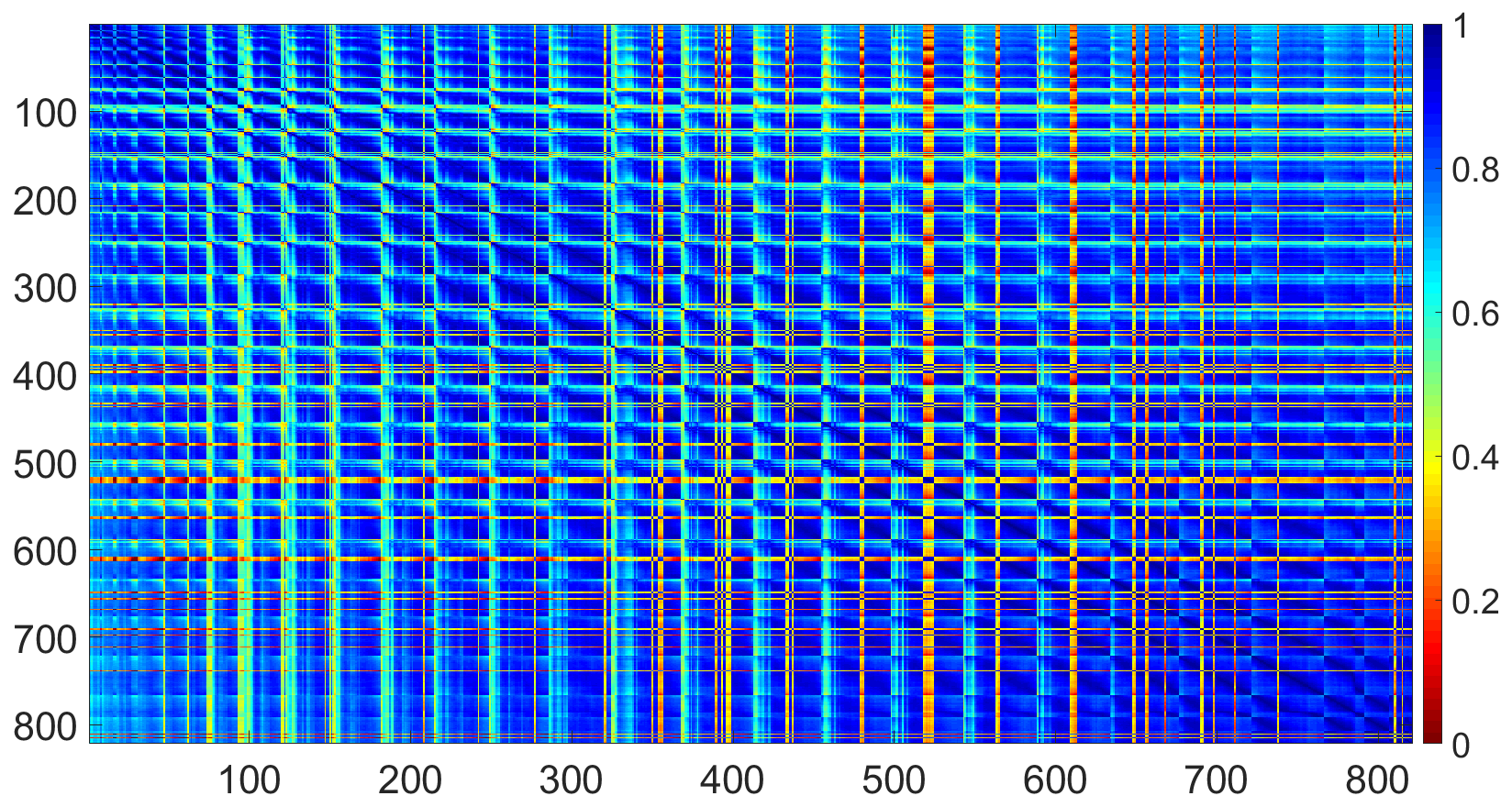
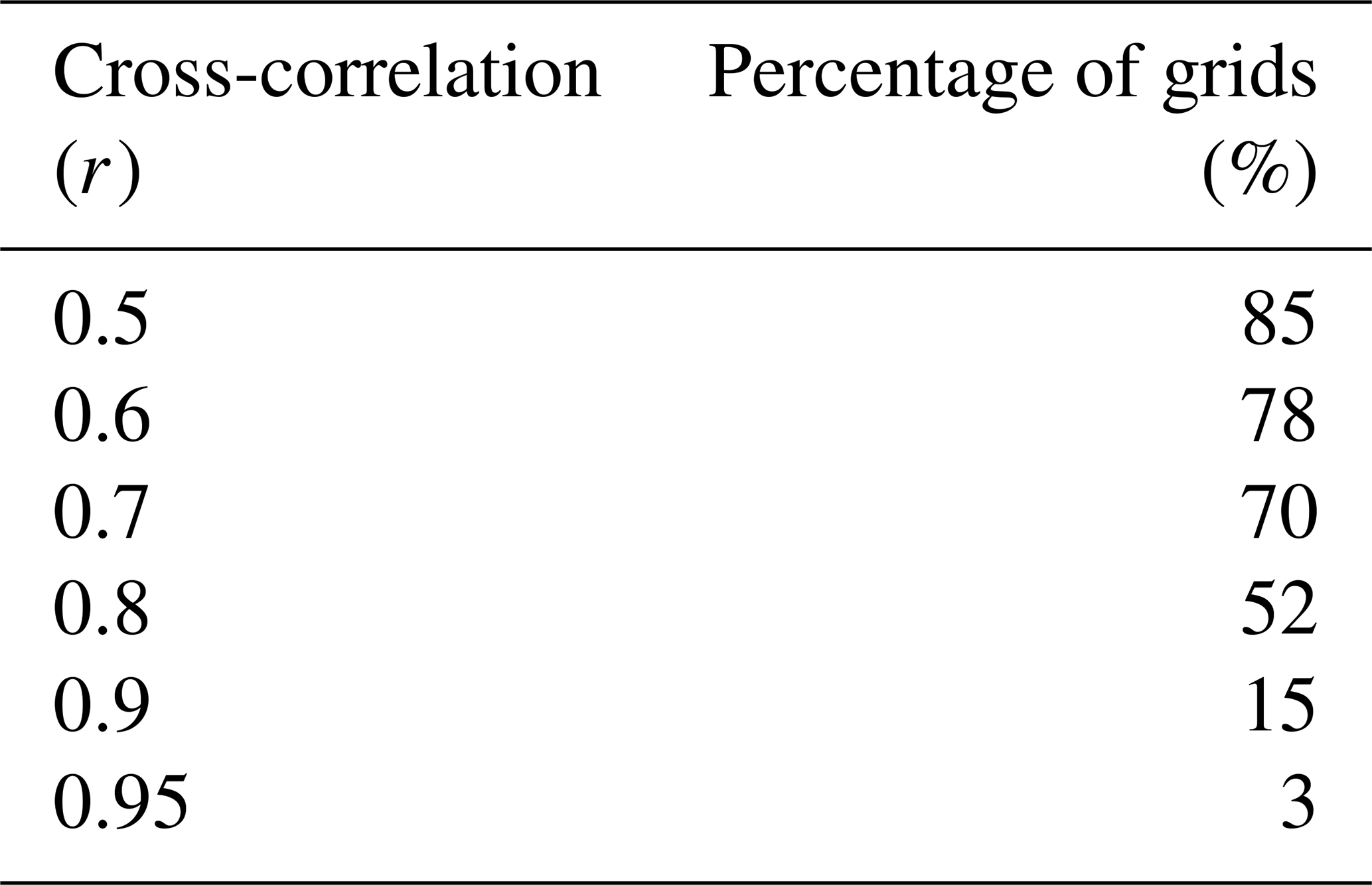
Table 2 The relationship between the percentage of grids and the cross-correlation.

4 Results

4.1 Soil moisture network redundancy analysis

Within the study area of 22 124 km², there is a total number of 828 WRF soil moisture grids. With such a dense dataset, there should exist information redundancy. To explore this, a cross-correlation (r) matrix for all of the grids over the whole study period is plotted in Fig. 3. It can be seen that the majority of the matrix is in blue tone, which means most of the grids (85 %) are correlated (r>0.5) with most of the others (as shown in Table 2). In addition, over half of the grids (52 %) have high correlation (r>0.8) with the rest of the grids, and even 15 % of the grids can achieve very high correlation (r>0.9). However, it is clear from the map that some grids (e.g. grid numbers 396–398 and 523–529) are less strongly correlated with the others (red tone, with low correlation < 0.3 observed), which means more soil moisture sensors might need to be installed at those locations. A further exploration of cross-correlation performance using boxplots is shown in Fig. 4b. The locations of the selected grids (as in Fig. 4b) are marked in Fig. 4a with red circles. It can be seen that the nine grids are distributed evenly within the catchment in order to represent a spectrum of catchment features (different land covers, elevations, soil types, etc.). From the boxplot, it can be seen for a specific grid that the cross-correlation can range from as low as below 0.1 to as high as almost 1. The large range is particularly obvious for Grid 500, which is located in the plain zone near the eastern boundary of the catchment and is close to the Valli di Comacchio lagoon. The closeness to the waterbody could mean its soil moisture is dominated more by the shallow water table at that location, which makes the soil moisture relatively insensitive to the weather in comparison with grids located further away. For Grid 100, its correlation with the rest of the grids in the catchment is relatively low, with 75 % of the cross-correlations less than 0.6. The potential reason could be that because it is located in the southern mountainous zone, with a high density of tree coverage and complex topographic conditions, its soil moisture changes more differently than the other grids. A similar condition is observed for Grid 1, which is also located in a hilly zone on the southern boundary of the catchment (i.e. lower correlation as shown in the boxplots). Such a phenomenon is not unexpected and could mean more sensors are needed in those complex zones for better soil moisture monitoring purposes. However, for grids like 300 and 600 (and the surrounding areas), since the majority of their correlations are high and they are located in plain areas with no water boundary nearby, they could be arranged with a smaller number of soil moisture sensors.

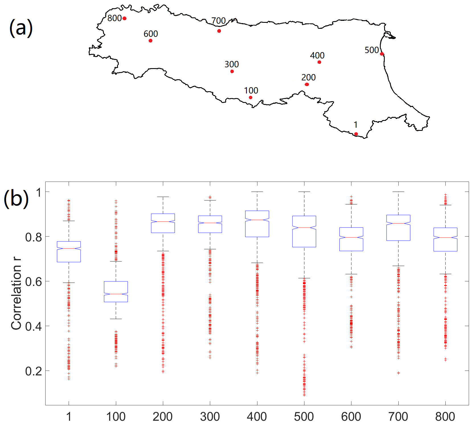
Figure 4 (a) WRF selected grid number; (b) correlation boxplot for the selected grids as highlighted in red in (a). For the boxplot, it shows the minimum, maximum, 0.25th, 0.50th, and 0.75th percentiles, and outliers (red cross).

4.2 PCA and sensor number

In summary, through the cross-correlation exploration, many parts of the WRF soil moisture dataset are significantly redundant. To systematically investigate the redundancy degree of the network, the PCA approach is applied. Figure 5a shows the PCA results to provide useful guidance on the acceptable loss of information. It is clear to see that the first principal component carries close to 80 % of the total variance, with the second component bringing this to nearly 90 %. This result again indicates that high redundancy exists in the dataset, and just one component can contain almost 80 % of the total soil moisture information. To better understand the relationship between the principal component numbers, the variance contribution rate, as well as the corresponding required number of grids (through the elbow method), a set of variance contribution rates from 70 % to 97.5 % is used as the representatives. The required number of components and the grids are listed accordingly in Table 3. It can be seen that only one component with six grids is sufficient to retain 70 % of the soil moisture information. Even when the variance is set at 80 %, only two components are needed to meet the requirement, and the corresponding number of soil moisture girds is 11 (1.3 % of the total grids). To satisfy 90 % variance, three components are needed, and although the total number of grids is increased to 50, it is still significantly less than the WRF's full inputs. The detailed numbers further indicate the relatively high level of redundancy in the WRF's original dataset.

Figure 5 (a) PCA and (b) elbow curve.

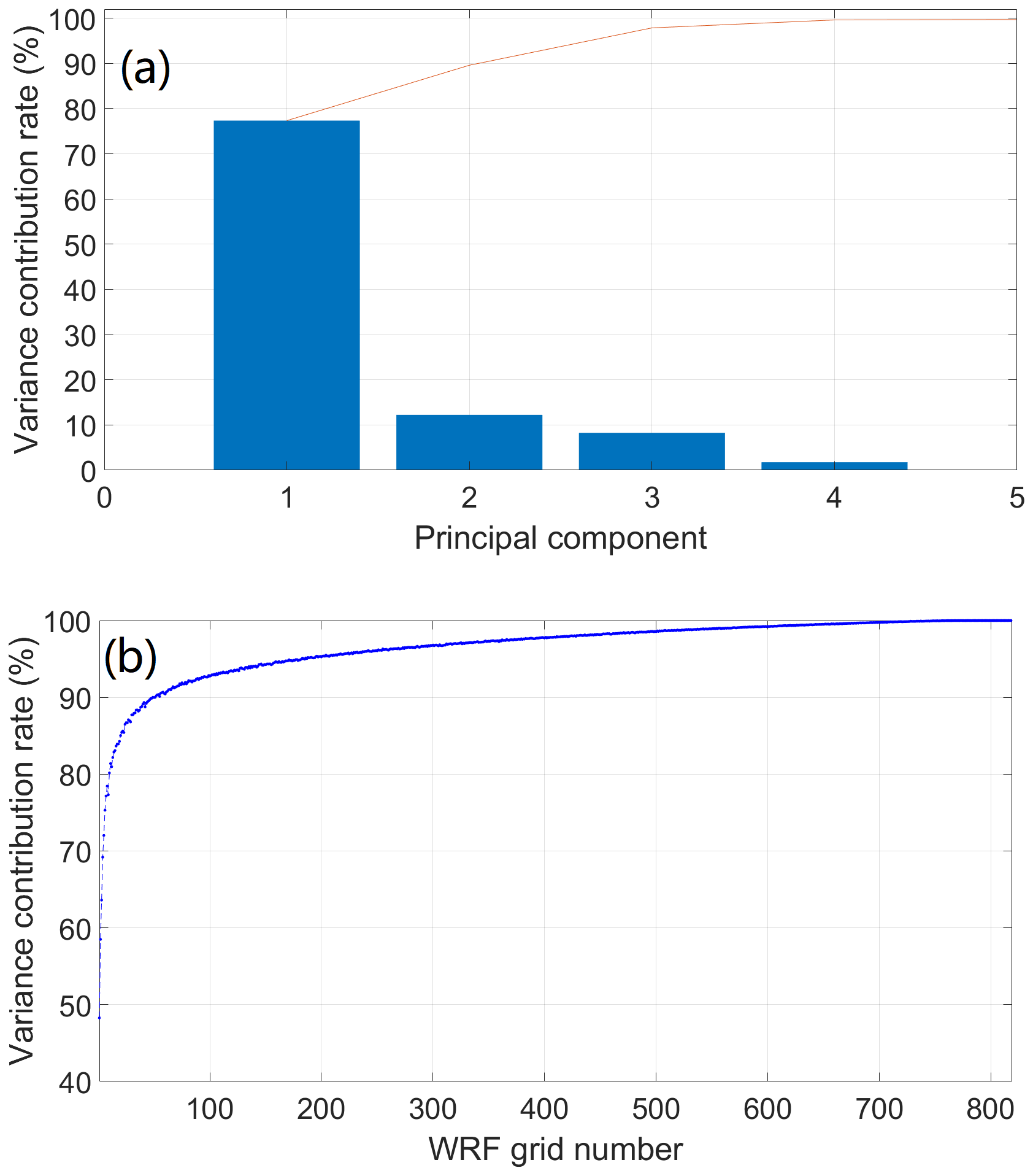
Table 3 The number of components and grids to reach the % variance threshold (based on the PCA method and the elbow curve method).

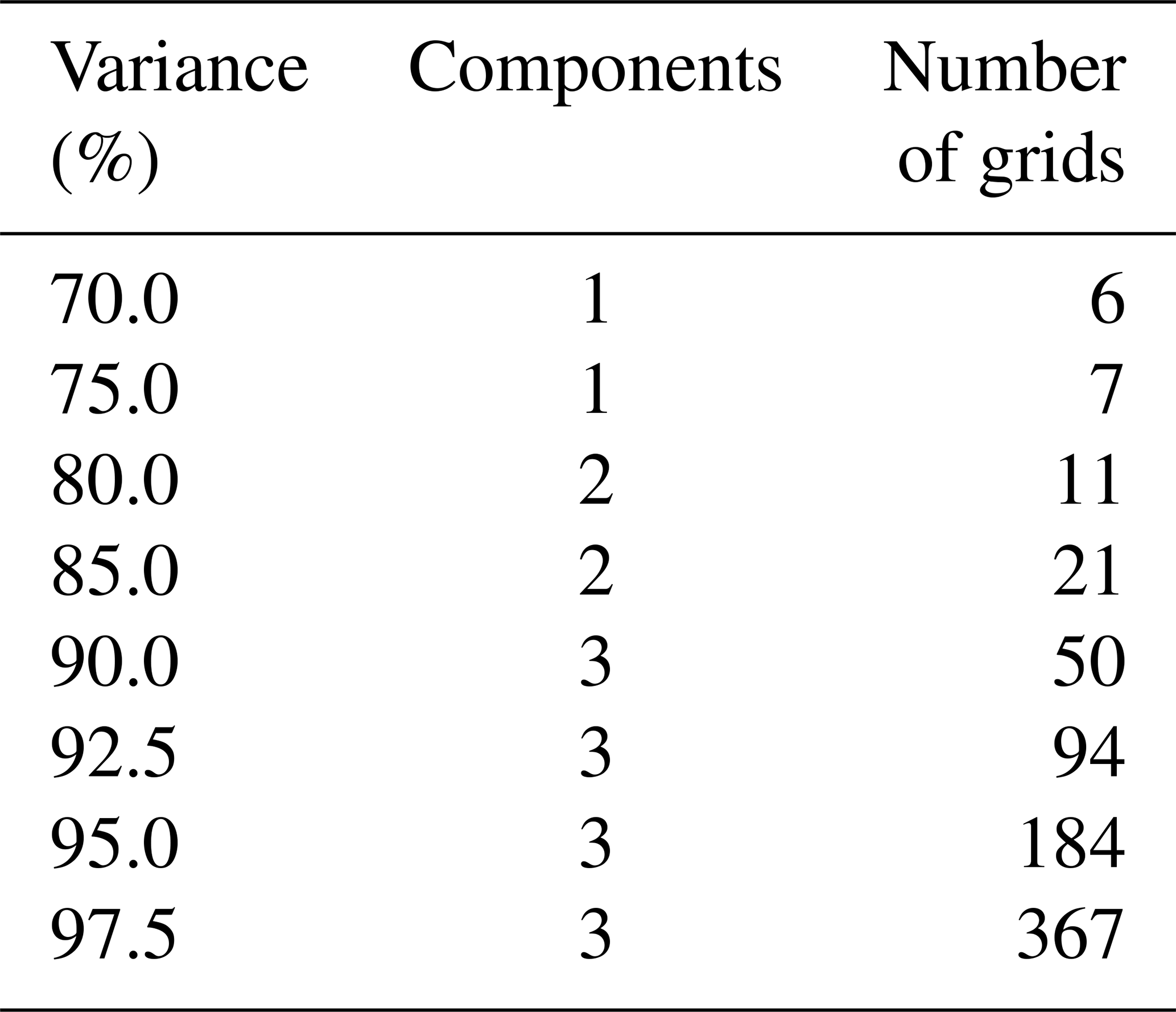
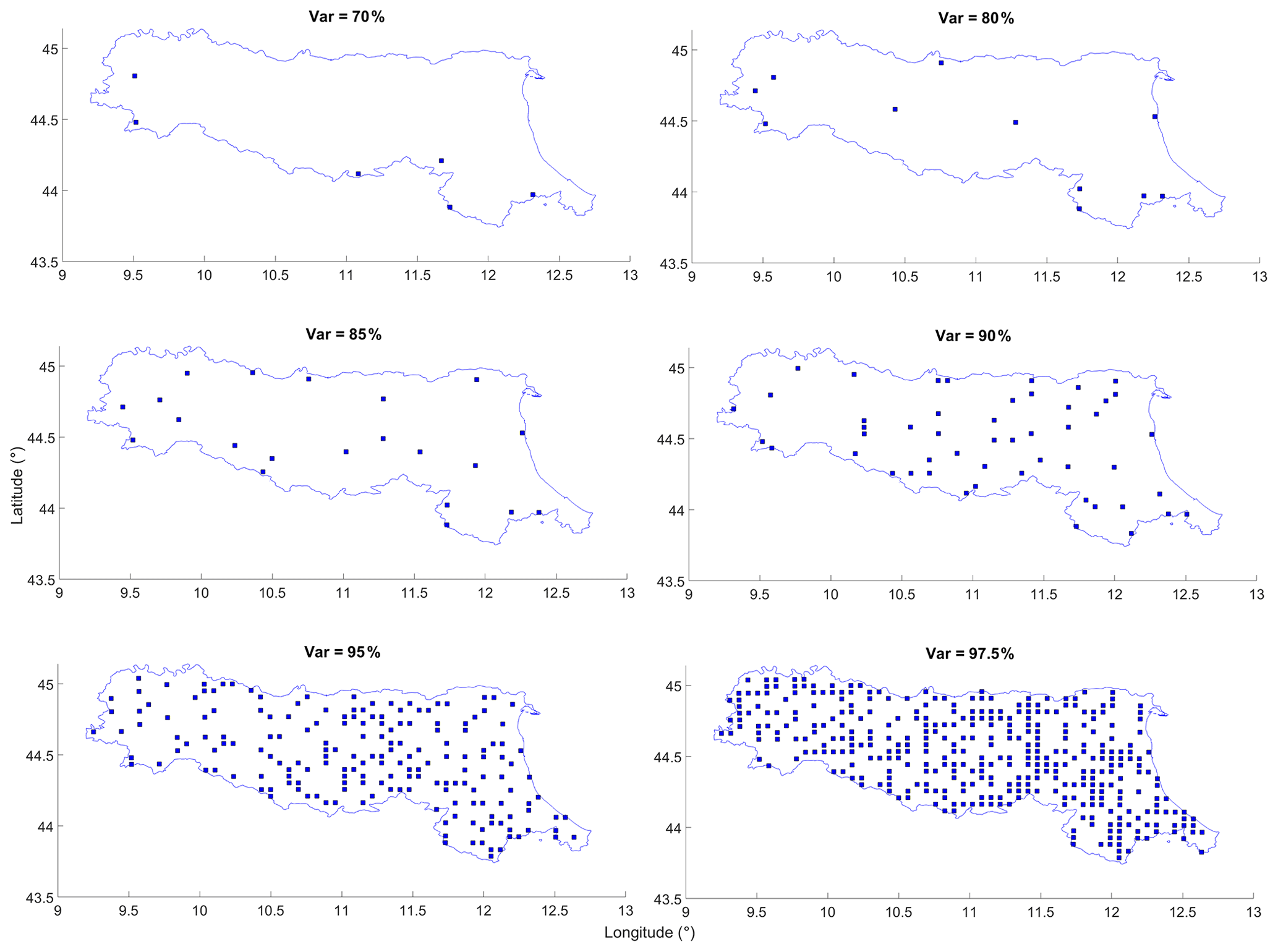
Figure 6 Designed soil moisture sensor locations, based on CA-Max. The total numbers of grids used for the design are 6, 11, 21, 50, 184, and 367 for 70 %, 80 %, 85 %, 90 %, 95 %, and 97.5 % variance, respectively.

The trend can also be observed through the elbow curve which is illustrated in Fig. 5b. It presents the relationship between the variance and the number of grids. It can be seen to meet the increment of variance; the required number of grids also increases. But the growth rate is the most significant when the variance is smaller than 70 %, and it then slows down gradually after that. When the variance is 95 %, the rate is further weakened. Based on the curve, it is suggested that the desired variance (i.e. trade-off point) is between 80 % and 95 %. The required number of soil moisture grids for 80 %, 85 %, 90 %, and 95 % is 11, 21, 50, and 184, respectively. It is clear that, in order to achieve the 95 % variance, a significantly greater number of additional grids are required, that is, 268 % more than for the 90 % variance case. Therefore, for further improvement of variance from 90 % to 95 %, the economic cost for the additional number of sensors might not be as valuable as for the 85 % to 90 % case (138 % additional sensors are required for the enhancement).

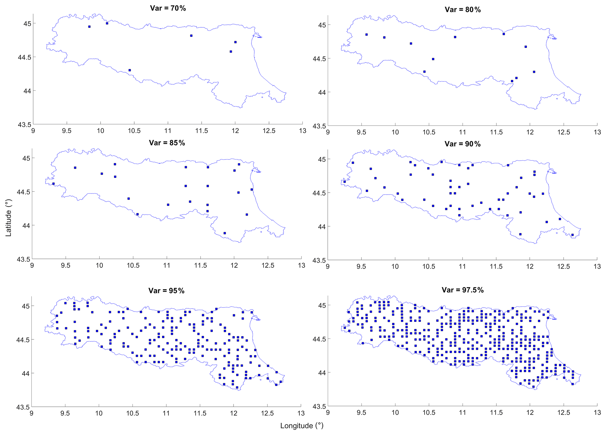
Figure 7 Designed soil moisture sensor locations, based on CA-Med. The numbers of grids used for the design are 6, 11, 21, 50, 184, and 367 for 70 %, 80 %, 85 %, 90 %, 95 %, and 97.5 % variance, respectively.

4.3 Soil moisture sensor location design

Once the degree of redundancy for the full WRF soil moisture network is established, the next step is to determine the optimal locations for sensor placements. Here, CA-Max and CA-Med are used. The designed networks for CA-Max and CA-Med are illustrated in Figs. 6 and 7, respectively. The indicated locations in the figures provide guidance on the preferential areas for the soil moisture sensor placements. Each of the methods gives a different set of sensor locations; for instance, the selected optimal soil moisture grids from the CA-Max method tend to be located at the catchment boundary, and the situation is particularly obvious for the low-variance cases (i.e. 70 %–80 %). For example, when the variance is set at 70 %, the selected optimal locations from CA-Max are mostly distributed near the catchment's southern boundary, while from CA-Med, it is more homogeneously distributed (i.e. one at the southern boundary, one in the north, two in the north-western part, and two in the north-eastern part). This is because CA-Max selects the maximum averaged soil moisture of a cluster. In the case study area, since the southern boundary of the catchment is mainly covered by dense trees which generally have higher soil moisture contents than the rest of the catchment, the selected locations tend to distribute near the southern boundary. For CA-Med, as it selects the median averaged soil moisture of a cluster, the resultant locations are more evenly distributed.

When the variance is increased, for instance at 90 %, the difference between the two CA methods becomes less distinctive. Despite this, it can still be seen for CA-Max that there is less coverage of sensors in the western and eastern parts of the catchment, with most of the sensors located in the mid-region. However, for the same variance, the sensor distribution from CA-Med looks more evenly distributed visually. Nevertheless, when the variance reaches as high as 97.5 %, the difference from the two methods becomes rather small, as 367 sensors are located covering most parts of the catchment in both cases.

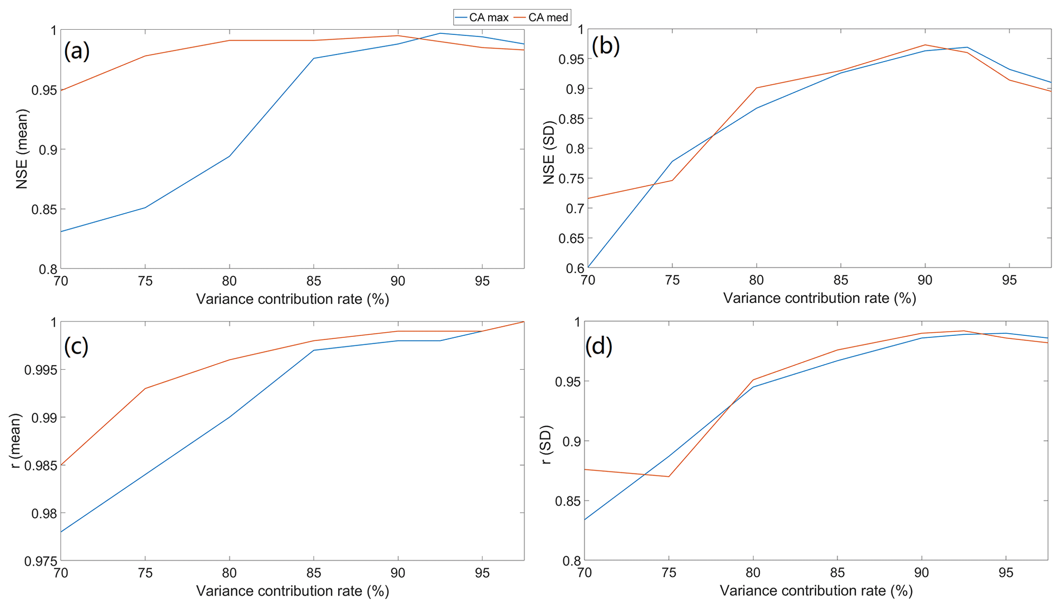
Figure 8 NSE and r plots: (a) NSE performance based on the areal mean soil moisture, (b) NSE performance based on the areal standard deviation soil moisture (STD), (c) r performance based on the areal mean soil moisture, and (d) r performance based on the areal standard deviation soil moisture.

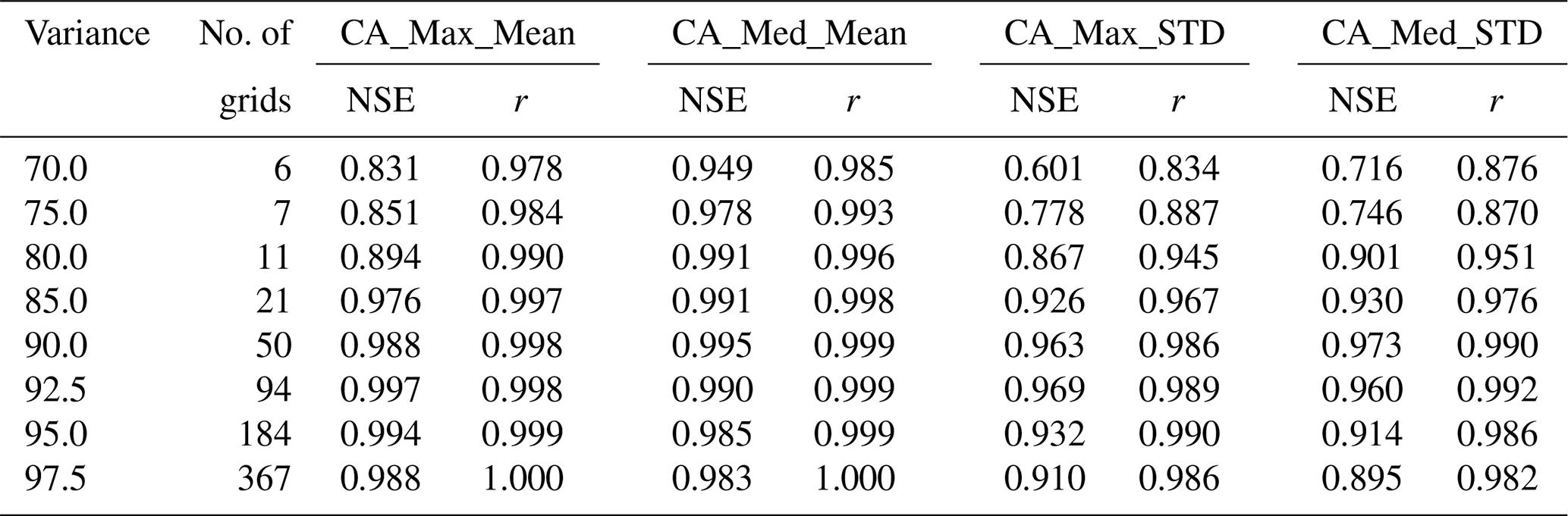
Table 4 NSE and correlation r performance of CA_Med and CA_Max.

4.4 Soil moisture network evaluation

The evaluation of the designed network is challenging, as there are no standard assessment criteria available to guide on what kind of network is the most appropriate for a given study area. In essence, the designed network should be efficient, which means the network should contain the maximum amount of information with a minimal number of sensors. In this study since we focus on the soil moisture's hydrological applications (catchment scale), to evaluate the efficiency of the proposed schemes, the catchment-scale soil moisture data derived by the designed networks are compared with the WRF's full inputs (828 grids). Both the areal spatial mean and standard deviation are calculated. The Pearson correlation coefficient and the Nash–Sutcliffe coefficient are used to quantify the relationships between the two soil moisture datasets. The results for both CA-Med and CA-Max are compared in Fig. 8. Based on the areal mean soil moisture (Fig. 8a and c), it is clear to see that CA-Med outperforms CA-Max for the majority of the variance cases (both NSE and r), except for the NSE results when the variance is over 90 %. Moreover, for the NSE results, a decline in the performance can be observed clearly after it passes the 90 % variance point, which illustrates that an increment of the sensor number does not necessarily mean an improvement of the performance. For the standard deviation, the disparity between the two methods is smaller. When the variance is below 80 %, the growth trend for the CA-Med case is not clear, as it firstly drops at the 75 % point and then climbs up again when the variance increases, whereas for the CA-Max case, there is a clear upward trend. Similarly to Fig. 8a, it is interesting to see that for the areal standard deviation in Fig. 8b and d, the NSE and r also start to drop after reaching around 90 %. The evaluation results are summarized in Table 4 for numerical comparison. Since CA-Med surpasses CA-Max for most of the cases, it is chosen for the network design. In the aspect of the desired variance, because as discussed earlier, when the variance climbs over 90 %, the performance instead drops. Therefore 90 % variance is suitable for use in the network design in this case.

The time series plots of the areal soil moisture mean and standard deviation are shown in Fig. 9. Generally, the designed network can estimate the catchment's mean soil moisture very well, as it follows the variation of the WRF's full input dataset closely (NSE = 0.995 and r=0.999). For the standard deviation, the general trend from both datasets shows a higher spatial variation of soil moisture over the dry season and lower variation during the wet season. The spatial variation is averaged around 0.04 m³ m⁻³ throughout the whole study period. However, there are some disparities between the two datasets; in particular, during the wet season (bottom peaks in the STD plot), the designed network on several occasions overestimates the spatial soil moisture variation, and during the dry season (top peaks in the STD plot), it underestimates it instead. Nevertheless, the differences are small and the correlation between the two datasets is high, with NSE = 0.973 and r=0.990 obtained. In conclusion, the designed network can maintain the dominant information of the WRF's full-grid input well.

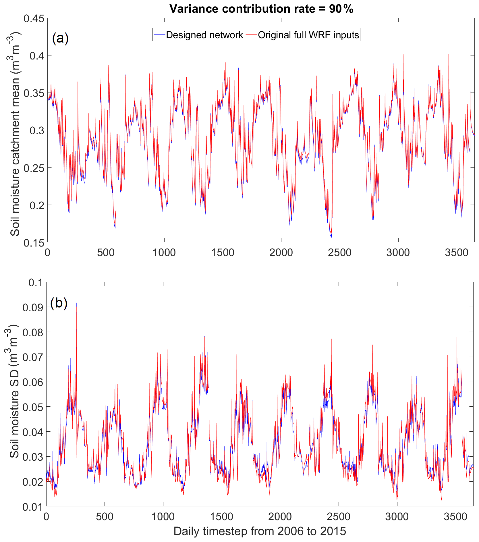
Figure 9 (a) The areal mean soil moisture of the designed and WRF full-input networks and (b) the areal soil moisture standard deviation of the designed and WRF full-input networks. The designed network is based on CA-Med, 90 % variance contribution rate, and 50 sensors.

Figure 10 Comparison between the existing and designed soil moisture networks.

The sensor displacements for the designed and existing (in situ) networks are illustrated in Fig. 10. In comparison with the distribution of the proposed network, the existing network is clearly biased, with all of the sensors located in the mid-plain zone only. Such a distribution (i.e. no sensors located in the southern mountainous (highly vegetated) region) can have adverse impacts on the accuracy of the areal mean soil moisture estimation. However, we can see that some of the existing sensors are located near some of the designed sensors, which could be kept if located within the same cluster. But a lot more sensors are indeed required in the hilly zone, where currently no sensors are installed. The existing stations could be initially installed for irrigation purposes, which are hence mainly located in the plain area. Scatterplots of the areal mean soil moisture calculated from the designed and existing networks are also presented in Fig. 11. The performance difference between the two networks is clear to observe. For the proposed network, the points are located close to the identical line, whereas for the existing network, due to the inappropriate sensor distributions over the catchment, the points are more dispersive (NSE = 0.889). The performance of the existing network (i.e. using WRF grid data from the existing locations) in comparison with the proposed networks is worse; in particular, its NSE is lower than the 70 % CA-Med case in the designed network (i.e. 0.949). For the existing network, without putting sensors in the highly vegetated region, the network clearly underestimates soil moisture variations during the dry season (i.e. for the cases when the soil moisture is less than 0.25 m³ m⁻³).

Figure 11 Scatterplots for areal mean soil moisture: (a) WRF full grid inputs against the proposed network (NSE = 0.995, r=0.998); (b) WRF full grid inputs against the existing in situ network (NSE = 0.889, r=0.987).

5 Discussions and conclusions

With the low-cost soil moisture sensors becoming more and more available and modern communication technology (i.e. Internet of Things), it is expected that more in situ soil moisture sensors will be installed in the future. Although there is a wide range of soil moisture networks around the world (e.g. USA NSMN, ISMN, USA state Mesonets), the majority of them are not purposely designed for catchment-scale hydrological studies. Moreover, to our knowledge most existing soil moisture network studies are based on using in situ/aircraft datasets in small experimental areas, which can hamper their applications in data-sparse regions. In this paper, a low-data requirement scheme (only WRF-simulated soil moisture information is required, which can be generated globally) together with simple statistical analysis (PCA/CA) is proposed to overcome the aforementioned shortcomings. Through a series of evaluations of the developed network, it can be concluded that the method can provide efficient catchment-scale soil moisture estimations (i.e. high accuracy of the areal mean and standard deviation soil moisture estimations). To retain 90 % variance, a total of 50 sensors in a 22 124 km² catchment is needed. In comparison with the original number of WRF grids (828 grids), the proposed network requires a significantly smaller number of sensors. Furthermore, in comparison with the existing soil moisture network in the Emilia-Romagna Region, the proposed network has sensors more evenly distributed, covering most representative parts of the catchment (e.g. both plain and mountainous regions), and can obtain more accurate catchment-scale soil moisture estimation. However, several points need to be discussed as follows.

The first point is about the uncertainty of the WRF's soil moisture estimations, which could influence the accuracy of the network design. It is acknowledged that the reliability of the designed network is influenced by the performance of the WRF model. To evaluate the WRF results and test whether the proposed network can reproduce the catchment-scale soil moisture well, a long-term densely covered soil moisture network will be required. Setting up such a network is challenging and difficult to realize due to the high installation and maintenance cost. In this study, a long-term WRF soil moisture estimation with 1-year spin-up time is used which could to some extent produce a more stable result. But since “All models are wrong” (by George E. P. Box, https://en.wikipedia.org/wiki/All_models_are_wrong, last access: 14 May 2020), an uncertainty model (Zhuo et al., 2016) could be proposed to be integrated with the network design scheme. For example, we can generate a large number of probable “true soil moisture” datasets based on the proposed uncertainty model so that a set of possible soil moisture networks can be produced. As a result, the designed network will be expressed in a probabilistic form instead of a determinate form. In addition, a decision-making scheme considering different conditions (e.g. accessibility, installation, and maintenance cost) under the uncertainty can be developed to select the most suitable soil moisture network. The uncertainty influence of the WRF soil moisture on the network design will be investigated in future studies.

Second, the case study is based on the daily soil moisture inputs for the hydrological applications. With different research needs (meteorology, climatology, hydrology, water resources, geology, etc.), various temporal scales of soil moisture data might be required; for example, climate change study requires soil moisture data in decades or hundreds of years, which often needs annual-scale measurements; drought assessment requires monthly to seasonal datasets; while for hydrometeorological prediction applications, hourly datasets might be needed. For the network design, the input data's temporal scale (daily, weekly, monthly, yearly) can influence the final network design; therefore, it is worth investigating in future studies about the temporal-scale effect on the network design.

Third, for a complex catchment like Emilia-Romagna, other uncertainty sources apart from the WRF model can also affect the performance of the designed network; for instance, the study area has varied climate conditions (a mixture of subcontinental and cool temperate) and distinct seasonal changes (wet/dry seasons). Therefore, separating/combining networks under different catchment conditions could result in an improved soil moisture network design. Furthermore, the poor accessibility to sensors is another challenging point that can hamper the performance of the designed network in real life. To overcome the accessibility issue, advanced soil moisture sensors (e.g. Cosmic-ray soil moisture sensor; Zreda et al., 2012) with low maintenance requirements could provide a good alternative for long-term deployment in complex terrain. Moreover, the accessibility factor could also be considered for the network design (e.g. can be considered during the CA for the sensor placements).

Fourth, the proposed method assumes that a soil moisture station placed inside a 5 km grid cell can perfectly represent the mean soil moisture condition for that grid cell. However, in reality it is not the case. As a result, the scale mismatch between the footprint of an in situ point-based soil moisture station and the 5 km dataset used here would be expected to degrade the performance of the resulting network (Crow et al., 2012). Advanced soil moisture sensing technology as aforementioned, such as the Global Navigation Satellite Systems (GNSS) and the Cosmic-ray, could provide alternative solutions over point-based sensors to reduce such impacts. In particular, the COSMOSUK (Evans et al., 2016) network is moving towards integration with operational weather forecasts, and Cosmic-ray is suitable to be used in complex terrain and might be a good option to be used for a national network as compared with point-based in situ sensors.

Fifth, regarding the temporal variation factor, as has been mentioned earlier, the information we used for the PCA/CA is based on the soil moisture temporal variations, so that areas following similar soil moisture temporal variations can be identified. Although location information is not used for the PCA/CA analysis, due to the influence of local characteristics, the resultant clusters should more or less reflect the geographical feature. The resultant clusters are shown in Fig. 12. It can be seen that most of the clusters are geographically connected. Although k-means has issues in dealing with nonconvex clusters and geographically there might exist nonconvex-shaped clusters, as demonstrated in this paper k-means indeed is very useful for the soil moisture network design (the time series datasets are used instead of the location information).

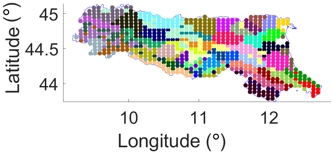
Figure 12 Cluster map.

Since the forcing data for the WRF model are globally covered, the proposed scheme can largely benefit ungauged catchments. On the other hand, in places where dense soil moisture networks are already available, the proposed scheme could also help in minimizing the cost by reducing the number of sensors. Another advantage of the method is that the number of soil moisture sensors can be changed based on different variances to meet various requirements. By selecting different variance levels, the redundancy of the WRF's full-input network can be assessed, and the corresponding optimal sensor number can be determined. However, the proposed scheme is still in its infancy, with a lot of refinements and further explorations needed; therefore, it is hoped that this paper will stimulate more studies by the community in tackling the soil moisture network design problem.