the Creative Commons Attribution 4.0 License.
the Creative Commons Attribution 4.0 License.
 | 15 Apr 2020
A proposed method for estimating interception from near-surface soil moisture response
Subodh Acharya
Daniel McLaughlin
David Kaplan
Matthew J. Cohen
Interception is the storage and subsequent evaporation of rainfall by above-ground structures, including canopy and groundcover vegetation and surface litter. Accurately quantifying interception is critical for understanding how ecosystems partition incoming precipitation, but it is difficult and costly to measure, leading most studies to rely on modeled interception estimates. Moreover, forest interception estimates typically focus only on canopy storage, despite the potential for substantial interception by groundcover vegetation and surface litter. In this study, we developed an approach to quantify “total” interception (i.e., including forest canopy, understory, and surface litter layers) using measurements of shallow soil moisture dynamics during rainfall events. Across 34 pine and mixed forest stands in Florida (USA), we used soil moisture and precipitation (P) data to estimate interception storage capacity (βs), a parameter required to estimate total annual interception (Ia) relative to P. Estimated values for βs(mean βs=0.30 cm; cm) and Ia∕P (mean ; ) were broadly consistent with reported literature values for these ecosystems and were significantly predicted by forest structural attributes (leaf area index and percent ground cover) as well as other site variables (e.g., water table depth). The best-fit model was dominated by LAI and explained nearly 80 % of observed βs variation. These results suggest that whole-forest interception can be estimated using near-surface soil moisture time series, though additional direct comparisons would further support this assertion. Additionally, variability in interception across a single forest type underscores the need for expanded empirical measurement. Potential cost savings and logistical advantages of this proposed method relative to conventional, labor-intensive interception measurements may improve empirical estimation of this critical water budget element.
- Article
(2030 KB) - Full-text XML
- BibTeX
- EndNote


Rainfall interception (I) is the fraction of incident rainfall stored by above-ground ecosystem structures (i.e., vegetation and litter layers) and subsequently returned to the atmosphere via evaporation (E), never reaching the soil surface and thus never directly supporting transpiration (T) (Savenije, 2004). Interception depends on climate and vegetation characteristics and can be as high as 50 % of gross rainfall (Gerrits et al., 2007, 2010; Calder, 1990). Despite being critical for accurate water budget enumeration (David et al., 2006), interception is often disregarded or lumped with evapotranspiration (ET) in hydrological models (Savenije, 2004). Recent work suggests interception uncertainty constrains efforts to partition ET into T and E, impairing representation of water use and yield in terrestrial ecosystems (Wei et al., 2017).
When interception is explicitly considered, it is typically empirically estimated or modeled solely for the tree canopy. For example, direct measurements are often obtained from differences between total rainfall and water that passes through the canopy to elevated above-ground collectors (throughfall) plus water that runs down tree trunks (stemflow) during natural (e.g., Bryant et al., 2005; Ghimire et al., 2012, 2017) or simulated (e.g., Guevara-Escobar et al., 2007; Putuhena and Cordery, 1996) rainfall events. This method yields the rainfall fraction held by and subsequently evaporated from the canopy, but ignores interception by understory vegetation and litter. Alternatively, numerous empirical (e.g., Merriam, 1960), process-based (e.g., Rutter et al., 1971, 1975; Gash, 1979; Gash et al., 1995; Liu, 1998), and stochastic (Calder, 1986) models are available for estimating interception. As with direct measurements, most model applications consider only canopy storage despite groundcover (both understory vegetation and litter layers) interception that can exceed canopy values in some settings (Gerrits and Savenije, 2011; Putuhena and Cordery, 1996). As such, it seems likely that conventional measures and typical model applications underestimate actual (i.e., “total”) interception.
New field approaches are needed to improve quantification of total interception and refine the calibration and application of available models. A detailed review of available interception models (Muzylo et al., 2009) stresses the need for direct interception measurements across forest types and hydroclimatic regions, but meeting this need will require substantial methodological advances. Throughfall measurements yield direct and site-specific interception estimates (e.g., Ghimire et al., 2017; Bryant et al., 2005), but they are difficult and costly to implement even at the stand scale because of high spatial and temporal variability in vegetation structure (Zimmerman et al., 2010; Zimmerman and Zimmerman, 2014). Moreover, comprehensive measurements also require enumeration of spatially heterogeneous stemflow as well as interception storage by the understory and litter layers, greatly exacerbating sampling complexity and cost (Lundberg et al., 1997). Empirical techniques that estimate total interception, integrate across local spatial and temporal variation, and minimize field installation complexity are clearly desirable.
Here we present a novel approach for estimating total (i.e., canopy, understory, and litter) interception using continuously logged, near-surface soil moisture. Prior to runoff generation, infiltration is equivalent to rainfall minus total interception, and the response of near-surface soil moisture during and directly following rain events can be used to inform interception parameters and thus interception. As a proof-of-concept, we tested this simple interception estimation method in 34 forest plots spanning a wide range of conditions (e.g., tree density, composition, ground cover, understory management, age, and hydrogeologic setting) across Florida (USA).
2.1 Estimating interception storage capacity from soil moisture data
During every rainfall event, a portion of the total precipitation (P) is temporarily stored in the forest canopy and ground cover (hereafter referring to both live understory vegetation and forest floor litter). We assume that infiltration (and thus any increase in soil moisture) begins only after total interception storage, defined as the sum of canopy and groundcover storage, is full. We further assume that this stored water subsequently evaporates to meet atmospheric demand. Calculating dynamic interception storage requires first determining the total storage capacity (βs), which is comprised of the storage capacities for the forest canopy (βc) and ground cover (βg) (Fig. 1a).
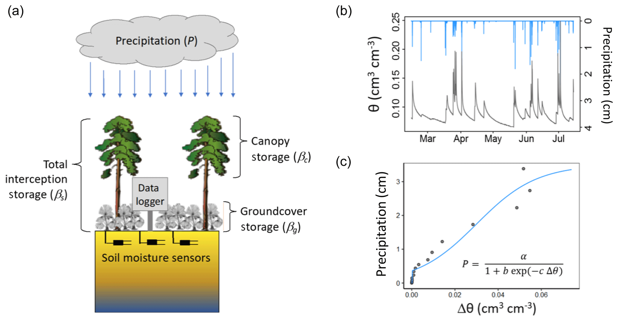
Figure 1(a) Schematic illustration of experimental setup and interception water storages, where total interception storage (βs) is the sum of canopy storage (βc) and groundcover (understory and litter) storage (βg). (b) Example time series of rainfall (blue lines) and corresponding near-surface soil moisture content (θ, black line; observed at 15 cm in this study). (c) Resultant relationship between rainfall and change in soil moisture Δθ during rainfall, along with a fitted model to extract the y intercept (i.e., Ps).

Figure 2Binned rainfall depths versus change in soil moisture content (Δθ) for six plots at one of the study sites used in the study (Econfina; EF). The y intercepts of the fitted relationships were used to derive Ps in Eq. (2). Note the different y-axis scale for EF Plot 3.
To estimate βs, we consider a population of individual rainfall events of varying depth over a forest for which high-frequency (i.e., 4 h−1) soil moisture measurements are available from near the soil surface. To ensure that canopy and groundcover layers are dry, and thus interception storage is zero prior to rainfall onset (i.e., antecedent interception storage capacity = βs), we further filter the rainfall data to only include the events that are separated by at least 72 h. Volumetric soil water content (θ) at the sensor changes only after rainfall fills βs, evaporative demands since rainfall onset are met, and there is sufficient infiltration for the wetting front to arrive at the sensor. Rainfall events large enough to induce a soil moisture change (Δθ) are evident as a rainfall threshold in the relationship between P and Δθ. An example time series of P and θ (Fig. 1b) yields a P versus Δθ relationship (Fig. 1c) with clear threshold behavior. There are multiple equations whose functional forms allow for extraction of this threshold; here we express this relationship as
where P is the total rainfall event depth, Δθ is the corresponding soil moisture change, and a, b, and c are fitted parameters. Figure 2 illustrates this relationship and model fitting for observed Δθ data from six plots at one of our study sites described below. We chose a reverse exponential function in Eq. (1) to fit the observed Δθ–P relationship because it aligns well with observations and is physically representative of the typical infiltration behavior observed across most soil profiles (e.g., Horton, 1941). While the data in Fig. 2 suggest that other functional forms (e.g., a linear equation with thresholds at Δθ=0 and Δθmax) could provide equivalent fidelity over the range of our observations, a constant slope would be inferior for describing the infiltration dynamics of the Δθ–P relationship more generally. The y intercept of Eq. (1) (i.e., where Δθ departs from zero) is given by
where Ps represents the total rainfall required to saturate βs, meet evaporative demands between storm onset and observed Δθ, and supply any infiltration required to induce soil moisture response once βs has been saturated. This equality can be expressed as
where T is the total time from rainfall onset until observed change in θ (i.e., the wetting-front arrival), t is the time when βs is satisfied, and E and f are the evaporation and infiltration rates, respectively. To connect this empirical observation to existing analytical frameworks (e.g., Gash, 1979), we adopt the term PG, defined as the rainfall depth needed to saturate βs and supply evaporative losses between rainfall onset (time = 0) and βs saturation (time = t):
Solving for βs in Eq. (3) and substituting into Eq. (4) yields
Equation (5) may be simplified by assuming that average infiltration and evaporation rates apply during the relatively short period between t and T, such that
where is the average soil infiltration rate and is the average rate of evaporation from the forest surface (i.e., canopy, ground cover, and soil) during the time from t to T (see Gash, 1979). The storage capacity βs can now be calculated following Gash (1979) as
where is the average rainfall rate and all other variables are as previously defined. In Eq. (5), is usually estimated using the Penman–Monteith equation (Monteith, 1965), setting canopy resistance to zero (e.g., Ghimire et al., 2017).
A key challenge in applying Eq. (5), and thus for the overall approach, is quantifying infiltration, since the time, t, when βs is satisfied is unknown. Moreover, the infiltration rate embedded in Ps is controlled by and initial soil moisture content (θi). It is worth noting that shallower sensor depth placement would likely eliminate the need for this step (see Discussion). However, to overcome this limitation in our study (where our soil moisture sensor was 15 cm below the ground surface), we used 1-D unsaturated flow model HYDRUS-1D (Vogel et al., 1995) to simulate the required time for the wetting front to arrive (Tw) at the sensor under bare soil conditions across many combinations of and θi. As such, Tw represents the time required for a soil moisture pulse to reach the sensor once infiltration begins (i.e., after βs has been filled), which is T−t in Eq. (7). For each simulation, Tw (signaled by the first change in θ at sensor depth) was recorded and used to develop a statistical model of Tw as a function of and θi. We used plot-specific soil moisture retention parameters from the Florida Soil Characterization Retrieval System (https://soils.ifas.ufl.edu/flsoils/, last access: 19 September 2019) to develop these curves for our sites, but simulations can be applied for any soil with known or estimated parameters.
Simulations revealed that Tw at a specific depth declined exponentially with increasing θi:
where a and b are fitting parameters. Moreover, the parameters a and b in Eq. (6) are well fitted by a power function of :
where a1 and b1 are fitting parameters. These relationships are illustrated in Fig. 3 for a loamy sand across a range of and θi at 15 cm depth. The relationship between θi and Tw is very strong for small to moderate (<3.0 cm h−1). At higher values of , Tw is smaller than the 15 min sampling resolution, and these events were excluded from our analysis (see below).
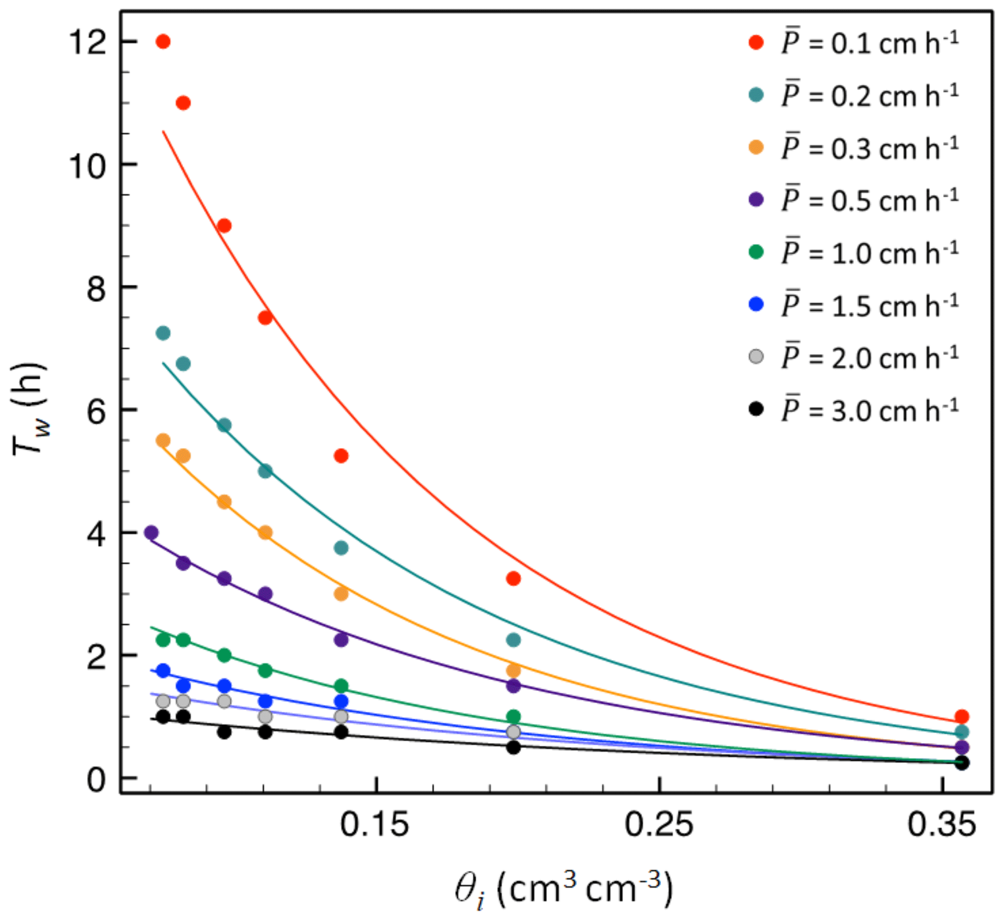
Figure 3Initial soil moisture content (θi) versus time of wetting-front arrival (Tw) at 15 cm depth for a loamy sand soil. Dots are simulated results from HYDUS-1D simulation, and lines are the exponential model given in Eq. (8), fitted for each rainfall rate, .
Assuming that equals over the initial infiltration period from t to T (robust for most soils; see below), Eq. (7) can be modified to
This approach assumes no surface runoff or lateral soil-water flow near the top of the soil profile from time t to T. Except for very fine soils under extremely high , this assumption generally holds during early storm phases, before ponding occurs (Mein and Larson, 1973). However, where strong layering occurs near the surface, lateral flow above the sensor (i.e., at capillary barriers or differential conductivity layers; Blume et al., 2009) may occur, and wetting-front simulations described above would need to account for layered soil structure to avoid potential overestimation of interception. Lateral flow within the duff layer during high-intensity precipitation events as observed by Blume et al. (2008) would be more difficult to correct for, though we note that since our goal is to determine βs, extreme storms can be omitted from the analysis when implementing Eqs. (1)–(10), without compromising βs estimates. Similarly, not accounting for the presence of preferential flow (e.g., finger flow, funnel flow, or macropore flow; Orozco-López et al., 2018) in wetting-front calculations could lead to underestimation of interception, though application in coarser texture soils (as evaluated here) likely minimizes this challenge. More generally, these limitations can be minimized by placing the soil moisture sensor close to the soil surface (e.g., within 5 cm). Finally, we note that values of βs from Eq. (10) represent combined interception from canopy and ground cover, but the method does not allow for disaggregation of these two components.
2.2 Calculating interception
Interception storage and subsequent evaporation (sometimes referred to as interception loss) for a given rain event are driven by both antecedent rain (which fills storage) and evaporation (which depletes it). Instantaneous available storage ranges from zero (saturated) to the maximum capacity (i.e., βs, which occurs when the storage is empty). While discrete, event-based interception models (Gash, 1979; Gash et al., 1995; Liu, 1997) have been widely applied to estimate interception, continuous models more accurately represent time-varying dynamics in interception storage and losses. We adopted the continuous, physically based interception modeling framework of Liu (1988, 1997, 2001):
where I is interception, D0 is the forest dryness index at the beginning of the time step t, D is the forest dryness index at the end of time t, and E is the evaporation rate from wetted surfaces. The dryness index at each time step is calculated as
where C is “adherent storage” (i.e., water that does not drip to the ground) and is given by
where τ is the free throughfall coefficient. Because our formulation of βs in Eq. (10) incorporates both canopy and groundcover components (i.e., negligible true throughfall), we approximated τ in Eq. (13) as zero. Between rainfall events, water in interception storage evaporates to meet atmospheric demand, until the dryness index, D, reaches unity (Liu, 1997). The rate of evaporation from wetted surfaces between rainfall events (Es) is
A numerical version of Eq. (11) to calculate interception at each time step, t, is expressed as
Equation (15) quantifies continuous and cumulative interception using precipitation and other climate data (for E) along with βs derived from soil moisture measurements and corresponding meteorological data.
2.3 Study area and data collection
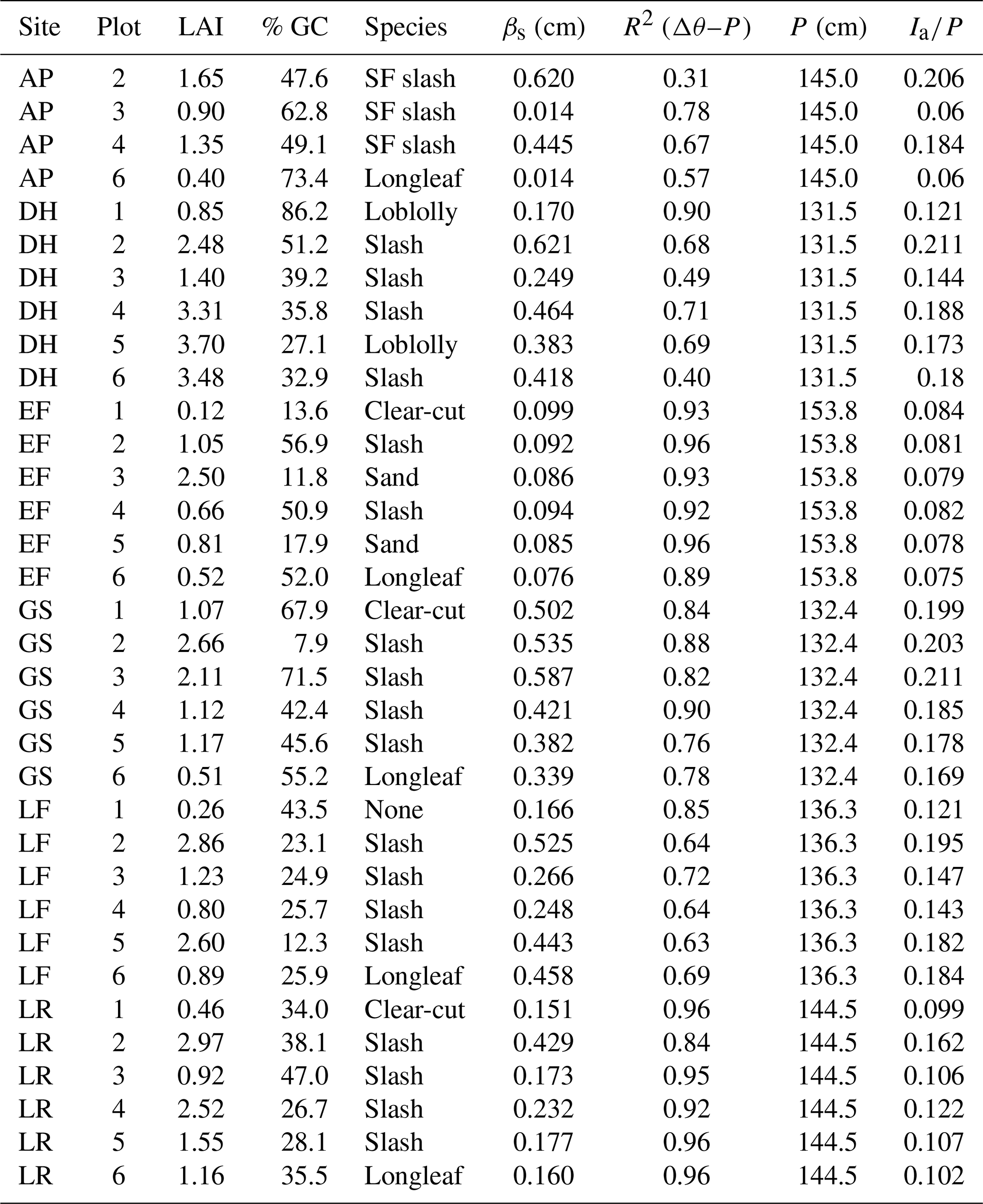
As part of a multi-year study quantifying forest water use under varying silvicultural management, we instrumented six sites across Florida, each with six 2 ha plots spanning a wide range of forest structural characteristics. Data from two of the plots at one site were not used here due to consistent surface water inundation, yielding a total of 34 experimental forest plots. Sites varied in hydroclimatic forcing (annual precipitation range: 131 to 154 cm yr−1 and potential ET range: 127 to 158 cm yr−1) and hydrogeologic setting (shallow versus deep groundwater table). Experimental plots within sites varied in tree species, age, density, leaf area index (LAI), groundcover vegetation density (% GC), soil type, and management history (Table 1). Each site contained a recent clear-cut plot, a mature pine plantation plot, and a restored longleaf pine (Pinus palustris) plot; the three remaining plots at each site included stands of slash pine (Pinus elliottii), sand pine (Pinus clausa), or loblolly pine (Pinus taeda) subjected to varying silvicultural treatments (understory management, canopy thinning, prescribed burning) and hardwood encroachment. The scope of the overall project (34 plots spanning six sites across Florida) and the emphasis on measuring variation in forest ET and water yield precluded conventional measurements of interception (e.g., throughfall and stemflow collectors). Because model estimates of interception were considered sufficient for water yield predictions across sites, the analyses presented here represent a proposal for additional insights about interception that can be gleaned from time series of soil moisture rather than a meticulous comparison of methods. We assessed results from this new proposed method by using comparisons with numerous previous interception studies in pine stands in the southeastern US and elsewhere and by testing for the expected associations between estimated interception and stand structure (e.g., LAI and ground cover).
Table 1Summary of storage capacity (βs) and annual interception losses (Ia) for all sites and plots, along with plot characteristics (mean annual precipitation, P; leaf area index, LAI; percent ground cover, % GC; and species). Note that the AP site only had four plots with the data required for the analysis.
Within each plot, three sets of TDR sensors (CS655, Campbell Scientific, Logan, UT, USA) were installed to measure soil moisture at multiple soil depths (Fig. 1a). Only data from the top-most sensor (15 cm below the ground surface) were used in this study. Soil moisture sensors were located to capture representative variation in stand geometry and structure (i.e., within and between tree rows) to capture variation in surface soil moisture response to rainfall events. While this spatial layout was intended to characterize the range of plot-scale forest canopy and groundcover heterogeneity, the three measurement locations were within a 10 m radius and thus represent localized (sub-plot) interception estimates. Within each clear-cut plot at each site, meteorological data (rainfall, air temperature, relative humidity, solar insolation, wind speed, and direction) were measured using a weather station (GRSW100, Campbell Scientific, Logan, UT; Fig. 4c) every 3 s and used to calculate hourly E by setting the canopy resistance to zero (Ghimire et al., 2017; Gash et al., 1995; Monteith, 1965). Growing season forest canopy LAI (m2 m−2) and ground cover (%) were measured at every 5 m node within a 50 m × 50 m grid surrounding soil moisture measurement banks. LAI was measured at a height of 1 m using a LI-COR LAI-2200 plant canopy analyzer, and % GC was measured using a 1 m2 quadrat.
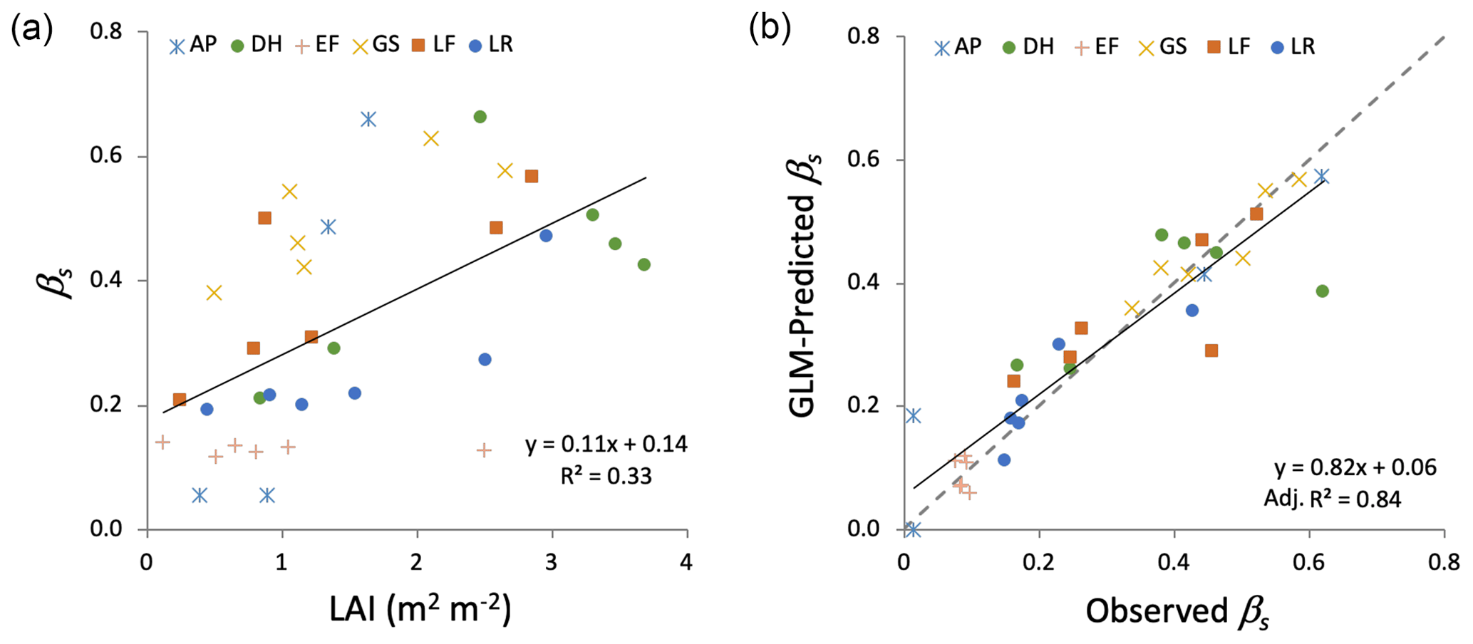
Figure 4(a) Interception storage capacity (βs) versus leaf area index (LAI) for all sites and plots. (b) Modeled versus observed βs using the best GLM, which included % GC vegetation and an interaction term between site and LAI. The dashed line is the 1:1 line.
To estimate βs, mean Δθ values from the three surface sensors were calculated for all rainfall events separated by at least 72 h. Storm separation was necessary to ensure the canopy and groundcover surfaces were mostly dry (and thus antecedent storage capacity = βs) at the onset of each included rainfall event. Rainfall events were binned into discrete classes by depth and plotted against mean Δθ to empirically estimate Ps (e.g., Fig. 2). For each rainfall bin, mean θi, , and were also calculated to use in Eq. (10), which was then applied to calculate βs. Subsequently, we developed generalized linear models (GLMs) using forest canopy structure (site-mean LAI), mean ground cover (% GC), hydrogeologic setting (shallow versus deep groundwater table), and site as potential predictors, along with their interactions, to statistically assess predictors of βs estimates. Because models differed in fitted parameter number, the best model was selected using the Akaike information criterion (AIC; Akaike, 1974). Finally, we calculated cumulative annual interception (Ia) and its proportion of total precipitation (Ia∕P) for each study plot using the mean βs for each plot (across the three sensor banks), climate data from 2014 to 2016, and Eq. (15). Differences in Ia∕P across sites and among plots within sites were assessed using ANOVAs. All analyses were performed using R (R Core Team, 2017).
3.1 Total storage capacity (βs)
The exponential function used to describe the P–Δθ relationship (Eq. 1) showed strong agreement with observations at all sites and plots (overall R2=0.80; ; Table 1) as illustrated for a single site in Fig. 2. This consistency across plots and sites suggests that Eq. (1) is capable of adequately describing observed P–Δθ relationships, enabling estimates of βs across diverse hydroclimatic settings and forest structural variation. Estimates of βs ranged from 0.01 to 0.62 cm, with a mean of 0.30 cm (Table 1). Plot-scale LAI was moderately correlated with plot-mean βs, describing roughly 32 % of observed variation across plots (Fig. 4a). This relatively weak association may arise because LAI measurements only characterize canopy cover, while βs combines canopy and groundcover storage. The best GLM of βs (Fig. 4b) used % GC and an interaction term between site and LAI (R2=0.84 and AIC = 253.7, Table 2). The best GLM without site used LAI and hydrogeologic setting (shallow versus deep water table) but had reduced performance (R2=0.55 and AIC = 338.3; Table 2). All models excluding LAI as a predictor performed poorly, so we report model comparisons only for those including LAI.
Table 2Summary of generalized linear model (GLM) results for interception storage capacity (βs). LAI is leaf area index, GC is ground cover, and WT is water table (shallow versus deep). The best model needs to be noted in BOLD (Model no. 4).

3.2 Annual interception (Ia)
Despite having similar rainfall regimes (mean annual precipitation ranging from 131 to 154 cm yr−1 across sites), mean annual interception (Ia) differed significantly both across sites (one-way ANOVA p<0.001) and among plots within sites (one-way ANOVA p<0.001). Estimates of Ia∕P across all plots and sites ranged from 6 % to 21 % of annual rainfall (Table 1) and were moderately, but significantly, correlated with mean LAI, explaining approximately 30 % of variation in Ia∕P (Fig. 5a). Correlations among Ia∕P and LAI were stronger for individual sites than the global relationship (), except for site EF, where Ia was small and similar across plots regardless of LAI (Fig. 5b; Table 1). This suggests that additional site-level differences (e.g., hydroclimate, soils, geology) play a role in driving Ia, as expected following from their effects on βs described above.
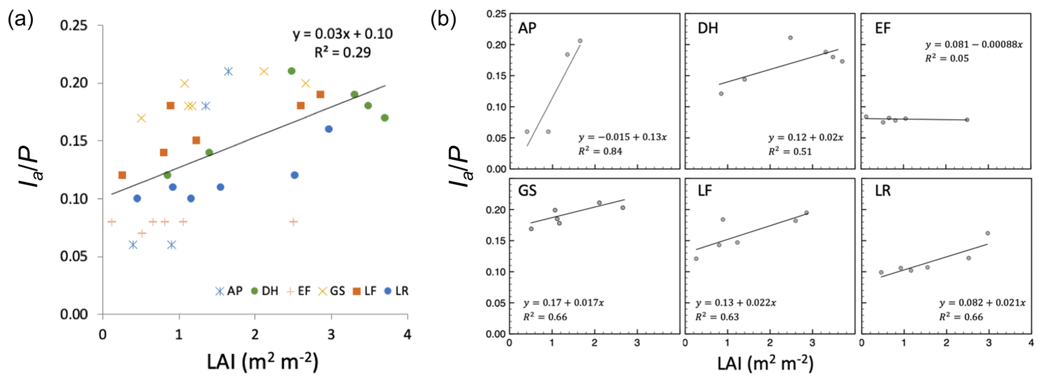
Figure 5(a) Annual proportion of rainfall that is intercepted (Ia∕P) versus LAI for all sites and plots. (b) Site-specific Ia∕P versus LAI relationships. The relationship is generally strong except for the EF site, where the overall storage capacity is small across all values of LAI.
When combined with local rainfall data, near-surface soil moisture dynamics inherently contain information about rainfall interception by above-ground structures. Using soil moisture data, we developed and tested an analytical approach for estimating total interception storage capacity (βs) that includes canopy, understory, and groundcover vegetation, as well as any litter on the forest floor. The range of βs given by our analysis (mean βs=0.30 cm; cm) is close to but generally higher than previously reported canopy-only storage capacity values for similar pine forests (e.g., 0.17 to 0.20 cm for mature southeastern USA pine forests; Bryant et al., 2005). Moreover, our estimates of βs and annual interception corresponded to expected forest structure controls (e.g., LAI and ground cover) on interception, further supporting the feasibility of the soil moisture-based approach. However, we emphasize that a more robust validation of the method using co-located and contemporaneous measurement using standard techniques is warranted. Below we summarize the assumptions and methodological considerations that affect the potential utility and limitation of the method.
An important distinction between our proposed method and previous interception measurement approaches is that the soil moisture-based method estimates composite rainfall interception of not only the canopy, but also of the groundcover vegetation and forest floor litter. Rainfall storage and subsequent evaporation from groundcover vegetation and litter layers can be as high as, or higher than, canopy storage in many forest landscapes (Putuhena and Cordery, 1996; Gerrits et al., 2010). For example, Li et al. (2017) found that the storage capacity of a pine forest floor in China was between 0.3 and 0.5 cm, while maximum canopy storage was <0.1 cm. Putuhena and Cordery (1996) also estimated the storage capacity of pine forest litter to be approximately 0.3 cm based on direct field measurements. Gerrits et al. (2007) found forest floor interception to be 34 % of measured precipitation in a beech forest, while other studies have shown that interception by litter can range from 8 % to 18 % of total rainfall (Gerrits et al., 2010; Tsiko et al., 2012; Miller et al., 1990; Pathak et al., 1985; Kelliher et al., 1992). A recent study using leaf wetness observations (Acharya et al., 2017) found the storage capacity of eastern red-cedar (Juniperus virginiana) forest litter to range from 0.12 to as high as 1.12 cm, with forest litter intercepting approximately 8 % of gross rainfall over a 6-month period. Given the composite nature of forest interception storage and the range of storage capacities reported in these studies, the values we report appear to be plausible and consistent with the expected differences between canopy-only and total interception storage.
Interception varies spatially and temporally and is driven by both βs and climatic variation (i.e., P and E). Our approach represents storage dynamics by combining empirically derived βs estimates with climatic data using a previously developed continuous interception model (Liu, 1997, 2001). Cumulative Ia estimates in this study ranged considerably (i.e., from 6 % to 21 % of annual rainfall) across the 34 plots, which were characterized by variation in canopy structure (0.12 < LAI < 3.70) and ground cover (7.9 < % GC < 86.2). In comparison, interception by pine forests reported in the literature (all of which report either canopy-only or groundcover-only values, but not their composite) range from 12 % to 49 % of incoming rainfall (Bryant et al., 2005; Llorens and Poch, 1997; Kelliher et al., 1992; Crockford and Richardson, 2000). Notably, most of the variation in this range is driven by climate rather than forest structure, with the highest Ia values from more arid regions (e.g., Llorens and Poch, 1997). Future work could also consider seasonally disaggregated measurements to explore intra-annual variation in canopy structure and litter composition (Van Stan et al., 2017).
Broad agreement between our results and literature Ia values again supports the potential utility of our method for estimating this difficult-to-measure component of the water budget, though additional direct comparisons would further support this assertion. Additionally, the magnitude and heterogeneity of our Ia estimates across a single forest type (southeastern US pine) underscore the urgent need for empirical measurements of interception that incorporate information on both canopy and groundcover storage in order to develop accurate water budgets. This conclusion is further bolstered by the persistent importance of site-level statistical effects in predicting βs (and therefore Ia), even after accounting for forest structural attributes, which suggests there are influential edaphic or structural attributes that we are not currently adequately assessing. For example, while estimated Ia in clear-cut plots was generally smaller than plots with a developed canopy, as expected, one exception was at EF, where the clear-cut plot exhibited the highest Ia of the six EF plots (8.4 %, Table 1). However, differences among all EF plots were very small (Ia ranged only from 7.9 % to 8.4 % of annual rainfall), a rate consistent with or even lower than other clear cuts across the study. This site is extremely well drained with nutrient-poor sandy soils and differs from other sites in that it has dense litter dominated by mosses, highlighting the need for additional local measurements to better understand how forest structure controls observed interception.
There are several important methodological considerations and assumptions inherent to estimating interception using near-surface soil moisture data. First is the depth at which soil moisture is measured. Ideally, θ would be measured a few centimeters into the soil profile, eliminating the need to account for infiltration when calculating PG in Eqs. (4)–(6) and thereby alleviating concerns about lateral and preferential flow. Soil moisture data used here were leveraged from a study of forest water yield, with sensor deployment depths selected to efficiently integrate soil moisture patterns through the vadose zone. The extra step of modeling infiltration likely increases uncertainty in βs given field-scale heterogeneity in soil properties and potential lateral and preferential flow. Specifically, lateral flow would delay wetting-front arrival, leading to overestimation of interception, while preferential flow would do the opposite. Despite these caveats, infiltration in our system was extremely well described using wetting-front simulations of arrival time based on initial soil moisture and rainfall. As such, while we advocate for shallower sensor installation and direct comparison to standard methods in future efforts, the results presented here given the available sensor depth seem tenable for this and other similar data sets.
Another methodological consideration is that, in contrast to the original Gash (1979) formulation, Eq. (5) does not explicitly include throughfall. While throughfall has been a critical consideration for rainfall partitioning by the forest canopy, our approach considers total interception by above-ground forest structures (canopy, ground cover, and litter). A portion of canopy throughfall is captured by non-canopy storage and is thus intercepted. Constraining this fraction is not possible with the data available, and indeed our soil moisture response reflects the “throughfall” passing the canopy, understory, and litter. Similarly, estimation of βs using Eqs. (1)–(7) cannot directly account for stemflow, which can be an important component of rainfall partitioning in forests (e.g., Bryant et al., 2005). We used the mean soil moisture response across three sensor locations (close to a tree, away from the tree but below the canopy, and within inter-canopy rows), which lessens the impact of this assumption on our estimates of βs. Further, Eqs. (3)–(10) assume the same evaporation rate, E, for intercepted water from the canopy and from the understory. Evaporation rates may vary substantially between the canopy, understory, and forest floor (Gerrits et al., 2007, 2010), especially in more energy-limited environments. Future work should consider differential evaporation rates within each interception storage, particularly since the inclusion of litter as a component potentially accentuates these contrasts in E.
Among the many challenges of measuring interception is the spatial heterogeneity of canopy and groundcover layers, with associated heterogeneity in interception rates. Our study deployed only three sensors per plot, yielding interception estimates that covaried with the expected forest structure controls (i.e., LAI and ground cover) and that aligned closely with literature-reported values. Nonetheless, future work should assess spatial variation in soil moisture responses to known heterogeneity in net precipitation (i.e., throughfall plus stemflow) across forest stands (e.g., Roth et al., 2007; Wullaert et al., 2009; Fathizadeh et al., 2014). Soil moisture responses are likely driven by variation in both vegetation and soil properties (Metzger et al., 2017), indicating the need for future inquiry across systems to inform the number and locations of soil moisture sensors needed for accurate interception estimates in a variety of settings. Notably, the requisite sampling frequency for above-ground interception is estimated to be 25 funnel collectors per hectare (or more) to maintain relative error below 10 % for long-term monitoring, with as many as 200 collectors needed for similar error rates during individual event sampling (Zimmerman et al., 2010; Zimmerman and Zimmerman, 2014). Spatial averaging using larger trough collectors reduces some of this sampling effort, yielding guidance of 5 trough collectors per hectare for assessment of multiple precipitation events or up to 20 per hectare for individual events (Zimmerman and Zimmerman, 2014).
While the comparative spatial integration extent of above-ground collectors versus soil moisture sensors remains unknown, the strong correspondence between our measurements and literature-reported values for the magnitude of interception storage, as well as the forest structure controls (i.e., LAI and ground cover) on that storage volume, underscores that soil moisture measurements, at least in this setting, can integrate key quantitative aspects of the interception process. One possible explanation for the consistency of our results with previous interception studies using above-ground collectors is that soil moisture averages across extant spatial heterogeneity in canopy processes, providing comparable spatial integration to throughfall troughs. In this context, soil moisture measurements have several operational advantages over trough-type collectors, including automated data logging and reduced maintenance burden (e.g., clearing litter accumulation in collectors), while also providing total interception estimates (as opposed to canopy-only measures). Additional soil moisture measurements would undoubtedly improve the accuracy of these estimates, and indeed we recommend that more direct methodological comparisons are needed to determine the optimal number of sensors for future applications. Overall, however, our results support the general applicability of this proposed soil moisture-based approach for developing “whole-forest” interception estimates across a wide range of hydroclimatic and forest structural settings.
Rainfall interception by forests is a dynamic process that is strongly influenced by rainfall patterns (e.g., frequency, intensity), along with various forest structural attributes such as interception storage capacity (βs) (Gerrits et al., 2010). In this work, we coupled estimation of a total (or “whole-forest”) βs parameter with a continuous water balance model (Liu, 1997, 2001; Rutter et al., 1975), providing an integrative approach for quantifying time-varying and cumulative interception. We propose that soil moisture-based estimates of βs have the potential to more easily and appropriately represent combined forest interception relative to existing time- and labor-intensive field methods that fail to account for groundcover and litter interception. However, we emphasize that further experimental work is needed to validate this promising approach. Soil moisture can be measured relatively inexpensively and easily using continuous logging sensors that require little field maintenance, facilitating application of the presented approach across large spatial and temporal extents and reducing the time and resources that are needed for other empirical measures (e.g., Lundberg et al., 1997). Finally, while our comparisons with other empirical measures of forest canopy interception should be treated cautiously, this approach yields values that are broadly consistent with the literature and provide an estimate of combined canopy and groundcover storage capacity that has the potential to improve the accuracy of water balance models at scales from the soil column to watershed.
All data and associated metadata are available on the Consortium of Universities for the Advancement of Hydrologic Science (CUAHSI) HydroShare portal: http://www.hydroshare.org/resource/50620fac707c400cbdcf7392a1b895cf (last access: 9 April 2020) (Cohen, 2020).
SA performed the primary analysis and developed the first draft of the manuscript; DM, DK, and MC contributed equally to additional analysis and manuscript development.
The authors declare that they have no conflict of interest.
We are grateful for project oversight by Bill Bartnick (FDACS), site access and project management from Stephen Miller and Jeremy Olson (SJRWMD), Bob Heeke (SRWMD), Bill Cleckley (NWFWMD), Sean King and Allan Milligan (SWFWMD), and Jeff Sumner and Eva Mendez (SFWMD). Field support from Kenyon Watkins, Brett Caudill, Paul Decker, Kevin Henson, and Larry Kohrnak was instrumental in producing the dataset used in this analysis.
This research has been supported by the Florida Department of Agricultural and Consumer Services and the Northwest Florida Water Management District (NWFWMD), the South Florida Water Management District (SFWMD), the Southwest Florida Water Management District (SWFWMD), the St. Johns River Water Management District (SJRWMD), and the Suwannee River Water Management District (SRWMD).
This paper was edited by Miriam Coenders-Gerrits and reviewed by John Van Stan and one anonymous referee.
Acharya, B. S., Stebler, E., and Zou, C. B.: Monitoring litter interception of rainfall using leaf wetness sensor under controlled and field conditions, Hydrol. Process., 31, 240–249, https://doi.org/10.1002/hyp.11047, 2005.
Akaike, H.: A new look at the statistical model identification, IEEE T. Automat. Control, 19, 716–723, 1974.
Blume, T., Zehe, E., and Bronstert, A.: Investigation of runoff generation in a pristine, poorly gauged catchment in the Chilean Andes. II: Qualitative and quantitative use of tracers at three different spatial scales, Hydrol. Process., 22, 3676–3688, 2008.
Blume, T., Zehe, E., and Bronstert, A.: Use of soil moisture dynamics and patterns at different spatio-temporal scales for the investigation of subsurface flow processes, Hydrol. Earth Syst. Sci., 13, 1215–1233, https://doi.org/10.5194/hess-13-1215-2009, 2009.
Bryant, M. L., Bhat, S., and Jacobs, J. M.: Measurements and modeling of throughfall variability for five forest communities in the southeastern US, J. Hydrol., 312, 95–108, https://doi.org/10.1016/j.jhydrol.2005.02.012, 2005.
Calder, I. R.: A stochastic model of rainfall interception, J. Hydrol., 89, 65–71, https://doi.org/10.1016/0022-1694(86)90143-5, 1986.
Calder, I. R.: Evaporation in the Uplands, Wiley, New York, 148 pp., 1990.
Cohen, M.: Measurements of Forest Interception using Near Surface Soil Moisture Responses, HydroShare, available at: http://www.hydroshare.org/resource/50620fac707c400cbdcf7392a1b895cf, last access: 9 April 2020.
Crockford, R. H. and Richardson, D. P.: Partitioning of rainfall into throughfall, stemflow and interception: effect of forest type, ground cover and climate, Hydrol. Process., 14, 2903–2920, https://doi.org/10.1002/1099-1085(200011/12)14:16/17<2903::AID-HYP126>3.0.CO;2-6, 2000.
David, T. S., Gash, J. H. C., Valente, F., Pereira, J. S., Ferreira, M. I., and David, J. S.: Rainfall interception by an isolated evergreen oak tree in aMediterranean savannah, Hydrol. Process., 20, 2713–2726, https://doi.org/10.1002/hyp.6062, 2006.
Fathizadeh, O., Attarod, P., Keim, R. F., Stein, A., Amiri, G. Z., and Darvishsefat, A. A.: Spatial heterogeneity and temporal stability of throughfall under individual Quercus brantii trees, Hydrol. Process., 28, 1124–1136, 2014.
Gash, J. H. C.: An analytical model of rainfall interception by forests, Q. J. Roy. Meteorol. Soc., 105, 43–55, https://doi.org/10.1002/qj.49710544304, 1979.
Gash, J. H. C., Lloyd, C. R., and Lachaud, B. G.: Estimating sparse forest rainfall interception with an analytical model, J. Hydrol., 170, 79–86, 1995.
Gerrits, A. M. J. and Savenije, H. H. G.: Forest floor interception, in: Forest hydrology and biogeochemistry, Springer, Dordrecht, 445–454, 2011.
Gerrits, A. M. J., Savenije, H. H. G., Hoffmann, L., and Pfister, L.: New technique to measure forest floor interception – an application in a beech forest in Luxembourg, Hydrol. Earth Syst. Sci., 11, 695–701, https://doi.org/10.5194/hess-11-695-2007, 2007.
Gerrits, A. M. J., Pfister, L., and Savenije, H. H. G.: Spatial and temporal variability of canopy and forest floor interception in a beech forest, Hydrol. Process., 24, 3011–3025, 2010.
Ghimire, C. P., Bruijnzeel, L. A., Lubczynski, M. W., and Bonell, M.: Rainfall interception by natural and planted forests in the Middle Mountains of Central Nepal, J. Hydrol., 475, 270–280, https://doi.org/10.1016/j.jhydrol.2012.09.051, 2012.
Ghimire, C. P., Bruijnzell, L. A., Lubczynski, M. W., Ravelona, M., Zwartendijk, B. W., and Meervald, H. H.: Measurement and modeling of rainfall interception by two differently aged secondary forests in upland eastern Madagascar, J. Hydrol., 545, 212–225, https://doi.org/10.1016/j.jhydrol.2016.10.032, 2017.
Guevara-Escobar, A., González-Sosa, E., Véliz-Chávez, C., Ventura-Ramos, E. and Ramos-Salinas, M.: Rainfall interception and distribution patterns of gross precipitation around an isolated Ficus benjamina tree in an urban area, J. Hydrol., 333, 532–541, 2007.
Horton, R. E.: An approach toward a physical interpretation of infiltration-capacity 1, Soil Sci. Soc. Am. J., 5, 399–417, 1941.
Kelliher, F. M., Whitehead, D., and Pollock, D. S.: Rainfall interception by trees and slash in a young Pinus radiata D. Don stand, J. Hydrol., 131, 187–204, https://doi.org/10.1016/0022-1694(92)90217-J, 1992.
Li, X., Xiao, Q., Niu, J., Dymond, S., Mcherson, E. G., van Doorn, N., Yu, X., Xie, B., Zhang, K., and Li, J.: Rainfall interception by tree crown and leaf litter: an interactive process, Hydrol. Process., 31, 3533–3542, https://doi.org/10.1002/hyp.11275, 2017.
Liu, J.: A theoretical model of the process of rainfall interception in forest canopy, Ecol. Model., 42, 111–123, 1988.
Liu, S.: A new model for the prediction of rainfall interception in forest canopies, Ecol. Model., 99, 151–159, 1997.
Liu, S.: Estimation of rainfall storage capacity in the canopies of cypress wetlands and slash pine uplands in North-Central Florida, J. Hydrol., 207, 32–41, 1998.
Liu, S.: Evaluation of the Liu model for predicting rainfall interception in forests world‐wide, Hydrol. Process., 15, 2341–2360, 2001.
Llorens, P. and Poch, R.: Rainfall interception by a Pinus sylvestris forest patch overgrown in a Mediterranean mountainous abandoned area I. Monitoring design and results down to the event scale, J. Hydrol., 199, 331–345, 1997.
Lundberg, A., Eriksson, M., Halldin, S., Kellner, E., and Seibert, J.: New approach to the measurement of interception evaporation, J. Atmos. Ocean. Tech., 14, 1023–1035, 1997.
Mein, R. G. and Larson, C. L.: Modeling infiltration during a steady rain, Water Resour. Res., 9, 384–394, 1973.
Merriam, R. A.: A note on the interception loss equation, J. Geophys. Res., 65, 3850–3851, https://doi.org/10.1029/JZ065i011p03850, 1960.
Metzger, J. C., Wutzler, T., Dalla Valle, N., Filipzik, J., Grauer, C., Lehmann, R., Roggenbuck, M., Schelhorn, D., Weckmüller, J., Küsel, K., and Totsche, K. U.: Vegetation impacts soil water content patterns by shaping canopy water fluxes and soil properties, Hydrol. Process., 31, 3783–3795, 2017.
Miller, J. D., Anderson, H. A., Ferrier, R. C., and Walker, T. A. B.: Comparison of the hydrological budgets and detailed hydrological responses in two forested catchments, Forestry, 63, 251–269, 1990.
Monteith, J. L.: Evaporation and environment, in: Symposia of the society for experimental biology, Vol. 19, Cambridge University Press (CUP), Cambridge, 205–234, 1965.
Muzylo, A., Llorens, P., Valente, F., Keizer, J. J., Domingo, F., and Gash, J. H. C.: A review of rainfall interception modelling, J. Hydrol., 370, 191–206, https://doi.org/10.1016/j.jhydrol.2009.02.058, 2009.
Orozco-López, E., Muñoz-Carpena, R., Gao, B., and Fox, G. A.: Riparian vadose zone preferential flow: Review of concepts, limitations, and perspectives, Vadose Zone J., 17, 180031, https://doi.org/10.2136/vzj2018.02.0031, 2018.
Pathak, P. C., Pandey, A. N., and Singh, J. S.: Apportionment of rainfall in central Himalayan forests (India), J. Hydrol., 76, 319–332, 1985.
Putuhena, W. M. and Cordery, I.: Estimation of interception capacity of the forest floor, J. Hydrol., 180, 283–299, 1996.
R Core Team: R: A language and environment for statistical computing, page R Foundation for Statistical Computing, R Found. Stat. Comput., Vienna, Austria, available at: http://www.R-project.org/ (last access: 9 April 2020), 2017.
Roth, B. E., Slatton, K. C., and Cohen, M. J.: On the potential for high-resolution lidar to improve rainfall interception estimates in forest ecosystems, Front. Ecol. Environ., 5, 421–428, 2007.
Rutter, A. J., Kershaw, K. A., Robins, P. C., and Morton, A. J.: A predictive model of rainfall interception in forests, 1. Derivation of the model from observations in a plantation of Corsican pine, Agr. Meteorol., 9, 367–384, 1971.
Rutter, A. J., Morton, A. J., and Robins, P. C.: A Predictive Model of Rainfall Interception in Forests. II. Generalization of the Model and Comparison with Observations in Some Coniferous and Hardwood Stands, J. Appl. Ecol., 12, 367–380, 1975.
Savenije, H. H. G.: The importance of interception and why we should delete the term evapotranspiration from our vocabulary, Hydrol. Process., 18, 1507–1511, 2004.
Tsiko, C. T., Makurira, H., Gerrits, A. M. J., and Savenije, H. H. G.: Measuring forest floor and canopy interception in a savannah ecosystem, Phys. Chem. Earth Pt. A/B/C, 47, 122–127, 2012.
Van Stan, J. T., Coenders-Gerrits, M., Dibble, M., Bogeholz, P., and Norman, Z.: Effects of phenology and meteorological disturbance on litter rainfall interception for a Pinus elliottii stand in the Southeastern United States, Hydrol. Process., 31, 3719–3728, 2017.
Vogel, T., Huang, K., Zhang, R., and van Genuchten, M. T.: The HYDRUS (Version 5.0) code for simulating one-dimensional water flow, solute transport, and heat movement in variably-saturated media, Res. Rep. 135, US Salinity Laboratory, USDA, ARS Riverside, CA, 1995.
Wei, Z., Yoshimura, K., Wang, L., Miralles, D. G., Jasechko, S., and Lee, X.: Revisiting the contribution of transpiration to global terrestrial evapotranspiration, Geophys. Res. Lett., 44, 2792–2801, https://doi.org/10.1002/2016GL072235, 2017.
Wullaert, H., Pohlert, T., Boy, J., Valarezo, C., and Wilcke, W.: Spatial throughfall heterogeneity in a montane rain forest in Ecuador: extent, temporal stability and drivers, J. Hydrol., 377, 71–79, 2009.
Zimmermann, A. and Zimmermann, B.: Requirements for throughfall monitoring: The roles of temporal scale and canopy complexity, Agr. Forest Meteorol., 189, 125–139, 2014.
Zimmermann, B., Zimmermann, A., Lark, R. M., and Elsenbeer, H.: Sampling procedures for throughfall monitoring: a simulation study, Water Resour. Res., 46, W01503, https://doi.org/10.1029/2009WR007776, 2010.