Evaluation of soil moisture from CCAM-CABLE simulation, satellite-based models estimates and satellite observations: a case study of Skukuza and Malopeni flux towers

Reliable estimates of daily, monthly and seasonal soil moisture are useful in a variety of disciplines. The availability of continuous in situ soil moisture observations in southern Africa barely exists; hence, process-based simulation model outputs are a valuable source of climate information, needed for guiding farming practices and policy interventions at various spatio-temporal scales. The aim of this study is to evaluate soil moisture outputs from simulated and satellite-based soil moisture products, and to compare modelled soil moisture across different landscapes. The simulation model consists of a global circulation model known as the conformal-cubic atmospheric model (CCAM), coupled with the CSIRO Atmosphere Biosphere Land Exchange model (CABLE). The satellite-based soil moisture data products include satellite observations from the European Space Agency (ESA) and satellite-observation-based model estimates from the Global Land Evaporation Amsterdam Model (GLEAM). The evaluation is done for both the surface (0–10 cm) and root zone (10–100 cm) using in situ soil moisture measurements collected from two study sites. The results indicate that both the simulation- and satellite-derived models produce outputs that are higher in magnitude range compared to in situ soil moisture observations at the two study sites, especially at the surface. The correlation coefficient ranges from 0.7 to 0.8 (at the root zone) and 0.7 to 0.9 (at the surface), suggesting that models mostly are in an acceptable phase agreement at the surface than at the root zone, and this was further confirmed by the root mean squared error and the standard deviation values. The models mostly show a bias towards overestimation of the observed soil moisture at both the surface and root zone, with the CCAM-CABLE showing the least bias. An analysis evaluating phase agreement using the cross-wavelet analysis has shown that, despite the models' outputs being in phase with the in situ observations, there are time lags in some instances. An analysis of soil moisture mutual information (MI) between CCAM-CABLE and the GLEAM models has successfully revealed that both the simulation and model estimates have a high MI at the root zone as opposed to the surface. The MI mostly ranges between 0.5 and 1.5 at both the surface and root zone. The MI is predominantly high for low-lying relative to high-lying areas.

1 Introduction

Accurate estimates¹ of daily, monthly and seasonal soil moisture are important in a number of fields including agriculture (McNally et al., 2016); water resources planning (Decker, 2015); weather forecasting (van den Hurk et al., 2012); and the quantification of the impacts of extreme weather events such as droughts (Sheffield and Wood, 2008), heat waves (Fischer et al., 2007; Lorenz et al., 2010) and floods (Brocca et al., 2011). Soil moisture has been identified as one of the 50 essential climate variables (ECVs) by the Global Climate Observing System (GCOS) and the European Space Agency climate change initiative (ESA-CCI) (McNally et al., 2016). Available soil moisture affects the fluxes of heat and water at the surface and directly impacts local and regional weather patterns (Dorigo et al., 2015; Raoult et al., 2018; Yuan and Quiring, 2017).

Soil moisture is a key parameter to consider in the partitioning of precipitation and net radiation. The temporal and spatial variation in soil moisture is controlled by vegetation, topography, soil properties and climate variability (Xia et al., 2015). Root-zone soil moisture plays a vital role in the transpiration process of evapotranspiration (ET), especially in arid and semi-arid regions, where most of the water loss is accounted for by transpiration during the dry period (Jovanovic et al., 2015; Palmer et al., 2015). The dry period, which constitutes months when the sites experience minimum rainfall, occurs during the austral winter season, May to October. Regions where soil moisture strongly influences the atmosphere are at the transition between wet and dry climates. This is associated with the strong coupling between ET and soil moisture, which is a characteristic of these regions (van den Hurk et al., 2012; Lorenz et al., 2010).

The model evaluation in this study is achieved through a qualitative and quantitative comparison of modelled and in situ soil moisture products. Modelled and satellite-data-derived soil moisture fields are at different temporal and spatial resolutions while in site observations are mainly point-based (Fang et al., 2016). Despite the in situ data being limited in coverage, they are very useful for the calibration and validation of modelled and satellite-derived soil moisture estimates (Xia et al., 2015). Point-based in situ soil moisture data that are used as a reference in this study consist of surface and root-zone measurements. The fact that the in situ data are point-based poses significant challenges in the understanding of spatial patterns in soil moisture (Yuan and Quiring, 2017). Direct satellite observations, on the other hand, are presently only available for the surface. To obtain root-zone estimates of soil moisture, satellite-based surface soil moisture data are used in conjunction with ground-based observations and model estimates. The modelled soil moisture data are largely dependent on accurate surface forcing data (e.g. air temperature, precipitation and radiation) and the parameterization of the land surface schemes (Xia et al., 2015). This is done in the framework of physically based models whose accuracy may vary depending on the response of the models to the forcing data.

The study is inspired by the notion that an understanding of soil moisture characteristic patterns for the study region can be reliably obtained by looking at independent datasets from simulation experiments, theoretical or analytical models, and in situ observations. In Africa, the evaluations of the soil moisture data products, from these various estimation approaches, are sparse mainly due to the lack of publicly available in situ observations (Sinclair and Pegram, 2010). The lack of publicly available long-term and complete in situ soil moisture measurements in most parts of the world leads to a reliance on global climate models (GCMs) to estimate the land surface states (Dirmeyer et al., 2013). The data produced by land surface models, hydrological models and GCMs have been widely evaluated for many continents and regions (Albergel et al., 2012; An et al., 2016; Dorigo et al., 2015; McNally et al., 2016; Yuan and Quiring, 2017). The available studies include those conducted by McNally et al. (2016) and Dorigo et al. (2015), who evaluated ESA-CCI satellite soil moisture products over East and West Africa respectively.

The aims of this study are twofold. The first is to evaluate the ability of the process-based simulation and satellite-derived soil moisture products to capture the observed variability in soil moisture at specific flux tower locations. The second is to understand how the simulated results of soil moisture from a coupled land–atmosphere model compare against satellite-based estimates on broad landscape classes that belong to homogenous elevation and soil types. The evaluation is undertaken at two soil depths, namely surface (SSM, i.e. 0–10 cm) and root zone (RZSM, i.e. 10–100 cm), using long-term in situ measurements to determine whether the respective soil moisture data products are representative of local conditions. This is done for two study sites whose data records are available on request from the Council for Scientific and Industrial Research (CSIR) and FLUXNET, namely the Skukuza and Malopeni flux tower sites located in the Kruger National Park in South Africa. The two study sites receive summer rainfall and the colder winter months overlap with the dry period. Of these two sites, only the Skukuza site forms part of the global flux data network (FLUXNET). Other international flux observation networks, such as the International Soil Moisture Network (ISMN), have no affiliated data sites in the study region.

We investigate how the CCAM-CABLE process-based simulation, satellite-derived and GLEAM estimates compare with the in situ observations. We look at the spatio-temporal variations in simulated soil moisture data from a coupled land–atmosphere model. The conformal cubic atmospheric model (CCAM) of the Commonwealth Scientific and Industrial Research Organisation (CSIRO) coupled to the CSIRO Atmosphere Biosphere Land Exchange (CABLE) model, three versions of the European Space Agency (ESA) satellite observations (i.e. active, passive and combined), and estimates from three versions of the global land evaporation Amsterdam Model (GLEAM) are evaluated. The central idea is to understand how the spatial patterns compare between process-based and satellite-based models at a regional level, with a focus on grid points that belong to specific landscape classes. This is done for landscapes where the availability of in situ observations over space and time presents a major challenge for climate model evaluation studies. We focus on the periodic patterns of soil moisture at a point. In particular, we investigate, both quantitatively and qualitatively, the agreement in phase and magnitude between the respective soil moisture data products with a view to establishing whether they are representative of local conditions.

An understanding of the extent to which the climate model simulations and GLEAM model estimates have similar patterns at a regional level within inter-annual timescales is achieved by looking at a measure of their mutual information (MI). Model correspondence in capturing dominating processes is investigated by looking at the modelled soil moisture signal MI. This is done for different landscapes organized by dominating soil and vegetation types, as well as altitude ranges across the study region. The study seeks to uncover interesting patterns in the observed data for the study region and highlight the strengths and aspects of the climate model simulation and GLEAM estimates. Both the climate model simulation and GLEAM estimates may benefit from continuous testing and improvement.

The ability of models to capture seasonal cycles of terrestrial processes such as soil moisture is one indication of how well the physical processes that underlie the variability of soil moisture over space and time are represented. A comparison of satellite-derived products with in situ observations may also yield useful insight into the strengths and weaknesses of various remote sensing techniques that are used. A climate models' ability to represent and capture the seasonality of a system under inter- and intra-annual climate variability could be considered more important than its agreement with observations in absolute values (Fang et al., 2016). The remainder of the study is structured as follows: Sect. 2 describes the datasets used, the study design and methods for analysing the datasets. Section 3 presents the results and the discussion, followed by the conclusions in Sect. 4.

2 Materials, methods and data

2.1 Study sites and in situ observations

In situ soil moisture measurements from the Council for Scientific and Industrial Research (CSIR) network of eddy covariance flux towers in the Lowveld region of the Mpumalanga (Skukuza) and Limpopo (Malopeni) provinces are used. Soil moisture is observed at several different locations in South Africa mainly for irrigation purposes but such data are not publicly available.

2.1.1 Skukuza

The Skukuza flux tower site is a long-term measurement site, located within the Kruger National Park conservation area in South Africa (25.0197^∘ S, 31.4969^∘ E; Fig. 1). The Skukuza flux tower has been operational from 2000 to the present. The site falls within a semi-arid savanna biome at an altitude of 370 m above sea level, with a mean rainfall of 547 mm yr⁻¹, and average annual minimum (during the dry season) and maximum (during the wet season) temperatures of 14.5 and 29.5 ^∘C, respectively, for the averaging period from 2001 to 2014. The vegetation is dominated by an overstory of Combretum apiculatum (Sond.) and Sclerocarya birrea (Hochst.), with a height of approximately 8–10 m and a tree cover of approximately 30 % (Archibald et al., 2009). The understory is a grass layer dominated by Panicum maximum (Jacq.), Digitaria eriantha (Steud.), Eragrostis rigidor (Pilg.) and Pogonarthria squarrosa (Roem. and Schult.). The soil has a yellowish sandy loam texture and is of the Clovelly form (Feig et al., 2008), and the dominant soil type for the 25 km resolution grid cell where the flux tower is located is silty loam. The Skukuza flux tower site is extensively described in previous studies including those by Archibald et al. (2009), Scholes et al. (2001) and Khosa et al. (2019). In situ soil moisture data are collected 90 m north of the tower, and the measurements are taken at two profiles which are 8 m apart. The sensors are located at four different depths for both profiles, i.e. 5, 15, 30 and 40 cm (Pinheiro and Tucker, 2001). Time-domain reflectometry (TDR) probes (Campbell Scientific CS615L) are used to measure soil moisture at a 30 min temporal resolution. These measurements were averaged to a daily time period (only done for days for which at least 80 % of the half-hourly measurements was available over a 24 h period) in order to match the resolution of the other soil moisture products. For this study, the in situ data from the year 2001 to 2014 are used.

2.1.2 Malopeni

The Malopeni flux tower is located 130 km north-west of the Skukuza flux tower (23.8325^∘ S, 31.2145^∘ E; Fig. 1), at an elevation of 384 m above sea level. The tower has been collecting data from 2008 to the present; however, data were not collected between January of 2010 and January of 2012 due to equipment failure. The site has a mean rainfall of 472 mm yr⁻¹, and annual average minimum and maximum air temperatures of 12.4 and 30.5 ^∘C, respectively, for the averaging period from 2008 to 2014. The site is dominated by broadleaf Colophospermum mopane, which characterizes a hot and dry savanna (Ramoelo et al., 2014). Combretum apiculatum and Acacia nigrescens are also abundant at the site. The grass layer is dominated by Schmidtia pappophoroides and Panicum maximum. The soil at the site is predominantly of the shallow sandy loam texture, and the dominant soil type for the 25 km resolution grid cell where the flux tower is located is silty loam. The soil moisture probes are located at four different profiles and depths. The sensor types and depth positioning are the same for the Malopeni and Skukuza flux tower sites. Soil moisture is collected at four different profiles (i.e. 16 sensors at four depths per site) and averaged to represent surface and root-zone soil moisture at the site; for Skukuza only sensors at two profiles are working (i.e. 8 sensors).

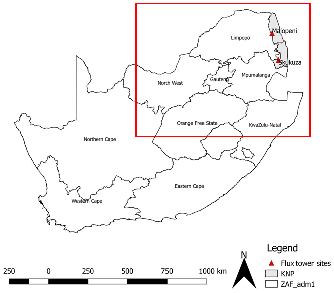
Figure 1 Maps indicating South Africa, Kruger National Park (KNP), flux tower sites (Skukuza and Malopeni) and the area considered for grid inter-comparison (red box).

2.2 Datasets

2.2.1 Soils texture data

The “SoilGrids” dataset from the international soil reference information centre (ISRIC) was used in this study to map soil types. The data are described in detail in the study by Hengl et al. (2017). The dataset has a spatial resolution of 250 m and is resampled to 25 km, firstly by resampling to 1 km and then to 25 km, using the nearest neighbour method to match the resolution of the soil moisture products. We acknowledge that resampling from fine to coarse resolution might introduce a bias towards certain soil types. However, the nearest neighbour method is suitable for resampling categorical data. Soils were classified into 12 dominant types ranging between sand and silty clay. The soil type data are available at various depths; here we only consider the data representing the surface (i.e. 0–5 cm).

2.2.2 Satellite observations

The European Space Agency climate change initiative (ESA-CCI) satellite-derived soil moisture datasets are used in this study (Dorigo et al., 2017; Gruber et al., 2019). These global datasets are based on passive and active satellite microwave sensors and provide surface soil moisture estimates at a resolution of ∼25 km (i.e. 0.25^∘) (Fang et al., 2016; Yuan and Quiring, 2017). The ESA-CCI merges soil moisture estimates from the active and passive satellite microwave sensors into one dataset (http://www.esa-soilmoisture-cci.org/, last access: 13 January 2020), using the backward-propagating cumulative distribution function method (Dorigo et al., 2015; Fang et al., 2016). A detailed description of the merged active and passive sensors and their functioning is provided by Fang et al. (2016), Dorigo et al. (2015) and Liu et al. (2012). The merging of active and passive sensors is based on their sensitivity to vegetation density, as the accuracy of these products varies as a function of vegetation cover (Liu et al., 2012). In this study, version 3.2 (v3.2) of the ESA-CCI soil moisture data is used. The merged data product is used in this study as it has better data coverage compared to the individual products. Missing data in satellite products are not unusual since retrievals are normally at an interval of 2–3 d (Albergel et al., 2012). However, data from each of the different sensor types are also considered for the evaluation of long-term seasonal cycles.

2.3 Models for simulating soil moisture

2.3.1 CCAM-CABLE

The variable-resolution atmospheric model CCAM developed by the CSIRO in Australia (McGregor, 2005; McGregor and Dix, 2001, 2008) was used to dynamically downscale ERA reanalysis data to 8 km resolution over north-eastern South Africa (Fig. 1) for the period 1979–2014. Similar downscaling of reanalysis data obtained over southern Africa using CCAM are described by Engelbrecht et al. (2011), Dedekind et al. (2016) and Horowitz et al. (2017). The ability of the CCAM model to realistically simulate present-day southern African climate has been extensively demonstrated (e.g. Engelbrecht et al., 2009, 2011, 2015; Malherbe et al., 2013; Winsemius et al., 2014). The CABLE soil sub-model expresses soil as a heterogeneous system consisting of three constituent phases, namely water, air and solid (Kowalczyk et al., 2006; Wang et al., 2011). Air and water compete for the same pore space, and the change in their volume fractions is due to drainage, precipitation, ET and snowmelt. In this model, there is no heat exchange between the moisture and the soil due to the vertical movement of water, as soil moisture is assumed to be at ground temperature. The soil is partitioned into six layers, with the layer thickness of 0.022, 0.058, 0.154, 1.085 and 2.875 m from the top layer. Only the top layer contributes to evaporation, while plant roots extract water from all layers depending on the soil water availability and the fraction of plant roots in each layer (Wang et al., 2011). Soil moisture is solved numerically using Richard's equation (Kowalczyk et al., 2006).

2.3.2 GLEAM

The Global Land Evaporation Amsterdam Model (GLEAM) version 3.1 is a set of algorithms used to estimate surface soil moisture, root-zone soil moisture and terrestrial evaporation using satellite forcing data (Martens et al., 2017). The method is based on the use of the Priestley and Taylor (1972) evaporation model, stress module, and rainfall interception model (Miralles et al., 2011). Three datasets from the GLEAM, namely v3a, v3b and v3c, were used in this study. Version 3a is based on satellite-observed soil moisture, snow water equivalent and vegetation optical depth, reanalysis radiation and air temperature, and a multi-source precipitation product. Versions 3b and 3c are satellite-based with common forcing data excluding soil moisture and vegetation optical depth; these are based on different passive and active microwave sensors, i.e. ESA-CCI for v3b and Soil Moisture and Ocean Salinity (SMOS) for v3c (Martens et al., 2017).

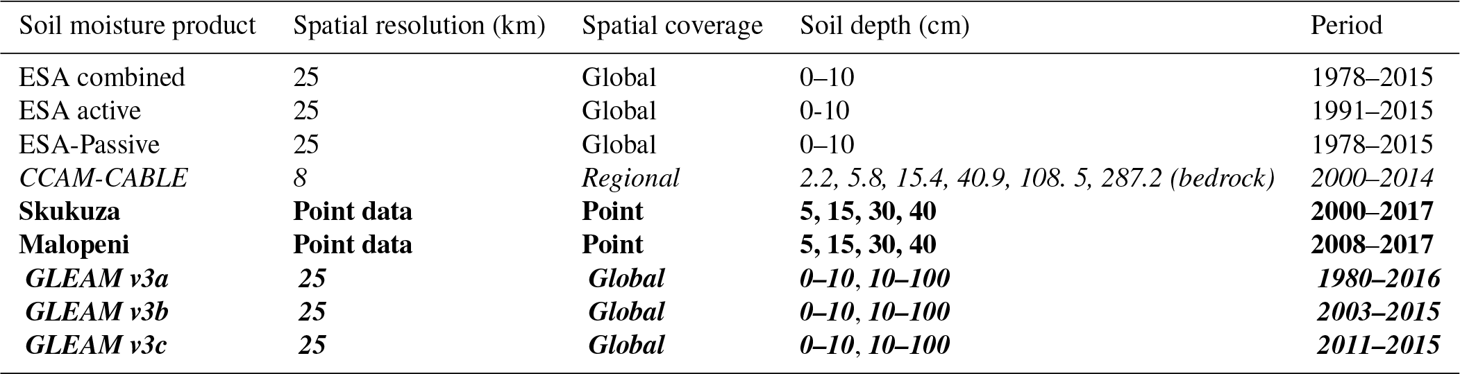
The different components of terrestrial processes (i.e. transpiration, open-water evaporation, bare soil evaporation, sublimation and water loss) are separately driven in GLEAM (Martens et al., 2017). Each grid cell in GLEAM contains fractions of four different land cover types, namely open water (e.g. dam, lake), short vegetation (i.e. grass), tall vegetation (i.e. trees) and bare soil. These fractions are based on the global vegetation continuous field product (MOD44B) except for the fraction of open water. The MOD44B product is based on the Moderate Resolution Image Spectroradiometer (MODIS) observations (Martens et al., 2017). Soil moisture is estimated separately for each of these fractions and then aggregated to the scale of the pixel based on the fractional cover of each land cover type. Root-zone soil moisture is calculated using a multi-layered water balance equation which uses snowmelt and net precipitation as inputs, and drainage and evaporation as outputs (Miralles et al., 2011). The depth of soil moisture is a function of land-cover type comprising one layer of bare soil (0–10 cm), two layers for short vegetation (0–10, 10–100 cm) and three layers for tall vegetation (0–10, 10–100 and 100–250 cm) (Martens et al., 2017). An overview of the soil moisture datasets used in this study is presented in Table 1.

2.4 Analysis approach and data processing

2.4.1 Statistical analysis

The first part of the analysis focuses on evaluating the monthly time series data of soil moisture products at the site level using observations. At a monthly timescale, the soil moisture seasonal cycle is assumed to well developed. A data threshold of 80 %, i.e. daily values are available for at least 80 % of the total number of days in a particular month, was used to average daily data to monthly. Months that did not meet the 80 % threshold were excluded from the analysis. Time series data for the evaluation sites were extracted from the soil moisture products, using the flux towers' geographical coordinates. The satellite products present averaged soil moisture data per grid cell. A distance-weighted average technique was used to interpolate the CCAM-CABLE model simulations to estimate soil moisture values representative of observational sites. The distance-weighted average method proved to be more representative than the nearest neighbour method, as the distance-weighted average method interpolates to the exact location of the tower by considering simulated values at grid points surrounding the location.

The soil moisture products were first converted to the percentage of volumetric soil moisture amounts for comparison purposes. As in Yuan and Quiring (2017), we assume that the soil moisture measurements at 5 cm depth are representative of the depth range 0–10 cm. In situ data at depths 15, 30 and 40 cm were combined using the depth-weighted average method to represent the 10–100 cm depth using Eq. (1):

$$\begin{array}{}\text{(1)}& {\mathrm{SM}}_{\mathrm{10}-\mathrm{100}}=\sum _{i=\mathrm{1}}^n{\displaystyle \frac{\mathrm{LT}}{\mathrm{SD}}}\times \mathrm{SM}\left(i\right),\end{array}$$

where SM₁₀₋₁₀₀ is the weighted soil moisture, n is the number of layers, LT is the layer thickness calculated as the difference between the soil depths, SD is the total soil depth of the soil profile and SM(i) is the daily in situ soil moisture values at the ith layer. The depth-weighted average method as presented in this study (Eq. 1) has been used in other studies such as that by Yuan and Quiring (2017). Similarly, the data at depths 2.2 and 5.8 cm and at 15.4 and 40.9 cm from CCAM-CABLE are averaged to represent 0–10 and 10–100 cm, respectively, using Eq. (1).

Table 1 Overview of soil moisture datasets: satellite (normal font) in percentage, modelled (bold and italic), simulation (italic) and in situ observations (bold) presented as a ratio (m³ m⁻³) of soil to moisture per unit area.

The soil moisture products used in this study (Table. 1) are under the same latitude and longitude projection. All the soil moisture projections are at the same spatial resolution of 25 km, except for the CCAM-CABLE model with a resolution of 8 km. The bilinear interpolation method was used to resample the CCAM-CABLE simulations from 8 to 25 km to match the resolution of the other soil moisture products. To evaluate how close the modelled soil moisture estimates are to in situ measurements we use the Taylor plots (Taylor, 2001) as well as the cross-wavelet analysis.

2.4.2 Cross-wavelet analysis

The cross-wavelet method analyses the frequency structure of a bivariate time series using the Morlet wavelet (Veleda et al., 2012). The wavelet method is suitable for analysing periodic phenomena of time series data, especially in situations where there is potential for frequency changes over time (Rosch and Schmidbauer, 2018; Torrence and Compo, 1998). The cross-wavelet analysis provides suitable tools to compare the frequency components of two time series, thereby concluding their synchronicity at a given period and time. In this study, the cross-wavelet analysis is used to qualitatively compare the cyclic patterns of the observations and the models' estimates. In particular, it is used to assess whether phase differences exist between dominating periodic features of the in situ observations and the models' estimates. The cross-wavelet analysis algorithm used is described in Rosch and Schmidbauer (2018) and is implemented within the “WaveletComp” package in the R software. This method has been used in other studies, such as that by Raj Koirala and Gentry (2012), for investigating the climate change impacts on hydrologic response.

The cross-wavelet analysis only applies to complete datasets (i.e. without missing values). Since the in situ observations have missing data, the multiple-imputation method as discussed in studies by Rubin (1987, 1996) has been used to gap-fill the in situ time series. The multiple imputation procedure is implemented in the “Amelia” package, also available in the standard repository for R packages. The number of imputed datasets was set to five and combined using Rubin's rules (Rubin, 1996). The multiple-imputation method is only applied to the Skukuza dataset for both the surface (Appendix Fig. A1a) and root zone (Fig. A1b). This is because the Skukuza data have fewer gaps compared to Malopeni data (Fig. B1). The imputed soil moisture observations are shown in Appendix A together with the statistics of the measures of the distribution for both the gap-filled and non-gap-filled datasets. The cross-wavelet analysis (Appendix C) is applied to non-stationary data using the default method (i.e. white noise) with the simulations repeated 10 times.

2.4.3 Seasonal soil moisture pattern

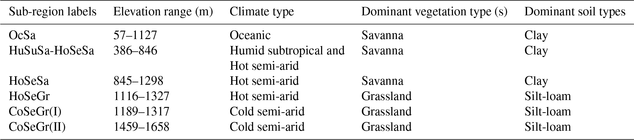
Six sub-regions are selected, based on a homogeneity assumption of climatic types (Fig. 2a), altitude (Fig. 2b) and soil types (Fig. 2c). The sub-regions are named based on their climate and vegetation types, namely oceanic savanna (OcSa), humid subtropical savanna and hot semi-arid savanna (HuSuSa-HoSeSa), hot semi-arid savanna (HoSeSa), hot semi-arid grassland (HoSeGr), and cold semi-arid grassland (CoSeGr). Each sub-region is characterized by an attribute (i.e. soil, vegetation and climate types) with the highest frequency. The dominant frequency is represented by at least 56 % of the 16 grid points for each attribute and for all sub-regions. This is with the exception of HuSuSa-HoSeSa, where the climate type humid subtropical and hot semi-arid have equal frequency. The selected subregions are summarized in Table 2 and plotted in Fig. 2. The vegetation types for the study area used here are presented in a study by Khosa et al. (2019). The sub-regions are selected to demonstrate how the models represent the patterns of daily soil moisture distribution at a regional scale. For each model and sub-region, seasonal distributions of modelled daily soil moisture values spanning the austral summer (December–February), winter (June–August), autumn (March–May) and spring (September–November) for the period 2011–2014 are summarized through a box-and-whisker plot. In summary, each sub-region data distribution consists of 16 grid points with each grid point having daily soil moisture values for each month of the respective seasons. Topographic features of the landscapes (i.e. slopes) of different aspect: north (N), east (E), south (S) and west (W) are also used to filter the respective seasonal distributions, thus revealing the soil moisture distributions' variation with thermal exposure or slope direction.

Table 2 A detailed description of the selected sub-regions indicating elevation (https://www.ngdc.noaa.gov/mgg/fliers/06mgg01.html, last access: 14 December 2019), climate (http://koeppen-geiger.vu-wien.ac.at/present.htm, last access: 14 December 2019), and vegetation and soil types (https://soilgrids.org, last access: 14 December 2019).

The second part of the analysis inter-compares model simulations and satellite estimates of soil moisture at a regional scale. The MI is calculated between the residuals of the de-trended and de-seasonalized time series at a regional scale between the CCAM-CABLE simulations and GLEAM estimates. The data are first de-trended and de-seasonalized before the MI is calculated to ensure that the computed MI is not attributed to the similarities in the trend and cyclic components of the signal.

The trend and cyclic components could be correlated and it is necessary to ensure that the MI is based on the residual components, which are the uncorrelated features of the soil moisture signal. In this way, the MI calculation presents a comparison matrix for inter-model soil moisture spatial pattern comparison. In particular, the MI gives a sense of similarity between the models, indicating the level of coincidence or overlap in the distribution of the residuals between a pair of CCAM-CABLE simulations and each of the GLEAM model estimates per grid point. In the case that MI values between models are low, the inter-model data reflect uncertainty in how the models capture the modelled processes.

The de-trending and de-seasonalizing of the time series removes the systematic components of the signal including bias. This is achieved through an approach reported in a study by Cleveland et al. (1990) where the “stl” package, available in the standard package repository in R, is used to de-trend the time series into its components. The MI calculation is described in Kraskov et al. (2004) and is applied in this study using the “varrank” package which is also available in the R CRAN repository. The MI measure calculated from the residual components of the respective soil moisture signals presents a robust way of assessing whether the respective models have a correspondence in spatial patterns of soil moisture across landscapes. In this paper, the MI is used as an index for classification of the models according to the coincidence in the distribution of residuals at the regional level. The MI is calculated for the daily time series ranging between 2011 and 2014.

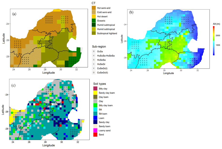
Figure 2 (a) Köppen–Geiger climate types (CT) across the study region at a 50 km resolution (http://koeppen-geiger.vu-wien.ac.at/present.htm, last access: 14 December 2019). Sub-regions are selected based on homogeneous climate types and named based on the vegetation and climate types, such as oceanic savanna (OceaSa), humid subtropical and hot semi-arid savanna (HuSuSa-HoSeSa); hot semi-arid savanna (HoSeSa), hot semi-arid grassland (HoSeGr) and cold semi-arid grassland (CoSeGr); (b) altitude (Alt, m) at the study region at a 25 km resolution (https://www.ngdc.noaa.gov/mgg/fliers/06mgg01.html, last access: 14 December 2019); and (c) dominant soil types (https://soilgrids.org, last access: 14 December 2019) per grid cell, at a resolution of 25 km.

3 Results and discussion

3.1 Evaluation of the satellite- and model-simulated seasonal cycle soil moisture

In this section, we discuss how the respective outputs reflect the key features of the observed soil moisture. As highlighted in the introduction, the variability of the simulation output, satellite-derived data and satellite-based model estimates are studied relative to the observations. Much focus is placed on investigating how well the periodic features of the soil moisture are reflected by the respective soil moisture datasets. The patterns of soil moisture at the study sites are mainly driven by rainfall, which is predominantly higher during the summer season and low in winter, as shown in Fig. 3. The long-term surface soil moisture for both the sites follows a pattern comparable to that of rainfall, as can be seen in Fig. 3.

3.1.1 Long-term seasonal cycles

The soil moisture patterns presented in Fig. 3 show that the study sites mainly contain higher soil moisture at the surface than at the root zone; this is shown by both the modelled soil moisture and the observations. This is indicative of water at these study sites being lost mostly through runoff and ET, and only a small fraction infiltrates the soil and is stored at the root zone. There is an acceptable similarity in the seasonal cycle of soil moisture (Fig. 3) between the various product outputs and the observations in terms of phase, especially at the surface. Notably, the observed soil moisture seasonal cycle at the surface at both Skukuza and Malopeni surface displays a local maximum in April and shows an increase from September to January. The cyclic qualitative features of the observed signal are captured by all the models. The soil moisture amplitudes are less pronounced in the root zone, but with November and October maxima at Skukuza and Malopeni respectively. In some instances, there is a lag such as the one presented by GLEAM v3c (i.e. maxima in October instead of November) at the surface, at both Skukuza and Malopeni. The soil moisture patterns are consistent with the observed rainfall cycle, which undergoes an onset in October and a cessation in April. The root-level soil-moisture pattern displays a signature of soil moisture retention, which relates to the persistence of dry and wet periods at various soil depths (Seneviratne et al., 2006). In light of this, it would be interesting to see how both the CCAM-CABLE simulation and the GLEAM soil moisture products depict the onset and cessation of the wet season; this will be discussed in Sect. 3.2. The CCAM-CABLE model outputs reflect that soil moisture reaches its highest values in March rather than April for Skukuza at the surface. The output does not reproduce the recorded elevated soil moisture for Malopeni in April at the surface. This is probably since the CABLE soil-moisture scheme does not take soil resistance into account (Whitley et al., 2016). Despite this, the long-term CCAM-CABLE monthly means of soil moisture are relatively comparable to the observation even in terms of magnitude (Fig. 3).

GLEAM v3c agrees with in situ measurements on the existence of an April soil moisture maximum, but it reflects the observed soil moisture increase, in November, a month earlier (i.e. in October). The satellite observations and GLEAM models (Fig. 3) display the same soil moisture signal as observed at the respective sites, indicating that the April maximum, in particular, is not an artefact of the point observations. We can safely deduce that the bias in GLEAM v3c is not induced by satellite-based forcing data; however, this calls for further investigations into the sensitivity of the model to its driving data at a high resolution. We anticipate that at high temporal resolution there is a strong variability in the in situ soil moisture signal which may not entirely be captured by both CCAM-CABLE and GLEAM, possibly due to their relatively low spatial resolution. The relatively low resolution (8 km in the horizontal) in the case of CCAM-CABLE, in particular, potentially has strong implications for how representative the effective drivers of soil moisture such as soil texture and vegetation covers are in terms of observations at specific sites.

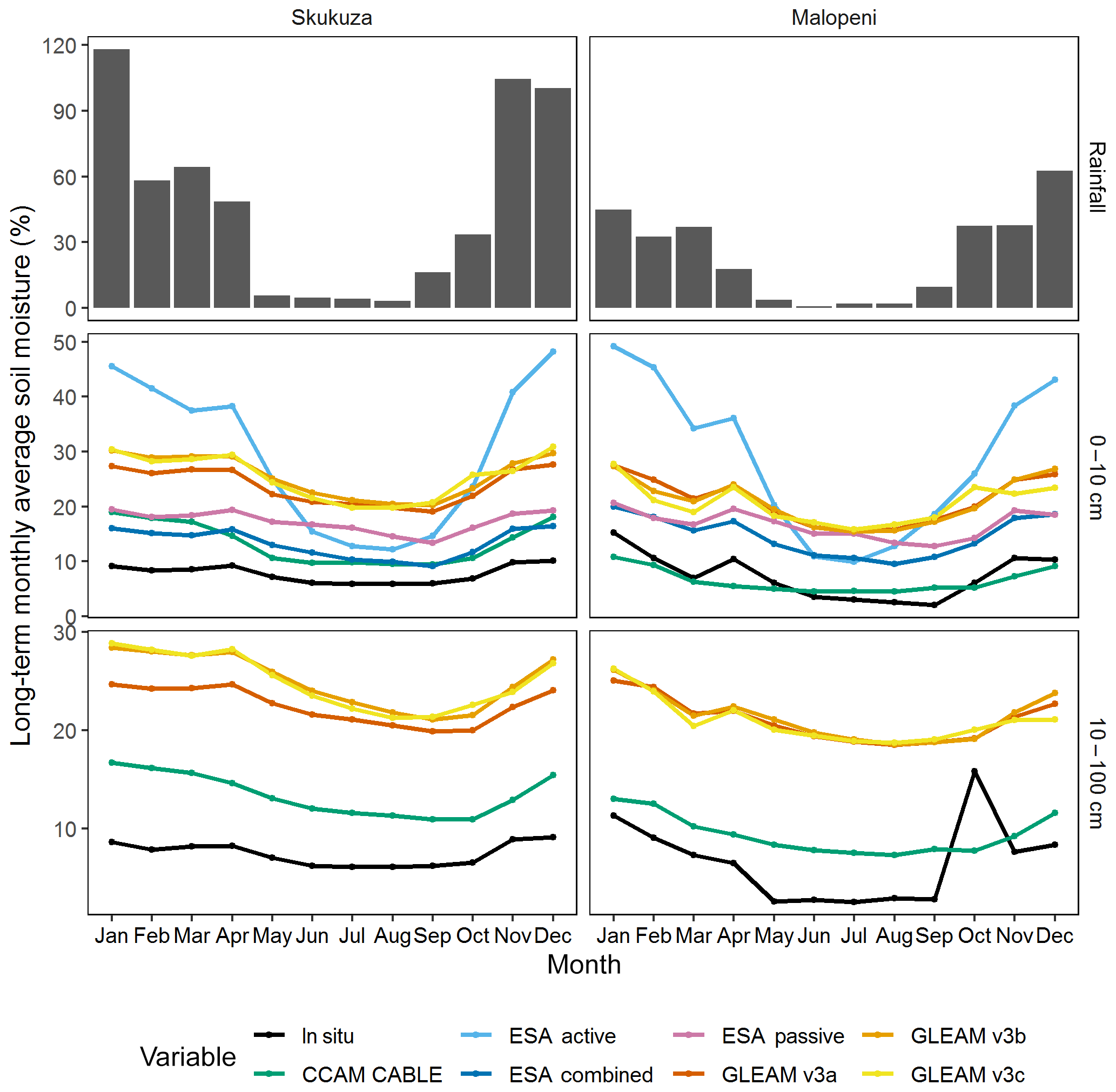
Figure 3 Seasonal variation in the long-term mean monthly rainfall (mm), surface (i.e. 0–10 cm) and root-zone (i.e. 10–100 cm) soil moisture, based on in situ observations and a variety of soil moisture products. The in situ data are collected from two sites, namely Skukuza (2001–2014) and Malopeni (2008–2013).

The GLEAM models (Fig. 3) are generally consistent with in situ measurements in estimating soil moisture in terms of phase, at both the surface and root zone. The magnitude of GLEAM v3a root-zone estimates is lower than those of the other GLEAM models at the Skukuza site. This can be attributed to the unique multi-source weighted ensemble precipitation (MSWEP) data used to force GLEAM v3a (Martens et al., 2017), which are different to the precipitation forcing data used in GLEAM v3b and v3c. We further observe that the GLEAM models, ESA and in situ observations have the same length of the dry period (i.e. about 4 months), except for the ESA active observation which has a shorter dry period (i.e. about 3 months).

The ESA active satellite product is known to work best for moderate to densely vegetated areas as opposed to savanna sites such as Skukuza and Malopeni, where tree cover is sparse (Dorigo et al., 2015). There is a minimal difference between the ESA-Passive and ESA combined satellite products in terms of both phase and magnitude. Generally, the ESA combined and ESA-Passive datasets have the least difference during the dry period for all sites. A number of studies evaluated the ESA products at a regional and global scale using in situ data and concluded that passive sensors displayed improved performance over bare to sparsely vegetated regions, whereas the active sensors perform better in moderately vegetated regions (Al-Yaari et al., 2014; Dorigo et al., 2015; Liu et al., 2012; McNally et al., 2016).

Using long-term monthly averages, both the CCAM-CABLE and GLEAM models can capture the intrinsic seasonality of the soil moisture signal for the sites as reflected by both the in situ and satellite observations. This is despite their being different in both the forcing data and model structure. Studies by Wang and Franz (2017) and Seneviratne et al. (2010) suggest that local factors (e.g. vegetation, soil and topography) mostly control soil moisture variability at spatial scales less than 20 km, rather than meteorological forcing. For a 14-year averaging period, undoubtedly the monthly means are sensitive to anomalously high precipitation, and hence soil moisture in some months. It is therefore instructive to investigate how well the simulated and estimated patterns of soil moisture compare with the in situ data monthly for the respective years.

3.1.2 Intra- and inter-annual variability in soil moisture

This section presents a quantitative evaluation of the soil moisture time series from the soil moisture products at a monthly time resolution. The level of agreement of the short-term seasonal cycles between the various outputs and observations is quantified in Fig. 4 using the Taylor plot. The Taylor plot presents three evaluation metrics, namely (1) the standard evaluation, which evaluates the amplitudes of the modelled soil moisture relative to the observations; (2) the centred root mean squared error (RMSE) measuring the distance in magnitude between the various products and the observations; and (3) the correlation coefficient measuring the agreement in phase.

Based on the correlation coefficient in Fig. 4a, we learn that there is an acceptable correlation between the observed and modelled soil moisture products at the surface ranging between 0.7 and 0.9. At the root zone, the correlation coefficients for the site range between 0.6 and 0.8. This indicates that there is more agreement in the soil moisture patterns at the surface than at the root zone. The disparity in the amplitude of variation at Skukuza and Malopeni, as reflected by the standard deviation and the normalized bias in Fig. 4a and b respectively, shows that it remains difficult for the models to predict the magnitude of in situ soil moisture and its evolution over time, especially for the root zone, where all the models bear very little coherence with observations. The coefficient of determination (Fig. C1) also shows that the models are able to explain at least 50 % of the observed soil moisture variability at the root zone and the surface for both sites. At the root zone, the models can only explain between 38 % and 53 % of the variability in the observed soil moisture at Skukuza and Malopeni respectively. On account of missing values, the R² values presented in Fig. C1 are based on different sample sizes. Therefore, their interpretation is made with this issue in mind. In particular, it is inconclusive whether the simulations and estimates are more comparable at Malopeni relative to Skukuza.

For the Skukuza site, we learn in Fig. 4a that the standard deviation for the surface and root-zone soil moisture observation is around 4.5 % and 4.7 % respectively. The standard deviation values for the surface and root-zone time series, for the various modelled soil moisture products, are mostly within the ranges 4 %–5 % and 2.7 %–5 % at the respective depths. In general, the standard deviation for modelled data is not at the perfect overlap with that from observation. The GLEAM products mainly present relatively closer standard deviations with the observations, while the CCAM-CABLE and ESA combined products show standard deviation values slightly lower than those of the observations, indicating a slight underestimation by these products. At the root zone the soil moisture standard deviation is relatively lower (i.e. about 1.5 %) for the observations while all other soil moisture projects reflect much higher standard deviation, indicating an overestimation of the root zones soil moisture by these products. At Malopeni, we learn that the standard deviation for observed soil moisture values is about 4.7 % at the surface and 3.2 % at the root zone. In both cases the models present a standard deviation with a range closer to that of the observed root-zone values. For this particular site, the agreement between the various products and the observations is more pronounced at the root zone (RMSE ranges between 1.8 % and 2.3 %) than at the surface (RMSE ranges between 2.1 % and 3.5 %).

On the basis of a comparisons of standard deviations, we can conclude that the pattern variations for different soil moisture products are not of the right amplitude at both the surface and root zone for the two respective sites. The amplitude of the pattern of variation among most of the models at the root zone, particularly at Skukuza, is relatively incoherent with that of the observations. At the root zone, this is consistent with that of the models at Malopeni but not Skukuza. We learn from Fig. 4b that the models are mostly biased towards an overestimation (i.e. values above the horizontal line) of the observed soil moisture. The overestimation is more pronounced at the root zone relative to the surface. This is mostly true at both Skukuza and Malopeni. We also learn that the models mainly present a pronounced overestimation bias at Malopeni compared to Skukuza. The GLEAM and ESA combined products predominantly show higher bias towards overestimation compared to the CCAM-CABLE model. The CCAM-CABLE model shows the least bias relative to the other soil moisture products at both the surface and the root zone. At the Skukuza site, the CCAM-CABLE and ESA combined products show an underestimation of the observed soil moisture at the surface.

The ESA combined satellite product presents a similar performance to the GLEAM products at both Skukuza and Malopeni. The ESA data have been shown to generally capture soil moisture in different regions and climatic zones of the world (Loew et al., 2013; McNally et al., 2016; Wang et al., 2016; Zeng et al., 2015). Our study confirmed (Fig. 4) that the ESA combined product captures local (i.e. South African semi-arid) conditions within an acceptable amount of certainty. A study conducted by Yuan and Quiring (2017) assessing the performance of CMIP5 models at both the surface and root zone concluded that the models performed better at the root zone relative to the surface. These results contradict the findings of this study, where we generally observe better agreement between soil moisture products and in situ measurements at the surface than at the root zone. Based on the general picture of the extent to which the soil moisture products proved to be representative of the quantitative features of the soil moisture signal, as driven by precipitation at the site, it is compelling to further resolve qualitatively, for each periodic soil moisture feature, how the various outputs compare with the in situ observations. To that effect, the next section will present the results from a cross-wavelet analysis of the soil moisture output and the in situ observation.

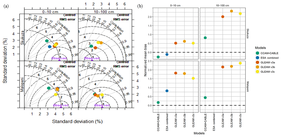
Figure 4 (a) Taylor plots quantitatively comparing monthly modelled soil moisture to observations at Skukuza (2001–2014) and Malopeni (2008–2013), at both the surface (0–10 cm) and root zone (10–100 cm). The vertical solid grey lines represent the correlation coefficient. The broken black line cutting through the semi-circle broken black lines represents the standard deviation of the in situ observation. The semi-circle broken black lines represent the centred root mean squared error. (b) Normalized mean bias (NMB) of surface (0–10 cm) and root-zone (10–100 cm) soil moisture, computed between the various soil moisture products and the in situ observations at Skukuza and Malopeni.

3.1.3 Cross-wavelet analysis

In this section, a cross-wavelet transform constructed from two continuous wavelet transforms applied to the modelled and observed time series respectively is studied. The cross-wavelet analysis is instrumental in depicting the relationship in time and frequency space between two time series. This is achieved by analysing localized intermittent oscillations in the respective time series. By looking at the regions in time and frequency space with relatively large common power (represented by red colours; Fig. 5) and a consistent phase relationship (depicted by arrows), we gain a sense of whether there is a physical relationship between the observed and modelled soil moisture fields. Looking at Fig. 5 we learn that the soil moisture signal components with a common power are immediately identifiable and are portrayed as having periods (y-axis values) that lie between 8 and 15 months. This is depicted by dark red regions bound by white lines, which mark the region with 10 % significance level (i.e. 90 % confidence level). On comparing the surface and root-zone cross-wavelets, we can conclude that the statistically significant cyclic components with the dominating common power are generally between the periods of 8 and 15 months. This can be associated with seasonal soil moisture variation as driven by meteorological drivers, most of which have a return period of about a year.

From Fig. 5a we can see based on the alignment of the arrow (Fig. C1) that the most common high-power signals between modelled and observed data are in phase, in some instances with a time lag. This is identified by the direction of the arrows which are inclined either upwards or downwards. See Fig. C1 in Appendix C for an interpretation of the direction of the arrows. From the graph of the phase difference, we can see that there is an interchange of years in which the modelled fields are leading or lagging in phase; however, the phase difference is mostly very small. There is a time lag of 2 d on average between CCAM-CABLE simulations and in situ observations at the period of about 12 months, and a lag of about 6 d on average between GLEAM v3a and the in situ observations at the surface. At the root zone, we observe a wider lag of between 14 and 24 d between the soil moisture products (i.e. CCAM-CABLE and GLEAM v3a) and the observations. This further confirms that there is a better agreement between the soil moisture products and the observation at the surface than at the root zone.

In all models, precipitation is a source of soil moisture at the surface while heat and wind are sinks of moisture from the surface. As mentioned earlier the models introduce different assumptions about dominating drivers of root-zone soil moisture for instance, which may potentially explain the existence of broader time lags at the root zone. We further observe, in Fig. 5, that there is an agreement between the models and observations on the seasonal and intra-annual signal of soil moisture at Skukuza; this is shown by orange depicted regions on the cross-wavelet graphs. These are the signal components mainly ranging between the periods of 2 to 6 months. This could be associated with anomalous years where the transition periods between the austral winter and summer may have months with below (dry) or above (wet) normal soil moisture conditions. Despite these periods having a relatively high common power, they are not demarcated as statistically significant.

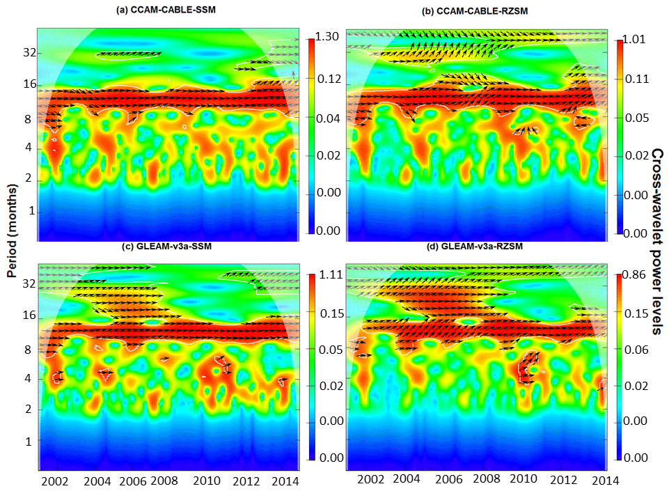
Figure 5 Cross-wavelet power spectrum of surface (SSM, 0–10 cm) and root-zone (RZSM, 10–100 cm) soil moisture between in situ observations, CCAM-CABLE (a, b) and GLEAM v3a (c, d) at Skukuza respectively. The white contour lines indicate periods of significance at 10 %. The arrows pointing to the right indicate that the models and in situ observation are in phase while arrows pointing left reflect that the models are anti-phase. The case where in situ observations are leading either CCAM-CABLE or GLEAM v3a is indicated by arrows pointing straight down. The dome shape (shaded areas) represents the cone of influence between 2001 and 2014. The red colour indicates weak variation while blue indicates the strong variation between the respective time series.

It would be interesting to establish how the qualitative insight gained in understanding the models' ability to capture the observed soil moisture signal at the two respective sites will translate to a regional level. An upscaling of the evaluation done at a point is not possible in the absence of site observations at a regional level. The rest of the discussion in this paper is dedicated to an inter-comparison of process-based model outputs and satellite-derived model outputs. The idea is to discuss the model outputs in connection with the broader landscape classes within the region.

3.2 Linking soil moisture patterns to landscapes

So far we have investigated the capabilities of the models in capturing the temporal features of soil moisture at the flux tower sites. An interesting question to address is, to what extent do the respective models compare in capturing soil moisture organization across different landscapes as characterized by altitude range, climatic zone, dominant soil, biome types and slope aspect within the considered 25 km resolution. In the case where there are no in situ soil moisture fields, we may not reliably tell which product is the most representative of the soil moisture organization; however, we can classify the models on the basis of their shared patterns at the selected landscapes.

Fig. 6 summarized the pattern of daily moisture distribution for the chosen six sub-regions for the austral summer (DJF), winter (JJA), autumn (MAM) and spring (SON) for the year 2011 to 2014. Each sub-region is represented by 16 grid points with each grid point having daily soil moisture values that span the respective season for the years 2011–2014. By looking at the interquartile ranges of the box-and-whiskers plot we can see that the characteristic seasonal feature of soil moisture signal is reflected by all models at all landscapes. In particular, all models are consistent in reflecting soil moisture distribution interquartile ranges, and hence the median, as highest in DJF and lowest in JJA.

By comparing the spread and the median of soil moisture distribution across models, we can conclude that for the region OcSa, which is characterized by predominance of clay soil and relatively low elevation range, there is no clear variation of soil moisture spread that could be associated with models or the respective south- and east-facing slopes in the humid (HuSuSa-HoSeSa) and hot semi-arid (HoSeSa, HoSeGr) regions; the soil moisture spread is comparable between CCAM-CABLE and ESA but relatively lower to that of the GLEAM models. It is worth reiterating at this point that GLEAM models also show higher soil moisture values relative to the in situ observations at the Malopeni and Skukuza flux tower sites, which share the same elevation range and climate type as region (HuSuSa-HoSeSa). For the three landscapes, there is no clear pattern which distinguishes the organization of soil moisture according to slope direction. In the case regions (OcSa, HoSeSa, HoSeGr, CoSeGr(I)) highly overlapping distributions indicate that soil type, topographic or thermal exposure indices used could not be instantly associated with dominant or identifiable soil moisture patterns among the respective models. For the cold and high-lying semi-arid regions, CoSeGr(I) and CoSeGr(II), CCAM-CABLE shows a noticeable variation in soil moisture with slope aspect, in which case north-facing slopes turn out to have lower soil moisture than south- and west-facing ones. For the north-facing slopes of the two regions, the relatively lower soil moisture values for CCAM-CABLE are corroborated by that of the ESA combined model, which generally portray comparatively low soil moisture values for the two high-lying cold semi-arid regions. It is a well-known fact that along the Drakensberg range, which is close to the regions CoSeGr(I) and CoSeGr(II), north- and east-facing slopes have more sunshine exposure than the south- and west-facing slopes (Bristow, 2019). Notably, the CCAM-CABLE, ESA combined and GLEAM models reflect contrasting patterns with slope aspect for the high-lying areas. Whereas all models produce overlapping soil moisture distribution or relatively flat terrains (i.e. OcSa, HuSuSa-HoSeSa, HoSeSa and HoSeGr) with consistent seasonal variations, we note that the soil moisture distribution reflects a delineation with slope direction on high-lying areas. This points to a possibility of the existence of dominant drivers such as thermal exposure. This calls for model evaluation against observations in these regions and driver-specific sensitivity tests. Such an evaluation could potentially yield valuable information on which model assumptions or schemes could benefit from further refinements, taking into account dominant drivers and slope-dependent soil moisture processes for the landscape.

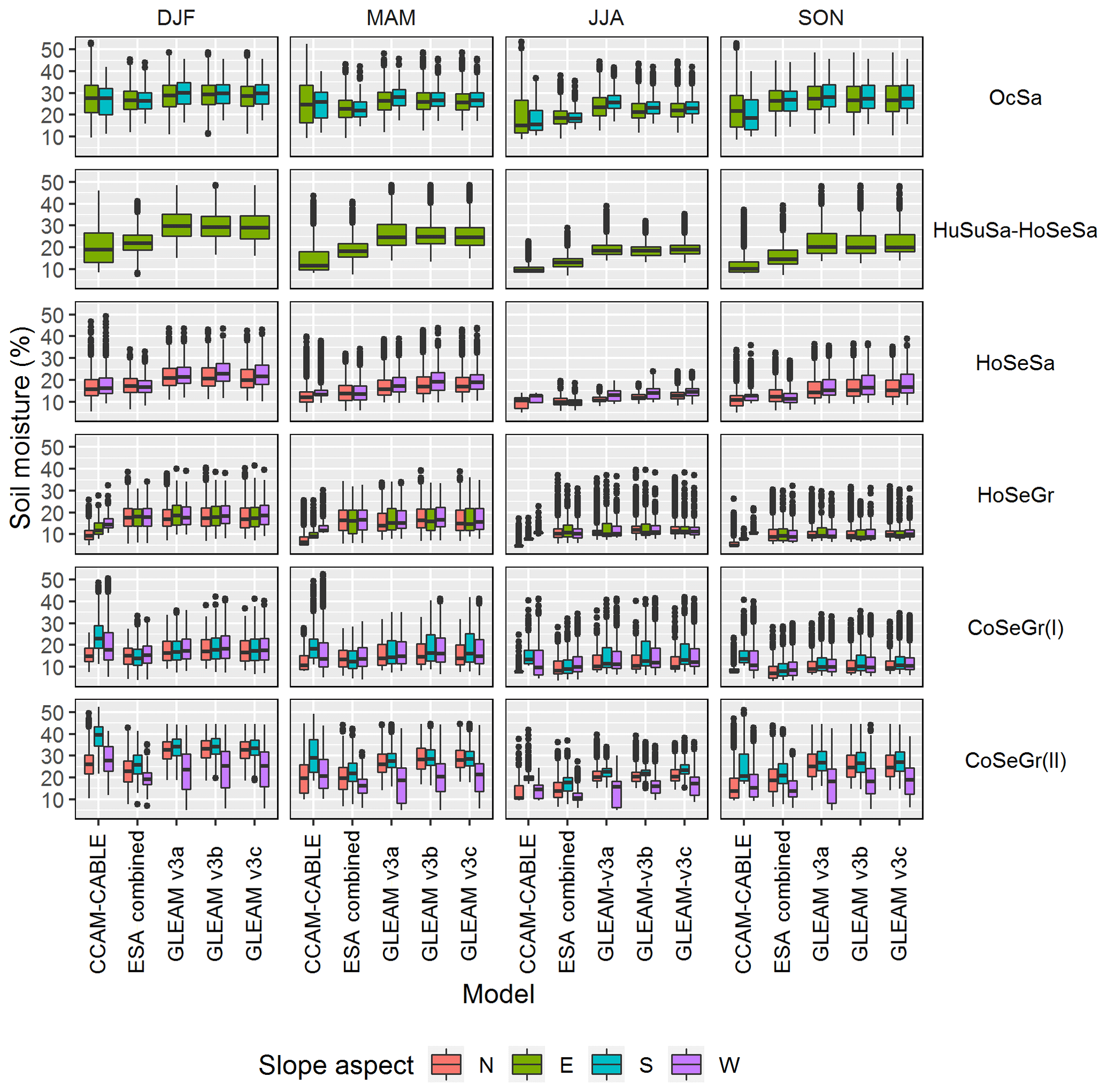
Figure 6 Comparison of modelled soil moisture patterns across sub-regions, namely oceanic savanna (Ocsa), humid subtropical and hot semi-arid savanna (HuSuSa-HoSeSa), hot semi-arid savanna (HoSeSa), hot semi-arid grassland (HoSeGr), and cold semi-arid grassland (CoSeGr). The sub-regions are also based on increasing altitude and slopes of different aspect, i.e. north (N; red), east (E; green), south (S; blue) and west (W; purple). The box plots show the distribution of the seasonal (i.e. summer, DJF; autumn, MAM; winter, JJA; and spring, SON) soil moisture data points per model within the respective regions. Each of the sub-regions consist of 16 grid cells for various slope aspects; therefore, each box plot contains 30 data points for each month of the 3-month season for the 4-year period (2011–2014) for each product and slope aspect, i.e. n= SP$\cdot \mathrm{3}\left(\mathrm{30}\right)\cdot \mathrm{4}$, where SP is the number of points for each slope aspect.

For the selected landscapes, we have learnt that the three GLEAM models mostly reflect a spread of soil moisture values which is largely overlapping, while CCAM-CABLE shows the existence of distinct moisture distributions that could be associated with slope aspect, especially in high-lying regions. A clear continuous picture of how CCAM-CABLE compares with GLEAM models across the entire study domain can be obtained by investigating how different joint distributions of a pair of CCAM-CABLE and GLEAM residuals per grid point compare to a product of their marginal distributions. This is best quantified by the MI, which is an information theory function that can be used as a measure of similarity between a pair of time series of residuals. The compared time series are computed on a common grid point for the respective models. The MI is equal to zero when the joint distribution of the pair coincides with the product of the marginal for the respective models. This suggests that the respective models are portraying independent signals. For the studied datasets we expect that the MI values should be greater or equal to 2 in the extreme case when the two pairs are identical. Figure 7 depicts the MI which is calculated from a pair of de-trended and de-seasonalized time series of monthly averaged soil moisture for CCAM-CABLE and each of the three versions of GLEAM. The de-trending and de-seasonalizing of each pair also lead to the removal of systematic biases. The obtained MI values are mostly equal to or greater than 0.5. This is true for both the surface and root zone. It is desirable to have the MI for all satellite-derived products; however, the ESA products did not have enough spatial data points to yield a fair comparison.

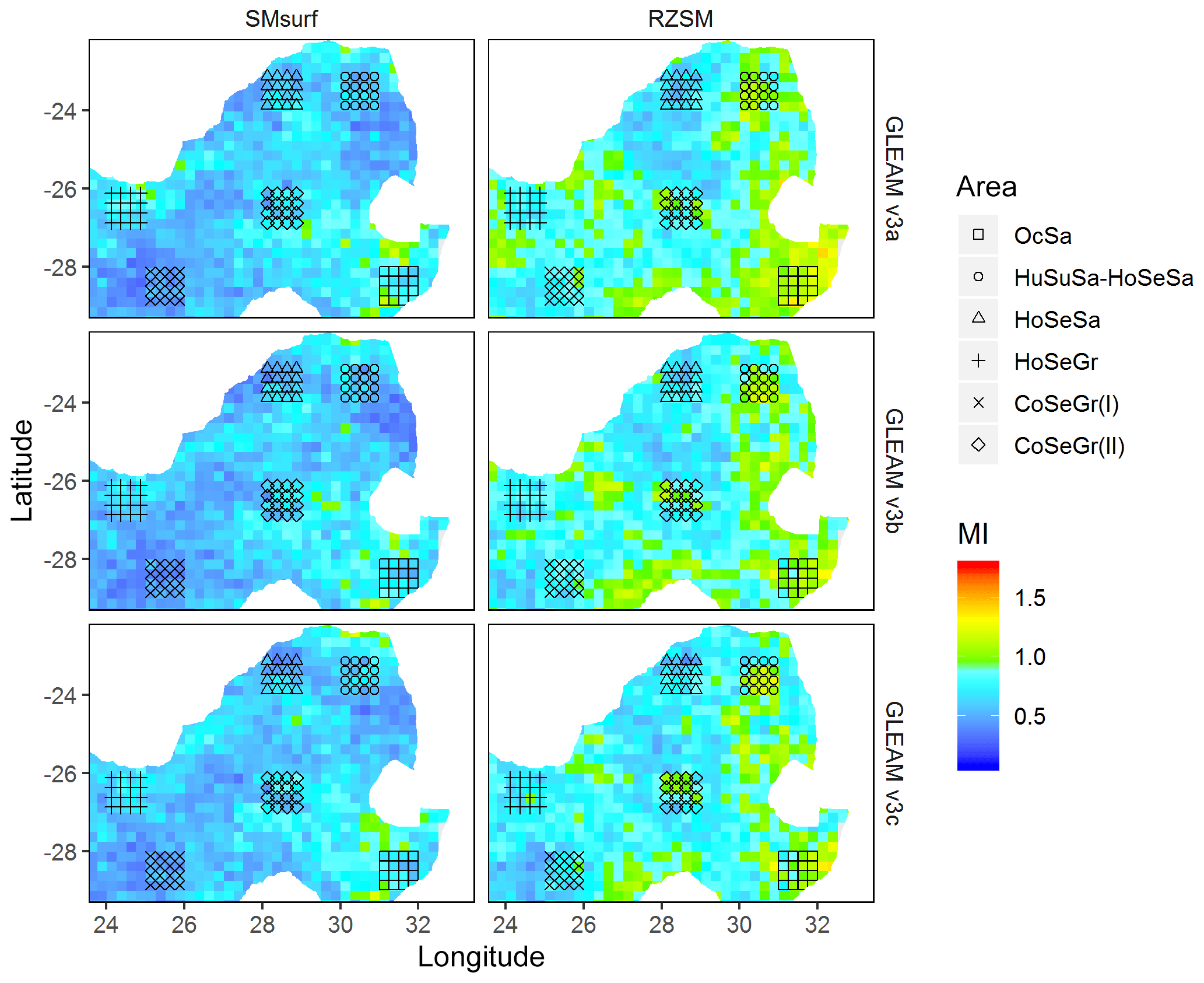
Figure 7 Mutual information (MI) computed on the residuals of monthly time series (2011–2014) of surface (SMsurf, 0–10 cm) and root-zone (RZSM, 10–100 cm) soil moisture, between CCAM-CABLE simulations and GLEAM models estimates. The studied sub-regions of interest are represented by different shapes on the maps, namely oceanic savanna (Ocsa), humid subtropical and hot semi-arid savanna (HuSuSa-HoSeSa), hot semi-arid savanna (HoSeSa), hot semi-arid grassland (HoSeGr), and cold semi-arid grassland (CoSeGr).

We can also see in Fig. 7 that the MI at the root zone is higher than at the surface; this could be suggestive of the sensitivity of soil moisture to the driving processes being comparable between both GLEAM and CCAM-CABLE models at the root zone. The MI pattern for both the surface and root zone complement the box-and-whisker plot, indicating that the coincidence in the soil moisture values is highest in the proximity of the lowest-lying OcSa, which is dominated by the clay soil. For this region, the MI values mainly range between 1 and 2. CCAM-CABLE has been depicted as having low soil moisture values relative to all versions of GLEAM on part of the humid savanna region (HuSuSa-HoSeSa) for the surface. We can also see that, on the humid savanna which includes region (HuSuSa-HoSeSa), that the models predominantly have low MI values ranging between 0 and 1 at the surface. The lowest MI values at the surface are also noticeable on the cold semi-arid high-lying grasslands in the neighbourhood of regions CoSeGr(I) and CoSeGr(II). From Fig. 7, we can conclude that the study region is dominated by grid points with relatively high MI values that fall within the range [0.5–2). Lower MI values for the high-lying regions are indicative of a pronounced model uncertainty when it comes to the models' response to processes that drive soil moisture for the region. While higher MI values, as seen in the rest of the regions, gives an indication that the respective models comparably responds to the dominating processes that drive soil moisture variation. This is the case at least qualitatively.

4 Conclusions

In this study, the ability of a process-based simulation model (CCAM-CABLE), satellite data-driven model estimates (GLEAM) and satellite observations (ESA active, passive and combined) are evaluated against site-specific in situ observations from two flux tower sites, namely Skukuza and Malopeni. The evaluation was done for two soil depths, namely the surface (i.e. 0–10 cm) and root-zone soil moisture (i.e. 10–100 cm), to understand how the respective data products capture the characteristic patterns of soil moisture. The evaluation included an assessment of qualitative features of long-term (i.e. multi-year) and short-term (i.e. monthly) averages of the soil moisture signal relative to the in situ measurements. All the models have a correlation that is greater than 0.6 at all soil depth and sites; however, not all models are able to capture the soil moisture magnitudes and their associated change over time at the root zone specifically, where the there is a pronounced incoherence as reflected by the bias score. All GLEAM soil moisture products presented a higher soil moisture magnitude range compared to observations while CCAM-CABLE and ESA combined outputs turn out to be relatively closer in magnitude to the observation at all depths at both Malopeni and Skukuza. The systematic difference in magnitude between the model output and observation may emanate from the difference in spatial scale between in situ measurements and the rest of the products. We also learn from this study that all GLEAM models compare well with the in situ observations in reflecting the seasonality of soil moisture. This is despite the noted systematic bias of the soil moisture magnitudes in the GLEAM products. The models mostly show a bias towards overestimation of the observed soil moisture at both the surface and root zone, with the CCAM-CABLE showing the least bias.

A wavelet analysis was used to reveal, at a qualitative level, how periodic features compare between the CCAM-CABLE model, GLEAM models and in situ observations. We learned that at the surface, high-power common features of the surface soil moisture signal are in phase with observations and come at a periodicity of about 12 months. We also learned that high-power common soil moisture signals at the root zone have a relatively pronounced time lag. The time lag is of a timescale not exceeding a month at all soil depths (i.e. it lies between 5 and 20 d) for the periods ranging between 2001 and 2014 between CCAM-CABLE and GLEAM v3a.

The study also investigated, through the use of mutual information (MI), how different joint distributions of pairs of grid points among CCAM-CABLE and the respective GLEAM models compare with a product of their marginal distributions. This gave a basis for classifying the models according to their similarity or dependence in capturing soil moisture responses to the underlying drivers. In this case, the emphasis is on evaluating the extent to which both approaches have a joint variation or shared MI. The analysis has successfully revealed that both the simulation and model estimates have a high similarity at the root zone as opposed to the surface for all GLEAM model outputs. The difference in the surface soil moisture between the CCAM-CABLE simulation and GLEAM model outputs in high-lying areas opens up interesting questions relating to the extent to which the influence of different drivers of soil moisture is represented by the two approaches. To understand this, future research will benefit from investigating the sensitivity of the models to changes in soil moisture drivers, particularly change in vegetation cover and soil type, on soil moisture memory. It would also be interesting to unearth the soil moisture organization for the respective models at much higher spatial resolution so that processes that drive soil moisture may be reliably attributed to the patterns of the soil moisture signal. Despite CCAM-CABLE and GLEAM having relatively high MI for the majority of landscapes, application of these model outputs should take into account that systematic biases do exist and that there is a high model uncertainty, particularly in high-lying areas.

Appendix A: Multiple imputation

Table A1 Statistics of the distribution of the imputed and observed time series of surface and root-zone soil moisture at the Skukuza site.

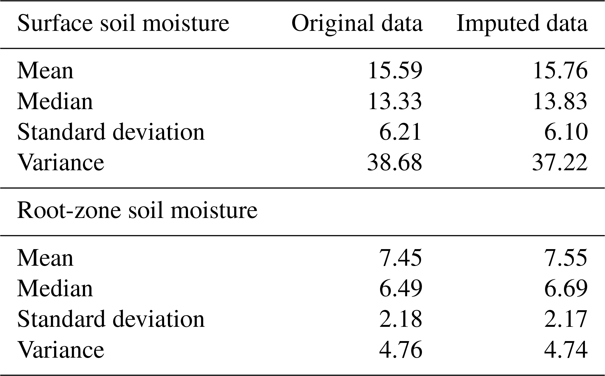
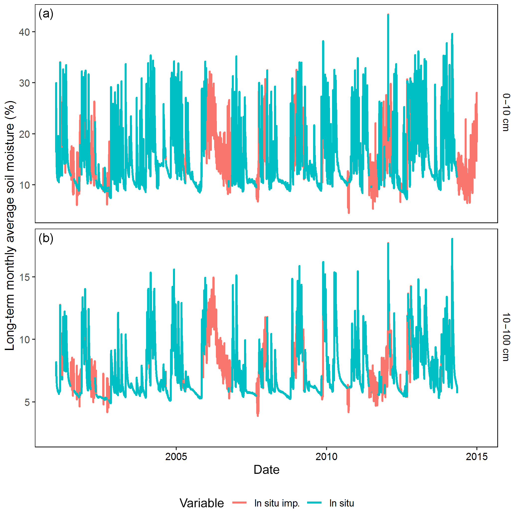
Figure A1 Daily (a) surface and (b) root-zone soil moisture time series at Skukuza showing the imputed parts (red) of the time series and the observed parts (blue).

Appendix B: Comparison of modelled and in situ soil moisture

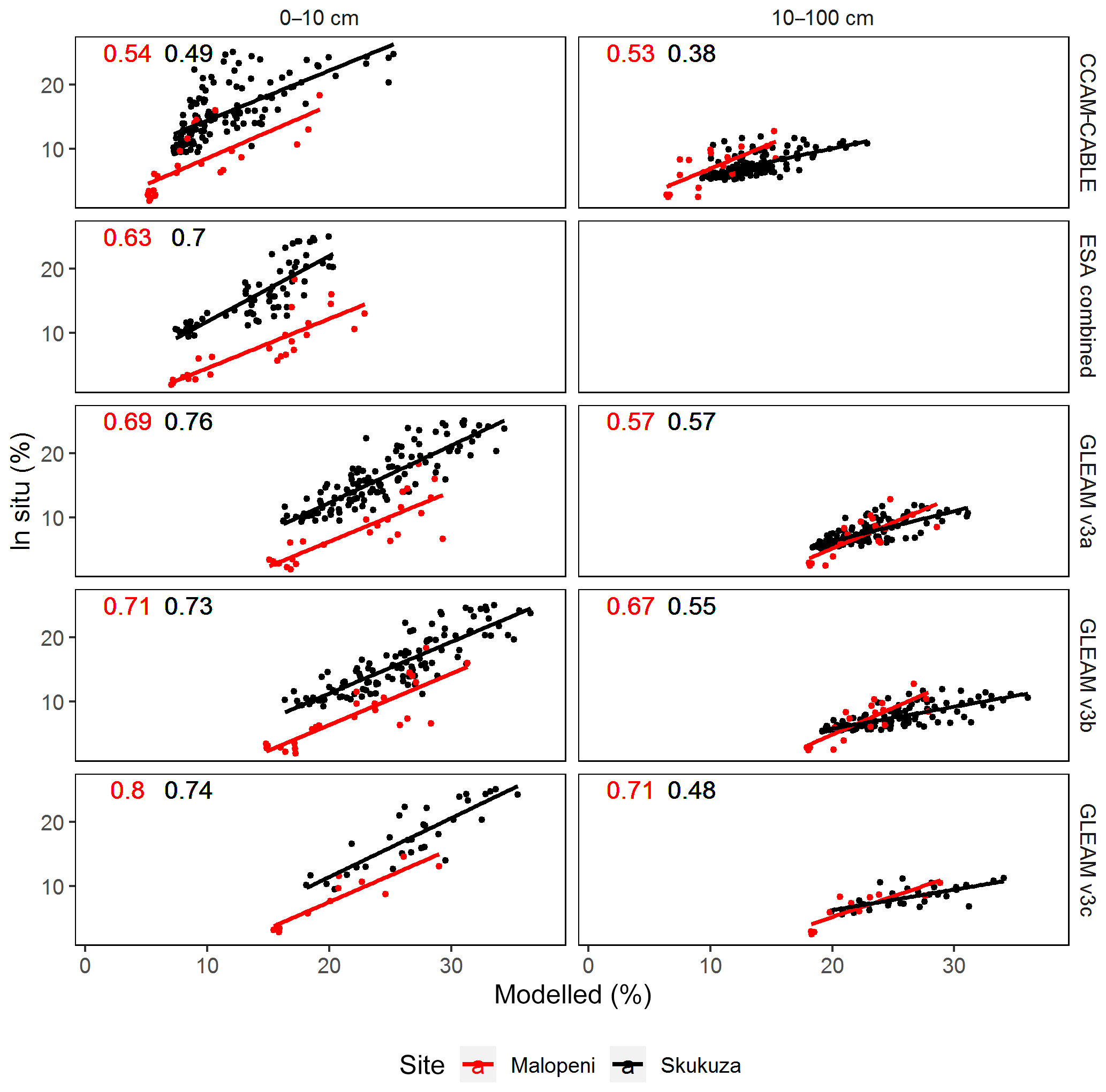
Figure B1 Quantitative monthly comparison between soil moisture products and observations at Skukuza (black; 2001–2014) and Malopeni (red; 2008–2013), at the surface (0–10 cm) and root zone (10–100 cm), using the coefficient of determination (R² ) depicted by the numbers in the top left of the plots.

Appendix C: Cross-wavelet analysis

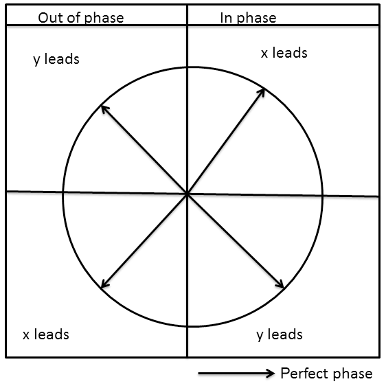
Figure C1 Phase interpretation between two time series x and y. When series x leads, y lags and vice versa. This figure is inspired by a study by Rosch and Schmidbauer (2018).

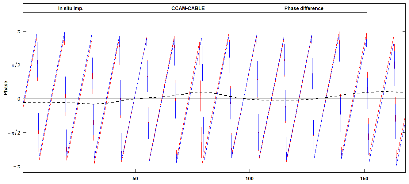
Figure C2 Phase difference between surface soil moisture simulated using CCAM-CABLE, and GLEAM v3a at Skukuza between 2001 and 2014 at period 12 at the surface.