Global partitioning of runoff generation mechanisms using remote sensing data

A set of complex processes contribute to generate river runoff, which in the hydrological sciences are typically divided into two major categories: surface runoff, sometimes called Hortonian flow, and baseflow-driven runoff or Dunne flow. In this study, we examine the covariance of global satellite-based surface water inundation (SWI) observations with two remotely sensed hydrological variables, precipitation, and terrestrial water storage, to better understand how apparent runoff generation responds to these two dominant forcing mechanisms in different regions of the world. Terrestrial water storage observations come from NASA’s Gravity Recovery and Climate Experiment (GRACE) mission, while precipitation comes from the Global Precipitation Climatology Project (GPCP) combined product, and surface inundation levels from the NASA Surface WAter Microwave Product Series (SWAMPS) product. We evaluate the statistical relationship between surface water inundation, total water storage anomalies (TWS; TWSAs), and precipitation values under different time lag and quality control adjustments between the data products. We find that the global estimation of surface inundation improves when considering a quality control threshold of 50 % reliability for the SWAMPS data and after applying time lags ranging from 1 to 5 months. Precipitation and total water storage equally control the majority of surface inundation developments across the globe. The model tends to underestimate and overestimate at locations with high interannual variability and with low inundation measurements, respectively.

1 Introduction

There is a long history of research concerning the mechanisms that control runoff generation at the terrestrial land surface (e.g., Beven and Kirkby, 1976; Pearce et al., 1986; Lyon et al., 2006; Vivoni et al., 2007; Kirchner, 2009). In brief, it is generally well accepted that two major mechanisms are responsible for surface water formation: (1) excess precipitation and the limitation of infiltration causing surface runoff or (2) the rising of the water table and deeper soil moisture to push more water into stream networks at a low topography. If precipitation rates exceed infiltration rates, then precipitation dominates surface inundation development and is typically defined as Hortonian flow. If precipitation successfully infiltrates and soils become saturated, then subsurface soil water storage will dominate surface water formation, typically described as Dunne flow. These are core concepts within terrestrial hydrology; however, there are limited observational studies on these runoff generation mechanisms at scales larger than a catchment. We are not aware of any studies that have assessed the contributions to surface water formation over a global domain. However, using existing data on global precipitation and water storage and considering how these two mechanisms influence surface inundation development, it is now possible to examine surface runoff mechanisms across a range of land surface conditions.

Satellite observations offer a means to observe changes in hydrology over a global domain, presenting a distinct advantage over in situ observations in representing a variety of hydrological mechanisms and processes across ecosystems and land cover types. Previously published work has utilized a variety of measurements of catchment or basin antecedent conditions, such as soil moisture or vertically integrated water storage, to assess the influence of soil water on runoff generation (e.g., Koster et al., 2010; Reager et al., 2014). NASA’s Gravity Recovery and Climate Experiment (GRACE) mission (Tapley et al., 2004) offers a 15+-year observational record on the state of terrestrial water storage globally. GRACE measures a change in the gravitational potential that is often linearly related to the amount of water stored at the land surface beneath the satellites. While these measurements are increasingly uncertain at resolutions beneath 150 000 km², they offer a robust and highly accurate means to measure changes in storage for areas larger than 150 000 km² (e.g., Wahr et al., 2006; Wiese et al., 2016) and offer a globally gridded dataset of total water storage anomalies (TWSAs) that is relatively easy to use. Previously, GRACE observations have been applied to develop a flood potential index and to characterize the intensity of certain flood events based on storage preconditioning or “flood potential” (Reager and Famiglietti, 2009; Reager et al., 2014). These studies serve as proof that integrated basin water storage is significant in understanding surface inundation changes.

There is also extensive literature relating to the influence of precipitation on surface inundation (Guo et al., 2012; Kirchner, 2009). The Global Precipitation Climatology Project (GPCP) offers a globally gridded precipitation dataset that optimally combines satellite, in situ, and land radar measurements into a single best product (Adler et al., 2003). This precipitation dataset can be used to assess the relationship between rainfall and surface water inundation (SWI) globally.

The satellite observations of TWSA and precipitation can be related to observations of surface water formation from the Surface WAter Microwave Product Series (SWAMPS) (Schroeder et al., 2014a) dataset to better understand runoff generation. SWAMPS was created based on optical and radiometric observations of surface reflectance that are often associated with water. These observations are expressed in terms of fractional inundation, i.e., the percentage of land occupied by surface water at a 0.25^∘ grid resolution globally. Schroeder et al. (2014a) provide a quality control map expressed as likelihood or confidence that allows a user to mask out unreliable data at the quality threshold of their choosing.

For this study, we imagine a global land surface model, typically run at 1^∘ globally (or at best, 0.25^∘ globally), for which topographic processes are represented empirically and in which surface water formation follows Beven and Kirkby’s TOPMODEL (a TOPography based hydrological MODEL) formulation (Beven and Kirkby, 1976). In this, topography and topographic heterogeneity are represented statistically, and there are truly still aggregated (or “lumped”) runoff generation processes that occur at a coarse resolution. At those scales, topography is never explicitly represented, but instead, it is represented implicitly as a grid cell level characteristic that can influence lumped runoff generation. Here we have taken the same conceptual approach, for which we examine the aggregated runoff generation across the entire 0.25^∘ grid cell, and those results can be associated with topographic information but without an explicit representation of topography in the regression. This is a simple and valid approach that is observation focused, in order to later diagnose processes and mechanisms statistically.

There are no previous studies on the hypothesized linear relationships between precipitation, storage, and surface inundation across the globe. We conduct such a study here to (1) assess the viability of satellite data to quantify this relationship, (2) determine which mechanism has the more considerable influence in different regions, and (3) characterize general behavior. We approach these goals through the application of a simple linear regression model of inundation based on remote sensing observations.

2 Data and methods

The datasets downloaded for this work include surface inundation (Surface WAter Microwave Product Series), global precipitation estimates (Global Precipitation and Climatology Project), and groundwater storage (Gravity Recovery and Climate Experiment).

SWAMPS is available from Columbia University at an approximately $\mathrm{0.25}{}^{\circ }\times \mathrm{0.25}{}^{\circ }$ (approx. 25 km ×25 km) spatial resolution and daily temporal resolution from 1 February 1992 to 31 January 2017. The SWAMPS dataset reports a quality control map that represents the reliability of their published fractional surface water, which is influential in our reported results (Schroeder et al., 2014a) (Fig. 1a). Desert land covers have low reliability in their inundation measurements. The Sahara has explicitly poor measurements due to limestone deposits. Other variables that were reported to interfere with the SWAMPS signal were snow and precipitating clouds.

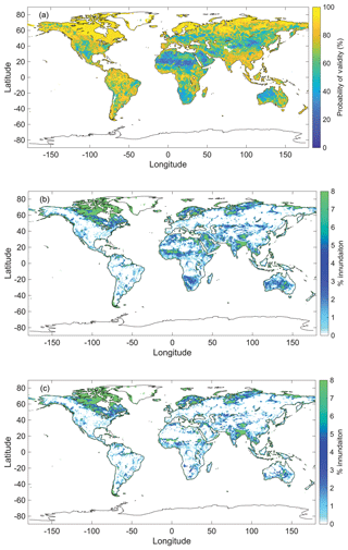
Figure 1 (a) SWAMPS quality control map. (b) Example of monthly SWAMPS measurements for August 2007. (c) Figure 1b after locations less than 50 % probability of validity are removed.

GPCP is available from the National Oceanic & Atmospheric Administration's (NOAA) Earth System Research Laboratory at a $\mathrm{2.5}{}^{\circ }\times \mathrm{2.5}{}^{\circ }$ (approx. 250 km ×250 km) spatial resolution and monthly temporal resolution from January 1979 to present (Adler et al., 2003). GPCP provides global precipitation measurements in mm d⁻¹ (Fig. 2a).

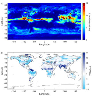
Figure 2 (a) Example of monthly GPCP measurements for August 2007. (b) Example of monthly GRACE total water storage anomaly (TWSA) measurements for August 2007.

GRACE measures the gravity anomaly detected by the orbiting satellites; the JPL (Jet Propulsion Laboratory) GRACE Tellus group processes the anomalies and provides the change in total water storage across the globe (cm) (Fig. 2b). GRACE is available at a $\mathrm{3.0}{}^{\circ }\times \mathrm{3.0}{}^{\circ }$ (approx. 300 km×300 km) spatial resolution and monthly temporal resolution from April 2002 to June 2017 (Watkins et al., 2015; Wiese et al., 2016).

After data acquisition, our preliminary step was to regrid each dataset using linear interpolation to a common $\mathrm{0.5}{}^{\circ }\times \mathrm{0.5}{}^{\circ }$ spatial resolution. Also, we averaged daily surface inundation measurements from SWAMPS to achieve monthly values. The timeframe for this work spanned April 2002 to October 2015, the common period amongst these products. This work involved assessing the viability of a single-linear regression (Eqs. 1 and 2) or multi-linear regression (Eq. 3) model based on GPCP and GRACE to represent surface inundation estimated by SWAMPS. Precipitation and water storage long-term anomalies, a component of the total signal, are known to be globally correlated with a known lag (Humphrey et al., 2016). We utilize full signal in the regressions to ensure levels of orthogonality between precipitation and water storage that avoid collinearity.

$$\begin{array}{}\text{(1)}& {\displaystyle }\mathrm{SWAMPS}=m\left(\mathrm{GPCP}\right)+b\text{(2)}& {\displaystyle }\mathrm{SWAMPS}=m\left(\mathrm{GRACE}\right)+b\text{(3)}& {\displaystyle }\mathrm{SWAMPS}=m_{\mathrm{1}}\left(\mathrm{GPCP}\right)+m_{\mathrm{2}}\left(\mathrm{GRACE}\right)+b\end{array}$$

Using the correlation coefficients (R²) and regression coefficients (slope values; m, m₁, and m₂), we can statistically determine which mechanism will have a stronger influence on surface inundation developments. To further capture the long-term variability across the globe, we utilized each dataset’s climatology.

To develop these climatology datasets, we calculate the long-term monthly average values. The resulting dataset would be a single value at each cell for each month, reflecting the average monthly signal occurring through the historical record. Using the climatology, we can observe the average annual hydrologic cycle anywhere across the globe.

After completing the regressions, multiple grid cells had negative regression coefficients. Negative regression coefficients are of concern because it should generally be impossible to have an inverse relationship between surface inundation and precipitation or groundwater storage. In most cases, time lags between forcing and response (for example, a high TWSA due to snow which only manifests as surface water 3 months later) are responsible for negative regression coefficients within the regressions and applying optimal correlations corrected for time lag improved our statistical strengths. We conducted iterative cross-correlations between TWSA and inundation and between precipitation and inundation to statistically determine the most appropriate time lag correction at each cell location across the globe (Fig. 4). We applied two time lag thresholds: 0 to 5 months and 0 to 11 months. Time lag corrections occur at each grid cell, which shifts the climatology signal of GRACE or GPCP within the phase of SWAMPS.

Figure 3 Methodology flowchart.

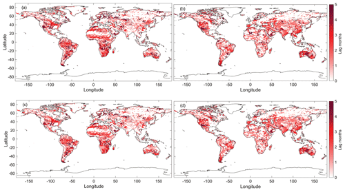
Figure 4 Maps display the number of months between the SWAMPS, GRACE, and GPCP signal that were statistically determined by cross-correlations. (a) GPCP lag map with a time threshold of 0 to 11 months. (b) GRACE lag map with a time threshold of 0 to 11 months. (c) GPCP lag map with a time threshold of 0 to 5 months. (d) GRACE lag map with a time threshold of 0 to 5 months.

The final step in preprocessing the datasets is the removal of low-quality data from the SWAMPS dataset. Schroeder et al. (2014a), issued a quality control (QC) map for the SWAMPS dataset (Fig. 1a), and thus we set the quality threshold at 50 % confidence or higher. As previously stated, desert regions (i.e., the Sahara, southern Africa, and western Australia) and snow-dominated regions (i.e., the Rocky Mountains and central Asia) have poor reliability in measurements, likely due to erroneous reflectivity, and are largely filtered out from the study domain (Fig. 1b and c).

In total, nine regression models were validated by calculating surface inundation and comparison to the SWAMPS dataset. Pearson’s R², the root mean squared error (RMSE), and a ratio between R² and coverage were used to determine each model’s strength. Coverage is considered the number of SWAMPS grid cells with numerical values within the global coastline; for example, analysis excluded Antarctica and Greenland, because there are no SWAMPS data for these regions. A model with a ratio closer to one describes a stronger model; this ratio is important because it considers maximizing coverage and correlation to observations. In choosing the “best” model, we are considering two things: (1) overall model performance at estimating surface inundation and (2) the global coverage retained. With the final model, historical GRACE and GPCP measurements are used to estimate surface inundation (referred to as modeled surface inundation). A best-fit line is applied to display the relationship between modeled surface inundation and measured SWAMPS data.

After selecting the best model, we assessed model performance on a basin and global scale. Correlation statistics (R² and RMSE) between measured and model climatologies and scatterplots are used to present model performance at four highly studied basins: the Amazon River in South America, Mackenzie River in Canada, Mississippi River in the USA, and Ob River in Russia. The difference between modeled and measured surface inundation highlights locations of over- and underestimations across the global domain. We estimated the root mean squared error between modeled and measured surface inundation for our entire observational period to evaluate our model’s error in estimations across the historical record. Finally, the relative error of SWAMPS was calculated using Eq. (4) to determine the error between modeled and measured SWAMPS relative to measured SWAMPS long-term average (LTA).

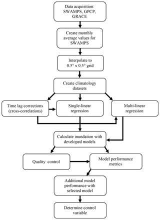
We took the difference between normalized GPCP and GRACE slopes to determine whether groundwater storage or precipitation is relatively more influential in surface inundation developments. These variables were standardized to compare them on the same scale (Eq. 5). Equation (6) is used to compare the standardized slopes. Flows were classified as Horton flows if the value was positive (i.e., precipitation was dominant in runoff generation). Flows were classified as Dunne flows if the value was negative (i.e., TWSA was dominant in runoff generation). Values closer to zero will show that both groundwater storage and precipitation are both equally important in surface inundation developments at that location. The methodology is displayed as a flowchart in Fig. 3 to clarify our process further.

$$\begin{array}{}\text{(4)}& {\displaystyle }\mathrm{Error}\left(\mathit{\%}\right)={\displaystyle \frac{\mathrm{RMSE}}{\mathrm{LTA}}}\text{(5)}& {\displaystyle }\mathrm{Standardized}\mathrm{values}={\displaystyle \frac{x-\mathit{\mu }}{\mathit{\sigma }}}\text{(6)}& {\displaystyle }\mathrm{Control}\mathrm{variable}=\left|\mathrm{GPCP}\mathrm{slope}\right|-\left|\mathrm{GRACE}\mathrm{slope}\right|\end{array}$$

3 Results

Lag maps display the signal lag between SWAMPS and GRACE or SWAMPS and GPCP for 0 to 11 months (Fig. 4a and b) and 0 to 5 months (Fig. 4c and d). Locations in the white represent no lag or no data, and areas in red represent long delays. The color axis range is from 0 to 5 months of lag. We can see minimal differences comparing the lags maps with a time lag correction of 0 to 11 months and 0 to 5 months. The majority of the GRACE and GPCP signal is only out of phase with SWAMPS by at most 5 months. This is statistically supported in Table 1 because R² and RMSE from all scenarios representing 0 to 11 months match their time lag counterpart of 0 to 5 months. We no longer considered all models of 0 to 11 month beyond this point.

Table 1 Model validation results. QC: quality control; RMSE: root mean squared error.

Measured and modeled SWAMPS data are displayed using scatterplots (Fig. 5). The x-axis displays modeled SWAMPS data, while the y-axis represents measured SWAMPS data. These plots reveal global surface inundation measurements from April 2002 to October 2015 without the consideration of quality control (Fig. 5a) and with QC (Fig. 5b). The red line displays the best-fit relationship as determined by MATLAB’s statistical toolbox. We can statistically and visually see the significance of removing locations with less than 50 % QC. The R² increased (0.732 to 0.900), and RMSE decreased (3.830 to 1.890) after QC was applied (Fig. 5). There is a large spread of surface inundation from the model (Fig. 5a), but after masking there is a clear trend line between modeled and measured SWAMPS data (Fig.  5b). Further comparing the validation statistics between single- and multi-linear models, we can see there is not much improvement (Table 1). However, we know that a model with both GRACE and GPCP better represents the world compared to just considering one variable. A multi-linear regression model with a time lag correction improves in both RMSE and R² compared to one without a time lag correction. Therefore, a multi-linear regression model with a time lag correction between 0 to 5 months is the most rigorous model for further analysis.

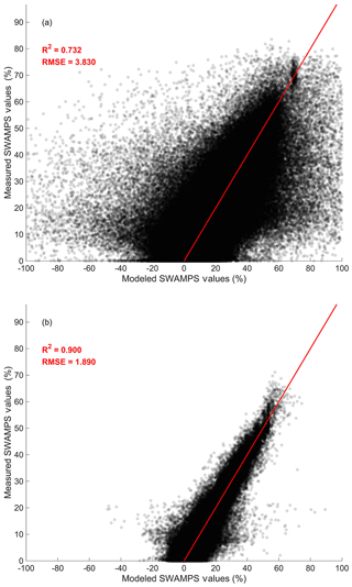
Figure 5 Example of multi-linear regression model validation plots. (a) Measured versus modeled SWAMPS data with a time lag correction of 0 to 5 months. (b) Fig. 5a after locations with less than 50 % probability of validity are removed.

Modeled SWAMPS data using GRACE and GPCP (Fig. 6a) and measured SWAMPS data (Fig. 6b) are displayed with a time lag correction between 0 and 5 months during August 2007. Green locations are reported to have high inundation values, while white spots have low inundation values or no available data. The percent difference between these two maps (Fig. 6c) identifies locations of over- and underestimation. The red, grey, and blue locations represent overestimations, minimal differences, and underestimations, respectively, between modeled and measured inundation. The majority of the domain is grey because the differences between small values of inundation are insignificant. Modeled SWAMPS data have the largest limitations at locations with snow or ice (around the Great Lakes and northern parts of Russia) and in areas that experience seasonal monsoons (Bay of Bengal and west coast of South Africa).

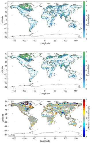
Figure 6 Visual comparison of monthly modeled and measured SWAMPS data. (a) Modeled surface inundation. (b) Measured surface inundation. (c) The absolute difference between modeled and measured surface inundation. Modeled SWAMPS data have a time lag correction of 0 to 5 months.

Regional model performance is assessed through correlation statistics between climatologies and scatterplots for measured and modeled inundation (Fig. 7). The Amazon (Fig. 7a–c), Mackenzie (Fig. 7d–f), Mississippi (Fig. 7g–i), and Ob (Fig. 7j–l) river basins were used for this analysis because their hydrology is well understood and a successful model should maintain its rigor in these significant areas. Blue, red, and green markers (Fig. 7a, d, g, and j) represent randomly selected cell locations along the river; measured and modeled climatologies are represented with solid and dashed lines using the same color scheme (Fig. 7b, e, h, and k); the cell coordinates are in Table 2. Red boxes (Fig. 7a, d, g, and j) outline the cells used in the scatterplots (Fig. 7c, f, i, and l), and their boundary coordinates are also in Table 2. Climatology correlation statistics are in Table 3. Similar to Fig. 5b, the scatterplots relate measured and modeled inundation between April 2002 to October 2015 with QC applied for the cells within the boundaries. The red line displays the best-fit line along with the calculated R². The multi-linear regression model with a time lag correction between 0 and 5 months is used to calculate modeled inundation. The majority of the basins’ domains display strong statistics between the measured and modeled inundation (Table 3). Basins that experience varying snow seasons (Mississippi and Ob) have the largest modeled and measured inundation discrepancies (Fig. 7i and l). These two river basins have the largest spread in modeled versus measured data about the best-fit line and have reduced R² correlations (0.511 and 0.629, respectively). Inadequate data during the snow season limit model performance during these times (no available measurements during winter months, as seen in Fig. 7e and k).

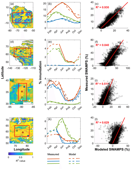
Figure 7 Cells included in scatter plots are outlined by the red boxes, and red, blue, and green dots denote the cell used for measured and modeled climatologies. Modeled inundation has a time lag correction of 0 to 5 months. (a) Amazon map. (b) Amazon measured and modeled climatologies. (c) Amazon scatterplot. (d) Mackenzie map. (e) Mackenzie measured and modeled climatologies. (f) Mackenzie scatterplot. (g) Mississippi map. (h) Mississippi measured and modeled climatologies. (i) Mississippi scatterplot. (j) Ob map. (k) Ob measured and modeled climatologies. (l) Ob scatterplot.

Table 2 Coordinates for basin sites and the boundaries for cells included in the scatterplots.

Table 3 Basin climatology correlation statistics.

To assess global model performance, we calculate the RMSE (Fig. 8a) between the measured and modeled time series at each grid cell. Low RMSE values represent small differences between long-term modeled and measured SWAMPS data, while high RMSE values tell us there are more considerable differences in the signals. Grey represents low error values, while red displays more substantial error. White locations have no value. Long-term surface inundation (Fig. 8b) values range from 0 % to 8 % with high values in green; low values and no values are in white. Figure 8c displays errors (Eq. 4) in our modeled SWAMPS relative to the measured SWAMPS signal. Locations with heavy snow (northern parts of North America, Europe, and central Asia) and regular annual cycles of inundation (India and Amazon) have more significant RMSE values compared to other locations.

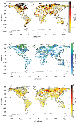
Figure 8 (a) RMSE between modeled and measured SWAMPS data with a time lag correction of 0 to 5 months. (b) Long-term average (LTA) surface inundation. (c) Error relative to the measured SWAMPS signal.

Depending on the global location, either GRACE, GPCP, or both control surface inundation for the model without a time lag correction (Fig. 9a) and for the models with a time lag correction of 0 to 5 months (Fig. 9b) and 0 to 11 months (Fig. 9c). Precipitation dominate locations are red, and groundwater storage controls blue locations. Grey areas represent locations controlled by both GRACE and GPCP. Areas shown in white represent no values. Overall, we determined that both GPCP and GRACE control the majority of surface inundation developments across the world. By taking the standard deviation (σ) of the standardized modeled SWAMPS data (σ=1.04), we determined the percentage of cells controlled by GRACE, GPCP, or both. Cells with a difference less than our calculated standard deviation (−σ) were considered GRACE dominate. Cells with a difference greater than our calculated standard deviation (+σ) were GPCP dominate. Both groundwater- and precipitation-controlled cells have values within ±σ. Using these standards, we found groundwater storage controlled 8.3 % of cells which produced Dunne flows. Precipitation controlled 6.9 % of cells and generated Horton flows. Both variables controlled approximately 84.8 % of cells.

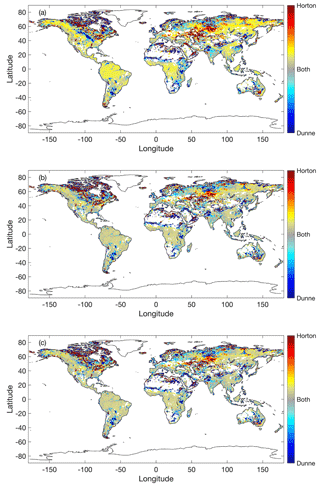
Figure 9 Control variable maps (a) without a time lag correction, (b) with a time lag correction of 0 to 5 months, and (c) with a time lag correction of 0 to 11 months.

Maps with correlation values (Figs. 10, 11a, and b) have a color axis from 0 to 1. Correlations closer to 1, displayed in yellow, represent stronger relationships between SWAMPS and the other dataset(s). Correlations closer to 0, presented in blue, represent weaker relationships between SWAMPS and the other dataset(s). We provided five correlation maps with different inputs: the model with SWAMPS and GRACE without a time lag correction (Fig. 10a), the model with SWAMPS and GPCP without a time lag correction (Fig. 10b), the model with SWAMPS, GRACE, and GPCP without a time lag correction (Figs. 10c and 11a), and the model with SWAMPS, GRACE, and GPCP with a time lag correction of 0 to 5 months (Fig. 11b).

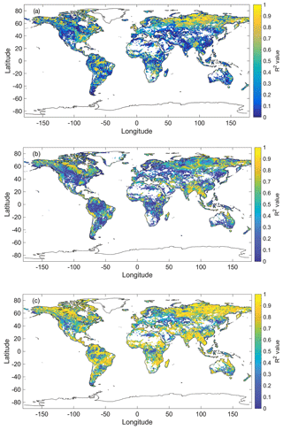
Figure 10 Correlation maps for regression models without a time lag correction. (a) Single-linear regression between SWAMPS and GRACE values. (b) Single-linear regression between SWAMPS and GPCP values. (c) Multi-linear regression between SWAMPS, GRACE, and GPCP values.

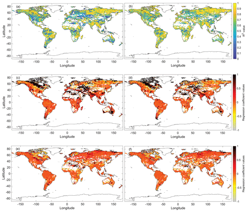
Figure 11 (a) Multi-linear regression correlations without a time lag correction. (b) Multi-linear regression correlations with a time lag correction of 0 to 5 months. (c) GPCP regression coefficients for the model in Fig. 11a. (d) GPCP regression coefficients for the model in Fig. 11b. (e) GRACE regression coefficients for the model in Fig. 11a. (f) GRACE regression coefficients for the model in Fig. 11b.

Correlation maps from the single-linear regressions demonstrate limitations in correlation strengths (Fig. 10a and b). Using GRACE alone, there is a stronger relationship between total water storage and surface inundation within the Amazon River in South America. Precipitation and surface inundation display stronger correlations within the Middle East compared to groundwater storage and surface inundation. It is clear that these single-linear models are capable of describing some surface inundation developments within specific regions but not on a global scale.

There is a significant statistical improvement across the globe when including both groundwater storage and precipitation measurements in estimating surface inundation (Fig. 10c). Locations such as the Amazon, Mississippi, and the Middle East have a higher representation compared to the single-linear models. The time lag adjustment further improves our global correlations. Figure 11a and b display correlations without a time lag correction and with a time lag correction of 0 to 5 months, respectively. We can see visual improvements within the multi-linear regression's correlations east of the Andes and between the Sierra and the Rocky Mountains after the applied time lag correction.

Regression coefficient maps (Fig. 11c–f) have a color axis between −1 and 1. Grey displays negative values, and red represents large values. Regression coefficients for GPCP and GRACE from the model without a time lag correction are shown in Fig. 11c and e, while regression coefficients for GPCP and GRACE from the model with a time lag correction of 0 to 5 months are displayed in Fig. 11d and f, respectively. White locations represent no data. The time lag correction moderates the extreme GPCP slopes around northern Canada and the midwestern region of North America. GRACE slopes around the Great Lakes and Australia also reflect this relationship.

4 Discussion

The surface water formation across the majority of locations within our study domain are controlled almost equally by groundwater storage and precipitation forcings. In our results, for the locations where precipitation has a substantial lag time, groundwater storage tends to have a smaller lag time. The converse is also true, and an inverse relationship follows for a considerable GRACE lag and a slight GPCP lag. Sites such as the Amazon, Middle East, North America, and parts of Asia reflect this pattern. Asia and the Middle East have larger lag times with groundwater storage compared to precipitation, while the Amazon and North America have larger lag times with rainfall compared to groundwater storage.

By emphasizing the climatology, we created a model of inundation based on precipitation and storage that captures and estimates the average seasonal cycle. In areas that are profoundly affected by interannual variability, such as that during El Niño–Southern Oscillation (ENSO) events in locations such as Australia and Africa (Nicholson and Kim, 1997; Power et al., 1999; Ropelewski and Halpert, 1987), our model underestimates these infrequent anomalous fluxes. Heavy snow cover also creates detection issues within the SWAMPS surface water product. The effects of both snow and interannual variability may have influenced RMSE in these locations, and in general, the highest relative error occurs at high elevations and in locations that receive large amounts of snow, especially along the Rocky Mountains (Bales et al., 2006; Berghuijs et al., 2016; Yan et al., 2018). Rain-on-snow events or rapid snowmelt could contribute to a rise in surface inundation without a relative increase in precipitation or groundwater storage. These types of situations are not considered or captured by our model.

No previous literature has attempted to determine inundation developments with TWSA and precipitation measurements rather than just precipitation (Power et al., 1999; Prigent et al., 2007). However, there are studies on the watershed scale that have known control mechanisms. Papa et al. (2010) relate precipitation and river stage height to surface inundation extents within the Amazon. They report precipitation to lead inundation with an influence of snowmelt and glacier melt. We determined precipitation and storage are equally accountable for the inundation developments in the Amazon. Strong correlations between inundation, precipitation, and storage support our result. Papa et al. (2007) relate snowmelt and river discharge to surface inundation within the Ob basin. Maximum inundation is reported to occur between May and June with little to no lag between river discharge and maximum inundation. We report inundation in the Ob basin as driven by water storage, and our reported lags (maximum of 1 month) and modeled surface inundation climatology match their results. Temimi et al. (2005) predict flooding in the Mackenzie River basin by relating river discharge to water surface fraction (WSF). The maximum flooding occurs during the spring when the snowpack melts and ice jams drive flooding. We report inundation developments to be controlled by both water storage and precipitation, and the basin’s modeled climatology reflects the same peak season.

Time lags between inundation and other variables have been well studied in hydrology (Hamilton et al., 2002; Power et al., 1999; Prigent et al., 2007). Our reported precipitation time lags show similarity with those reported by Prigent et al. (2007) in the Amazon and South America. Instead of GRACE observations, Hamilton et al. (2002) correlated river stage observations to inundated areas. For the Roraima and Pantanal floodplains in South America, they report time lags between river stage and inundation of 1 and 1.5 months. We report the lags for those areas to be 2 months. Their use of the nearest river stage station and 0.25^∘ cells of the Scanning Multichannel Microwave Radiometer (SMMR) dataset compared to the 0.5^∘ cells of GRACE may account for this difference.

Our modeled inundation generally overestimated locations with low surface inundation values. Areas along the Rocky Mountains, northern parts of Russia, and Asia all experienced overestimations. Other studies on surface inundation have also reported overestimations at locations with low inundation values (Prigent et al., 2007; Ticehurst et al., 2014). Issues such as cloud coverage, fire scars, heavily snowed areas, and large variation in topography could contribute to these overestimations.

5 Conclusions

This work relates global surface inundation developments to measurements of total water storage and precipitation using NASA remote sensing observations. The novelty of this work is the combined application of the GRACE, GPCP, and SWAMPS data products to study and classify runoff generation mechanisms. We determine a majority of the global surface inundation developments to be equally controlled by total water storage and precipitation. Our methods have the most significant errors at locations with low values of inundation, which agrees with the current literature. Remote sensing has provided novel approaches to study general hydrology concepts on a global scale and holds much promise to further study phenomena in areas with limited in situ data.