the Creative Commons Attribution 4.0 License.
the Creative Commons Attribution 4.0 License.
 | 24 Mar 2020
Reconstructing the 2015 Salgar flash flood using radar retrievals and a conceptual modeling framework in an ungauged basin
Carlos D. Hoyos
Jaime I. Vélez
Esneider Zapata
On 18 May 2015, a severe rainfall event triggered a flash flood in the municipality of Salgar, located in the northwestern Colombian Andes. This work aims to reconstruct the main hydrological features of the flash flood to better understand the processes modulating the occurrence of the event. Radar quantitative precipitation estimates (QPEs), satellite information, and post-event field visits are used to reconstruct the Salgar flash flood, in an ungauged basin, addressing the relationship among rainfall spatiotemporal structure, soil moisture, and runoff generation during successive rainfall events by using a conceptual modeling framework including landslide and hydraulic submodels. The hydrological model includes virtual tracers to explore the role of runoff and subsurface flow and the relative importance of convective and stratiform precipitation in flash flood generation. Despite potential shortcomings due to the lack of data, the modeling results allow an assessment of the impact of the interactions between runoff, subsurface flow, and convective–stratiform rainfall on the short-term hydrological mechanisms leading to the flash flood event. The overall methodology reproduces the magnitude and timing of the La Liboriana flash flood peak discharge considerably well, as well as the areas of landslide occurrence and flood spots, with limitations due to the spatial resolution of the available digital elevation model. Simulation results indicate that the flash flood and regional landslide features were strongly influenced by the antecedent rainfall, which was associated with a northeasterly stratiform event. The latter recharged the gravitational and capillary storages within the model, moistening the entire basin before the occurrence of the flash flood event and impacting the subsurface–runoff partitioning during the flash flood event. Evidence suggests that the spatial structure of the rainfall is at least as important as the geomorphological features of the basin in regulating the occurrence of flash flood events.
- Article
(10103 KB) - Full-text XML
- BibTeX
- EndNote


Flash floods are regarded as one of the most destructive hydrological hazards, resulting in considerable loss of human life and high costs due to infrastructure damage (Roux et al., 2011; Gruntfest and Handmer, 2001). Among all different types of floods, Jonkman (2005) shows that flash floods result in the highest average mortality rate per event (3.62 %), almost 10 times larger than the mortality rate for river floods. Flash floods are usually described as rapidly rising water-level events occurring in steep streams and rivers, associated with short-term, very intense convective precipitation systems or orographically forced rainfall events over highly saturated land surfaces and steep terrains (Šálek et al., 2006; Llasat et al., 2016; Douinot et al., 2016). Convective precipitation episodes often feature high intensity, short duration, and relatively reduced spatial coverage (Houze, 2004).
Several authors have assessed the role of the geological and geomorphological features of the catchment, soil type, soil moisture conditions, and spatiotemporal structure of rainfall in flash flood occurrence, identifying the leading causative mechanisms of this hazard (Merz and Blöschl, 2003). Adamovic et al. (2016) and Vannier et al. (2016) related the flash floods governing processes to the geological properties of the basins, with mixed results. Wu and Sidle (1995) emphasized the role of the topography, ground cover, and groundwater in the occurrence of shallow landslides and associated debris flows. Many authors have assessed the influence of hills and stream slopes, suggesting the slopes of the hills are significantly more important for flash flood occurrence and magnitude than the slope of the stream (Šálek et al., 2006; Roux et al., 2011; Yatheendradas et al., 2008; Younis et al., 2008). Rodriguez-Blanco et al. (2012) analyzed flash flood episodes in Spain and determined that antecedent soil moisture conditions play a significant role in runoff production. Castillo et al. (2003) also suggested a significant correlation between flash flood magnitude and the antecedent moisture conditions. Aronica et al. (2012) used spatial and statistical analysis to reconstruct landslides and deposits, finding a connection between flash flood occurrence and soil moisture antecedent conditions.
The fact that small basins are more prone to flash floods (Wagener et al., 2007) makes their measurement difficult and, consequently, their understanding and their prediction (Hardy et al., 2016; Ruiz-Villanueva et al., 2013; Yamanaka and Ma, 2017; Borga et al., 2011; Marra et al., 2017). The local rainfall storm events related to flash floods require that high spatiotemporal resolution be characterized (Norbiato et al., 2008). Some authors follow a climatological approximation to assess the recurrence of flash floods in particular regions, focusing on the atmospheric causative mechanisms. For example, Kahana et al. (2002) examined the extent to which floods in the Negev Desert are the outcome of climatological synoptic-scale features, finding that about 80 % of the events can be linked to distinct synoptic conditions occurring days prior to the flood events. Schumacher and Johnson (2005) studied extreme rain events associated with flash flooding in the United States over a 3-year period, using the national radar reflectivity composite data. They found that 65 % of the total number of flash floods are associated with mesoscale convective systems (MCSs), with two recurrent patterns of organization: the existence of training convective elements and the generation of quasi-stationary areas of convection with stratiform rainfall downstream. Fragoso et al. (2012) analyzed storm characteristics and rainfall conditions for flash flood occurrence at Madeira (Portugal), and their results suggest an essential role of global climate patterns (North Atlantic Oscillation – NAO – forcing) and local forcing (orographic features) in the triggering of such events. Implicitly, these studies and all the others available in the peer-reviewed literature point to the need for local and regional high-quality spatiotemporal rainfall data. Berne and Krajewski (2013) highlighted the need to incorporate high-resolution weather radar information, even with some limitations, in flash flood hydrology.
The topography of Colombia is characterized by three branches of the Andes crossing the country south-to-north, generating a mixture of landscapes from high snow-capped mountains, vast highland plateaus, and deep canyons to wide valleys, making some regions highly prone to flash flood occurrence. The likelihood of flash flood occurrence in Colombia is also high due to the spatiotemporal behavior of the Intertropical Convergence Zone and the direction of the near-surface moist air flow leading to orographic enhancement of convective cores (Poveda et al., 2007). In the last decade, there have been several widespread and localized flash flood events in Colombia associated with climatological features and the local intensification of rainfall events. According to estimates by the Comisión Económica para América Latina y el Caribe, the 2010–2011 La Niña event alone triggered 1233 flooding events and 778 mass removal processes in Colombia, with more than 3 million people affected and damages estimated at more than USD 6.5 billion.
Since the 2010 widespread disaster, several isolated events have occurred in the country, with devastating consequences. The present paper focuses on studying the processes triggering a flash flood in La Liboriana basin, a 56 km2 basin located in the western range of the Colombian Andes, as a result of consecutive rainfall storms that took place between 15 and 18 May 2015. The resulting flash flood dramatically affected the region, causing more than 100 casualties, affecting several buildings and critical infrastructure, and resulting in a total reconstruction cost estimated at COP 36 000 million (about USD 12.5 million considering the 2018 exchange rate), which corresponds to 3 times the annual income of the municipality. Figure 1 shows an example of infrastructure damage and changes in the basin's main channel as a result of the flash flood event, showing considerable river margin and bed erosion. Despite the data scarcity, including of discharge measurements, the analysis of the successive rainfall events triggering the Salgar flash flood provides an interesting case study for assessing the mechanisms that depend on the soil moisture conditions and rainfall distribution.
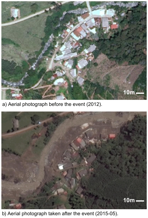
Figure 1Example of infrastructure damage as a result of the La Liboriana flash flood event on 18 May 2015. (a) Aerial photograph taken before the event (2012), during a mission of the Department of Antioquia's government, and (b) a satellite image after the event (courtesy of CNES/Airbus via © Google Earth). The images show the destruction of most houses in that particular community, a bridge over La Liboriana, and the main road. All of the houses shown in the 2015 image had to be either demolished or structurally repaired. The images also show changes in the delineation of the main channel as well as considerable erosion in the river margins.
La Liboriana is a typical case of an ungauged basin (Sivapalan et al., 2003; Seibert and Beven, 2009; Beven, 2007; Bonell et al., 2006; Yamanaka and Ma, 2017), without any detailed records of soils or land use, topographic maps or high-resolution digital elevation models (DEMs), and scarce hydro-meteorological data. According to Blöschl et al. (2012), there are three general strategies for using models under these conditions. The first strategy is to obtain the required model parameters from the historical basin behavior and the morphological characteristics of the basin. This strategy often leads to low model performance (Duan et al., 2006). The second approach is to inherit the hydrological model calibration from a neighboring gauged watershed, which in this case does not exist. The third method is to parameterize the model based on proxy variables, such as hydraulic information obtained during field visits. In the case of the 2015 La Liboriana basin flash flood, there are no previous historical streamflow records nor records from a neighboring watershed; thus, we followed the third approach. We use precipitation information derived from radar, satellite and aerial images, in addition to post-event field visits, to reconstruct the Salgar flash flood event. This study addresses two broad hydrological issues. The first issue consists in exploring the relationship between rainfall spatiotemporal structure (Llasat et al., 2016; Fragoso et al., 2012), soil moisture and runoff generation (Penna et al., 2011; Tramblay et al., 2012; Garambois et al., 2013) during the successive rainfall events and the second one in proposing a simplified hydrological modeling scheme, including landslide and hydraulic submodels, to assess the potential occurrence of flash flood events.
We use the WMF (Watershed Modeling Framework), which includes a variation of the TETIS hydrological model (Vélez, 2001; Francés et al., 2007), modified to include a shallow landslide submodel, and a floodplain submodel called HydroFlash. The TETIS model is a cell-distributed conceptual hydrological model that uses storage tanks and the kinematic wave approximation to simulate the most relevant processes in the basin. The landslide submodel is a stability model that classifies cells into unconditionally stable, unconditionally unstable, and conditionally stable depending on geomorphology; conditionally stable cells are further classified as stable or unstable based in their variable water content (Aristizábal et al., 2016). HydroFlash is a low-cost 1-D model that estimates the cross-sectional filled area at all time steps on the basis of the liquid discharge and the sediment transport. In addition, the TETIS model was modified to include four virtual tracers to separately explore the role of runoff and subsurface flow as well as the relative importance of convective and stratiform precipitation in flash flood generation. The assessment of the interactions between runoff, subsurface flow, and convective–stratiform rainfall allows a better understanding of the short-term hydrological mechanisms leading to the flash flood event.
The document is structured as follows. Section 2 describes in more detail the region of study, La Liboriana basin, including geomorphological and climatological characteristics of the basin and the information sources used in this assessment. Section 3 presents a description of the overall methodology and the TETIS model, including flow separation, and the shallow landslide and HydroFlash submodels. Section 4 describes the main results of the study, including model validation and sensitivity analysis, and presents results from the landslide and HydroFlash submodels. Section 5 includes a discussion on the role of the rainfall structure in the flash flood reconstruction. Finally, the conclusions are presented in Sect. 6.
2.1 Catchment description
The urban area of the municipality of Salgar is located near the outlet of La Liboriana basin, a small (56 km2) tropical watershed located in the westernmost range of Colombia's Andes (Fig. 2). By 2015, Salgar counted 17 400 inhabitants, including 8800 residing in the urban area. La Liboriana basin joins the El Barroso river basin, and both drain to the Cauca River.
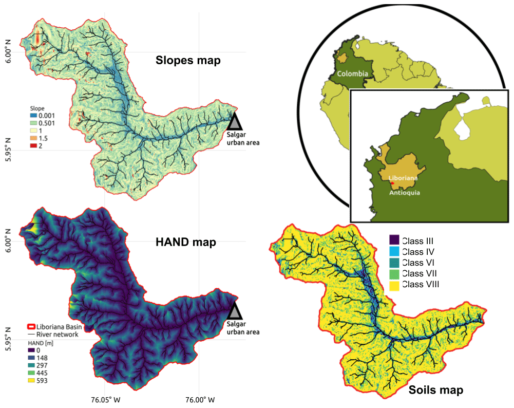
Figure 2Geographical context of the Liboriana basin, located in Colombia, in the Department of Antioquia. The panels include the map of slopes, the height above the nearest drainage (HAND), and the soil type map. The HAND values were estimated using a 12.7 m resolution digital elevation model (DEM). Low HAND values correspond to areas prone to flooding. Note that the soil type map is an extrapolation of the soil properties as a function of slope.
The availability of the ALOS-PALSAR DEM (ASF, 2011), with a resolution of 12.7 m, allows us to estimate the main geomorphological features of the basin. The average slope of La Liboriana is 57.6 %, and the basin longitude and perimeter are 13.5 and 57.8 km, respectively. The Strahler–Horton order of the main stream is 5, and its longitude and slope are 18.1 km and 8.1 %, respectively. The highest elevation of the watershed (Cerro Plateado) reaches 3609 m a.s.l. (above sea level), while the outlet of the basin is at 1316 m a.s.l. The 99th slope percentile of order 1 streams is 78 %. For streams of order 2 to 5, the 99th slope percentiles are 61 %, 27 %, 18 % and 11%, respectively. Figure 2 shows the spatial distribution of the slopes in the watershed. These features are typical of Andean mountainous basins. Geomorphologically, this kind of watershed tends to be prone to the occurrence of flash floods (Lehmann and Or, 2012; Penna et al., 2011; Martín-Vide and Llasat, 2018; Longoni et al., 2016; Ozturk et al., 2018; Khosravi et al., 2018; Marchi et al., 2016; Bisht et al., 2018).
At the subbasin scale, La Liboriana exhibits a vast range of slopes and altitude differences. Figure 2 shows the height above the nearest drainage (HAND) model (Rennó et al., 2008) for La Liboriana. The HAND calculates the relative height difference between cell i and its nearest streamflow cell j. La Liboriana HAND exhibits values between 500 and 800 m. Near the outlet of the basin, over the banks, there are values close to 0 m. High HAND values in the upper region of the watershed often denote areas of high potential energy, with increased sediment production and frequent shallow landslide occurrence. Banks with low HAND values are more susceptible to flooding and tend to correspond to areas prone to extensive damages caused by extreme events. The social challenges lie in the high vulnerability of Salgar, given the location of the main urban settlement.

Figure 3Aerial overview of La Liboriana basin (source: © Department of Antioquia). The top-right panel presents the entire basin, showing the locations of key regions detailed in the following panels, in zooms 1 to 5. The stream network is also presented, colored by order, from yellow to deep blue corresponding to orders 1 to 5.
Vegetation and land use vary considerably within the basin. Figure 3 shows land use in different regions of the watershed from a 2012 aerial image. In the upper region of the La Liboriana basin, there is dense vegetation (see Zoom 1 in Fig. 3), with a high percentage of the area covered by tropical forests and presence of grass and few crop fields. A portion of the upper watershed is considered a national park. Hillslopes near the divide do not show significant anthropic intervention, most likely due to the steepness of this region. Down the hills and at the bottom of the valley, there are coffee plantations (the primary economic activity of the region) and pastures. Downstream (Fig. 3, Zoom 2), the presence of crops is evident among forest and grass areas. Near the middle of the basin (Fig. 3, Zoom 3), the presence of crops is more obvious, and human settlements and roads start to appear. The watershed exhibits grazing areas and urban development near the river banks. In Fig. 3, the Zoom 4 corresponds to the first affected urban area from upstream to downstream during the flash flood. It is also possible to see a marked presence of crops and some patches of forest. Finally, Zoom 5 shows the main urban area of Salgar surrounded by crops, grass and an important loss of forest coverage.
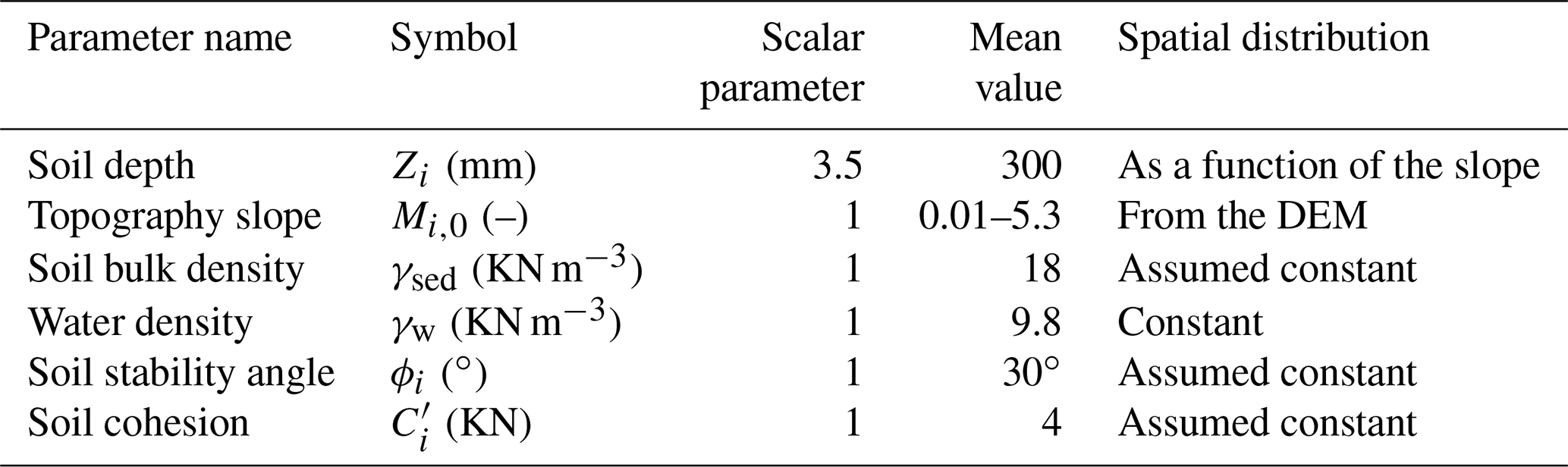
One of the challenges for hydrological modeling and risk management in the country is that soils are not well mapped; the national soil cartography is usually available at a 1:400 000 scale. At this scale, the municipality of Salgar, including La Liboriana basin, corresponds to only one category of soil texture. Osorio (2008), based on field campaign observations and laboratory tests, described La Liboriana soils as well drained with poor retention capacity. Organic material is predominant in the first layer, and clay loam soil predominates within the second layer. The depth of the soil is hillslope dependent, varying from 20 cm to 1 m (Osorio, 2008). Table 1 provides a summary of soil characteristics for five different categories, all as a function of slope. Each soil category has a corresponding depth and a qualitative description of permeability and retention.

2.2 Flash flood post-event observations
We conducted a field campaign a few days after the 18 May flash flood to assess the cross-sectional geometry along the main channel in different sites, including at the outlet of the basin. During the campaign, we measured sectional distances and the surface water speed, at different points of the streamflow. The surface water speed was measured using a hand-held Stalker Pro II velocity radar. We also identified traditional post-event terrain, land cover, vegetation and infrastructure markers to record the approximate level associated with the peak flow during the flash flood. Figure 4 presents the selected cross section used for the estimation of the maximum discharge during the flash flood given its geometrical and hydraulic regularity. The section has a rectangular shape, a width of 4.6 m and a height of 5 m for a total area of 23 m2. A visual inspection of the flooded house around the section, located 4–5 m away from the channel, reveals the presence of mud marks on the walls with heights varying between 0.5 and 1.2 m (see Fig. 4). The area of the section plus the flooded area during the event was estimated to be 37 m2. During the campaign, the surface speeds in the channel varied between 2 and 3 m s−1, for a 3 m3 s−1 discharge. Instrumented basins in the region, with similar characteristics in terms of area and slopes, show peak flow surface water speeds ranging between 5 and 7 m s−1 (see Fig. A1). By assuming an area of 37 m2 and velocities between 5 and 6, we estimate that the flash flood peak flow was between 185 and 222 m3 s−1. Local authorities reported that the peak streamflow reached the urban perimeter after 02:10 LT on 18 May (personal communication during the field visit). Reports state that the peak flow in the most affected community occurred near 02:40 LT1
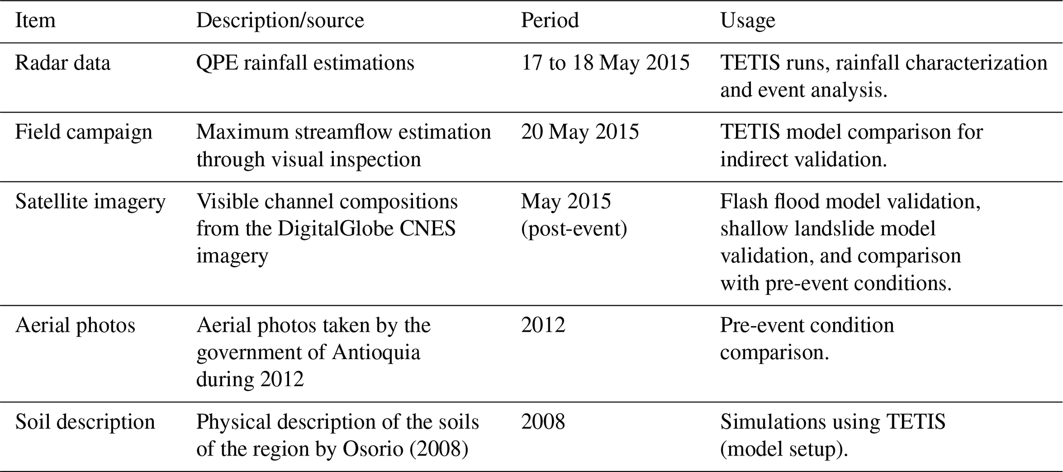
Aerial information before and after the occurrence of the event is relevant to analyze the locations of the landslides and flooded areas. During 2012, the Department of Antioquia conducted a detailed aerial survey of the municipality of Salgar, and a few days after the event, DigitalGlobe and CNES/Airbus made available highly detailed satellite images of the same region. We performed a detailed contrast between both products by using a geographic information system (QGIS), which provided us with information about flooded areas and landslide locations (see Figs. 1 and 16). Field campaign peak flow estimates and aerial imagery are used to validate the results obtained with the TESTIS model.
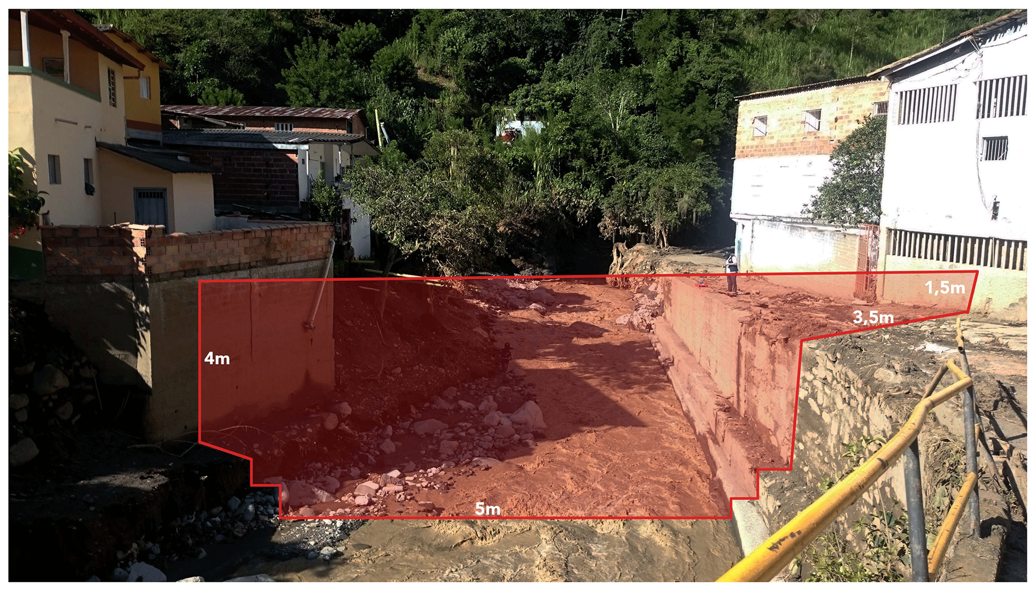
Figure 4Channel cross section showing an example of flooded infrastructure during the flash flood event. The section shows mud marks on the walls of adjacent houses, with heights varying between 0.5 and 1.2 m. The houses in the picture are located 4–5 m away from the channel. The photograph also shows the width of the channel and the total estimated depth during the flash flood. The cross section is downstream from the bridge shown in the picture.
2.3 Rainfall information
The assessment of the 2015 Salgar flash flood event following a hydrological modeling strategy uses a radar-based QPE technique described in Sepúlveda (2016) and Sepúlveda and Hoyos (2017), using radar reflectivity fields, rainfall gauges and disdrometers. The QPE technique uses retrievals from a C-band polarimetric Doppler weather radar operated by the Sistema de Alerta Temprana de Medellín y el Valle de Aburra (SIATA, a local early warning system from a neighboring region, https://siata.gov.co/siata_nuevo, last access: 25 February 2020). The radar is 65 km away from the basin. It has an optimal range in a radius of 120 km for rainfall estimation and a maximum operational range of 240 km for weather detection. The radar operating strategy allows precipitation information to be obtained at a 5 min time step, with a spatial resolution of about 128 m. Despite the distance between the radar and the basin, and the mountains between them, there are no blind spots for the radar. A comparison between the radar QPE estimates and records from two rain gauges installed 3 d after the flash flood event show a correlation for an hourly timescale of 0.65. A detailed description of the rainfall estimation, as well as the overall meteorological conditions that led to the La Liboriana extreme event, are described in a companion paper (Hoyos et al., 2019). Radar retrievals are also used to classify precipitation into convective and stratiform areas following a methodology proposed by Yuter and Houze (1997) and Steiner et al. (1995), based on the intensity and sharpness of the reflectivity peaks. The methodology has been widely used in tropical regions as reported in the review by Houze et al. (2015).
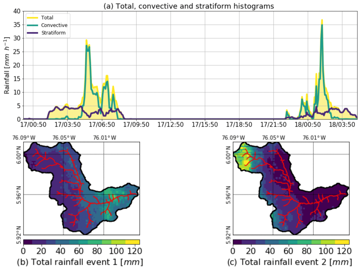
Figure 5(a) Temporal evolution of the convective–stratiform rainfall partitioning during both Events 1 and 2 (precipitation intensity in mm h−1, for 5 min periods). The figure shows the total rainfall (yellow) and the convective (blue) and stratiform (green) portions integrated over La Liboriana basin. (b, c) Spatial distribution of the cumulative rainfall during Events 1 and 2 over La Liboriana basin, respectively.
Between 15 and 18 May 2015, several storms took place over La Liboriana basin. During the night of 17 May, between 02:00 and 09:00 LT (local time), a precipitation event covered almost all of the basin (hereafter referred to as precipitation Event 1). Twenty hours later, between 23:00 LT on 17 May and 02:00 LT on 18 May, two successive extreme convective systems occurred over the basin with the maximum intensity in the upper hills (precipitation Event 2). Event 1 corresponds mainly to a stratiform event with an average precipitation accumulation of 47 mm over the basin. Event 2 corresponds to a moderate average of 38 mm; however, the accumulation exceeded 180 mm over the upper watershed. Hoyos et al. (2019) show that the individual events during May 2015 were not exceptional, the climatological precipitation anomalies were negative to normal, and the synoptic patterns associated with the extreme events were similar to the expected ones for the region. However, the combination of high rainfall accumulation in a 96 h period as a result of successive precipitation events over the basin, followed by a moderate extreme event during 18 May, is unique in the available observational radar record, in particular for the upper part of the basin. Figure 5a presents the temporal evolution of the estimated convective–stratiform rainfall partitioning during both Events 1 and 2. The main difference between both events is the timing of the convective versus stratiform participation within each case. Event 1 started as a stratiform precipitation event moving northeastward, from the Department of Chocó to the Department of Antioquia across the westernmost Andes mountain range. After 3 h of stratiform rainfall, training convective cores move over La Liboriana basin, generating intense precipitation peaks in a 2.5 h period. It is important to note that these cores did not strengthen within La Liboriana basin; these systems formed and intensified over the western hills of Farallones de Citará, draining to the Department of Chocó towards the Atrato River. This is not a minor fact because, as a result of the latter process, the maximum intensity cores did not fall over the steepest hills of La Liboriana basin, but rather near the basin outlet where the slopes are considerably flatter. Figure 5b shows the spatial distribution of cumulative rainfall during Event 1, with the maximum precipitation located toward the bottom third of the basin. Event 2, on the other hand, started as a thunderstorm training event with two convective cores moving from the southeast, followed by the remaining stratiform precipitation. Even though the average cumulative rainfall over the basin was 9 mm less than during Event 1, this event is characterized by orographic intensification within the basin, leading to a more heterogeneous spatial distribution with the highest cumulative precipitation in the steepest portion of the basin (see Fig. 5b).
The data requirements and rainfall preprocessing needed for the overall methodology followed in the reconstruction of the 2015 Salgar flash flood are summarized in Table 2 and are presented in a schematic diagram in Fig. 6.
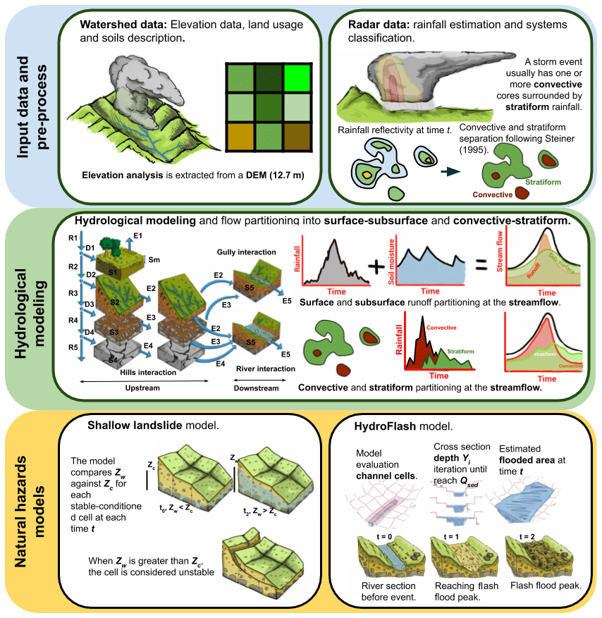
Figure 6Illustrative diagram of the methodology followed in the present study. The top row represents the key input data, specifically a DEM and radar-based QPE as the basis of the modeling framework. The second row represents the conceptual basis of the TETIS model. In each cell, five tanks represent the hydrological processes, including capillary (tank 1), gravitational (tank 2), runoff (tank 3), baseflow (tank 4) and channel storage (tank 5). The state of each tank varies as a function of vertical and lateral flows as shown in the diagram, where the storage is represented by Si and the vertical input by Di, which in turns depends on the vertical flow through tanks Ri. Ei represents the downstream connection between cells and evaporation. The implementation of convective and stratiform rainfall separation and virtual tracers is also portrayed. The implementations of the landslide and HydroFlash submodels are schematized in the bottom row.
3.1 TETIS hydrological model
We used a physically based, distributed hydrological model developed and fully described in Vélez (2001) and Francés et al. (2007). The spatial distribution and the hydrological flow path schema are based on the 12.75 m resolution DEM. In each cell, five tanks represent the hydrological processes, including capillary (tank 1), gravitational (tank 2), runoff (tank 3), baseflow (tank 4) and channel storage tanks (tank 5). The state of each tank varies as a function of vertical and lateral flows as shown in Fig. 6, where the storage is represented by Si (mm) and the vertical input to each tank by Di (mm), which in turns depends on the vertical flow through tanks Ri (mm). Ei (mm) represents the downstream connection between cells, except for tank 1, where E1 represents the evaporation rate.
The original model is modified to improve the representation of the flow processes that occur during flash floods (see Sect. 3.1.1). In addition, two analysis tools of the TETIS results are introduced: virtual tracers tracking convective and stratiform precipitation as well as water paths over or through the soils and a catchment-state analysis by cell grouping (see Fig. 13). The goal is to analyze the spatially distributed response of the watershed to precipitation events of a distinct nature.
3.1.1 Lateral flow modeling modifications
The TETIS model relies on the concept of mass balance where the storage of tank i at the end of the simulation interval Si(t)* (mm) is a function of the storage at the start of the simulation interval Si(t) (mm) and the storage outflow Ei(t) (mm) during the interval t, as follows:
The storage outflow Ei is estimated by transforming the storage Si(t) into an equivalent cross-sectional area Ai (m2), as follows:
where L depends on the model cell width Δx (m), L=Δx for orthogonal flow and for diagonal flow, and Fc (m3 mm−1) is a unit conversion factor that is equal to the area of each cell element Ae (m2) multiplied by 1 m/1000 mm. According to Vélez (2001), Ei changes as a function of Ai, the flow speed vi (m s−1), and the model time step Δt (s), as follows:
The expression for the cross-sectional area at the end of the simulation period Ai(t)* is found by replacing Si(t) in Eq. (2) for Si(t)* and then the resulting expression and Eq. (3) into Eq. (1):
Equation (4) is solved coupled with the equation for the speed vi:
Equation (5) is the generic formulation for the speed used in this work to represent nonlinearities in the relationship between vi and Ai. In the formulation, both β and α change, depending on the type of flow: overland, subsurface, base, and channel flow. The solution for vi is obtained by using the successive substitution method described by Chapra (2012). In the model, we use a 5 min time step, which ensures the stability of the computations. When a solution is reached, Ei is computed using Eq. (3) and Si is updated using Eq. (1).
Nonlinear equations in lateral flows result in a better representation of processes at high resolutions (Beven, 1981; Kirkby and Chorley, 1967). A nonlinear approximation of runoff is presented in Eq. (6). This approximation is a modification of Manning's formula for flow in gullies. According to Foster et al. (1984), ε and e1 are a coefficient and an exponent used to translate the Manning channel concept into multiple small channels or gullies. The values of ε and e1 are 0.5 and 0.64, respectively (Foster et al., 1984). Ai,2 (m2) is the corresponding sectional area obtained from Si,2 by using Eq. (4). In addition, Mi,0 is the slope of the cell, and ni is the Manning coefficient.
The nonlinear Eq. (7) corresponds to an adaptation of the Kubota and Sivapalan (1995) formula for subsurface runoff vi,4, where ki,s is the saturated hydraulic conductivity of cell i and the exponent b is dependent on the soil type, and it is assumed to be equal to 2. Ai,g is the equivalent cross-sectional area of the maximum gravitational storage (Hi,g – mm). Ai,3 is the corresponding sectional area for the gravitational storage (Si,3) obtained by using Eq. (4). There is also return flow from tank 3 to tank 2, when , which represents runoff generation by saturation. In the case of the baseflow, we assume that the speed vi,4 is constant for each cell and depends on the aquifer hydraulic conductivity ki,p (see Eq. 8).
Finally, the streamflow velocity is calculated by using the geomorphological kinematic wave approximation (Vélez, 2001; Francés et al., 2007), in which Λ (km2) represents the upstream area, and Ω and ωi, a regional coefficient and regional exponents, respectively:
An extended discussion of the regional parameters can be found in Vélez (2001). The streamflow speed expression is a version of Eq. (5), this considering that the terms Ω, , , and the exponent ω3 are constant with time.
3.1.2 Tools for spatial analysis of the results: virtual tracers and catchment cell grouping
Virtual tracers are implemented in the model to discriminate the streamflow sources into surface runoff and subsurface flow and to assess the portion of streamflow from convective rainfall and stratiform precipitation, recording the source at each time step and for each cell. The model archives the results of the virtual tracing algorithm at the outlet of the basin and for each reach, enabling us to study the different flow paths and water origins at different spatial scales.
The flow-tracing module operates in tanks 2 (runoff storage) and 3 (subsurface storage). The module marks water once it reaches either of these tanks, and the runoff–subsurface flow percentage is taken into account once the water enters tank 5 (the channel). At this point, the scheme assumes that the water in the channel is well mixed, implying that the flow percentage is constant until new water enters the channel.
With a similar concept, the model also follows convective and stratiform rainfall. For this, at each time step, the model takes into account the rainfall classified as convective or stratiform and assumes that at each particular cell, the precipitation is either entirely convective or entirely stratiform. This assumption could lead to estimation errors at basins represented by coarse cells (low DEM resolution) where convective and stratiform precipitation are likely to coexist. In the present study, the spatial resolution of the DEM is 12.7 m, higher than the resolution of the radar retrievals, so the potential convective and stratiform rainfall concurrence is very low, and it could not be identified using the Steiner et al. (1995) approach.
Additionally, we propose a graphical method to analyze, at the same time, the evolution of multiple hydrological variables in the entire basin. The first step is to classify all the cells within the watershed in a predetermined number of groups according to their localization and the distance to the outlet. The aim is to establish a coherent and robust spatial discretization, thus allowing the concurrent spatiotemporal variability of the different processes to be summarized in 2-D diagrams.
3.1.3 TETIS model calibration
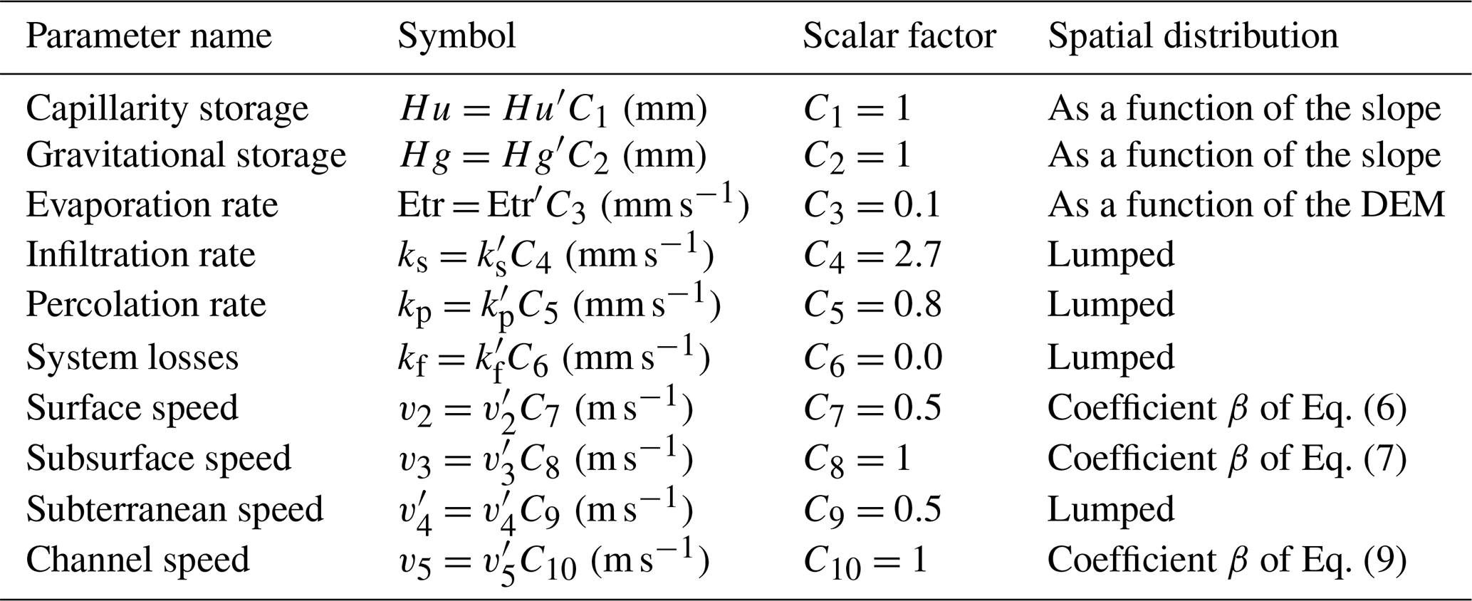
The TETIS model requires a total of 10 parameters. Table 3 includes all the parameters used in the model. The values of the parameters were derived from the soil properties described in Sect. 2. Due to the lack of detailed information in the region, parameters such as the infiltration and percolation rates are assumed to be constant in the entire basin. Other parameters, such as the capillary and gravitational storages, vary as a function of the geomorphological characteristics of the basin such as the elevation and slope. The calibration consists of finding the optimal scaling for each physical parameter, using a constant value for the entire basin (Francés et al., 2007). The model simulation is set to reach a base flow of 3 m3 s−1, a value that corresponds to the discharge measurements during field campaigns days and weeks after the flash flood event, during dry spells. To set the soil wetness initial conditions realistically, the model simulations start 2 d prior to Event 1. Before this period, there were only a couple of weak rainfall events; for this reason, the overall wetness was set to represent dry conditions at the start of the simulation. Table 3 shows the mean value for all of the parameters used in the model and the scalar factor adjusted during the model calibration phase. For the 2015 Salgar flash flood reconstruction, we calibrate the evaporation rate, the infiltration, the percolation, the overland flow speed, and the subterranean flow speed (see Table 3). The values for uncalibrated parameters are inherited from a local watershed with similar characteristics.
Table 3TETIS model parameters. Primed variables correspond to values prior to calibration. Values for the parameters with a scalar factor of 1 are left uncalibrated. Parameters C1 to C6 are not presented in the explanation of the model. C1 modulates the maximum capillary storage and C2 the maximum gravitational storage. C3 to C5 modulate evaporation, infiltration, and percolation rates, respectively. C6 is assumed to be zero, as this variable determines the subterranean system losses. More detail about the calibration parameters is presented in Francés et al. (2007).
3.2 Landslide submodel
The landslide submodel coupled to the TETIS model is proposed by Aristizábal et al. (2016). The stability of each cell is calculated through the assessment of the different stresses applied to the soil matrix. The coupling between TETIS and the landslide submodel is required because the stability of the soil decreases with the porewater pressure (Graham, 1984). The saturated soil depth Zi,w depends on the gravitational storage Si,3(t), the soil wilting point Wi,pwp, and the soil field capacity Wi,fc, as follows:
When Zi,w is greater than the critical depth Zi,c (Eq. 11), failure occurs. The critical saturated depth depends on the shallow soil depth Zi, the soil bulk density γi, the water density γw, the gradient of the slope Mi,0, the soil stability angle ϕi, and the soil cohesion .
Figure 7 describes the variables of the model and the balance of forces considered, and Table 4 presents the required parameters for this model. According to the soil stability definition, the topography and the soil properties, all cells are classified into three classes: unconditionally stable, conditionally stable and unconditionally unstable. In particular, three parameters determine the stability of each cell: (i) residual soil water table Zi,min (Eq. 12), (ii) the maximum soil depth at which a particular soil remains stable Zi,max (Eq. 13), and (iii) the maximum slope at which the soil remains stable Mi,c (Eq. 14).
A cell is unconditionally stable when Zi is smaller than Zi,min or when the cell slope is smaller than Mi,0. On the other hand, a cell is unconditionally unstable when Zi is greater than Zi,max, and finally, a cell is conditionally stable when Zi is between Zi,min and Zi,max. Shallow landslides are calculated at each time step of the hydrological simulation, based on the latter cell class, where the soil stability depends on the storm event, becoming unstable when Zi,w(t) is greater than Zi,c.
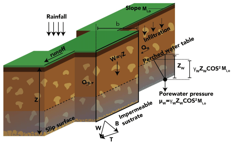
Figure 7Schematic diagram of the landslide submodel. The figure and description are adapted from Aristizábal et al. (2016). QL and QR are the resultant forces on the sides of the slice of soil.
3.3 Floodplain submodel (HydroFlash)
The HydroFlash submodel is designed to interpret the TETIS simulations as floodplain inundations (Fig. 8). For each stream cell and at each time step, the submodel (i) calculates the stream discharge including sediment load (Eqs. 15–20; see Takahashi, 1991) and (ii) determines the inundated cells according to the stream cross profile, the sectional area, and the stream velocities when including the sediment load (Eqs. 19–21, Takahashi, 1991). To determine the discharge including sediment load (Qi,load), a realistic channel width is calculated according to the Leopold (1953) approach as
where Qi corresponds to the streamflow estimated based on a long-term water balance.
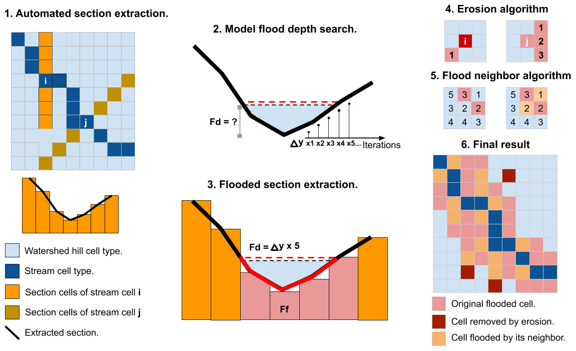
Figure 8Illustrative diagram of the HydroFlash submodel scheme. Step 1: the submodel extracts the cross profile from the network considering the DEM and flow direction. Step 2: based on Eq. (21), the submodel obtains the first approximation of the flash flood streamflow; then, the flood depth and the cross-sectional area are obtained from Eqs. (22) to (21). Step 3: the submodel obtains the flooded portion of the cross section. Step 4: erosion post-process. Step 5: filling post-process. Step 6: the final result for a time step t.
Assuming an infinite sediment and ruble supply, Eqs. (16–(18) are used to deduce, from the channel width Wi, the water level Yi (Eq. 16), the friction velocity vi,fr (Eq. 16, described in Takahashi, 1991), the sediment concentration ci (Eq. 18), and finally the sediment-loaded stream discharge (Eq. 20), as follows:
where vi,sim and Qi,sim are the simulated velocity and streamflow, respectively. Also, ri is the constitutive coefficient of the flow, which summarizes the flow dynamics associated with sediments and colliding particles. The abovementioned relationships depend on two parameters: the maximum sediment concentration (Cmax (–)) and the characteristic diameter of the sediments Di,50 (m). Both terms are assumed to be constant and equal to 0.75 (Obrien, 1988) and 0.138 (Golden and Springer, 2006), respectively.
To determine the inundated cells, the flood depth (Fi,d) and the sectional area of the stream including sediments (Ai,load) are iteratively calculated by reducing the difference between Qi,load and . The channel cross section for cell i, Ei,bed, is defined by the DEM. In each iteration N, the model updates Fi,d with a Δy=0.1 m increase. The cross-sectional area Ai,load is calculated by taking the difference between Fi,d and the elevation of each cell j in the cross section Ei,bed.
The resulting flood maps might include the presence of small isolated flood spots and discontinuities where the flow direction changes from orthogonal to diagonal across or vice versa. We included two post-processing steps to correct these issues by (i) using an image processing erosion algorithm (Serra, 1983) to remove the small and isolated flood spots (step 4 in Fig. 8) and, to solve the flow direction discontinuities, (ii) for each flooded cell the model seeks to inundate the eight neighboring cells: a neighboring cell is also flooded if the altitude of the original flooded cell, plus the flood depth, is higher than its elevation (step 5 in Fig. 8). The image erosion is performed once with a 3-by-3 kernel. An example of the final result for a time step t is shown in step 6 in Fig. 8.
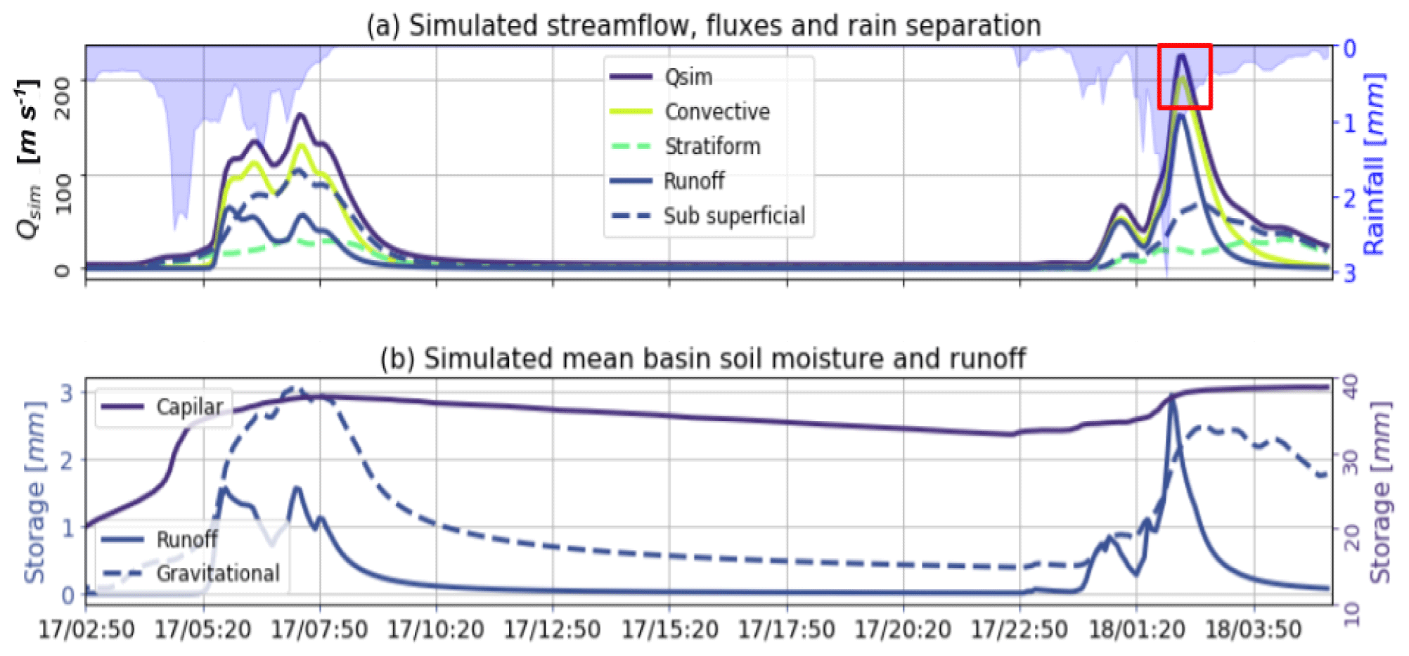
Figure 9Summary of the results from the TETIS hydrological simulation. (a) Simulated streamflow, convective–stratiform-generated discharge discrimination, and runoff and subsurface flow separation. The red square represents the flash flood peak-flow interval that is estimated based on field campaign evidence. (b) Basin-average capillary, runoff and gravitational storages during the simulation period.
The main results of the present study include the reconstruction of the 2015 Salgar flash flood, the assessment of the importance of soil moisture in the hydrological response of the basin, and the evaluation of the relative role of stratiform and convective precipitation cores in the generation of the observed extreme event. This section is based on the analysis of the hydrological simulation as well as the occurrence of shallow landslides and flash floods and their simulation. A comparison of the results from both submodels and the observed landslide scars and flooded spots allows us to evaluate the overall skill of the proposed methodology.
4.1 TETIS validation and sensitivity analysis
Figure 9a presents the results of the hydrological simulation at the outlet of the basin. The simulation shows that Event 1 generates a hydrograph with a peak flow of Qmax=160 m3 s−1. It is important to note that during Event 1, there were no damage or flooding reports by local authorities. Even though this precipitation event did not generate flooding, it set wet conditions in the entire basin before the occurrence of Event 2 (see the purple line in Fig. 9b representing the capillary storage). Additionally, it is clear from the simulation that during the flash flood event, the two successive convective cores over the same region (training convection) generated a peak flow of Qmax=220 m3 s−1, a value that is in the upper range of the estimated streamflow based on post-event field evidence (185–222 m3 s−1). Figure 9a also presents the simulated runoff and subsurface flow separation as well as the convective–stratiform-generated discharge discrimination. The modeling evidence during Event 2 suggests the convective rainfall fraction dominates the hydrograph formation. In both events, convective (stratiform) precipitation appears to be closely related to the simulated runoff (subsurface flow). The simulated subsurface flow is more important in magnitude than the runoff in describing Event 1, while runoff is more relevant for Event 2. Figure 9b presents not only the capillary storage (purple), but also the runoff (continuous blue) and the gravitational storage (dashed blue) temporal variability, as represented by the proposed model. As expected, runoff storage is only nonzero during the storm duration, while gravitational storage increases considerably during rain events, followed by a slow recession. There is an increase in basin-wide capillary storage during Event 1, remaining considerably high during the time leading to the occurrence of Event 2. According to the model simulations, the peak flow occurred at 02:20 LT on 18 May, which is accurate compared to the reports from local authorities (between 02:10 and 02:40 LT), considering all the data limitations.
Figure 10 shows the results of a sensitivity analysis of the hydrological simulation during the second rainfall event, varying the surface speed, infiltration rate, and subsurface speed factors. The aim of the sensitivity analysis is to evaluate the robustness of the overall results, considering the fact that the quality and quantity of some of the watershed information are limited. In the sensitivity analysis, we vary the surface speed factor between 0.01 and 20, the infiltration factor between 0.02 and 20, and the subsurface speed factor between 0.1 and 10. The overall sensitivity results show that the main findings described in the previous paragraphs are, in fact, robust to almost all changes in the mentioned parameters, with the surface runoff associated with convective rainfall controlling the magnitude of the peak discharge during Event 2. The model's highest sensitivity, and hence the largest uncertainty source, appears to be related to the surface speed parameter (Fig. 10a), particularly during the peak flow and the early recession. On the other hand, changes in the infiltration rate factor (Fig. 10b) and subsurface velocity factor (Fig. 10c) are associated with simulation sensitivities smaller than 7 % and 20 % of the peak flow, respectively.

Figure 10Hydrological simulation sensitivity analysis. Similarly to Fig. 9, all the panels show the simulated streamflow (purple) and the runoff (green) and subsurface flow (dashed purple) separation. From top to bottom, the panels show the simulation sensitivity to changes in the (a) surface speed, (b) infiltration rate, and (c) subsurface speed factors.
After the flash flood event, a stream-gauge-level station was installed near the outlet of the basin (see Fig. 2). We use these records to validate the model results without further calibration. Since the observed series correspond to stage-level records, the streamflow estimation is performed following two different approaches. The first approach, the empirical one, consists of subtracting the 10th percentile of the observed stage time series from the observational record and the 10th percentile of the simulated streamflow, from the same series. On the other hand, the second method uses the Manning formula. For this, we consider the geometry of the section in Fig. 4 and the slope from the DEM. Additionally, due to the potential uncertainties, we consider three different Manning values (0.015, 0.02, 0.03). Figure 11 shows the estimated streamflow using the two methods for four different hydrographs during July, August (two events) and December 2015. The simulated magnitudes appear relatively close to the observations, and the peak discharge time is captured skillfully in three of the four cases presented. The discharge values using the “high” Manning number estimation (0.015) are similar to the empirical method. The performance of the model is acceptable (Fig. 11), considering the lack of calibration, the size of the basin, and the magnitude of the recorded events. The results shown include cases where the peak flow was overestimated (Fig. 11c and d) and underestimated (Fig. 11b).
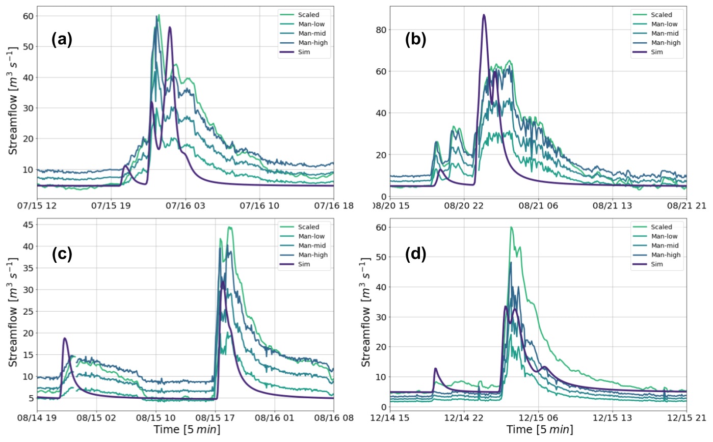
Figure 11Comparison between TETIS simulations and streamflow estimations from a stage-level station installed on a bridge at the outlet of the basin (see Fig. 2).
Figure 12 shows the temporal evolution of discharge during Event 2 in different locations along the watershed's main channel. The upper location corresponds to 15 % of the area of the basin, and the other downstream locations correspond to 52 %, 76 %, and 100 % of the watershed. The difference in the time of the peak discharge between the upper location and the outlet of the basin is around 35 min, which is plausible with travel speeds between 5 and 7 m s−1 and an effective distance of 14 km. In terms of volume, about 737 000 m3 of the total 1 438 000 m3 simulated at the outlet of the basin is generated in the 15 % upstream part of the watershed, corresponding to about half of the total mass. In terms of peak flow, due to the slope and velocity changes, the simulated discharge in the 15 % upstream part of the watershed corresponds to 50 % of the peak discharge at the outlet of the basin.
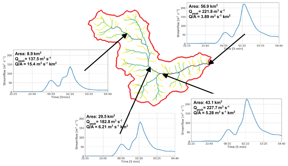
Figure 12Temporal evolution of discharge during Event 2 in different locations along the watershed's main channel. The upper location corresponds to 15 % of the area of the basin, and the other downstream locations correspond to 52 %, 76 %, and 100 % of the watershed, respectively.
4.2 Flash flood processes
Figure 13 presents the proposed 2-D diagrams obtained for the simulation of the La Liboriana basin flash flood using a spatial discretization with 50 groups. Figure 13a includes the evolution of the average rainfall over the basin (black line) and the spatiotemporal evolution of capillary storage (filled isolines) and return flow (colored isolines from white to red) by groups. For the analysis, it is relevant to highlight that higher numbered groups are located away from the outlet of the basin and correspond in this case to considerably steeper slopes. Figure 13b presents the evolution of streamflow at the outlet of the basin (black line) as well as the gravitational storage (filled isolines) and runoff (colored isolines) spatiotemporal evolution. Figure 13 shows variations in the capillary and gravitational storages associated with Event 1 in the higher numbered groups. The capillary storage remains high in almost all the basin until the start of Event 2. According to the conceptualization of the model, the gravitational storage and surface runoff start to interact when the capillary storage is full. In this case, this situation is set up by Event 1. The model runs for Event 2 using dry initial states show no flooding in the results.
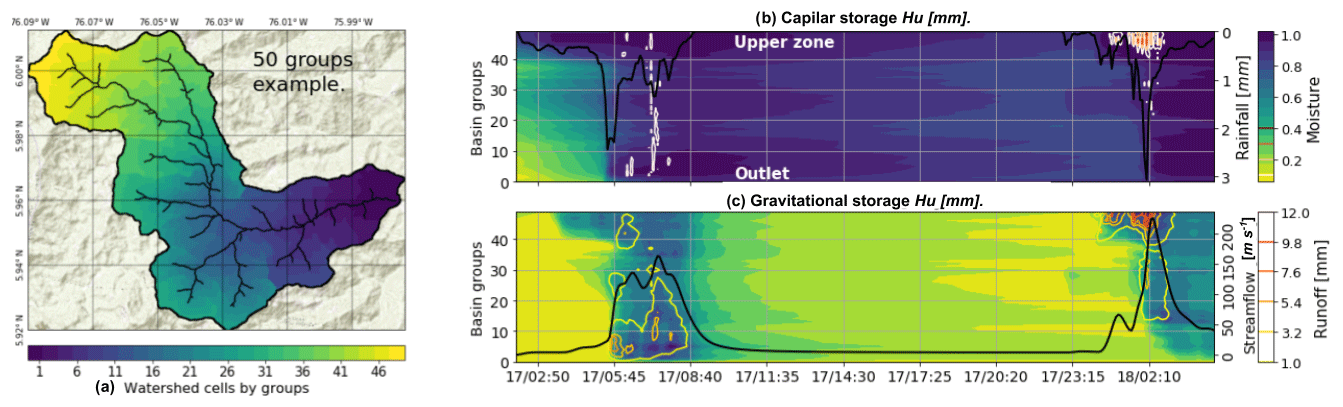
Figure 13(a) Example of watershed grouping as a function of of their localization and distance to the outlet for La Liboriana basin using a 50-group categorization. (b) Simulated capillary moisture (filled green-to-blue contours) and returned flow occurrence (white to red isolines). The black line represents the average rainfall over the basin. (c) Simulated gravitational moisture (filled green-to-blue contours) and runoff (yellow-to-red isolines). The black line represents streamflow at the outlet of the basin. The green-to-blue color bar serves as a reference for capillary moisture and gravitational water content.
The temporal variability of rainfall intensity plays an important role in the hydrograph structure. During Event 1, rainfall accumulated over the basin at a relatively stable rate (Fig. 14a). On the other hand, Event 2 presents a significant increase in rainfall rate in the second half of the life cycle (Fig. 14b). This change in precipitation intensity is associated with a considerable enhancement of the training convective cores due to orographic effects. Events 1 and 2 also exhibit differences in the elapsed time between rainfall occurrence and streamflow increment given the relative timing of stratiform versus convective rainfall (see the gray band in Fig. 14a and b). We compute the elapsed time between the rainfall and the simulated streamflow by measuring the time differences between the lines for the cumulative rainfall and streamflow in Fig. 14. For Event 1, the median elapsed time between rainfall and streamflow (Etp50) is 1.12 h, while for Event 2, Etp50 is 0.79 h. The median elapsed time between the convective portion and the streamflow (Etcp50) in Event 1 is 0.75 and 0.46 in Event 2. The minimum value of the convective elapsed time Etcmin also descends from 0.42 to 0.25 h. On the other hand, there is an increase in median elapsed time between stratiform rainfall and streamflow (Etsp50) from 1.21 to 1.83 h. The observed differences are largely due to the timing of the convective precipitation during each of the events. During Event 1, the convective precipitation occurred near the end of the event, explaining the delayed peak discharge time (see Fig. 5).
According to Fig. 14b for Event 2, the accumulations of streamflow runoff and convective rainfall become similar with the increase in time. This fact highlights the strong control that, in this case, the convective portion has on the runoff, with almost no effect of the stream network filtering out the convective signal, most likely due to the size and the rapid response of the basin. This description, however, only applies for the runoff portion, since the evolution is different when we consider the total simulated streamflow.

Figure 14Accumulated rainfall and streamflow for (a) Event 1 and (b) Event 2. The accumulation is expressed in percentage with respect to the total value in each case. The median elapsed time and minimum elapsed time are estimated between total (Etp50, Etmin), convective (Etcp50, Etcmin), and stratiform (Etsp50, Etsmin) rainfall and the runoff portion of the streamflow. Gray bands correspond to the periods for elapsed time estimation.
4.3 Landslide and flood simulations
Figure 15a presents the observed landslides triggered by Event 2 based on aerial photos and satellite images taken before and after the flash flood. Figure 15b shows, by hills, the map of total unstable cells during the simulation period, and Fig. 15c shows the time series of the number of simulated unstable cells during Event 2 (continuous purple line) and the mean rainfall over the basin (inverse axes, blue line). Calibration of the landslide submodel was performed by finding the maximum overlap between simulated and observed unstable and stable cells, at the same time reducing the overall number of false positives and false negatives. It is important to note that the calibration strategy is not a cell-by-cell modification of the parameters involved, but rather a basin-wide modification of soil properties. A sensitivity analysis of soil parameters is carried out by making small variations of the variables within specified intervals: ϕ between 25 and 32, γ between 17 and 19, C′ between 3.5 and 4.2, and Z between 0.1 and 3 m. The sensitivity analysis suggests that slight variations in the parameter in Z produce the largest changes in the number of unstable cells. Following Table 1, the average soil depth in the basin is only 0.3 m, a value that likely corresponds to underestimation according to the inspections during field visits. For this reason, the results presented in Fig. 15 use a Z map scaled by a calibration factor of 3.5, preserving the spatial dependence on the slope but achieving a more realistic soil depth and better spatial distribution of a landslide occurrence. The model represents the spatial distribution of the areas that are prone to triggering shallow landslides during Event 2 reasonably well, especially in the upper part of the basin, showing a significant density of unstable cells in the hills where slides took place.
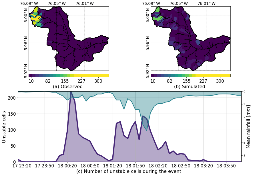
Figure 15(a) Observed landslides triggered by Events 1 and 2. The figure is based on aerial photos and satellite images taken before and after the flash flood event. (b) Map of total unstable cells during the simulation period. (c) Time series of the number of simulated unstable cells during Event 2 (continuous purple line) and mean rainfall over the basin (inverse axes, blue line).
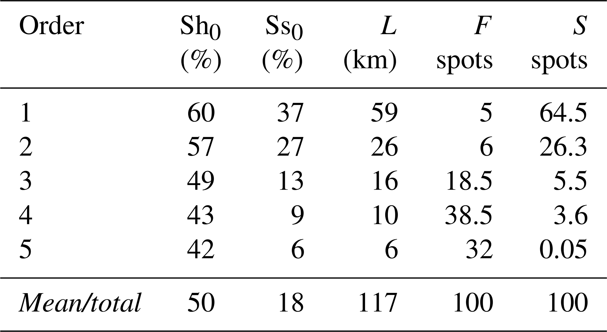
Figure 16 shows the identification of the flood spots at the peak of Event 2 (18 May 2015, 02:00 LT) as simulated using HydroFlash. Figures 16b to f present a detailed view of the results from the outlet of the basin to the upper region. Cases presented in Fig. 16e and f exhibit a satisfactory agreement with observed flood spots (blue shadow). Cases in Fig. 16c and d also show a good approximation, but with minor spatial shifts in some sections. The largest spatial differences are observed in Fig. 16b. At the entrance of the urban zone, the model overestimates the flood spots. The model results indicate that 11 % of flood spots occur at elements of orders 1 and 2, and 18 %, 38 % and 32 % occur at orders 3–5, respectively. Table 5 summarizes the described percentages and the total length of each order. These results also highlight a coherent geomorphological representation of the flooded channels and hills relative to the order.

Figure 16Simulated flood spot at the peak of Event 2 in different locations (image courtesy of CNES/Airbus via © Google Earth). (a) Basin drainage network. White squares correspond to regions of interest highlighted in (b)–(f). The colors of the streams correspond to the Strahler order of the network. (b) Zoom at the outlet of the basin, where an important portion of the human and infrastructure losses took place. (c) Zoom at La Margarita settlement also affected by the flash flood. (d–f) Zoom at key locations along the principal stream. Observed flood spots are shown in blue polygons and model flood spots in red to white grids.
On the morning of 18 May 2015, a flash flood occurred in the steep La Liboriana basin, in the municipality of Salgar, Department of Antioquia, Colombia, leaving more than 100 human casualties, 535 houses destroyed, and significant infrastructure losses. Due to the lack of local information of soil type, land use and real-time hydrometeorological data, the La Liboriana case implies a challenge for flash flood prediction, modeling and, consequently, risk management. The present paper introduces a hydrological model-based approach and an integral graphical analysis tool (an integrated spatiotemporal analysis of rainfall evolution, together with soil storages in the basin) for the following purposes: (1) to simulate and understand the soil–rainfall–discharge processes that led to the 2015 Salgar flash flood and (2) to propose it as a radar QPE-based and modeling-based landslide and flash flood guidance low-cost tool for basins with scarce data and regions with limited resources.
The methodology implies changes and additions to the TETIS-distributed hydrological model, including tracking independently convective and stratiform precipitation within the model as well as keeping track of the runoff and subsurface portions of the streamflow. TETIS was coupled with a shallow landslide submodel and HydroFlash, a 1-D floodplain scheme. The model proposed here indeed allows study of the different hydrological processes relevant to flash flood and landslide occurrence by using different simulation resources, serving as the basis for a better understanding of the overall basin response. Despite the lack of data, the evidence suggests that the results represent, to a large degree, the magnitude of the disaster, considering also that the simulated peak flow is consistent with the peak flow envelope proposed by Gaume et al. (2009) for flash floods. This approach helps to examine the first-order flood-generating mechanisms or causative factors in both time and space, focusing on the most important physical processes (Klemes, 1993; Merz and Blöschl, 2003), potentially allowing the anticipation of flash flooding events, the issue of warnings, and response by risk management entities.
Table 5Channel and flooded cell percentage summary. Sh0 and Ss0 correspond to the mean hill and stream slope, respectively. L corresponds to the total channel length. F spots and S spots correspond to the flooded and slide percentages, respectively.
The evolution of the simulation of Events 1 and 2 shows evidence of remarkable behavioral differences. During Event 1, both gravitational and capillary tanks are filled along and across the basin as a result of the quasi-homogeneous rainfall spatial distribution. Zoccatelli et al. (2011) found similar results for watersheds in Europe with areas ranging between 982 and 52 km2. The return flow is low, and most of the runoff occurs within the first 20 groups (40 % of the watershed closest to the outlet). In the period between both events, there is a recession in the capillary and gravitational storages in the entire basin. Capillary storage decays considerably more slowly than gravitational storage. During Event 2, the flash flood triggering event, the first convective core saturates both capillary and gravitational storages in the upper part of the basin and generates both return flow and significant runoff. Due to soil saturation, the second convective core results mainly in surface runoff. During this event, extreme runoff rates are evident in the upper part of the basin, collocated with the steeper slopes. On the other hand, subsurface flow is more important in magnitude than runoff describing Event 1, while runoff is more relevant for Event 2. The precedent storage and the presence of thunderstorm training profoundly condition the streamflow during Event 2. The overall evidence suggests that precedent capillary moisture in the basin plays an essential role in modulating river discharge. This behavior could be linked to the temporal occurrence and relative importance and timing of the stratiform and convective formations previously described. During the extreme event, when the soils were already wet, the convective rainfall fraction dominated the hydrograph formation. While stratiform rainfall plays an important role moistening the entire basin, convective rainfall generates considerable runoff, leading to flash flooding. Several authors have argued about the role of convective rainfall triggering flash floods (Doswell et al., 1996; Kahana et al., 2002; Schumacher and Johnson, 2005; Delrieu et al., 2005; Šálek et al., 2006; Milelli et al., 2006; Rozalis et al., 2010; Fragoso et al., 2012; Berne and Krajewski, 2013; Gochis et al., 2015; Bruni et al., 2015; Piper et al., 2016; Douinot et al., 2016; Llasat et al., 2016; Baltaci, 2017); however, to our knowledge no other study has tracked convective and stratiform water in a modeling setting to explore their relative role leading to flash flooding.
While convective and stratiform partitioning influence the runoff and subsurface flow separation, the spatial distribution of rainfall relative to watershed network morphometry structure also imposes a condition on the hydrological response of the basin (Douinot et al., 2016). In other words, hydrograph formation is determined not only by the rainfall accumulation or maximum intensity, but also by its spatial structure (Zoccatelli et al., 2011; Douinot et al., 2016). As mentioned before, average rainfall accumulations over the basin for Events 1 and 2 are 47 and 38 mm, respectively. During Events 1 and 2, convective (stratiform) average accumulations are 28 (23) and 17 (14) mm, respectively. The maximum rainfall intensities are relatively similar, with 150 and 180 mm h−1 for Events 1 and 2, respectively, but the location was significantly different. Convective rainfall occurrence at the upper subbasins has significant implications due to geomorphological conditions associated with zero-order subbasins (Sidle et al., 2018). Besides, at Event 2 with a moist soil, the convective portion of the rainfall significantly influences the hydrograph formation. Additionally, when we compare Events 1 and 2, there is an interplay between the rainfall spatial structure and the soil storage capacity. During Event 1, there is almost no saturation, hence runoff production is low, while Event 2 is influenced by the pre-event water and the occurrence of multiple convective systems over the same region. The structure of the rainfall associated with the La Liboriana event and its interaction with the soils highlights the need to consider in more detail the role of orographic rainfall intensification in practical applications such as early warning systems. Evidence suggests the spatial structure of the rainfall is at least as important as the geomorphological features of the basin in regulating the generation of flash flood events.
An integrated spatiotemporal analysis of rainfall evolution, together with soil storages in the basin, is necessary to study the relevance of antecedent conditions and precipitation type, intensity, and location in the generation of flash flood events. Event 1 increased the overall soil moisture with an associated decrease in infiltration rates, similar to the results reported by Marchi et al. (2010), Penna et al. (2011) and Zehe et al. (2010); additionally, low infiltration increased the runoff rates, ultimately affecting the susceptibility of the basin to flash flood occurrence (Wagner et al., 1999; Penna et al., 2011; Tramblay et al., 2012). Due to geomorphological characteristics (see Table 5), water tends to reach the channels in hills of orders 1 and 2 more quickly, and, at the same time, the sediment production and transport in these hills tend to be larger. Order 3 subbasins most likely act as transport elements, with no important energy losses (Table 5), and floods tend to occur at order 4 and 5 subbasins due to the widening of the channel and slope attenuation.
Different authors have focused on trying to understand the general causative factors behind the occurrence of flash floods (Marchi et al., 2010), also suggesting a significant combined role of geomorphology, orography, soil characteristics and local convection. For example, Lehmann and Or (2012), using a shallow landslide model, found an important role of the topography and the rainfall conditions. Turkington et al. (2014) showed how intense locally driven convection is the main meteorological trigger for flash occurrence in the French Alps. Camarasa-Belmonte (2016) showed the important role of rainfall intensity and duration in the shape of the hydrograph, with intense rainfall shortening the response time of the basin and large durations increasing the flood peak. In the Mediterranean region, Boudou et al. (2016) stated that in addition to the rainfall, geomorphological characteristics and antecedent soil conditions are key in the generation of flash flooding.
The landslide submodel presents an overall acceptable performance with limitations in certain regions. In particular, there are some false positives in the middle of the basin. These limitations could be associated with the assumptions and approximations inherent to the submodel, including that it only determines unstable cells by slowly filling the soil matrix with water, which, in this case, given the lack of information, depends on the soil depth derived from the topography, and that the model does not consider instability due to intense rainfall events. The lack of detailed soil depth information could explain the false positive landslides. On the other hand, the relation between landslides and high-intensity rainfall must be explored and included in this kind of model. There is also an apparent contradiction regarding the depth of the soils in the basin: while the values derived from topography appear to work well for the hydrological model, the depth had to be calibrated to obtain a better representation of landslides. There are two possible explanations for the contradiction: (i) that the soils are in fact thicker in the entire basin, but the calibration of the infiltration and percolation rates corrected the hydrological simulations, and (ii) that the landslide submodel is too simplistic or that no other parameters were calibrated, possibly resulting in overcalibration of the soil depth. This is an aspect that needs to be explored further.
The landslide submodel has been used in a nearby watershed with similar characteristics, but with high-quality distributed information (Aristizábal et al., 2016). In that case, the model shows a better performance, which highlights the relevance of the quality of the input data. It is also important to consider that a pinpoint localization of the unstable cells is still considered a hard task, in part due to the small temporal and spatial scale at which landslide processes take place (Aristizábal et al., 2016; Dhakal and Sidle, 2004; Wu and Sidle, 1995).
Similarly, results of the HydroFlash submodel are satisfactory despite the hydraulic oversimplifications and are potentially useful for issuing warnings to the community. From that point of view, it is important to stress that the low computing cost of HydroFlash, different to that of detailed 2-D/3-D hydraulic geomorphological models, makes it possible to be executed in real time coupled with rainfall observations, providing valuable information that, while not 100 % accurate spatially, helps in discriminating to a high degree, for example, which communities need to be evacuated given an extreme event. In addition, the floodplain submodel provides an indirect estimation of the sediment load during extreme events. In the 2015 Salgar simulations, the peak discharge obtained with the hydrological model was 220 m3 s−1; the total streamflow considering the sediment load reached values around 285 m3 s−1, for a Qsed∕Qsim ratio of 1.3. The extra 30 % discharge corresponding to the sediment load is certainly a relevant contribution to the total discharge, with impacts on the floodplain determination. Considering the stream network slope, the simulated ratio is comparable with reports in the literature (e.g., Rickenmann and Koschni, 2010; Chang et al., 2011). The sediment load is mainly constrained by the maximum sediment concentration Cmax and the depth of the flow, suggesting that better information about Cmax could improve the simulation of flood spots. It is important to note that the model was calibrated considering only the water discharge since the uncertainty in the erosion processes and their representation in the model is still significant and the fact that only 1-D processes in the channel are taken into account: The hydrological model relies on water balance. In spite of that, and in order to be on the conservative side for risk management applications, the potential increase in the total discharge associated with the sediment load is considered.
However useful, the evidence in this work only takes into account two successive events; an analysis of more cases and different spatial scales (different basins) would provide robust conclusions in this direction. It is clear that focusing on a single extreme event, rather than on a spectrum of floods, is not conclusive enough (Merz and Blöschl, 2003). The model simulation results suggest it is imperative to study in depth the long-term link between the relative basin and drainage network orientation and the preferred path of precipitation events and its role in defining the frequency of flash flood occurrence. A better understanding of the network-hills-preferential rainfall advection structure could provide information about basins prone to flash floods when information is scarce.
Extreme rainfall events such as the one that triggered the La Liboriana tragedy frequently take place in Colombia and the entire global tropical belt over ungauged basins, often triggering flash floods and debris flows, which endanger vulnerable communities due to poor long-term planning and lack of functional early warning systems. There is a global need for better knowledge and understanding of the hydrological and meteorological conditions that, combined, lead to the manifestation of disasters linked to natural hazards. Such an understanding must result in useful practical applications that improve risk management practices and thus save lives. In the current work, we approach the problem from a hydrological modeling point of view, trying, despite the data limitations and the uncertainty of the results, to shed some light on the first-order processes that modulate the occurrence of flash floods in the region of study.
In the case of the La Liboriana flash flood, radar reflectivity fields were available from a C-Band radar operated by the Early Warning System of Medellín and its metropolitan area, as part of a local risk management strategy. While the municipality of Salgar is located far from Medellín's metropolitan area, the radar is 90 km away from Salgar, and the reflectivity retrievals enable the classification of precipitation fields into convective and stratiform areas, using methodologies widely accepted by the meteorological community. Radar reflectivity also serves as a proxy for precipitation, allowing a quantitative estimation of rainfall fields. This estimation was used together with the TETIS model to assess the different basin-wide processes taking place during the flash-flood-triggering rainfall event. The limitations of the methodology presented in this work do not allow representation of all the detailed small-scale preferential pathways of the water in the watershed, but rather focus on the first-order processes to study the partitioning between runoff versus subsurface flow. Additionally, the model results are used to obtain a conceptual idea about the general processes, but it must be taken into account that the simulations are subject to a calibration process that could lead to erroneous conclusions about the mentioned processes. This consideration could be true even considering that different steps were taken to try to avoid this situation.
The overall model simulation methodology reproduces the estimated magnitude and reported timing of the La Liboriana flash flood discharge peak quite well, showing robustness to changes in the most important model parameters. Simulation results suggest that the soil storage capacity available before the flooding event impacted not only the flood magnitude itself, but also the response time of the catchment, highlighting the role of soil wetness distribution within the basin. The model also reproduces the areas of regional landslide occurrence and flood spot locations satisfactorily. The model simulation results indicate that the flash flood and the regional landslide features were strongly influenced by the observed antecedent rainfall associated with a northwesterly stratiform event that recharged the gravitational and capillary storages in the entire basin. The TETIS model simulation shows that the antecedent event set wet conditions in the entire basin before the occurrence of the flash flood event, governing the streamflow during the latter. The results of the model simulation also suggest that the first of the two successive convective cores (training convective elements) over the same region during the second precipitation event (the flash flood event) saturated both capillary and gravitational storages in the upper part of the basin and generated both return flow and significant runoff. The second convective core resulted mainly in surface runoff spatially collocated with the steeper slopes, generating the kinetic energy needed to produce the La Liboriana flash flood. The overall results also show a good agreement between the simulated flood spots and the observed ones, despite the limitations imposed by the resolution of the DEM used for extracting cross sections and the model oversimplifications.
Results of the landslide submodel and HydroFlash, while satisfactory, are far from perfect, showing significant differences compared to observations. The evidence suggests, by and large, that most of the observed differences are mainly due to the lack of higher spatial resolution DEM, in the case of HydroFlash, and due to the lack of a detailed soil dataset, in the case of the landslide submodel. However, there is also considerable room for improvement in both submodels, including a better representation of non-Newtonian hydraulic processes in HydroFlash and a direct link between landslides and flood spots following, for example, a similar strategy to the one presented in the STEP-TRAMM model (Fan et al., 2017). Notwithstanding the difficulties, the results suggest that the submodel simulations could have been used and should be used in the future for early detection and warning to improve both short- and long-term risk reduction strategies.
Considering all the shortcomings and generalizations, the described model-based approach is potentially useful to assess flood-generating mechanisms and as a tool for policy-makers, not only for short-term decisions in the context of an early warning system, but also as a planning resource for long-term risk management. The results suggest it is possible to use low-cost methodologies such as the one introduced here as a risk management tool in countries and regions with scarce resources.
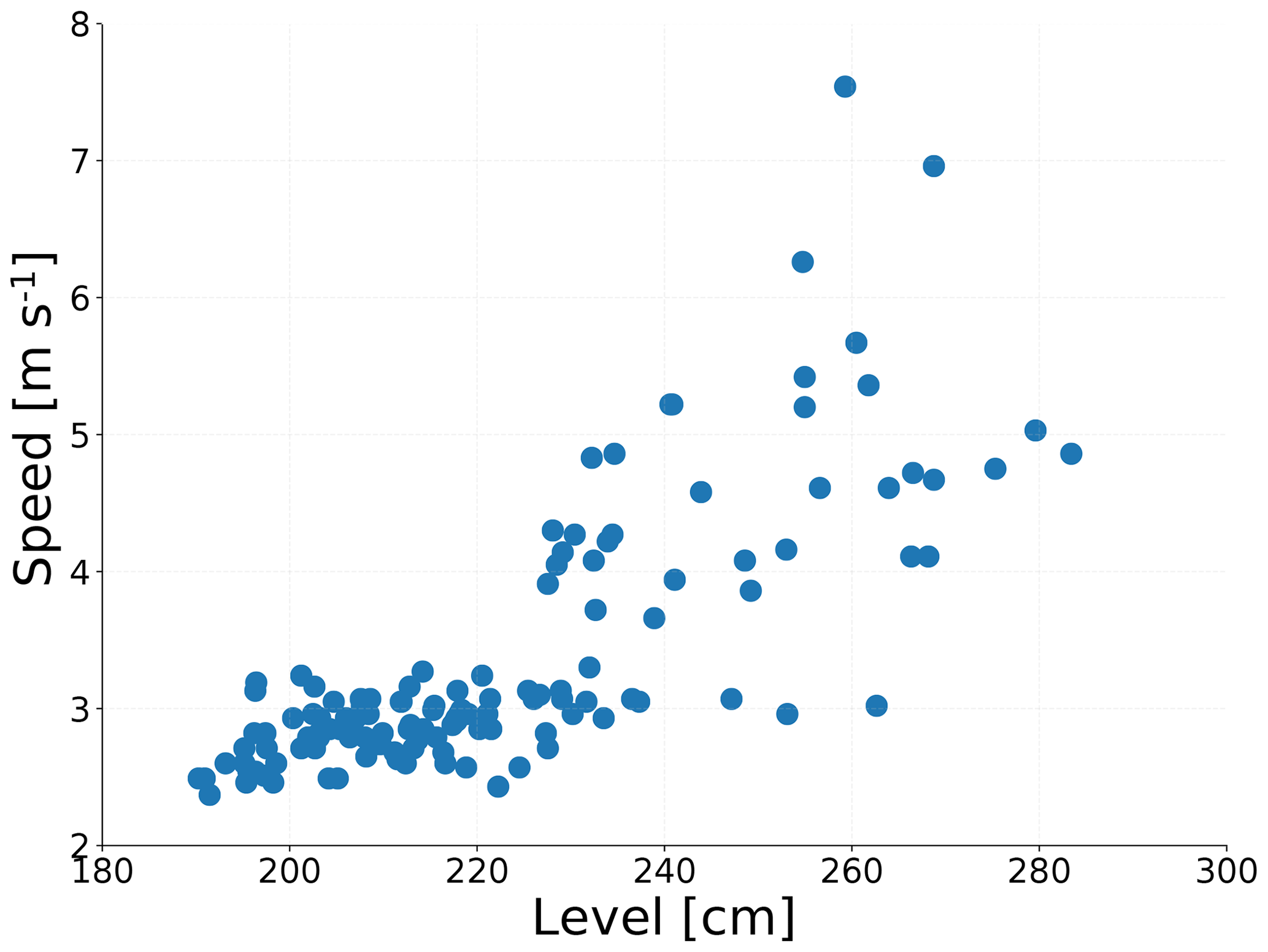
Figure A1Scatter plot of water level (depth) (cm) and surface speed (m s−1) for Doña María basin, located in the Aburrá Valley (basin outlet coordinates: 75.651∘ W, 6.190∘ N). The basin slope is 34.09 %, the area 72.84 km2, and the maximum (minimum) height 2835 m a.s.l. (1562 m a.s.l.).
The data used in this study have been uploaded to a Github and Zenodo repository and are available from https://github.com/nicolas998/SalgarCase (Velasquez, 2020a) and https://doi.org/10.5281/zenodo.3715057 (Velasquez, 2020b), respectively.
NV and CDH conceived the research and prepared the manuscript. JIV gave advice and comments during the process. NV conducted the model developments and hydrological and hazard analysis. EZ and NV developed the flash flood sub-model (hydroFlash).
The authors declare that they have no conflict of interest.
This work was supported by SIATA (Sistema de Alerta Temprana de Medellín y el Valle de Aburrá) funds provided by Area Metropolitana del Valle de Aburrá (AMVA), Municipio de Medellín, Grupo EPM, and ISAGEN under Research and Technology contract CD511, 2017. The Universidad Nacional de Colombia partly funded Nicolás Velásquez under the Facultad de Minas graduate scholarship program. Both authors would like to thank anonymous reviewer no. 1 for the detailed and insightful comments that helped to clarify and highlight the message of this work. Both authors also thank Eric Gaume, reviewer no. 2, for his thoughtful comments.
For the technically inclined reader, the TETIS hydrological model and submodels are written in Fortran 90, and the interface to the model and pre-process and post-process tools are in Python 3.7. The Fortran code is warped to Python using f2py (Peterson, 2009), and it is publicly available under the Watershed Modeling Framework WMF in a web repository (https://github.com/nicolas998/WMF.git, last access: 22 January 2020, GitHub).
This research has been supported by the Area Metropolitana de Medellín y del Valle de Aburrá (AMVA) (grant no. CD511 of 2017).
This paper was edited by Laurent Pfister and reviewed by Eric Gaume and one anonymous referee.
Adamovic, M., Branger, F., Braud, I., and Kralisch, S.: Development of a data-driven semi-distributed hydrological model for regional scale catchments prone to Mediterranean flash floods, J. Hydrol., 541, 173–189, https://doi.org/10.1016/j.jhydrol.2016.03.032, 2016. a
Aristizábal, E., Vélez, J. I., Martínez, H. E., and Jaboyedoff, M.: SHIA_Landslide: a distributed conceptual and physically based model to forecast the temporal and spatial occurrence of shallow landslides triggered by rainfall in tropical and mountainous basins, Landslides, 13, 497–517, https://doi.org/10.1007/s10346-015-0580-7, 2016. a, b, c, d, e
Aronica, G. T., Brigandí, G., and Morey, N.: Flash floods and debris flow in the city area of Messina, north-east part of Sicily, Italy in October 2009: The case of the Giampilieri catchment, Nat. Hazards Earth Syst. Sci., 12, 1295–1309, https://doi.org/10.5194/nhess-12-1295-2012, 2012. a
ASF: Dataset: ASF DAAC 2015, ALOS PALSAR Radiometric Terrain Corrected high res; Includes Material JAXA/METI 2007, https://doi.org/10.5067/Z97HFCNKR6VA, 2011. a
Baltaci, H.: Meteorological analysis of flash floods in Artvin (NE Turkey) on 24 August 2015, Nat. Hazards Earth Syst. Sci., 17, 1221–1230, https://doi.org/10.5194/nhess-17-1221-2017, 2017. a
Berne, A. and Krajewski, W.: Radar for hydrology: Unfulfilled promise or unrecognized potential?, Adv. Water Resour., 51, 357–366, https://doi.org/10.1016/j.advwatres.2012.05.005, 2013. a, b
Beven, K.: Kinematic subsurface stormflow, Water Resour. Res., 17, 1419–1424, https://doi.org/10.1029/WR017i005p01419, 1981. a
Beven, K.: Towards integrated environmental models of everywhere: uncertainty, data and modelling as a learning process, Hydrol. Earth Syst. Sci., 11, 460–467, https://doi.org/10.5194/hess-11-460-2007, 2007. a
Bisht, S., Chaudhry, S., Sharma, S., and Soni, S.: Assessment of flash flood vulnerability zonation through Geospatial technique in high altitude Himalayan watershed, Himachal Pradesh India, Remote Sens. Appl. Soc. Environ., 12, 35–47, https://doi.org/10.1016/j.rsase.2018.09.001, 2018. a
Blöschl, G., Sivapalan, M., Wagener, T., Viglione, A., and Savenije, H.: Runoff Prediction in Ungauged Basins, in: Runoff Prediction in Ungauged Basins: Synthesis across Processes, Places and Scales, edited by: Blöschl, G., Sivapalan, M., Wagener, T., Viglione, A., and Savenije, H., Cambridge University Press, Cambridge, available at: https://www.cambridge.org/core/books/runoff-prediction-in-ungauged-basins/runoff-prediction-in-ungauged-basins/A5DFE99C3CA857127C4C03C6C20032EE (last access: April 2013), 2012. a
Bonell, M., McDonnell, J. J., Scatena, F. N., Seibert, J., Uhlenbrook, S., and van Lanen, H. A. J.: HELPing FRIENDs in PUBs: Charting a course for synergies within international water research programmes in gauged and ungauged basins, Hydrol. Process., 20, 1867–1874, https://doi.org/10.1002/hyp.6196, 2006. a
Borga, M., Anagnostou, E. N., Blöschl, G., and Creutin, J. D.: Flash flood forecasting, warning and risk management: The HYDRATE project, Environ. Sci. Policy, 14, 834–844, https://doi.org/10.1016/j.envsci.2011.05.017, 2011. a
Boudou, M., Lang, M., Vinet, F., and Cœur, D.: Comparative hazard analysis of processes leading to remarkable flash floods (France, 1930–1999), J. Hydrol., 541, 533–552, https://doi.org/10.1016/j.jhydrol.2016.05.032, 2016. a
Bruni, G., Reinoso, R., Van De Giesen, N. C., Clemens, F. H. L. R., and Ten Veldhuis, J. A. E.: On the sensitivity of urban hydrodynamic modelling to rainfall spatial and temporal resolution, Hydrol. Earth Syst. Sci., 19, 691–709, https://doi.org/10.5194/hess-19-691-2015, 2015. a
Camarasa-Belmonte, A. M.: Flash floods in Mediterranean ephemeral streams in Valencia Region (Spain), J. Hydrol., 541, 99–115, https://doi.org/10.1016/j.jhydrol.2016.03.019, 2016. a
Castillo, V. M., Gómez-Plaza, A., and Martínez-Mena, M.: The role of antecedent soil water content in the runoff response of semiarid catchments: A simulation approach, J. Hydrol., 284, 114–130, https://doi.org/10.1016/S0022-1694(03)00264-6, 2003. a
Chang, C.-W., Lin, P.-S., and Tsai, C.-L.: Estimation of sediment volume of debris flow caused by extreme rainfall in Taiwan, Eng. Geol., 123, 83–90, https://doi.org/10.1016/j.enggeo.2011.07.004, 2011. a
Chapra, S. C.: Applied Numerical Methods with MATLAB, 3rd Edn., McGraw-Hill, New York, 2012. a
Delrieu, G., Nicol, J., Yates, E., Kirstetter, P.-E., Creutin, J. D., Anquetin, S., Obled, C., Saulnier, G.-M., Ducrocq, V., Gaume, E., Payrastre, O., Andrieu, H., Ayral, P.-A., Bouvier, C., Neppel, L., Livet, M., Lang, M., du Châtelet, J. P., Walpersdorf, A., and Wobrock, W.: The Catastrophic Flash-Flood Event of 8–9 September 2002 in the Gard Region, France: A First Case Study for the Cévennes–Vivarais Mediterranean Hydrometeorological Observatory, J. Hydrometeorol., 6, 34–52, 2005. a
Dhakal, A. S. and Sidle, R. C.: Distributed simulations of landslides for different rainfall conditions, Hydrol. Process., 18, 757–776, https://doi.org/10.1002/hyp.1365, 2004. a
Doswell, C. A., Brooks, H. E., and Maddox, R. A.: Flash Flood Forecasting: An Ingredients-Based Methodology, Weather Forecast., 11, 560–581, https://doi.org/10.1175/1520-0434(1996)011<0560:FFFAIB>2.0.CO;2, 1996. a
Douinot, A., Roux, H., Garambois, P. A., Larnier, K., Labat, D., and Dartus, D.: Accounting for rainfall systematic spatial variability in flash flood forecasting, J. Hydrol., 541, 359–370, https://doi.org/10.1016/j.jhydrol.2015.08.024, 2016. a, b, c, d
Duan, Q., Schaake, J., Andreassian, V., Franks, S., Goteti, G., Gupta, H., Gusev, Y., Habets, F., Hall, A., Hay, L., Hogue, T., Huang, M., Leavesley, G., Liang, X., Nasonova, O., Noilhan, J., Oudin, L., Sorooshian, S., Wagener, T., and Wood, E.: Model Parameter Estimation Experiment (MOPEX): An overview of science strategy and major results from the second and third workshops, J. Hydrol., 320, 3–17, https://doi.org/10.1016/j.jhydrol.2005.07.031, 2006. a
Fan, L., Lehmann, P., McArdell, B., and Or, D.: Linking rainfall-induced landslides with debris flows runout patterns towards catchment scale hazard assessment, Geomorphology, 280, 1–15, https://doi.org/10.1016/j.geomorph.2016.10.007, 2017. a
Foster, G., Huggins, L., and Meyer, L. D.: A Laboratory Study of Rill Hydraulics: I. Velocity Relationships, Am. Soc. Agricult. Biol. Eng., 3, 0790–0796, https://doi.org/10.13031/2013.32873, 1984. a, b
Fragoso, M., Trigo, R. M., Pinto, J. G., Lopes, S., Lopes, A., Ulbrich, S., and Magro, C.: The 20 February 2010 Madeira flash-floods: Synoptic analysis and extreme rainfall assessment, Nat. Hazards Earth Syst. Sci., 12, 715–730, https://doi.org/10.5194/nhess-12-715-2012, 2012. a, b, c
Francés, F., Vélez, J. I., and Vélez, J. J.: Split-parameter structure for the automatic calibration of distributed hydrological models, J. Hydrol., 332, 226–240, https://doi.org/10.1016/j.jhydrol.2006.06.032, 2007. a, b, c, d, e
Garambois, P. A., Roux, H., Larnier, K., Castaings, W., and Dartus, D.: Characterization of process-oriented hydrologic model behavior with temporal sensitivity analysis for flash floods in Mediterranean catchments, Hydrol. Earth Syst. Sci., 17, 2305–2322, https://doi.org/10.5194/hess-17-2305-2013, 2013. a
Gaume, E., Bain, V., Bernardara, P., Newinger, O., Barbuc, M., Bateman, A., Blaškovičová, L., Blöschl, G., Borga, M., Dumitrescu, A., Daliakopoulos, I., Garcia, J., Irimescu, A., Kohnova, S., Koutroulis, A., Marchi, L., Matreata, S., Medina, V., Preciso, E., Sempere-Torres, D., Stancalie, G., Szolgay, J., Tsanis, I., Velasco, D., and Viglione, A.: A compilation of data on European flash floods, J. Hydrol., 367, 70–78, 2009. a
Gochis, D., Schumacher, R., Friedrich, K., Doesken, N., Kelsch, M., Sun, J., Ikeda, K., Lindsey, D., Wood, A., Dolan, B., Matrosov, S., Newman, A., Mahoney, K., Rutledge, S., Johnson, R., Kucera, P., Kennedy, P., Sempere-Torres, D., Steiner, M., Roberts, R., Wilson, J., Yu, W., Chandrasekar, V., Rasmussen, R., Anderson, A., and Brown, B.: The great Colorado flood of September 2013, B. Am. Meteorol. Soc., 96, 1461–1487, https://doi.org/10.1175/BAMS-D-13-00241.1, 2015. a
Golden, L. A. and Springer, G. S.: Channel geometry, median grain size, and stream power in small mountain streams, Geomorphology, 78, 64–76, https://doi.org/10.1016/j.geomorph.2006.01.031, 2006. a
Graham, J.: Methods of Stability Analysis. Slope Instability, John Wiley and Sons, Chichester, Sussex, England, 1984. a
Gruntfest, E. and Handmer, J.: Coping with Flash Floods, NATO science series. Partnership sub-series 2, Environmental security, Springer Netherlands, available at: https://books.google.com.co/books?id=pwsczTbbY9sC (last access: 25 April 2018), 2001. a
Hardy, J., Gourley, J. J., Kirstetter, P. E., Hong, Y., Kong, F., and Flamig, Z. L.: A method for probabilistic flash flood forecasting, J. Hydrol., 541, 480–494, https://doi.org/10.1016/j.jhydrol.2016.04.007, 2016. a
Houze, R. A.: Mesoscale convective systems, Rev. Geophys., 42, RG4003, https://doi.org/10.1029/2004RG000150, 2004. a
Houze, R. A., Rasmussen, K. L., Zuluaga, M. D., and Brodzik, S. R.: The variable nature of convection in the tropics and subtropics: A legacy of 16 years of the Tropical Rainfall Measuring Mission satellite, Rev. Geophys., 53, 994–1021, https://doi.org/10.1002/2015RG000488, 2015. a
Hoyos, C. D., Ceballos, L. I., Pérez-Carrasquilla, J. S., Sepúlveda, J., López-Zapata, S. M., Zuluaga, M. D., Velásquez, N., Herrera-Mejía, L., Hernández, O., Guzmán-Echavarría, G., and Zapata, M.: Meteorological conditions leading to the 2015 Salgar flash flood: lessons for vulnerable regions in tropical complex terrain, Nat. Hazards Earth Syst. Sci., 19, 2635–2665, https://doi.org/10.5194/nhess-19-2635-2019, 2019. a, b
Jonkman, S.: Global perspectives on loss of human life caused by floods, Nat. Hazards, 34, 151–175, https://doi.org/10.1007/s11069-004-8891-3, 2005. a
Kahana, R., Ziv, B., Enzel, Y., and Dayan, U.: Synoptic climatology of major floods in the Negev Desert, Israel, Int. J. Climatol., 22, 867–882, https://doi.org/10.1002/joc.766, 2002. a, b
Khosravi, K., Pham, B. T., Chapi, K., Shirzadi, A., Shahabi, H., Revhaug, I., Prakash, I., and Tien Bui, D.: A comparative assessment of decision trees algorithms for flash flood susceptibility modeling at Haraz watershed, northern Iran, Sci. Total Environ., 627, 744–755, https://doi.org/10.1016/j.scitotenv.2018.01.266, 2018. a
Kirkby, M. J. and Chorley, R. J.: Throughflow, Overland Flow and Erosion, Int. Assoc. Scient. Hydrol. Bull., 12, 5–21, https://doi.org/10.1080/02626666709493533, 1967. a
Klemes, V.: Probability of extreme hydrometeorological events – A different approach, in: Extreme Hydrological Events: Precipitation, Floods and Droughts, IAHS Publ., IAHS Press, Institute of Hydrology, Wallingford, UK, 1993. a
Kubota, J. and Sivapalan, M.: Towards a Catchment-Scale Model of Subsurface Small-Scale Process-Based Modelling and Runoff Generation Based on Synthesis of Field Studies, Hydrol. Process., 9, 541–554, 1995. a
Lehmann, P. and Or, D.: Hydromechanical triggering of landslides: From progressive local failures to mass release, Water Resour. Res., 48, 1–24, https://doi.org/10.1029/2011WR010947, 2012. a, b
Leopold, L. B. M. T.: The hydraulic geometry of stream channels and some physiographic implications, Geological Survey Professional paper, United States Government Printing office, Washington, 1953. a
Llasat, M. C., Marcos, R., Turco, M., Gilabert, J., and Llasat-Botija, M.: Trends in flash flood events versus convective precipitation in the Mediterranean region: The case of Catalonia, J. Hydrol., 541, 24–37, https://doi.org/10.1016/j.jhydrol.2016.05.040, 2016. a, b, c
Longoni, L., Ivanov, V. I., Brambilla, D., Radice, A., and Papini, M.: Analysis of the temporal and spatial scales of soil erosion and transport in a Mountain Basin, Ital. J. Eng. Geol. Environ., 16, 17–30, https://doi.org/10.4408/IJEGE.2016-02.O-02, 2016. a
Marchi, L., Borga, M., Preciso, E., and Gaume, E.: Characterisation of selected extreme flash floods in Europe and implications for flood risk management, J. Hydrol., 394, 118–133, https://doi.org/10.1016/j.jhydrol.2010.07.017, 2010. a, b
Marchi, L., Cavalli, M., Amponsah, W., Borga, M., and Crema, S.: Upper limits of flash flood stream power in Europe, Geomorphology, 272, 68–77, https://doi.org/10.1016/j.geomorph.2015.11.005, 2016. a
Marra, F., Destro, E., Nikolopoulos, E. I., Zoccatelli, D., Dominique Creutin, J., Guzzetti, F., and Borga, M.: Impact of rainfall spatial aggregation on the identification of debris flow occurrence thresholds, Hydrol. Earth Syst. Sci., 21, 4525–4532, https://doi.org/10.5194/hess-21-4525-2017, 2017. a
Martín-Vide, J. P. and Llasat, M. C.: The 1962 flash flood in the Rubí stream (Barcelona, Spain), J. Hydrol., 566, 441–454, https://doi.org/10.1016/j.jhydrol.2018.09.028, 2018. a
Merz, R. and Blöschl, G.: A process typology of regional floods, Water Resour. Res., 39, 1–20, https://doi.org/10.1029/2002WR001952, 2003. a, b, c
Milelli, M., Llasat, M. C., and Ducrocq, V.: The cases of June 2000, November 2002 and September 2002 as examples of Mediterranean floods, Nat. Hazards Earth Syst. Sci., 6, 271–284, https://doi.org/10.5194/nhess-6-271-2006, 2006. a
Norbiato, D., Borga, M., Degli Esposti, S., Gaume, E., and Anquetin, S.: Flash flood warning based on rainfall thresholds and soil moisture conditions: An assessment for gauged and ungauged basins, J. Hydrol., 362, 274–290, https://doi.org/10.1016/j.jhydrol.2008.08.023, 2008. a
Obrien, J. S. J. P.: Laboratory analysis of mudflow properties, J. Hydrol. Eng., 8, 877–887, 1988. a
Osorio, H. G. A. S.: Unidades de suelo representativas de la zona cafetera de Colombia, Federación de Cafeteros de Colombia, Bogota, Colombia, 2008. a, b, c, d
Ozturk, U., Wendi, D., Crisologo, I., Riemer, A., Agarwal, A., Vogel, K., López-Tarazón, J. A., and Korup, O.: Rare flash floods and debris flows in southern Germany, Sci. Total Environ., 626, 941–952, https://doi.org/10.1016/j.scitotenv.2018.01.172, 2018. a
Penna, D., Tromp-Van Meerveld, H. J., Gobbi, A., Borga, M., and Dalla Fontana, G.: The influence of soil moisture on threshold runoff generation processes in an alpine headwater catchment, Hydrol. Earth Syst. Sci., 15, 689–702, https://doi.org/10.5194/hess-15-689-2011, 2011. a, b, c, d
Peterson, P.: F2PY: a tool for connecting Fortran and Python programs, Int. J. Comput. Sci. Eng., 4, 296–305, https://doi.org/10.1504/IJCSE.2009.029165, 2009. a
Piper, D., Kunz, M., Ehmele, F., Mohr, S., Mühr, B., Kron, A., and Daniell, J.: Exceptional sequence of severe thunderstorms and related flash floods in May and June 2016 in Germany – Part 1: Meteorological background, Nat. Hazards Earth Syst. Sci., 16, 2835–2850, https://doi.org/10.5194/nhess-16-2835-2016, 2016. a
Poveda, G., Vélez, J. I., Mesa, O. J., Cuartas, A., Barco, J., Mantilla, R. I., Mejía, J. F., Hoyos, C. D., Ramírez, J. M., Ceballos, L. I., Zuluaga, M. D., Arias, P. A., Botero, B. A., Montoya, M. I., Giraldo, J. D., and Quevedo, D. I.: Linking Long-Term Water Balances and Statistical Scaling to Estimate River Flows along the Drainage Network of Colombia, J. Hydrol. Eng., 12, 4–13, https://doi.org/10.1061/(ASCE)1084-0699(2007)12:1(4), 2007. a
Rennó, C. D., Nobre, A. D., Cuartas, L. A., Soares, J. V., Hodnett, M. G., Tomasella, J., and Waterloo, M. J.: HAND, a new terrain descriptor using SRTM-DEM: Mapping terra-firme rainforest environments in Amazonia, Remote Sens. Environ., 112, 3469–3481, https://doi.org/10.1016/j.rse.2008.03.018, 2008. a
Rickenmann, D. and Koschni, A.: Sediment loads due to fluvial transport and debris flows during the 2005 flood events in Switzerland, Hydrol. Process., 1007, 993–1007, https://doi.org/10.1002/hyp.7536, 2010. a
Rodriguez-Blanco, M., Taboada-Castro, M., and Taboada-Castro, M.: Rainfall–runoff response and event-based runoff coefficients in a humid area (northwest Spain), Hydrolog. Sci. J., 403, 319–329, https://doi.org/10.1080/02626669509491418, 2012. a
Roux, H., Labat, D., Garambois, P. A., Maubourguet, M. M., Chorda, J., and Dartus, D.: A physically-based parsimonious hydrological model for flash floods in Mediterranean catchments, Nat. Hazards Earth Syst. Sci., 11, 2567–2582, https://doi.org/10.5194/nhess-11-2567-2011, 2011. a, b
Rozalis, S., Morin, E., Yair, Y., and Price, C.: Flash flood prediction using an uncalibrated hydrological model and radar rainfall data in a Mediterranean watershed under changing hydrological conditions, J. Hydrol., 394, 245–255, https://doi.org/10.1016/j.jhydrol.2010.03.021, 2010. a
Ruiz-Villanueva, V., Díez-Herrero, A., Bodoque, J. M., Ballesteros Cánovas, J. A., and Stoffel, M.: Characterisation of flash floods in small ungauged mountain basins of Central Spain using an integrated approach, Catena, 110, 32–43, https://doi.org/10.1016/j.catena.2013.06.015, 2013. a
Šálek, M., Brezková, L., and Novák, P.: The use of radar in hydrological modeling in the Czech Republic – case studies of flash floods, Nat. Hazards Earth Syst. Sci., 6, 229–236, https://doi.org/10.5194/nhess-6-229-2006, 2006. a, b, c
Schumacher, R. S. and Johnson, R. H.: Organization and Environmental Properties of Extreme-Rain-Producing Mesoscale Convective Systems, Mon. Weather Rev., 133, 961–976, https://doi.org/10.1175/MWR2899.1, 2005. a, b
Seibert, J. and Beven, K. J.: Gauging the ungauged basin: how many discharge measurements are needed?, Hydrol. Earth Syst. Sci., 13, 883–892, https://doi.org/10.5194/hess-13-883-2009, 2009. a
Sepúlveda, J.: Estimación cuantitativa de precipitación a partir de la información de Radar Meteorológico delÁrea Metropolitana del Valle de Aburrá, MS thesis, Universidad Nacional de Colombia, Sede Medellín, available at: http://bdigital.unal.edu.co/54581/ (last access: May 2018), 2016. a
Sepúlveda, J. and Hoyos, C. D.: Disdrometer-based C-Band Radar Quantitative Precipitation Estimation (QPE) in a highly complex terrain region in tropical Colombia, in: AGU Fall Meeting Abstracts, December 2017, New Orleans, USA, 2017. a
Serra, J.: Image Analysis and Mathematical Morphology, Academic Press, Inc., Orlando, FL, USA, 1983. a
Sidle, R., Gomi, T., and Tsukamoto, Y.: Discovery of zero-order basins as an important link for progress in hydrogeomorphology, Hydrol. Process., 32, 3059–3065, https://doi.org/10.1002/hyp.13246, 2018. a
Sivapalan, M., Takeuchi, K., Franks, S. W., Gupta, V. K., Karambiri, H., Lakshmi, V., Liang, X., McDonnell, J. J., Mendiondo, E. M., O'Connell, P. E., Oki, T., Pomeroy, J. W., Schertzer, D., Uhlenbrook, S., and Zehe, E.: IAHS Decade on Predictions in Ungauged Basins (PUB), 2003–2012: Shaping an exciting future for the hydrological sciences, Hydrolog. Sci. J., 48, 857–880, 2003. a
Steiner, M., Houze, R. A., and Yuter, S. E.: Climatological Characterization of Three-Dimensional Storm Structure from Operational Radar and Rain Gauge Data, J. Appl. Meteorol., 34, 1978–2007, https://doi.org/10.1175/1520-0450(1995)034<1978:CCOTDS>2.0.CO;2, 1995. a, b
Takahashi, T.: Debris flow, 2nd Edn., Taylor and Francis, London, 1991. a, b, c
Tramblay, Y., Bouaicha, R., Brocca, L., Dorigo, W., Bouvier, C., Camici, S., and Servat, E.: Estimation of antecedent wetness conditions for flood modelling in northern Morocco, Hydrol. Earth Syst. Sci., 16, 4375–4386, https://doi.org/10.5194/hess-16-4375-2012, 2012. a, b
Turkington, T., Ettema, J., Van Westen, C. J., and Breinl, K.: Empirical atmospheric thresholds for debris flows and flash floods in the southern French Alps, Nat. Hazards Earth Syst. Sci., 14, 1517–1530, https://doi.org/10.5194/nhess-14-1517-2014, 2014. a
Vannier, O., Anquetin, S., and Braud, I.: Investigating the role of geology in the hydrological response of Mediterranean catchments prone to flash-floods: Regional modelling study and process understanding, J. Hydrol., 541, 158–172, https://doi.org/10.1016/j.jhydrol.2016.04.001, 2016. a
Velasquez, N.: SalgarCase, GitHub repository, available at: https://github.com/nicolas998/SalgarCase, last access: 2 March 2020a. a
Velasquez, N.: SalgarCase: SalgarData (Version 0.1.1), Zenodo, https://doi.org/10.5281/zenodo.3715057, 2020b. a
Vélez, J.: Desarrollo de un modelo hidrológico conceptual y distribuido orientado a la simulación de crecidas, Tesis doctoral, Universidad Politécnica de Valencia, Valencia, p. 266, 2001. a, b, c, d, e
Wagener, T., Gupta, H., Yatheendradas, S., Goodrich, D., Unkrich, C., and Schaffner, M.: Understanding sources of uncertainty in flash-flood forecasting for semi-arid regions, IAHS Publ., 313, 204–212, 2007. a
Wagner, W., Lemoine, G., and Rott, H.: A method for estimating soil moisture from ERS Scatterometer and soil data, Remote Sens. Environ., 70, 191–207, https://doi.org/10.1016/S0034-4257(99)00036-X, 1999. a
Wu, W. and Sidle, R. C.: A Distributed Slope Stability Model for Steep Forested Basins, Water Resour. Res., 34, 2097–2110, 1995. a, b
Yamanaka, T. and Ma, W.: Runoff prediction in a poorly gauged basin using isotope-calibrated models, J. Hydrol., 544, 567–574, https://doi.org/10.1016/j.jhydrol.2016.12.005, 2017. a, b
Yatheendradas, S., Wagener, T., Gupta, H., Unkrich, C., Goodrich, D., Schaffner, M., and Stewart, A.: Understanding uncertainty in distributed flash flood forecasting for semiarid regions, Water Resour. Res., 44, 1–17, https://doi.org/10.1029/2007WR005940, 2008. a
Younis, J., Anquetin, S., and Thielen, J.: The benefit of high-resolution operational weather forecasts for flash flood warning, Hydrol. Earth Syst. Sci., 12, 1039–1051, https://doi.org/10.5194/hess-12-1039-2008, 2008. a
Yuter, S. E. and Houze, R. A.: Measurements of Raindrop Size Distributions over the Pacific Warm Pool and Implications for Z–R Relations, J. Appl. Meteorol., 36, 847–867, https://doi.org/10.1175/1520-0450(1997)036<0847:MORSDO>2.0.CO;2, 1997. a
Zehe, E., Graeff, T., Morgner, M., Bauer, A., and Bronstert, A.: Plot and field scale soil moisture dynamics and subsurface wetness control on runoff generation in a headwater in the Ore Mountains, Hydrol. Earth Syst. Sci., 14, 873–889, https://doi.org/10.5194/hess-14-873-2010, 2010. a
Zoccatelli, D., Borga, M., Viglione, A., Chirico, G. B., and Blöschl, G.: Spatial moments of catchment rainfall: Rainfall spatial organisation, basin morphology, and flood response, Hydrol. Earth Syst. Sci., 15, 3767–3783, https://doi.org/10.5194/hess-15-3767-2011, 2011. a, b
As reported by the media and the national government: http://www.elcolombiano.com/antioquia/tragedia-en-antioquia-salgar-un-ano-despues-XX4145514 (last access: 15 May 2016), https://caracol.com.co/emisora/2015/12/25/medellin/1451076926_792470.html (last access: 25 December 2015), http://portal.gestiondelriesgo.gov.co/Paginas/Noticias/2015/Antecion-Emergencia-Salgar-Antioquia.aspx (last access: 19 May 2015).