Stream temperature and discharge evolution in Switzerland over the last 50 years: annual and seasonal behaviour

Stream temperature and discharge are key hydrological variables for ecosystem and water resource management and are particularly sensitive to climate warming. Despite the wealth of meteorological and hydrological data, few studies have quantified observed stream temperature trends in the Alps. This study presents a detailed analysis of stream temperature and discharge in 52 catchments in Switzerland, a country covering a wide range of alpine and lowland hydrological regimes. The influence of discharge, precipitation, air temperature, and upstream lakes on stream temperatures and their temporal trends is analysed from multi-decadal to seasonal timescales. Stream temperature has significantly increased over the past 5 decades, with positive trends for all four seasons. The mean trends for the last 20 years are $+\mathrm{0.37}\pm \mathrm{0.11}$ ^∘C per decade for water temperature, resulting from the joint effects of trends in air temperature ($+\mathrm{0.39}\pm \mathrm{0.14}$ ^∘C per decade), discharge ($-\mathrm{10.1}\pm \mathrm{4.6}$ % per decade), and precipitation ($-\mathrm{9.3}\pm \mathrm{3.4}$ % per decade). For a longer time period (1979–2018), the trends are $+\mathrm{0.33}\pm \mathrm{0.03}$ ^∘C per decade for water temperature, +0.46±0.03°C per decade for air temperature, $-\mathrm{3.0}\pm \mathrm{0.5}$ % per decade for discharge, and $-\mathrm{1.3}\pm \mathrm{0.5}$ % per decade for precipitation. Furthermore, we show that snow and glacier melt compensates for air temperature warming trends in a transient way in alpine streams. Lakes, on the contrary, have a strengthening effect on downstream water temperature trends at all elevations. Moreover, the identified stream temperature trends are shown to have critical impacts on ecological and economical temperature thresholds (the spread of fish diseases and the usage of water for industrial cooling), especially in lowland rivers, suggesting that these waterways are becoming more vulnerable to the increasing air temperature forcing. Resilient alpine rivers are expected to become more vulnerable to warming in the near future due to the expected reductions in snow- and glacier-melt inputs. A detailed mathematical framework along with the necessary source code are provided with this paper.

1 Introduction

Water temperature and discharge are recognized as key variables for assessing water quality of freshwater ecosystems in streams and lakes (Poole and Berman, 2001). They influence the metabolic activity of aquatic organisms but also biochemical cycles (e.g. dissolved oxygen and carbon fluxes) of such environments (Stumm and Morgan, 1996; Yvon-Durocher et al., 2010). Water temperature is also a key variable for many industrial sectors, e.g. as cooling water for electricity production or in large buildings, while discharge is an important variable for hydroelectricity production (Schaefli et al., 2019). Water temperature also strongly influences the quality of drinking water by modifying its biochemical properties (Delpla et al., 2009). The ongoing climate change could drastically modify this fragile balance by altering the energy budget and by reducing water availability during warm and dry months of the year. At the global scale, several studies have shown a clear trend over the last few decades with respect to lake surface temperature (Dokulil, 2014; O'Reilly et al., 2015) and stream temperature at various locations (Webb, 1996; Morrison et al., 2002; Hari et al., 2006; Hannah and Garner, 2015; Watts et al., 2015). Evidence of spring warming induced by earlier snow melt has been found in North America (Huntington et al., 2003), and in Austria, a country with similar climatic and geographical conditions to Switzerland, a clear warming has been observed throughout the 20st century for all seasons, with the most marked increase in summer (Webb and Nobilis, 2007). A mean trend of +0.3 ^∘C per decade has been observed in England and Wales over the period from 1990 to 2006 by analysing more than 2700 stations (Orr et al., 2015). A similar mean trend is found in Germany for the period from 1985 to 2010 over 132 sites (Arora et al., 2016). While the warming is more pronounced in summer in Germany and in France (Moatar and Gailhard, 2006), the results in Wales and England show the opposite with a stronger warming in winter.

Over the last 50 years, a general warming trend has been observed in Swiss rivers (FOEN, 2012) with a singularity in 1987/1988: an abrupt step change of about +1 ^∘C (Hari et al., 2006; FOEN, 2012). This corresponds to the global climate regime shift observed during the same period (Reid et al., 2016; Serra-Maluquer et al., 2019). This warming is more pronounced in winter, spring, and summer than in autumn (North et al., 2013). For the period from 1972 to 2001, no general trend is observed before or after the abrupt 1987/1988 warming (Hari et al., 2006). However, for some rivers, a clear trend exists in addition to the 1987/1988 shift. For example, the Rhine River in Basel shows an increase of about +3 ^∘C between 1960 and 2010 (FOEN, 2012), and for rivers feeding into Lake Lugano, an increase between +1.5 and +4.3 ^∘C has been observed for the period from 1979 to 2012 (Lepori et al., 2015). The 1987/1988 shift is also observed in groundwater temperature, but is more attenuated in time than that detected in surface water temperature (Figura et al., 2011). The main driver of the observed river warming in Switzerland is air temperature, with the 1987/1988 increase due to the shift in North Atlantic Oscillation and Atlantic Multi-decadal Oscillation indices (Hari et al., 2006; Figura et al., 2011; Lepori et al., 2015). However, urbanization is also considered to be an additional driver in some catchments due to the increasing fraction of sealed surfaces absorbing more radiative energy than natural surfaces and transferring this heat to surface runoff (Lepori et al., 2015).

Water temperature is the main focus of the research underlying this paper, although discharge evolution is also investigated as it is an important factor regarding the stream temperature (Vliet et al., 2011). From a general perspective, the main proxy for water temperature is air temperature, with a clear non-linear relationship at a sub-yearly scale (such relationships often show typical seasonal hysteresis; Morrill et al., 2005), but a linear relationship on longer timescales (Lepori et al., 2015). The heat flux at the water surface is composed of the solar radiation, the net longwave radiation, and the latent and sensible (turbulent) heat fluxes. Studies have shown that the main components of the total energy budget are the radiative components (Caissie, 2006; Webb et al., 2008). Friction at the stream bed and stream bed–water heat exchanges have been shown to be non-negligible components in some cases, e.g. steep slopes and altitudinal gradients (Webb and Zhang, 1997; Moore et al., 2005; Caissie, 2006; Küry et al., 2017). These heat exchanges are more important in the total heat budget in autumn when residual heat from summer is still stored in the ground and when riparian vegetation is present. In the latter case, induced shading and reduced wind velocity decrease surface turbulent heat fluxes.

Groundwater temperature is also an important factor, especially close to the river source (Caissie, 2006) or in areas of significant groundwater infiltration. In Switzerland, this is especially important for high alpine rivers, which are mainly fed by glacier or snow melt, and are therefore sensitive to changes in the amount of melting and in seasonality (Harrington et al., 2017; Küry et al., 2017). Discharge is an important driver of water temperature; at different stream flow stages, different water sources (soil water, groundwater, and overland flow) contribute to the total discharge. Streamflow volume directly influences the heat balance as the wetted perimeter of the river modifies atmospheric and ground heat exchanges (Caissie, 2006; Webb and Nobilis, 2007; Toffolon and Piccolroaz, 2015) and the volume influences the temperature change for a given amount of heat exchanged. Accordingly, discharge influences water temperature in a potentially highly non-linear way. This partly explains why many statistics-based water temperature models do require discharge as an explanatory variable (Gallice et al., 2016; Toffolon and Piccolroaz, 2015).

Anthropogenic influences on stream temperature have been observed due to urbanization and channelization (Webb, 1996; Lepori et al., 2015), vegetation removal (Johnson and Jones, 2000; Moore et al., 2005), the use of water for industrial cooling (Webb, 1996; Råman Vinnå et al., 2018), or intake for agricultural irrigation (Caissie, 2006). Hydro-peaking (the sudden release of water at sub-daily timescale from hydropower plants) and related thermopeaking have been shown to reduce the impact of summer heat waves on stream temperature (Feng et al., 2018); however, the effects of these processes on aquatic life are so far relatively poorly known (Zolezzi et al., 2011). Overall, most human influences have been proven to modify the relationship between air and water temperature, leading to a weaker correlation (Webb et al., 2008).

In this paper, we investigate the evolution of stream temperature and discharge in Switzerland for 52 catchments since the beginning of measurement networks in the 1900s (in the 1960s for water temperature) covering a variety of landscapes from high alpine to lowland hydrological systems. Analysis is carried out on raw data for the whole time period, and a linear regression analysis is performed over two periods, 1979–2018 and 1999–2018. Trends in water temperature, along with trends in discharge, air temperature, and precipitation are analysed using de-seasonalized time series. The 1987/1988 water temperature shift described in the literature (Hari et al., 2006; Figura et al., 2011; North et al., 2013) is discussed in the context of extended historical time series. Given the variety of fluvial regimes (alpine, lowland, and disturbed) found in Switzerland, the sensitivity of water temperature change to this parameter is also examined. Sensitivity to other topographical characteristics such as the mean catchment elevation and surface area as well as the fraction of glacier coverage are also investigated. The analysis is carried out at a yearly and seasonal scales. Despite the availability of the data sets, they have thus far not been analysed at such scale (52 catchments) and at a sub-yearly resolution in the context of climate change, especially with a focus on the response of the different hydrological regimes. In addition, the effect of lakes on river water temperature and the memory effect in the hydrological system (influence from season to season) are studied. Various effects including snow melt or glacier retreat are also discussed, and some relevant indicators for Switzerland are presented.

This study develops the first comprehensive analysis of stream temperature and related variables in Switzerland, identifying changes to date and providing a reference for gauging future evolution and scenarios in view of ongoing climate change.

2 Description of data

2.1 Stream temperature and discharge data

Water temperature and discharge data as well as physiographic characteristics are provided by the Swiss Federal Office for the Environment (FOEN, 2019), by the Canton of Bern Office of Water and Waste Management (AWA, 2019) and by the Canton of Zurich Office of Waste, Water, Energy and Air (AWEL, 2019). The discharge and water temperature data from FOEN are provided at a daily time step, whereas the AWA and AWEL water data are provided at an hourly time step. For most of the FOEN stations, hourly data also exist (see Table 1). While discharge measurements exist for some stations since the beginning of the 20th century (mainly installed in the context of hydropower infrastructure projects), water temperature records only begin from the 1960s. In the present study, stations with sufficiently long times series of water temperature and discharge are selected (observations available since before 1980 for FOEN data and before 2000 for AWA and AWEL data). Some stations that fulfil these a priori conditions have been removed for other reasons, which are detailed in Table S1 in the Supplement. Data from other Swiss cantons have been investigated, but to the best of our knowledge, no other Swiss canton provides water temperature measurements before 2000. In particular, no data from the canton of Ticino could be used (because temperature measurements by the canton only started after 2000); therefore, only one catchment is located on the southern side of the Alps in this study. Note that a recent study has already discussed the river warming in Ticino (Lepori et al., 2015).

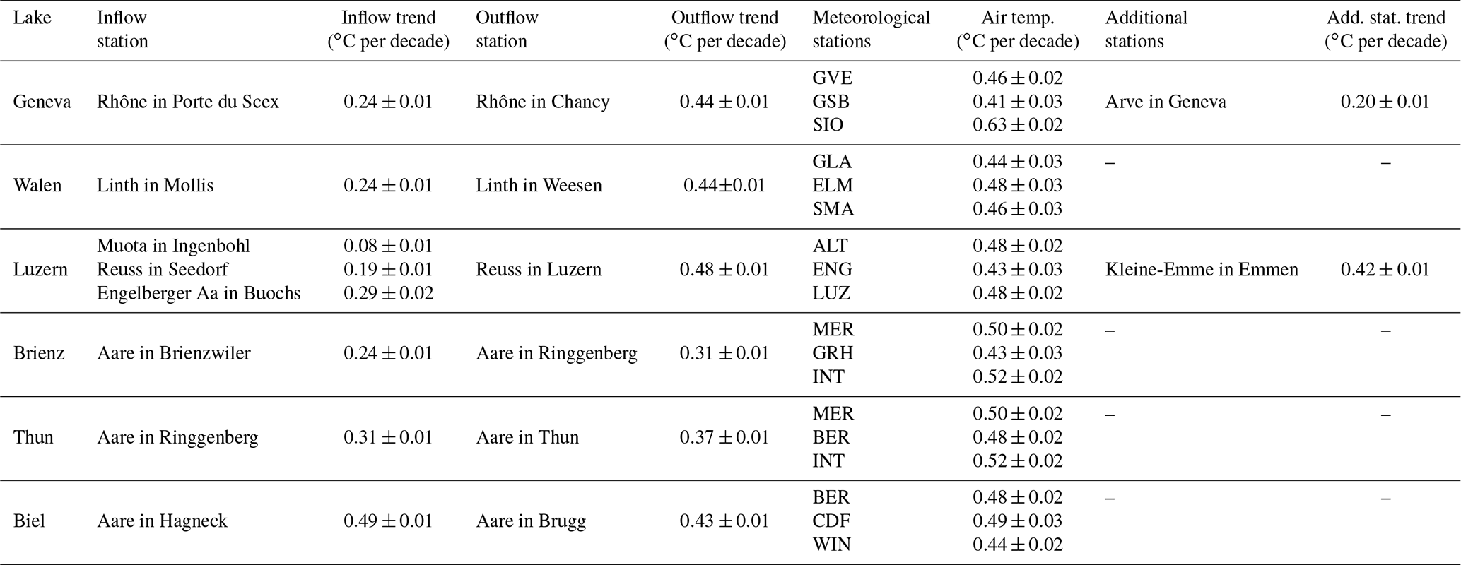
Table 1 Physiographic characteristics and data availability for water temperature and discharge of the 52 selected catchments. The IDs are those used by the data providers, and the IDs followed by an asterisk represent stations where no hourly temperature measurements were available. The providers are the Swiss Federal Office for the Environment (FOEN), the Canton of Bern Office of Water and Waste Management  (AWA), and the Canton of Zurich Office of Waste, Water, Energy and Air (AWEL). For each basin, the selected representative MeteoSwiss meteorological stations are indicated. The details of the abbreviations for the MeteoSwiss stations can be found in Table S2.

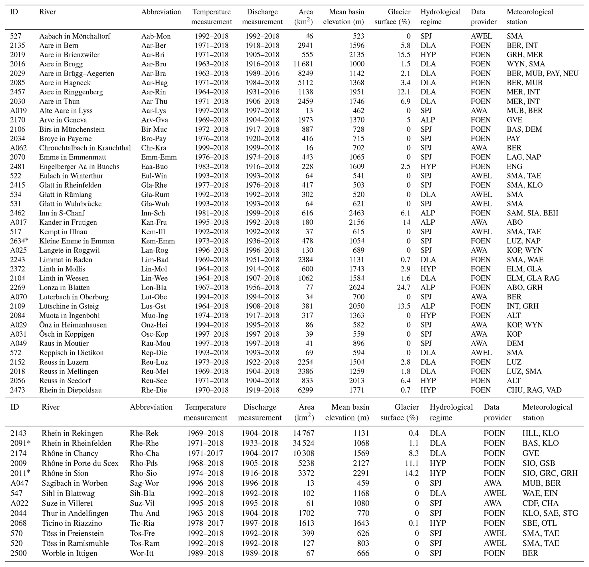
The 52 selected watersheds, presented in Table 1 and Fig. 1, cover a wide range of catchment areas (from a few square kilometres to tens of thousands of square kilometres) and mean elevations (from 450 m to more than 2500 m). Due to the complex topography of the country, the partitioning between solid and liquid precipitation can vary strongly over small distances. Combined with the presence of glaciers in some catchments, this factor naturally influences the hydrological response characterized via the hydrological regime (Aschwanden et al., 1985). The selected catchments are representative of all natural hydrological regimes found in Switzerland except the southern Alps regimes; they can also be influenced by human activities (hydropower production, lake regulation, and water intake or release). The basins are classified into four different categories (Piccolroaz et al., 2016):

• Swiss Plateau/Jura regime (SPJ): in the lower part of the country, most of the precipitation falls as rain. The hydrological response is driven by precipitation and evapotranspiration. The annual cycle with respect to discharge is moderate with a minimum in summer and exhibits high interannual variability depending on regional precipitation patterns.

• Alpine regime (ALP): at higher elevations, both the discharge and thermal regimes are strongly influenced by snow and glacier melt. A pronounced annual cycle is identifiable, with a maximum between March and July depending on the mean basin elevation and on the fraction of glacier coverage, and a minimum during the winter season.

• Downstream lake regime (DLA): Switzerland has many large lakes, and most of them are regulated for flood control purposes (with the notable exception of Lake Constance). As a result, downstream rivers are not only influenced by the lake itself (a natural buffer) but also by its anthropogenic management (extra smoothing).

• Regime strongly influenced by hydro-peaking (HYP): roughly 55 % of Switzerland's electricity production stems from hydropower plants (Schaefli et al., 2019). Storage facilities at high elevation impact the hydrological regime in the lowlands due to controlled intermittent release of large volumes of cold water.

2.2 Meteorological data

One or more meteorological stations, operated by the Federal Office of Meteorology and Climatology (MeteoSwiss), have been associated to each hydrometric gauging station (IDAWEB, 2019). These meteorological stations were selected according to the proximity of the catchments in order to be representative of the local meteorological conditions. Only stations with sufficiently long data records at a daily timescale were kept.

Daily measurements of air temperature and precipitation were compiled, and homogeneous time series (Füllemann et al., 2011) were used whenever available. Homogenization carried out by MeteoSwiss consists of adjusting historic measured values to current measuring standards and locations. Figure 1 shows a map detailing all of the hydrological measurement sites and the associated MeteoSwiss stations. In total, 41 MeteoSwiss stations are associated with one or several catchments. Details on the stations are given in Table S2.

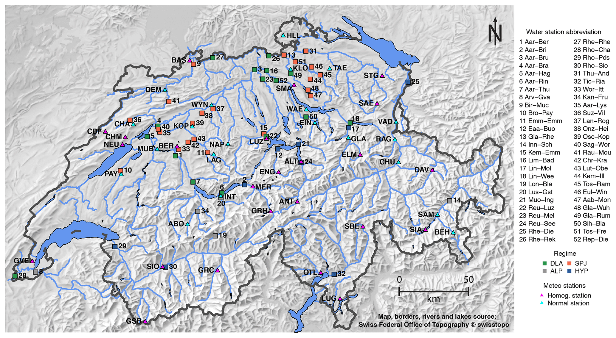
Figure 1 Map of Switzerland showing the selected hydrometric gauging stations and the associated meteorological stations. Abbreviations for hydrometric gauging stations are defined in Table 1, and abbreviations for the meteorological stations are given in Table S2.

2.3 Snow water equivalent and glaciers mass balance

Monthly snow water equivalent maps of Switzerland are used as a proxy for snow melt. These maps are provided by the WSL Institute for Snow and Avalanche Research SLF. They are generated using a temperature-index model in which observational SWE data are assimilated using an ensemble Kalman filter (Magnusson et al., 2014; Griessinger et al., 2016). Glacier annual and seasonal (summer and winter) mean local mass balance and surface extent are available for selected glaciers from the GLAMOS data set (GLAMOS, 2018). The mass balance is estimated based on in situ biannual measurements and then extrapolated to the whole glacier area using distributed modelling and point measurement homogenization techniques (Huss et al., 2015) to retrieve the mean local mass balance. The total mass balance is obtained in this study by multiplying the mean annual and seasonal mass balance (in millimetres water equivalent per year) by the glacier area.

3 Methods

3.1 Data preprocessing procedure

In the analysis below, only complete calendar years are retained; sparse or missing data are allowed as long as gaps do not exceed 2 weeks. For daily averaging, missing data are propagated (i.e. one missing data point during a day results in a missing day), but they are ignored for seasonal and annual averaging. Seasonal and annual time series are used for all interannual comparisons and for inter-variable correlation studies. Daily time series are used for the trend analysis. Indeed, more points are available for daily values than for annual values, leading to more robust trends (see Sect. 3.3).

3.2 Seasonal signal removal

Before applying linear regression to daily data, the seasonal signal is removed using a method called seasonal-trend decomposition based on “loess” (STL) (Cleveland et al., 1990), where loess stands for “locally weighted regression” (Cleveland and Devlin, 1988; Cleveland et al., 1988). This method is robust with respect to outliers in the time series, able to cope with missing data and with any seasonal signal shape, and is computationally efficient. In addition, the seasonality is allowed to change over time and this rate of change is parameterized by the user. The STL method has been widely used in other fields; examples of application in hydrology include the work of Hari et al. (2006), Figura et al. (2011), or Humphrey et al. (2016).

Here, only the main ideas of the method are presented; full details are given in Cleveland et al. (1990). The loess fitting method is a local fitting with weights applied to the points that are fitted. The fitting can be locally linear or locally quadratic, here we use the locally linear fitting following Cleveland et al. (1990). For any x_i in the neighbourhood of x, the loess, or the weight applied to the points before carrying out a local fitting, is defined as follows:

$$\begin{array}{}\text{(1)}& v\left(x\right)=W\left({\displaystyle \frac{\left|x_i-x\right|}{{\mathit{\lambda }}_q\left(x\right)}}\right).\end{array}$$

Note that x_i is the position of the point, not its value. λ_q(x) is defined as the distance to the q_th furthest point, with q being a parameter of the model discussed below. W(x) (Cleveland and Devlin, 1988; Cleveland et al., 1988) is defined by the tricubic function:

$$\begin{array}{}\text{(2)}& W\left(x\right)=\left\{\begin{array}{ll}{\left(\mathrm{1}-x^{\mathrm{3}}\right)}^{\mathrm{3}}& \mathrm{for}\mathrm{0}\mathit{⩽}x<\mathrm{1}\\ \mathrm{0},& \mathrm{otherwise}\end{array}\right..\end{array}$$

Therefore W(x) is large for x_i close to x and becomes zero for x_i further than the q_th farthest point. We can see that q will act as a smoothing parameter on the fit obtained with this method.

In the STL algorithm, vectors of data Y are decomposed as follows:

$$\begin{array}{}\text{(3)}& Y_i=T_i+S_i+R_i,\end{array}$$

where T_i is the trend term, S_i the seasonal term, and R_i the residual term. The algorithm is composed of two iterative loops, called inner and outer loops. In the inner loop, the time series is first de-trended: T_i is extracted and smoothed with a loess fitting as explained above. Then, the seasonal component is extracted using a low-pass filter, and the remaining time series is again smoothed by loess. This process is repeated iteratively and encapsulated in an outer loop. In this second loop, a weight is attributed to each point based on its residual (i.e. $Y_i-T_i-S_i$) such that the weight is low when the residual term is large. These weights are used for the loess fitting in the next round of the inner loop. As the outliers are given a low or zero weight, the method is robust to the presence of outliers. At the end of the loop, R_i is obtained by subtracting the final T_i and S_i from the raw data. Note that the trend term obtained here is a locally fitted function, so it is completely different from the regression parameters obtained by a linear regression, which will later be called the trend.

The STL method has five algorithmic parameters: the number of iterations in the inner loop (n_i), the number of iterations in the outer loop (n_o), the smoothing parameter of the low-pass filter (n_l), the smoothing parameter of the trend component (q), and the seasonal smoothing parameter (n_s). The value of parameter n_l is imposed by the time series sampling frequency and is set here to 365, which is the least odd integer greater than or equal to the time series frequency. The parameters n_i and n_o are set to the recommended values, i.e. n_i=1 and n_o=15 (Cleveland et al., 1990). Following the same recommendation, the parameter q is defined as the first integer respecting the following condition:

$$\begin{array}{}\text{(4)}& q\ge {\displaystyle \frac{\mathrm{1.5}{n}_p}{\mathrm{1}-\mathrm{1.5}{n}_{\mathrm{s}}^{-\mathrm{1}}}},\end{array}$$

where n_p is the time series frequency.

For the seasonal smoothing parameter n_s, no formal recommendation based on previous mathematical analyses exists (Cleveland et al., 1990). This parameter determines the variation of the seasonal signal over time and thus the fraction of the data variation that is included in the seasonal component. If set to a small value, the seasonal component will vary greatly from year to year, including interannual variability. If set to an overly large value, the seasonal component will be exactly the same from year to year, and the method is no longer superior to a simple periodic removal of the seasonal signal (as classically done in hydrological time series analysis, e.g. in Schaefli et al., 2007). The method proposed by Cleveland et al. (1990) to adjust this parameter is not applicable here: it would require an assessment based on 365 different plots per catchment. We propose here to use the autocorrelation function (ACF) and the partial autocorrelation (PACF) of the residuals' time series to select an appropriate n_s. In fact, the ACF and the PACF can be used to ensure that no seasonality remains in the residuals. In particular, the ACF and the PACF of the residuals should not show any significant correlation at the biannual (183 d) or the annual scale (365 d), as this would be indicative of seasonal components being left in the residuals.

Therefore, the following method is applied to all water temperature, discharge, air temperature, and precipitation time series: the STL is run for n_s ranging from 7 to 99 (note that n_s has to be odd and ≥7), and the ACF and PACF are computed for all residuals' time series. The mean ACF and PACF values for lags between 360 and 370 are plotted against the n_s value and the plots are checked individually by visual inspection to determine the best n_s. Visual inspection is justified by the fact that for some catchments and variables, the PACF decreases monotonically and tends to a constant value, whereas in other cases, it reaches a minimum before increasing again, making an automated decision process difficult. Based on this analysis, the value retained for this study is n_s=37, for all variables and all catchments. A single value for all catchments and variables is preferable. Indeed, as this value defines how the signal can evolve over time, and thus influences the trend and the residual terms, different values would make the comparison of linear regression output between catchments and variables less relevant.

Some example outputs of the STL method and additional details are given in Sect. S1.3 of the Supplement. It is noteworthy that the de-seasonalization with the STL method has almost no effect on precipitation. However, in Fig. S4 in the Supplement, we show that the seasonality in precipitation time series is weak.

3.3 Linear regression

The temporal trends are explored using linear regressions over different time periods, which has been shown to be a suitable approach (Lepori et al., 2015) and is commonly used (Hari et al., 2006; Schmid and Köster, 2016). A linear regression is applied to all four de-seasonalized variables (i.e. T_i+R_i from the STL method, for the water temperature, discharge, air temperature, and precipitation variables) against time with the classical least-squares estimation technique. The linear model is applied, when possible, for the 1979–2018 and 1999–2018 periods.

As expected, the correlation determination R² values are relatively low, because the daily and interannual variability is still present in the time series and the linear model cannot represent these components. However, the p values are all very small, and the residuals of the linear model show that, for all periods, the linear regression against time only is a suitable estimator of the trend.

The robustness of the trends is assessed using two independent methods. The first method compares the results from the simple linear model to a robust linear model (Hampel, 1986). This model, which is less sensitive to outliers, is well suited for de-seasonalized temperature time series, but has shown problems with the remaining variability in the de-seasonalized discharge and precipitation time series, including convergence problems for precipitation. For our case study, this method fails to converge for all precipitation time series. The differences in trends obtained by the simple and robust linear models for the four variables are shown in Figs. S9 and S10. The only notable difference is for discharge during the 1999–2018 period.

The second method, which assesses the sensitivity to boundary effects, consists of removing 1 year at the beginning or at the end of the period and recompute the trends (removing 2 years leads to similar results). Figure S11 shows the analysis for the 1999–2018 period. The trends for water and air temperature are indeed lower when the last year (2018, which was extremely warm in Switzerland) is removed, whereas for discharge and precipitation the negative trends are less pronounced when the first year (1999) is removed. These differences are notable, but do not change the main message of the study. For the 1979–2018 period, removing 1 year, both at the beginning or at the end of the time interval, leads to negligible differences, showing the overall robustness of the trends computed over 40 years (see Fig. S12).

The root-mean-square error (RMSE) of the trends obtained over a shorter period is used as a measure of the uncertainty of the mean trend values (the largest RMSEs between trends obtained by removing 1 year at the beginning or at the end are used as the uncertainty value). For single trend uncertainty, the largest difference between the normal linear model trend and trends obtained by removing 1 year at the beginning or at the end is used as the uncertainty value (indicated in Tables A1, A2, S4, and S5).

The linear regressions are also applied to seasonal and annual mean time series. In this case, the R² values are clearly higher, as there is less variance in the input data, but the p values increase. Indeed, only 20 or 40 points are used depending on the time period, reducing the robustness of the method. Some p values are even above the significance threshold. As a consequence, the long-term trends presented in this paper only use de-seasonalized time series, with p values < 0.05. Seasonal trends, obtained from seasonal mean values, must be interpreted cautiously. As a consequence, most of the seasonal analysis is based on raw seasonal means instead of trends due to their low significance level.

For catchments with more than one meteorological station attributed to them, the trends used in the analysis for air temperature and precipitation are the mean of the trends of all the catchment's stations. For precipitation and discharge, they are expressed in relative changes to allow for a comparison between catchments. Unless stated explicitly, trends are expressed per decade.

3.4 Ecological indicators

Two important ecological indicators are used to quantify the impact of river warming and its evolution: the number of days on which stream temperature reaches or exceeds the value of 25 ^∘C, and the number of consecutive days during which the hourly temperature remains above 15 ^∘C.

The 25 ^∘C threshold is a legal limit in Switzerland above which heat release in rivers is forbidden; this is important, for example, for nuclear power plant cooling. The indicator is computed as follows: based on hourly data, when the water temperature reaches 25 ^∘C for at least 1 h, the day is flagged as being above 25 ^∘C. Then, the number of such days per year are summed in order to investigate the evolution over time.

The 15 ^∘C threshold is important for fish health. Indeed, proliferative kidney disease (PKD) affecting salmonid fish is caused by a parasite that proliferates when the water temperature remains above 15 ^∘C for a few weeks (Hari et al., 2006; Carraro et al., 2016, 2017). Thus, water temperature affects the impact of PKD and its prevalence (Carraro et al., 2017).

The indicator is computed following a simple approach inspired by the more complex model proposed in the work of Carraro et al. (2016). First, the days on which the water temperature remains above 15 ^∘C for the whole day are computed (a 3 h moving window average is applied beforehand). Then, data are filtered to keep only series longer than 28 consecutive days. Finally, the number of days above 28 days in the remaining series are summed for each year. The results indicate the number of days in the year for which the temperature was above 15 ^∘C for at least 28 consecutive days. As the process behind PKD is far more complex, this method does not pretend to be exact in determining the presence or absence of PKD in the rivers monitored; however it is an indicative approach to assess the exposure evolution of the river system. A sensitivity analysis has been performed and the qualitative evolution is not dependent on the chosen values for the period length and for the moving average window size.

4 Results and discussion

4.1 Long-term evolution of stream temperature and discharge

The water temperature evolution for all gauging stations used in the current study is shown in Fig. 2a. In spite of the high natural variability, a warming trend is visible in most rivers. To investigate this evolution in detail, catchments with temperature measurements available since 1970 are selected (14 catchments). Figure 2b shows the temperature anomalies per decade with respect to the 1970–2018 mean for these catchments. A two-sided t test is performed to assess if the differences in decadal means are significant. Except between the 1970s and 1980s, where no significant difference is found (p value = 0.17), all of the other respective anomaly means are shown to be significantly different (p values < $\mathrm{5}\times {\mathrm{10}}^{-\mathrm{5}}$ for the three tests) which confirms the important rise observed since 1980 (Fig. 2b). The shift occurring at the end of the 1980s reported by Hari et al. (2006) and discussed in Figura et al. (2011) and Lepori et al. (2015) is not observed in all rivers (see Fig. 2a). Indeed, the shift is clearly visible in catchments located in the Swiss Plateau/Jura regions and downstream lakes, but not necessarily in alpine catchments or catchments strongly influenced by hydro-peaking. Note that this shift is also present in air temperature records (see Fig. S13). The shift between the 1980s and 1990s is more important than previous or subsequent shifts, but contrary to the statement in Hari et al. (2006), the warming trend continues after the shift. Looking at the 30-year anomaly difference, the mean anomaly difference over the 14 catchments for the 1970–2000  period is 0.59 ^∘C and for the 1990–2018 period it is 0.55 ^∘C. A partially overlapping samples two-sided t test (Derrick et al., 2017) finds no significant difference between these two values (p value = 0.59, this test is used instead of a classic t test as the two samples overlap). Consequently, the “end-of-80s” shift might be interpreted as a hiatus in the long-term trend. The apparent acceleration of the warming seen over recent years is due to the extreme year 2018, which pulls up the running mean.

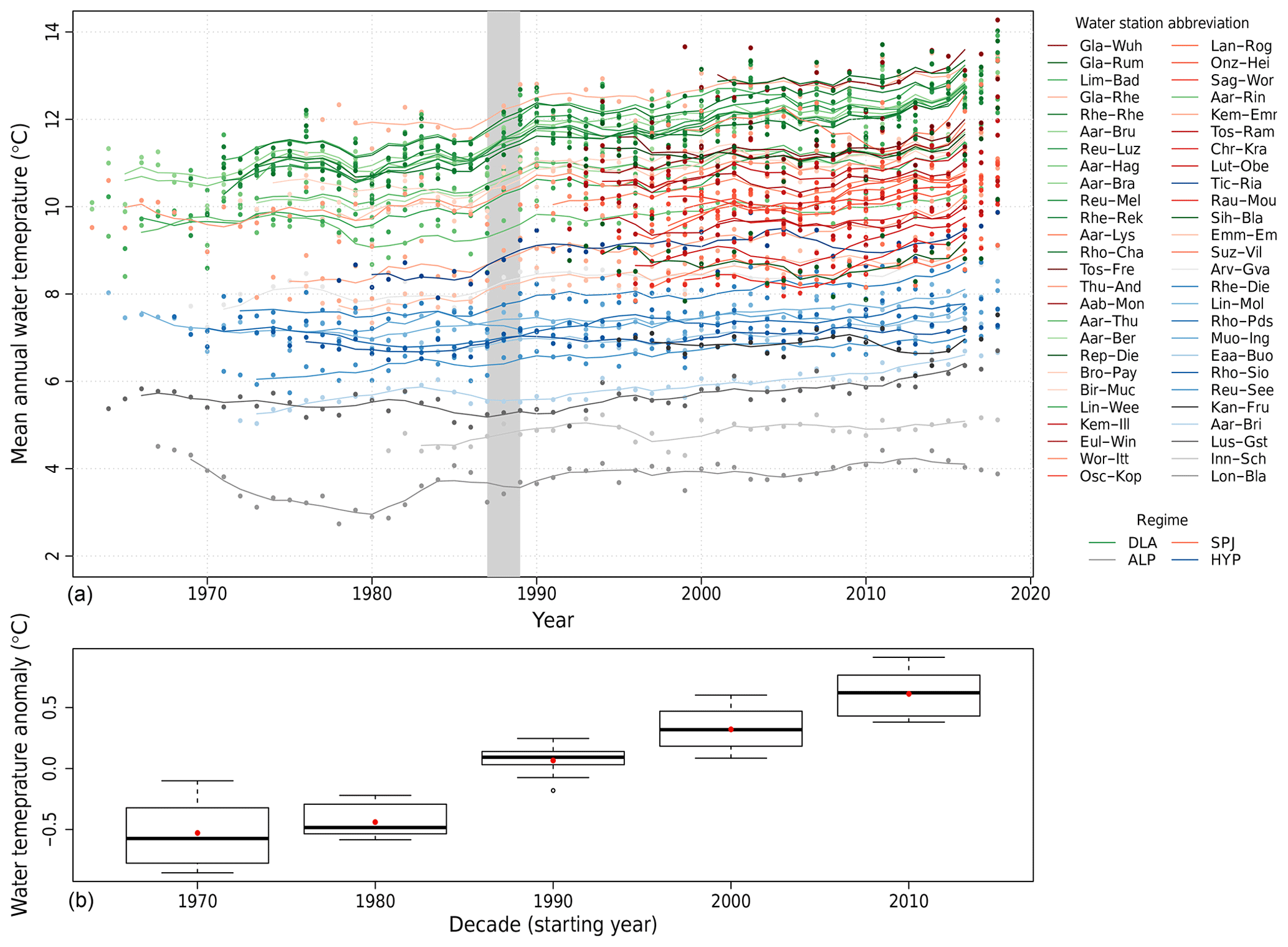
Figure 2 (a) Mean annual stream temperature of the 52 catchments described in Table 1. Lines show the 5-year moving averages. Colours indicate the hydrological regimes. The 1987∕1988 transition period is highlighted using grey. Abbreviation for river names are given in Table 1, and abbreviations for regimes are as follows: DLA represents the downstream lake regime, ALP represents the alpine regime, SPJ represents the Swiss Plateau/Jura regime, and HYP represents the strong influence from hydro-peaking. (b) Water temperature anomalies per decade with respect to the 1970–2018 mean, for the 14 catchments with data available since 1970. Thick lines are the median and red dots the mean values (values used for the t test and the partially overlapping samples t test, see text). Boxes represent the first and third quartiles of the data, whiskers extend to points up to 1.5 times the box range (i.e. up to 1.5 times the distance of the first to third quartiles) and extra outliers are represented as circles.

A long-term analysis is also performed on discharge data (Fig. 3). In this case, catchments with measurements ranging back to at least 1920 (20 catchments) are kept for anomaly analysis. Figure 4 shows that there is almost no trend in the long term for annual mean discharge and precipitation (for the discharge, the mean trend obtained by linear regression over the 26 catchments available between 1970 and 2018 is −0.5 % per decade). However, recent decades have shown a clear negative trend. The 1980s exhibited a positive runoff anomaly with a decrease toward the end of the decade. A 7- to 8-year cycle in the runoff annual mean can be seen in Fig. 3. This is related to the cycle found in the North Atlantic Oscillation (NAO) and the Atlantic Multi-decadal Oscillation (AMO) which has already been discussed in the literature (Lehre Seip et al., 2019). These cycles also have an influence on water temperature as shown by Webb and Nobilis (2007). The time series are presented in Fig. S15.

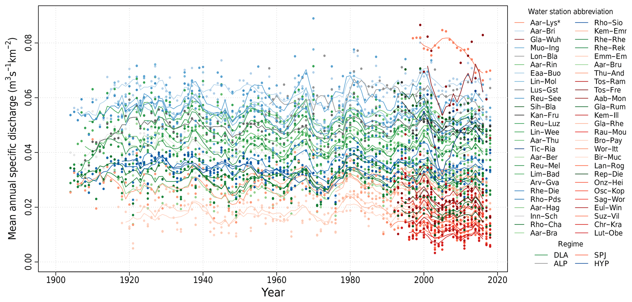
Figure 3 Mean annual specific discharge for the 52 catchments described in Table 1 (normalized by catchment area for comparison). Lines show the 5-year moving averages. Colours indicate the hydrological regimes. Values for the Alte-Aare (Alt-Lys, marked using an asterisk in the legend) are divided by 4 to fit in the plot.

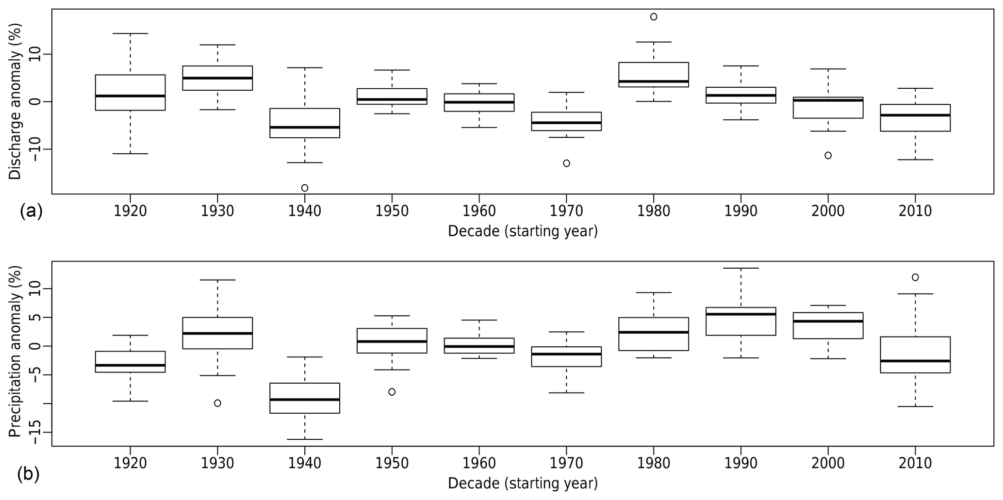
Figure 4 Relative discharge (a) and precipitation (b) decadal means of anomalies with respect to the 1920–2018 average for 20 catchments and 17 MeteoSwiss homogeneous stations with data available since 1920 (see Tables 1 and S2).

A longer multi-decadal variation can be seen in discharge data (see Fig. 4). However, 1 century of data is not long enough to assess if there is a real 30- to 40-year cycle, which could be related to the 34- to 36-year cycle found in the Atlantic Meridional Overturning Circulation (AMOC) (Lehre Seip et al., 2019), or if there is only some statistical variation. As a consequence, it is not possible to assess if the decrease over the last decade is part of a long-term cycle, if it results from climate change, or both.

The decades from 1970 to 1980 and 1980 to 1990 show a more marked anomaly (negative first and then positive, see Fig. 4) for discharge than for precipitation. This is explained by the glacier melt evolution, which reaches a minimum in the decade from 1970 to 1980 followed by a sharp increase in the next decade (Huss et al., 2009).

4.2 Temperature and discharge trends from linear regression

The trends in stream temperature and discharge have been computed using linear regression over the 1999–2018 period for all 52 catchments and over the 1979–2018 period when possible. All trend values are presented in the Appendix in Tables A1 and A2 for water temperature and discharge, and in Tables S4 and S5 for air temperature and precipitation. The plots shown in this section are for the 1999–2018 period, where more catchments are available. Similar plots for the 1979–2018 period are shown in Sect. S2.1. Note that results presented in this section, except for the trends in runoff over the last few decades, also hold for the longer time period, and the results are even more evident over this longer time period. This can be explained by the lower sensitivity to boundary effects and the generally higher robustness of linear regressions over longer time periods.

Trends in stream temperature and discharge are compared to trends in air temperature and precipitation in Fig. 5. There is a clear increase in water temperature and a reduction in discharge observed in Swiss rivers over the 1999–2018 period. The mean trends for the last 20 years are $+\mathrm{0.37}\pm \mathrm{0.11}$ ^∘C per decade for water temperature (with a large spread in the distribution), $+\mathrm{0.39}\pm \mathrm{0.14}$ ^∘C per decade for air temperature, $-\mathrm{10.1}\pm \mathrm{4.6}$ % per decade for discharge, and $-\mathrm{9.3}\pm \mathrm{3.4}$ % per decade for precipitation. However, the trends in precipitation and runoff have to be considered with caution regarding the long-term variation discussed above. For the 1979–2018 period, the mean trends are as follows: $+\mathrm{0.33}\pm \mathrm{0.03}$ ^∘C per decade for water temperature (again with a large spread in the distribution), +0.46 ^∘C ± 0.03 ^∘C per decade for air temperature, $-\mathrm{3.0}\pm \mathrm{0.5}$ % per decade for discharge, and $-\mathrm{1.3}\pm \mathrm{0.5}$ % per decade for precipitation.

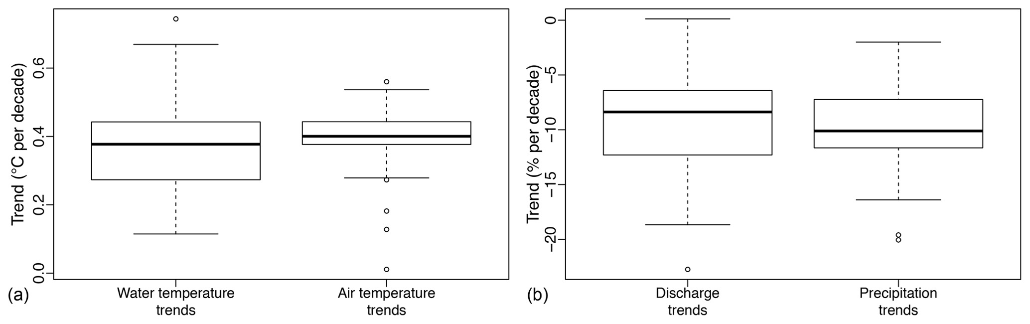
Figure 5 Water and air temperature trends (a) as well as normalized discharge and normalized precipitation trends (b) for the 1999–2018 period and for the 52 catchments described in Table 1 and their associated meteorological stations.

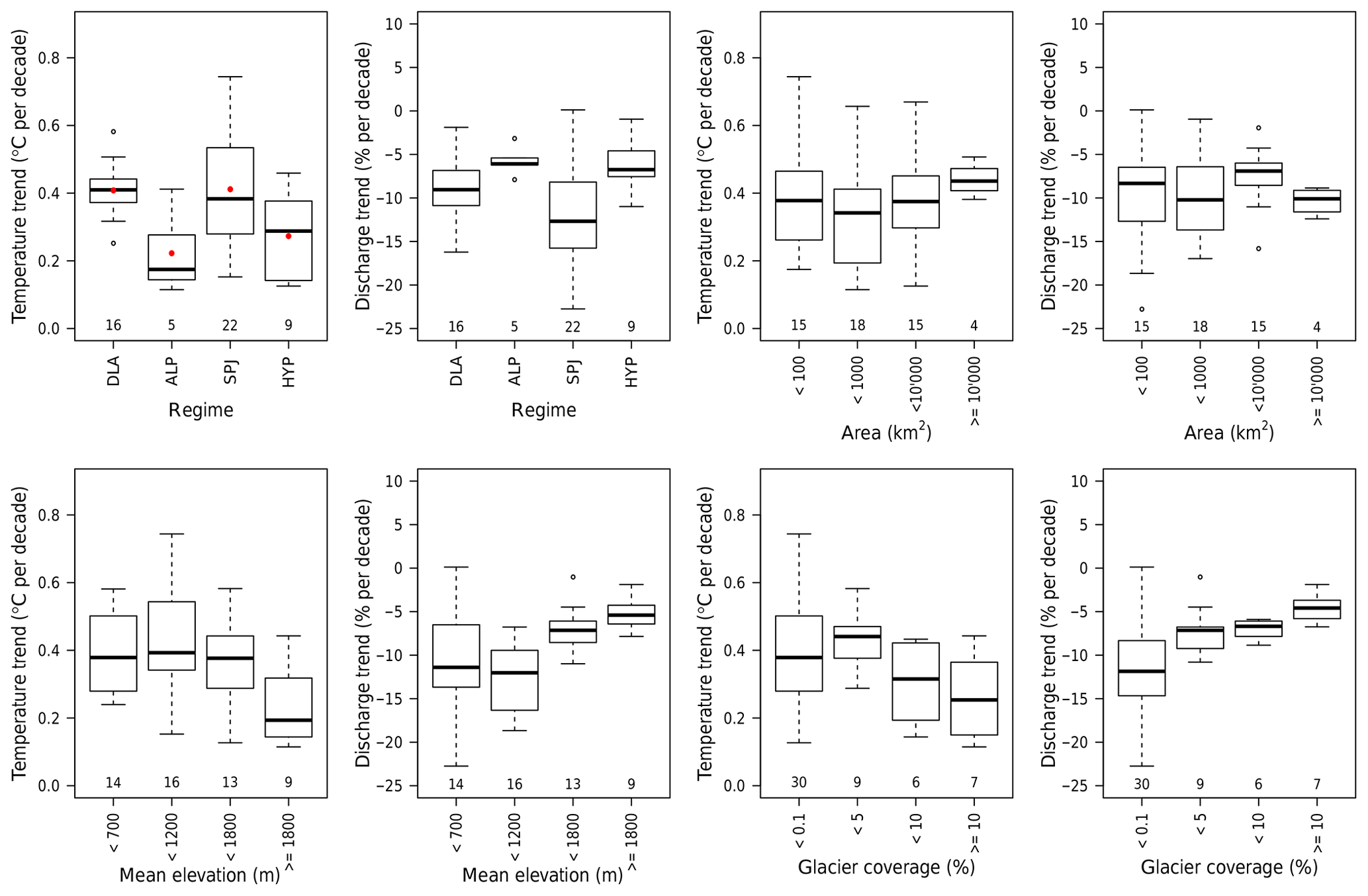
Figure 6 Water temperature and discharge trends for the 1999–2018 period classified by the four different hydrological regimes – downstream lake regime (DLA), alpine regime (ALP), Swiss Plateau/Jura regime (SPJ), and strong influence from hydro-peaking (HYP) (top-left two panels); by the catchment area (top-right two panels); by the catchment mean elevation (bottom-left two panels); and by the glacier coverage (bottom-right two panels). The numbers along the bottom of the panels indicate the number of catchments in each category. In the top-left boxplot, the red dots are the mean values (values used for the Wilcoxon test, see text).

The water temperature and discharge trends for the four different regimes are shown in Fig. 6. Similar plots for air temperature and precipitation are shown in Fig. S14. A two-sided Wilcoxon test is used to assess whether differences between regimes are significant in terms of temperature trends (results shown in Table S3). As some categories only have a few observations and normal distribution can not be assumed, this test is used instead of a t test. Two groups can clearly be identified: the downstream lakes (DLA) regime and the Swiss Plateau/Jura (SPJ) regime on the one hand, and the alpine (ALP) and hydro-peaking-influenced (HYP) regimes on the other hand. Indeed, for both pairs of regimes, the hypothesis of different mean values is clearly rejected with p values > 0.15 (i.e. testing the hypothesis of a different mean between SPJ and DLA and between HYP and ALP). The water temperature trends are significantly lower for alpine catchments and catchments strongly influenced by hydro-peaking. The impact of lakes is discussed in Sect. 4.3.

The catchment area is not correlated with trend values (see Fig. 6) despite the fact that area is clearly correlated with the regime (Table 1). To infer the isolated effect of area, only catchments from the Swiss Plateau/Jura regime are used (largest sample of rivers and no major disturbance), but no correlation between water temperature or discharge trends and area can be found (see Fig. S19).

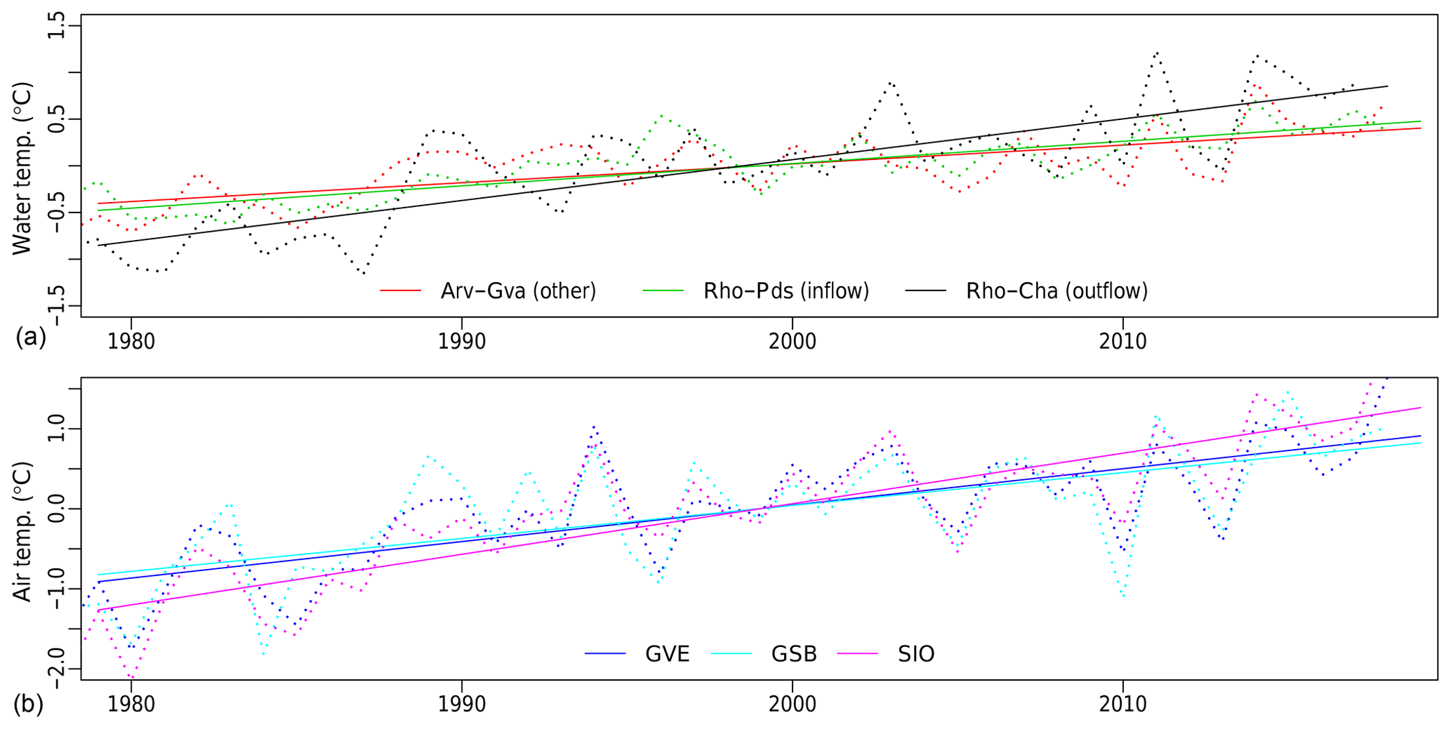
Figure 7 (a) Lake Geneva water temperature anomalies and trends for inflow (Rho-Pds) and outlet (Rho-Cha) stations (a). Arv-GVA denotes the Arve in Geneva, Rho-Pds represents the Rhône in Porte du Scex, and Rho-Cha represents the Rhône in Chancy. (b) Air temperature anomalies and trends for surrounding MeteoSwiss stations. GVE denotes Geneva-Cointrin, GSB denotes Grand Saint-Bernard, and SIO denotes Sion. The period for trend computation is from 1979 to 2018.

Elevation and the fraction of glacier coverage in the catchment (which are strongly correlated) clearly correlate with water temperature and discharge trends (see Fig. 6, bottom row). The smaller positive trends in water temperature and reduced negative trends in discharge observed for highly glaciated catchments can be attributed to cold water coming from glacier melt (as discussed in Williamson et al., 2019), as air temperature trends for alpine catchments are similar to lowland catchments (see Fig. S14). For these reasons, discharge and temperature of alpine streams have been the least impacted by climate change to date. However, if this buffer effect induced by glaciers and seasonal snow cover disappears due to the continuation of temperature rise in the future (Bavay et al., 2013; Huss et al., 2014; MeteoSuisse et al., 2018), the alpine catchments will be amply impacted (see Sect. 4.4.4). Lowland catchments, mostly located in the Swiss Plateau/Jura regions, experience the most important decrease in discharge.

Unsurprisingly, rivers strongly influenced by hydro-peaking show lower temperature trends compared with undisturbed waterways. This results from large volumes of cold water being released from reservoirs located at high elevation to lowland rivers as discussed, for instance, in Feng et al. (2018).

In conclusion, for Swiss Plateau/Jura catchments, air and water temperature trend distributions are similar, and the mean of the trends for this type of catchment is close to the mean air temperature trend (see Figs. 6 and S14). Figures S20 and S21 show water temperature trends for each catchment plotted against trends in air temperature for the 1999–2018 and 1979–2018 periods. Single values (i.e. water and air temperature trends for a given catchment) are poorly correlated. Over the 1979–2018 time period, a better correlation for DLA and SPJ catchments is visible, suggesting that part of the poor correlation in Fig. S20 is due to the noise in the trends obtained with a linear model (boundary effects). For ALP and HYP catchments, the general poor correlation suggests that additional factors, such as snow and glacier melt and anthropogenic disturbances, become predominant in the energy balance, decoupling the mean air temperature and water temperature trends.

4.3 Effect of lakes

In the previous section, it was shown that rivers located downstream of lakes have water temperature trends similar to the Swiss Plateau/Jura catchments, in spite of a higher mean elevation and a larger glacier-covered fraction (see Table 1), which typically attenuate the water temperature increase.

The effect of lakes located at the foot of mountain ranges on stream temperature is well known (Webb and Nobilis, 2007; Råman Vinnå et al., 2018). The input water originates from alpine rivers (potentially disturbed by hydro-peaking), which are colder than the surrounding environment and not in equilibrium with local air temperature. As water has a certain residence time in the lake, its temperature increases due to atmospheric forcing and the main driver for the outflow water temperature is the air temperature. However, it has currently not been demonstrated if the effect of lakes on river temperature trends is similar. In Schmid and Köster (2016), it is shown that lake temperature trends can exceed air temperature trends due to solar brightening.

To investigate the effect of lakes on water temperature trends, five lake systems with measurements at the inflow and the outlet are selected: the Thun–Brienz lake system, Lake Biel, Lake Luzern, Lake Walen, and Lake Geneva. Temperature anomalies with respect to the 1979–2018 period and trends are plotted for water temperature at each station and air temperature at meteorological stations representative of the catchment. The results are shown in Fig. 7 for Lake Geneva and in Figs. S22 to S25 for the other four lakes. The trends for the different inflow and outflow rivers and for air temperature are presented in Table 2.

Table 2 Inflow and outflow water temperature trends for six different lakes, air temperature trends for stations in or close to the lake catchments, and trends for additional catchments mentioned in the text. The period for trend computation is from 1979 to 2018, except for the Engelberger Aa in Buochs where the trend is computed over the 1999–2018 period due to limited data availability.

For Lake Walen and Lake Geneva, the effect is obvious: the outlet trend is almost equal to the co-located air temperature trend. Even if trends in inflows are much smaller, they do not significantly influence the outlet waters (see Table 2). The lake acts as catalyst and the system reaches a quasi-equilibrium. For Lake Geneva, the water temperature of the Arve River is also shown. The Arve River originates from the Mont Blanc massif (France) and flows for about 100 km through the Arve Valley before joining the Rhône in Geneva. Despite flowing through low-lying land, the Arve keeps its alpine characteristics, whereas these characteristics are completely lost in the Rhône River after the lake.

In Lake Luzern, a similar effect is observed. Indeed, the three rivers feeding the lake (the Reuss, Muota, and Engelberger Aa rivers) show trends that are considerably lower than that for the Reuss River in Luzern (see Table 2). However, the Kleine-Emme River, which joins the Reuss just after Luzern, shows a similar trend without the presence of a lake along its course; this demonstrates that, for a mid-elevation stream, flowing a certain distance on the Swiss Plateau leads to a similar effect to that induced by lakes. For the Thun–Brienz lake system, the water temperature trend is enhanced as a result of the two subsequent lakes and it gets closer to the air temperature trend.

For Lake Biel, no effect is observed. This is not surprising as the Aare input water already has a trend similar to the local air temperature. In addition, the residence time in Lake Biel is very short (58 d, whereas for the five other lakes it ranges from 520 to 4160 d; Bouffard and Dami, 2019), limiting the exposure time of lake waters to atmospheric forcing. This has been described in more detail in Råman Vinnå et al. (2017).

In conclusion, despite their higher mean catchment elevation, water temperature trends for stations at lake outlets are similar to Swiss Plateau trends. As lakes have much longer residence times for water than rivers, they smooth out local effects such as snow or glacier melt or precipitation. As a consequence, water temperature trends at the outlet of lakes are generally similar to air temperature trends, which seem to be the main forcing.

4.4 Seasonal trends and relation with air temperature and precipitation

In this section, stream temperature and discharge trends and anomalies are analysed at a seasonal scale. The relation between these two variables and the meteorological conditions (air temperature and precipitation) are also discussed on a seasonal basis. Particular seasonal features are then addressed. Finally, the evolution of the intra-annual variability along with the inter-seasonal correlation, or system memory, are discussed. Even if the inter-variable correlation and system memory are not directly linked to observed changes, they are key factors with respect to understanding the system dynamics and, thus, are essential for inferring the impacts of climate change on water temperature and discharge. The analysis below is mostly based on the 1999–2018 period. Seasons are defined as follows: winter is December–January–February (DJF), spring is March–April–May (MAM), summer is June–July–August (JJA), and autumn is September–October–November (SON).

Long-term evolution of the seasonal anomalies are shown in Figs. 8 and 9 for water temperature (decades from 1970 to 2010) and discharge (decades from 1960 to 2010). Air temperature and precipitation are shown in Figs. S26 and S27 and exhibit similar behaviour. For all seasons, the water temperature has been significantly rising since 1980. The warming is more important in summer and less pronounced in winter. For discharge, spring and autumn do not show an obvious trend in the long term. There is a clear decrease in summer since 1980, whereas winter shows a slight increase.

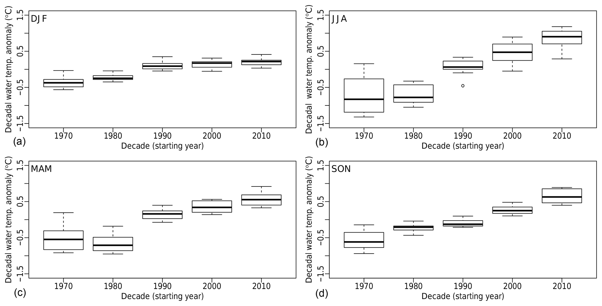
Figure 8 Water temperature seasonal anomalies for the 14 catchments where data are available since 1970 (see Table 1). Anomalies with respect to the 1970–2018 period. Seasons are defined as follows: winter is December–January–February (DJF, a), spring is March–April–May (MAM, b), summer is June–July–August (JJA, c), and autumn is September–October–November (SON, d).

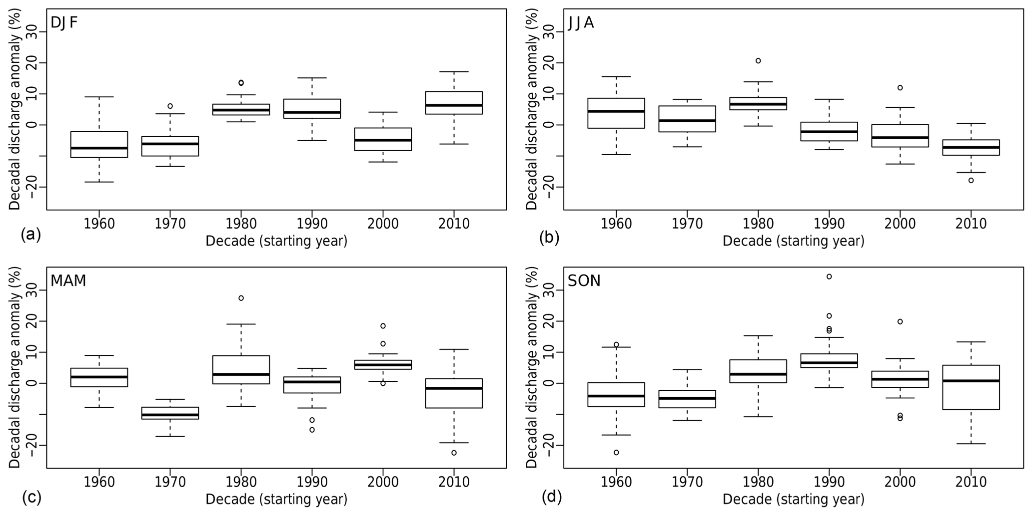
Figure 9 Discharge seasonal relative anomalies for the 26 catchments where data are available since 1960 (see Table 1). Anomalies with respect to the 1960–2018 period.

Annual and seasonal trends for stream and air temperature, discharge, and precipitation are presented in Fig. 10 for the 1999–2018 period. They confirm the tendencies described above. Mean water temperature trends are slightly smaller than air temperature trends for all seasons except for spring, when they are notably larger. This shows that rivers do not react linearly to a general warming of the atmosphere and additional factors control these complex systems. For discharge, negative trends are found in all seasons except for winter, when they are almost zero. Discharge trends follow precipitation trends in all seasons. In general, precipitation determines the discharge trend; consequently, snow and glacier melt play a minor role in the observed trends. However, for specific catchments, this can be different. When looking at individual catchments, there is only a insignificant correlation between trends in air and water temperature, and between trends in discharge and precipitation (see Table S6). This absence of a correlation results from the noise in the individual trend values due to the short time period available. This is a limitation of the method applied and, thus, trends can not be used for an inter-variable interaction study.

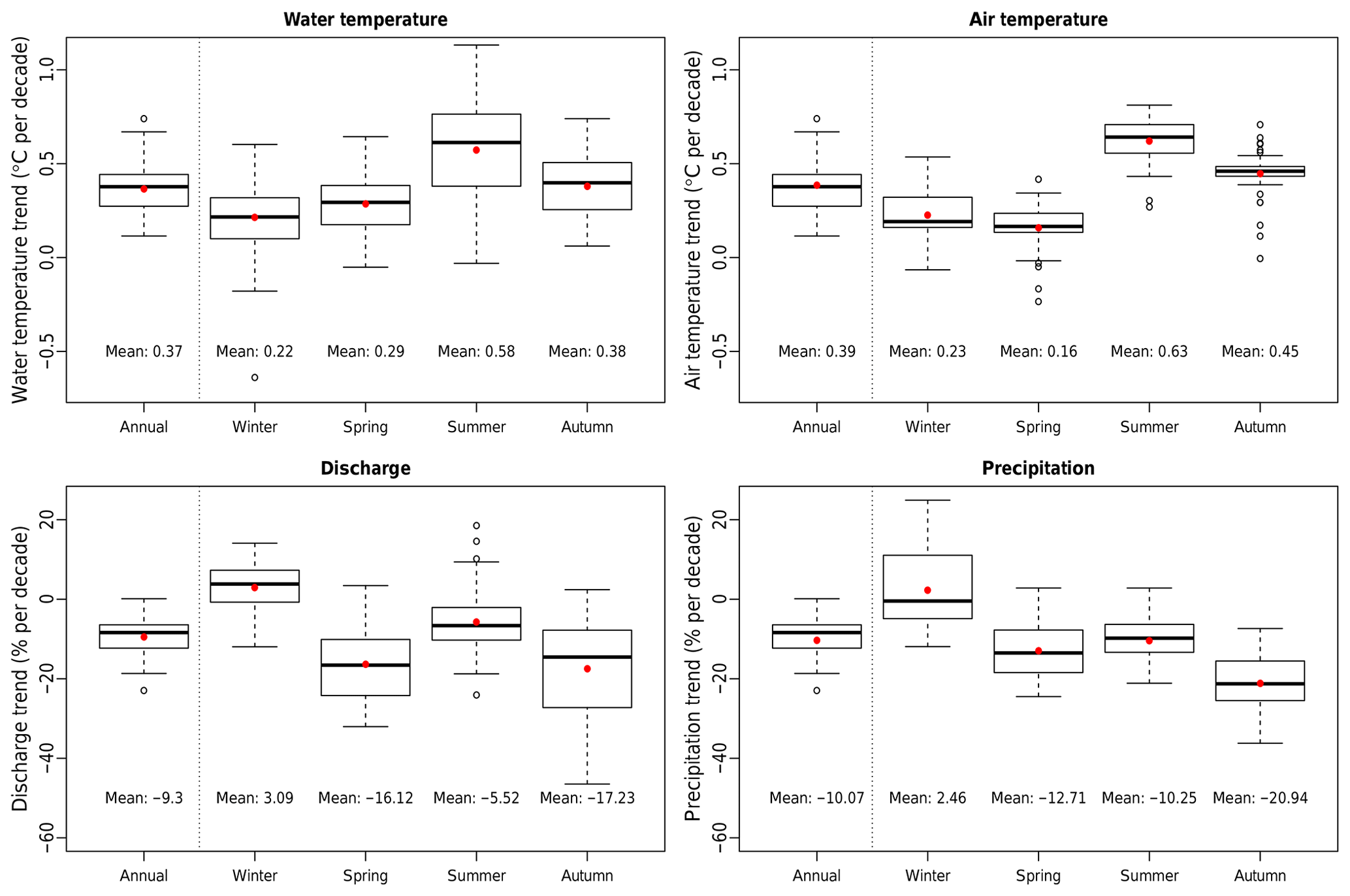
Figure 10 Annual and seasonal trends for water temperature, air temperature, discharge, and precipitation for the 1999–2018 period. The mean values are indicated by red dots and written below the boxes in degrees Celsius per decade or percent per decade.

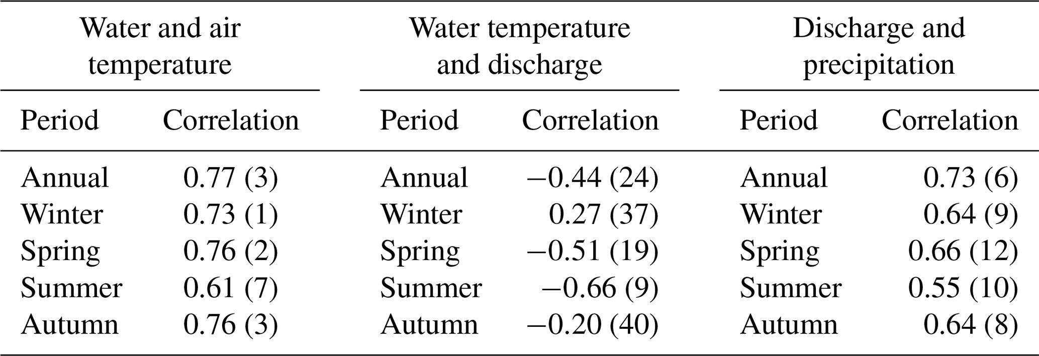
To explore the correlation between variables, raw values are used. Table 3 shows the correlation between main variables on a yearly and seasonal basis. These values are obtained by computing the correlation of two variables for individual catchments and then averaging these correlations. As a measure of the robustness of the method, the number of catchments where correlations are insignificant (p value > 0.05) is indicated. At an annual scale, air temperature is the main driver of water temperature. The negative correlation between water temperature and discharge is rather weak and is not significant in almost half of the catchments. As expected, discharge and precipitation are strongly correlated.

Table 3 Correlation between the annual and seasonal time series of water and air temperature (left), water temperature and discharge (middle), and discharge and precipitation (right). Correlations are computed for all 52 individual catchments over the 1999–2018 period and then averaged over all catchments. Numbers in parentheses indicate the number of catchments where the correlation is not significant (p value > 0.05, with the null hypothesis being no correlation).

4.4.1 Winter

The water temperature trends in winter are the lowest of the four seasons and the discharge exhibits a slight positive trend, as opposed to the negative discharge trend in all other seasons (see Fig. 10). The positive trend in winter discharge is mainly driven by the increase in winter precipitation. This is the season where the precipitation and discharge trends are the closest, and the correlation between precipitation and discharge is strong and significant (see Table 3).

There is a weak positive correlation between winter discharge and winter water temperature. Even though this correlation is not significant in the majority of the catchments, it indicates a different behaviour compared with spring and summer. An explanation for this could be that increased water input during winter causes a push of relatively warm groundwater. Thus, catchments with increased winter discharge would have a more pronounced temperature trend. In contrast, some catchments show negative water temperature and discharge trends in winter (see Appendix Table A1). In this case, the lower discharge favours a more pronounced water cooling via heat exchange, and this effect might compensate for and even overcome the air temperature trend. Both of these effects would lead to a positive correlation. The annual anomalies in winter water and air temperature, discharge, and precipitation are presented in Fig. S28.

4.4.2 Spring

In spring water temperature trends are more pronounced than air temperature trends (see Fig. 10). Looking at individual catchments indicates that those most affected are mainly low-lying, non-glacierized SPJ catchments (see Appendix Table A1). These catchments experience the most significant discharge decrease in spring, probably due to an earlier snow melt period, which possibly explains their higher sensitivity to air temperature. Indeed, snow melt releases cold water that acts as a buffer and reduces the sensitivity to air temperature (Williamson et al., 2019). Figure S29 shows the yearly anomalies in spring. The air temperature remains the main driver; however, high discharge (e.g. 1999 or 2006) or low discharge (e.g. comparing 2013 and 2015) conditions also have a clear anti-correlated impact on water temperature. This can be seen in the negative correlation between air temperature and discharge in spring (Table 3).

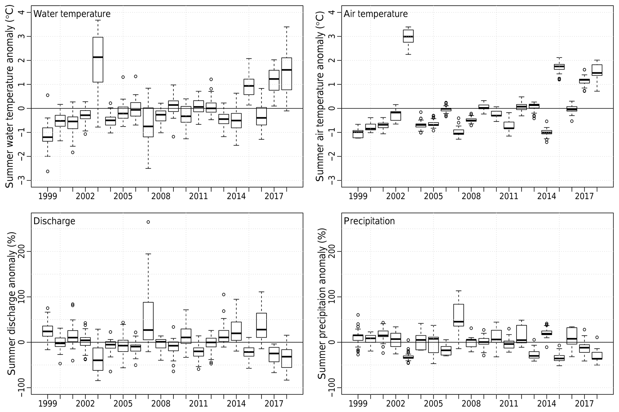
Figure 11 Summer anomalies in water temperature, air temperature, relative discharge, and relative precipitation for all 52 catchments. Anomalies are computed with respect to the 1999–2018 mean for each catchment.

A likely impact of climate change is an earlier and shorter snow melt season. Figure S32 shows the evolution of snow melt in terms of snow water equivalent (SWE) in spring over the last 20 years for Switzerland. There is no clear long-term trend in the total spring melt and, therefore, no contribution to the discharge trend on a seasonal basis (this does not exclude a shift in runoff timing due to earlier snow melt in spring). However, snow melt remains a key factor for spring discharge. For example, in 1999, 2009, 2012, and 2018, precipitation deficits are well compensated for by the above-average snow melt, whereas in 2002 and 2007, the opposite effect is observed. Such discharge variations have a direct impact on water temperature.

4.4.3 Summer, extremes, and autumn

Summer exhibits the strongest positive water temperature trends and negative discharge trends, both in the past 20 and 40 years (see Fig. 10 and Appendix Tables A1 and A2). It also has the weakest correlation between water and air temperature and the strongest negative correlation between water temperature and discharge (see Table 3), suggesting that summer is the season when water temperature is the most sensitive to discharge. Moreover, correlation between precipitation and runoff is lowest in summer. This is likely due to the role of evapotranspiration in summer and the variability of the remaining snow at the beginning of summer (see Fig. S31). There is a strong link between extremes in summer air temperature (2003, 2015, and 2018) and extreme summer stream temperature (see Fig. 11), coinciding with a deficit in precipitation and in discharge. A positive air temperature anomaly in summer is generally associated with dry conditions in Switzerland (Fischer et al., 2007a, b). Sometimes, a below-average air temperature but an above-average water temperature is observed, e.g. in summer 2011. This is attributed to the lack of precipitation and the resulting runoff deficit. Therefore, while precipitation deficit favours and enhances summer heat waves, it also has a direct impact on the summer stream temperature. The years 2013 and 2016 show a negative water temperature anomaly, whereas the air temperature is close to the mean. This is likely due to the above-average precipitation and runoff for these years. Therefore, the water temperature to discharge and precipitation negative correlation holds for both high and low values.

Summer snow melt, approximated by the amount of snow remaining at the beginning of June, shown in Fig. S21, has an impact on summer stream conditions. Indeed, for high summer snow melt, (e.g. 1999 and 2013) the runoff anomaly is positive and stronger than the precipitation anomaly. The opposite effect is seen in 2005 or 2011: the snow melt is low in summer, with a direct impact on stream temperature.

The anomalies in autumn are presented in Fig. S30. Discharge has a very low impact during this season. As air temperature is the main driver, the interannual variability in autumn is lower for water temperature than for air temperature.

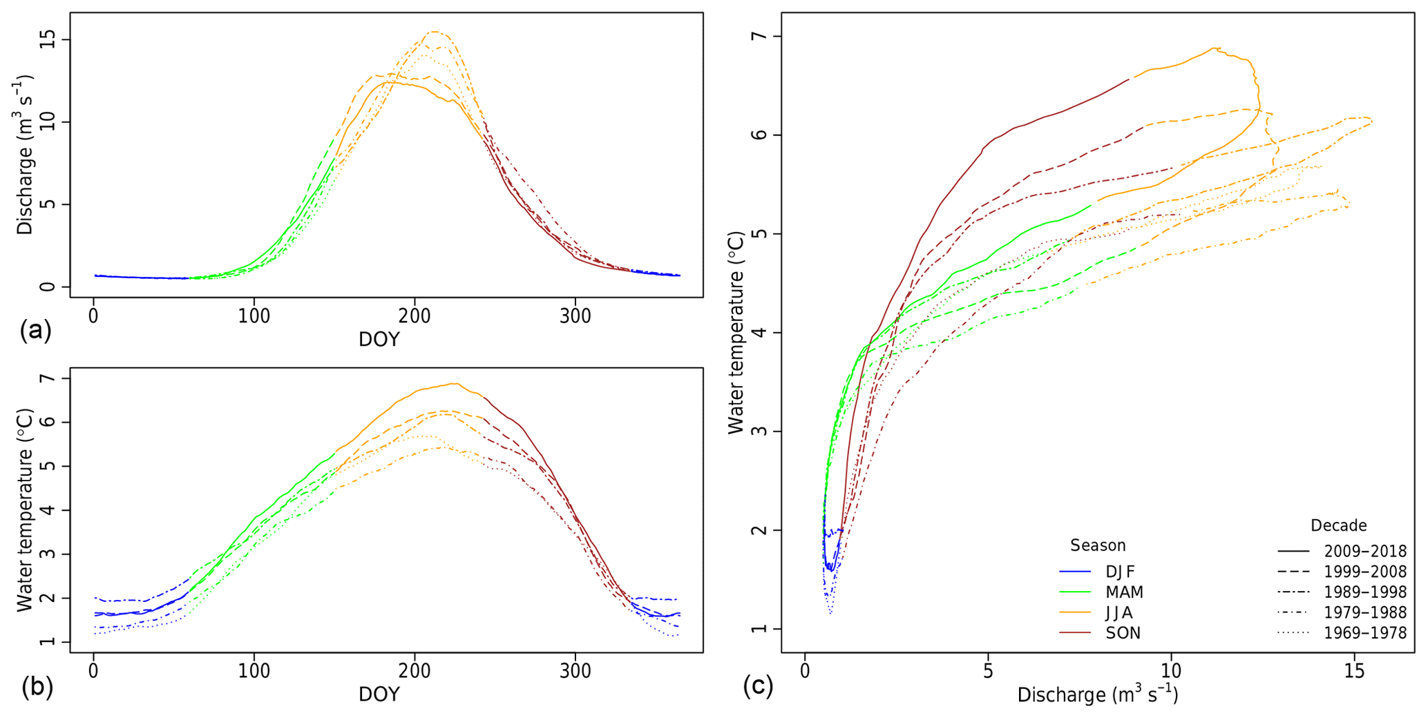
Figure 12 Hydrological (a) and thermal (b) regimes per decade for the Lonza River in Blatten averaged for each day of the year (DOY). Line types represent decades and colours denote the seasons. (c) Decadal temperature plotted against decadal discharge (both averaged for each day of the year).

4.4.4 The case of alpine catchments

The analysis in the previous sections did not considered the hydrological regime. However, alpine catchments show a particular behaviour. Over the last 2 decades, higher-elevation catchments have exhibited lower stream temperature trends and less pronounced discharge decreases than lowland rivers (see Fig. 6 and S18). In addition, water temperature trends are notably less important than air temperature trends. Similar behaviour has also been observed in North America (Isaak et al., 2016). In winter, the air temperature trend is higher in the mountains than for the rest of the country, while the water temperature trend is smaller, showing the impact of enhanced snow melt induced by higher air temperatures, and thus cold water advection in rivers, as discussed in Sect. 4.4.1. The same effect is seen in spring. In summer, the temperature trend is mainly driven by the local air temperature trend, which is lower than the median of the whole country, leading to a lower warming in alpine rivers than in lowland waterways (see the top two rows of Fig. S35).

Alpine catchments are more preserved from extreme summer temperatures than other catchments (see years 2003, 2015, 2017, and 2018 in Fig. S35, bottom two rows). Despite an important positive anomaly in air temperature, the water temperature anomaly is considerably lower and below the median of catchments of other regimes. This resilience is attributed to many factors impacting alpine river temperatures such as geology, topography, or permafrost (Küry et al., 2017) and, in the case of the extreme 2003 heat wave, additional cold water released from glacier and snow melt during summer (Piccolroaz et al., 2018). This is confirmed by the positive or weakly negative runoff anomaly over this year for alpine catchments, whereas the Swiss median anomaly in discharge is negative and the precipitation anomaly is clearly negative too (see Fig. S35, bottom two rows). In addition, a peak in glacier melting in 2003 is visible in the glacier mass balance of the GLAMOS (Glacier Monitoring Switzerland) records (see Fig. S33).

While this low sensitivity is obvious for 2003, when alpine catchments were almost not affected, the sensitivity seems more pronounced in 2015, 2017, and 2018. For these 3 years, the water contribution from glacier melt is lower, as shown by the mass balance glacier record (see Fig. S33) and by the fact that discharge anomalies for these years are closer to the mean of all catchments. Some catchments, e.g. the Lütschine in Gsteig, indicate that the way alpine streams react to summer air temperature and heat waves seems to change. This change is most probably induced by climate change. Note however, that the way alpine rivers respond to heat waves is a recent and not fully explored topic (Piccolroaz et al., 2018).

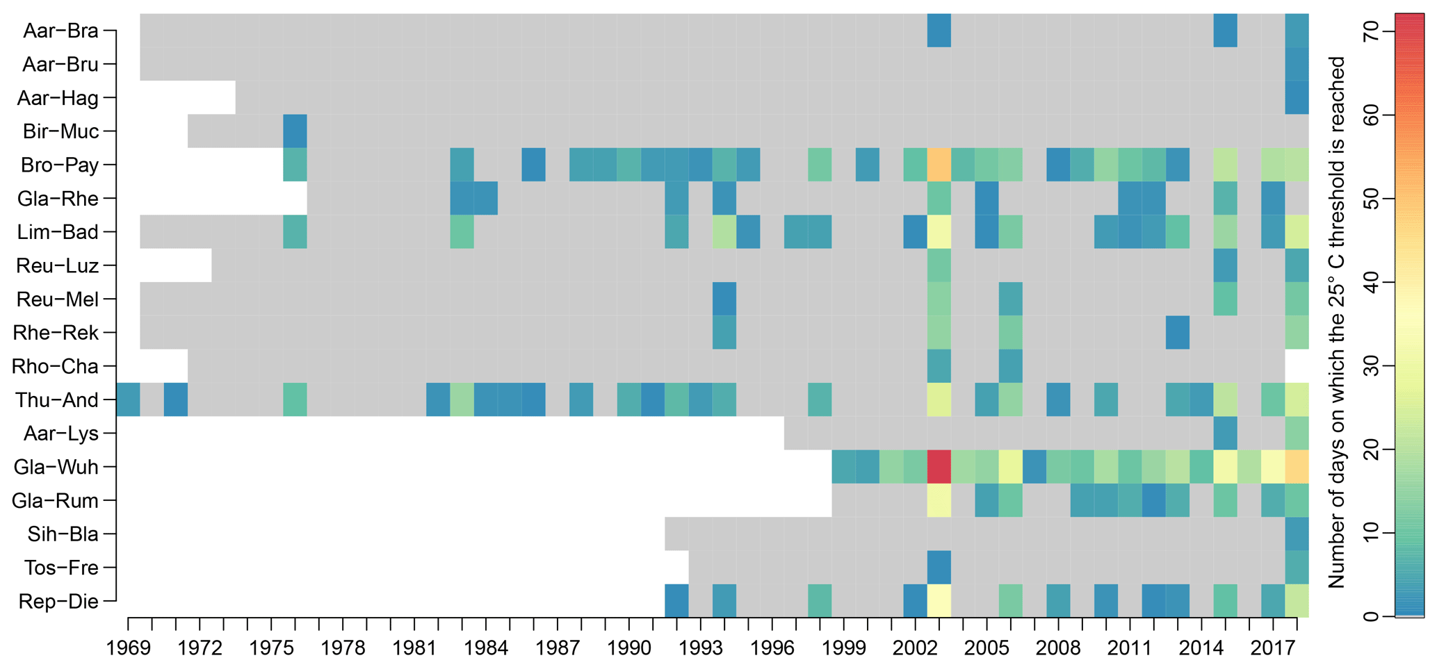
Figure 13 Number of days per year when the 25 ^∘C threshold is reached (i.e. water temperature is above 25 ^∘C for at least 1 h during the specific day). Only catchments where the threshold is reached at least once are shown. Abbreviations of catchments names are explained in Table 1.

In the long term, a shift of the thermal and hydrological regimes of alpine catchments is evident. For example, Fig. 12, obtained by averaging each day of the year (DOY) over an entire decade, shows a clear flattening of the discharge curve over the last 50 years for the Lonza River (glacier surface: 24.7 %). Instead of a peak in the second half of the summer, the last 2 decades show a flatter discharge with a maximum at the end of June. In addition, the entire discharge distribution is shifted towards the beginning of the year, leading to an increase in spring and a decrease in late summer and autumn. There is a clear increase in water temperature, especially between mid-spring and mid-autumn, which is stronger in the middle of the summer, leading to a wider temperature range throughout the summer. This shift in hydrological regime and general warming significantly changes the evolution of the water temperature versus discharge hysteresis curve. While in the 1970s, the amplitude of hysteresis was rather limited (i.e. low sensitivity to summer air temperature), it becomes much wider over the last few decades as a result of lower peak discharge and a higher water temperature. This is an additional evidence that alpine rivers are becoming more sensitive to climate change, and will potentially react in a strongly non-linear way in the future. Similar plots for the Arve in Geneva and the Lütschine in Gsteig are shown in Figs. S36 and S37, respectively (time series from the last two alpine catchments are too short to produce such plots).

4.4.5 Intra-annual water temperature variability, inter-seasonal correlation, and system memory

With the summer water temperature trend being stronger than the winter trend, the intra-annual variability, i.e. the summer to winter temperature difference, is expected to increase over time. The topic of the variability of air temperature under climate change is still an open discussion (Vincze et al., 2017). Figure S34 shows the annual difference between summer and winter means for all catchments with data since at least 1980. There is a clear evolution of the intra-annual variability: the computed trend indicates an increase of 0.3±0.1 ^∘C per decade, which corresponds to a change of +1.2 ^∘C over the studied period and represents an increase of 10 % to 20 % of the variability for individual catchments. The evolution of the summer to winter difference induced by the different seasonal warming rates is thus not negligible and must be considered when assessing the impact of climate change on ecosystems, which will have to cope with warmer conditions but also with an increased variability.

It is well known that the 2003 summer heat wave in Europe was enhanced by a long dry spell due to a precipitation deficit in late spring and early summer (Fischer et al., 2007b). The current data set allows for the assessment of whether such robust seasonal connections exist with stream temperature and discharge. The seasonal relation can be studied by comparing Figs. 11, S28, S29, and S30. In addition, the correlations between water temperature and water temperature from previous seasons, between discharge and precipitation from previous seasons, and between water temperature and precipitation from previous seasons are shown in Table S7. For water temperature, there is almost no correlation and calculated values are mostly not significant. There is also no strong correlation between precipitation and discharge more than one season apart. The correlation with the next season is weak and only significant for a few catchments, showing that the groundwater storage plays an important buffer role (see Sect. S2.3 for an extended discussion).

Despite this lack of strong correlations in the long term, connections exist for some individual years. A negative relation between spring discharge and summer temperature exists (e.g. 2003 and 2017; see Fig. 11 and S29). However, 2004, 2005, and 2011 have an important precipitation deficit in spring, without any noticeable above-average water temperature in summer, meaning that a spring precipitation deficit can contribute to a positive summer stream temperature anomaly, but the summer conditions (air temperature and precipitation) remain the main controlling factors and can cancel the spring effect. In autumn, impacts of extreme summers such as 2003 or 2018 are no longer noticeable in the mean stream temperature (see Figs. 11 and S30). In summary, no strong memory patterns could be identified in the hydrological system. While it might be important for more complex systems (e.g. the land–atmosphere interaction), the antecedent state of the system is not really relevant for the catchments studied.

4.5 Ecological indicators

In this section, two ecological indicators based on water temperature are presented. The first one is the number of days per year when the stream temperature exceeds 25 ^∘C for at least 1 h during the day. Rivers reaching this threshold at least once in the past are shown in Fig. 13. The summer discharge anomaly for these catchments is shown in Fig. S38.

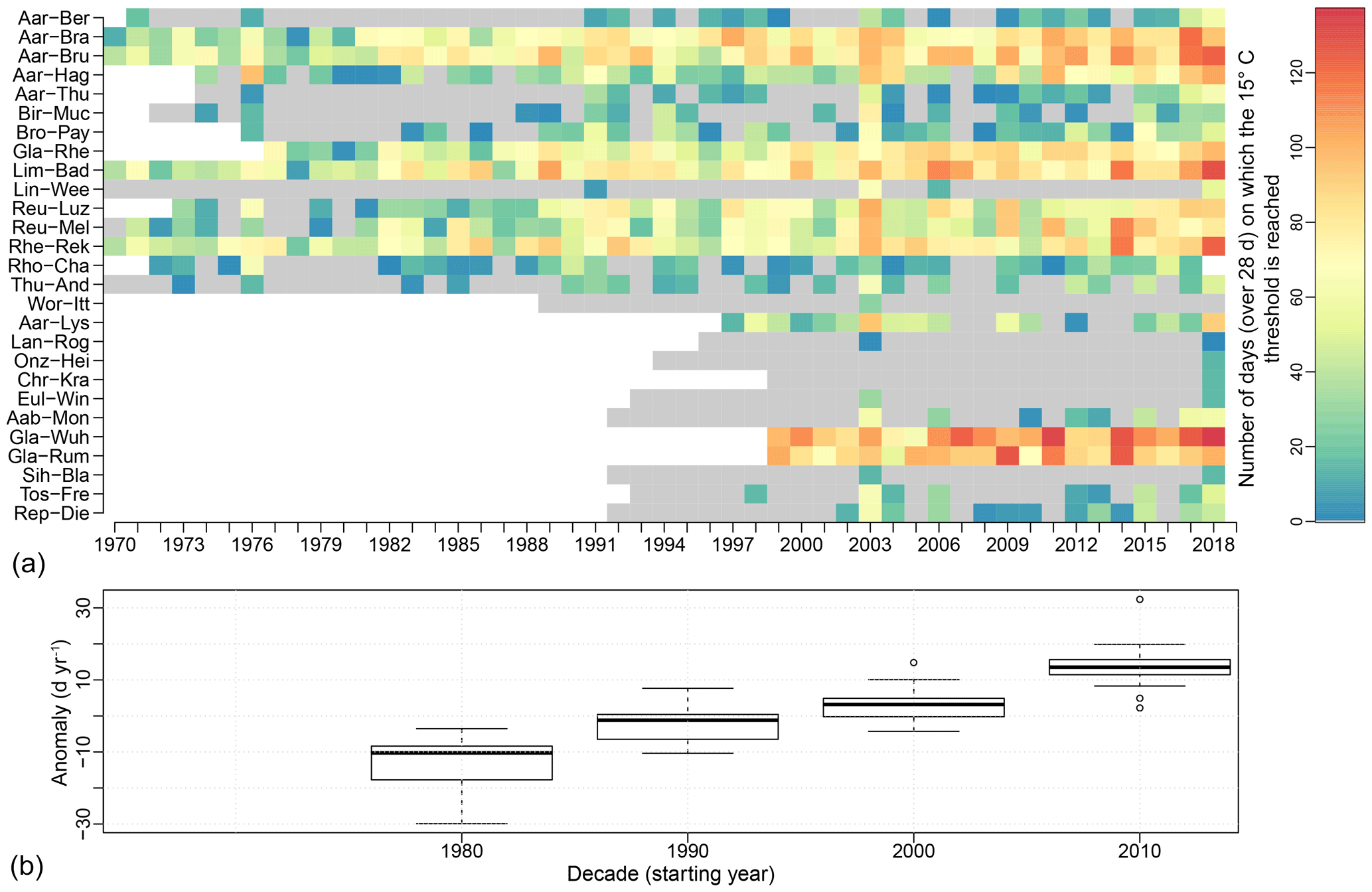
Figure 14 (a) Number of days per year when the water temperature was above 15 ^∘C for at least 28 d (first 28 d not counted). Abbreviations of catchment names are explained in Table 1. (b) Anomaly in the decadal mean number of annual days when the water temperature is above 15 ^∘C for at least 28 d (first 28 d not counted) for the 15 catchments where data are available since 1980. Anomaly with respect to the full period mean.

There is a noticeable increase in warm water events over the few last decades. The extreme years of 2003 and 2018 are clearly highlighted. The occurrence of warm days is often related to discharge deficit, i.e. low flow conditions. However, while peaks above 25 ^∘C were only occurring along with a discharge reduction in the 1970s and 1980s, this is no longer the case in the last few decades (see e.g. years 1994, 2007, and 2012), indicating that the Swiss river system is becoming more sensitive and more exposed to these extreme temperature events with ongoing climate change.

The second threshold is the consecutive number of days above 28 d for which the temperature constantly remains above 15 ^∘C, which is critical with respect to the spread of the proliferative kidney disease (PKD). Figure 14 shows the number of days per year during which fish would be exposed to PKD. There is a clear increase over the past few decades (see Fig. 14b), and some rivers that were almost preserved before 1990, such as the Aare in Bern (Aar-Ber) or the Broye in Payerne (Bro-Pay) have become increasingly affected over the last 2 decades. During extremes years, such as 2003 and 2018, the increase is particularly visible.

Most of the measurement sites where such warm water events were observed are located downstream of lakes and in relatively large catchments, or at low elevation on the Swiss Plateau (e.g. the Broye or the Glatt rivers). Some catchments at higher elevation are also affected (e.g. the Linth in Weesen – Lin-Wee, which has a mean basin elevation of 1584 m). Looking at the temporal distribution of days above the 15 ^∘C threshold (not shown), they mostly occur between June and mid-October. Over time, there is a clear shift to earlier occurrences in the year, although the temporal conclusion of these events remains constant.

5 Conclusions and outlook

This detailed analysis of stream temperature and discharge trends in Switzerland, along with relevant meteorological variables, found strong evidence that climate warming over the last few decades has had a clear influence on the stream temperature in this largely alpine country. Specifically, it is shown that stream temperatures have continued to rise after the shift observed in 1987/1988. For the 1979–2018 period, the mean warming rate is +0.33 ^∘C per decade (for the available 31 catchments), and for the 1999-2018  period, the mean warming rate is +0.37 ^∘C per decade (considering 52 catchments). This later rate corresponds to about 95 % of the contemporary air temperature warming rate. Similar mean trends have been observed in Germany, Wales, and England over comparable periods (Orr et al., 2015; Arora et al., 2016). At the individual catchment scale, air and water temperature trends are poorly correlated, suggesting the large influence of local conditions and hydrological processes on water temperature. The warming is more pronounced in summer and less important in winter, creating a gradually increasing winter to summer stream temperature difference, which is in agreement with results found by Moatar and Gailhard (2006), Webb and Nobilis (2007), and Arora et al. (2016) in France, Austria, and Germany, respectively, but differs from the observations in Wales and England (Orr et al., 2015), that can be easily explained by the different climate conditions over Great Britain. In spring, the water temperature trend is more pronounced than the air temperature trend (consistent with Huntington et al., 2003 and Webb and Nobilis, 2007). While in general the warming of streams is mainly driven by the air temperature, we show that discharge conditions and snow or glacier melt also play an important role, especially in summer. Furthermore, our analysis clearly reveals the role of snow melt in creating resilience to warming in high alpine streams (as found in North America in Isaak et al. (2016)). However, this resilience is likely to decline in the near future due to expected further decreases in snow cover. We also show that the presence of lakes speeds up the shift from limited trends in alpine streams to larger trends on the Swiss Plateau (as found in Webb and Nobilis, 2007), whereas the catchment area does not have a strong statistical correlation with the observed water temperature trend.

The impact of past climate change on discharge, a key driver of stream temperature, is less clear. A decrease of 10 % per decade is observed over the 1999–2018 period. This decrease is more evident in spring and autumn, whereas a small increase is observed in winter. The annual discharge evolution is closely related to the annual precipitation evolution. In the longer term, there are some oscillations in the observed discharge and precipitation time series, and mean discharge similar to today's values were already observed in the past. Therefore, it is not currently possible to assess whether there is a tangible impact from climate change on discharge at the country scale in Switzerland.

The relevance of the identified trends for water resource and ecosystem management is underlined by the analysis of temperature threshold exceedance during summer. We show that the legal limit for stream temperature in Switzerland (25 ^∘C), beyond which heat release in any form is prohibited, has been reached more often during the past few years and that the conditions for the development of proliferative kidney disease in fish have also been met more frequently than in the past. Considering the expected continuation of air temperature rise in Switzerland (MeteoSuisse et al., 2018), our study shows the urgent need for adaptation and mitigation strategies to preserve the fluvial ecosystems of Switzerland and mitigate the impacts on the Swiss economy and energy production sectors.

While it was attempted to cover and investigate the main hydrological regimes of Switzerland in this study, only five stations for alpine catchments and one station for the southern Alps (Ticino) region had long enough time series for analyses. This is owing to the fact that water temperature is a recent serious concern, and the stream temperature measurement networks in the Swiss cantons have mainly been installed since 2000. Based on the present denser network for stream temperature monitoring, and in view of the expected continuation of temperature rise, it would be interesting to repeat a similar study with the additional available stations some years from now in order to detect changes and new trends.

Besides the trend analysis, a key objective of this study was to investigate physical mechanisms underlying stream temperature in different hydrological regimes. The results show that there is no strong memory effect on the system with respect to stream temperature. The water temperature, stream discharge, and the meteorological conditions generally have a weak impact on the next season. The strongest effect observed is the impact of a warm and dry spring on the following summer; such a situation is known to impact the air temperature and subsequently lead to higher water temperatures. The importance of the seasonal snow cover and the influence of lakes were also shown to be important factors.

The observation and understanding of such mechanisms are crucial for modelling the evolution of water temperature and discharge in the future. Indeed, most of the current hydrological models are mainly based on statistical empirical relationships and they need to accurately capture the underlying processes to be efficient when forecasting the system evolution using climate change scenarios (Leach and Moore, 2019). In addition, future work using physically based models could help to confirm the mechanisms observed here as well as their evolution.

Appendix A: Trends for all hydrometric and meteorological stations

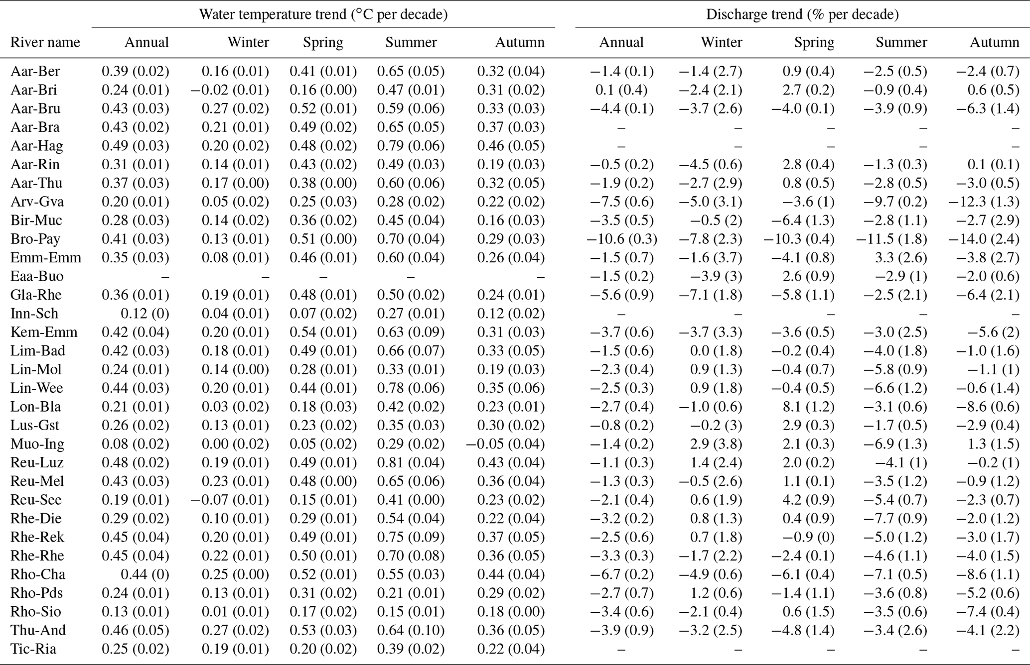
The annual and seasonal trends for stream temperature and discharge are presented for all catchments in Table A1 over the 1999–2018 period and in Table A2 over the 1979–2018 period. The trends for air temperature and precipitation are presented in Tables S4 and S5. Annual trends are computed with de-seasonalized daily time series, whereas seasonal trends are computed from annual means of each season, meaning that annual and seasonal trends should not be directly compared. This also explains why the standard error for the seasonal trend values is more important than that for the annual trend values (see discussion in Sect. 3.3).

Table A1 Water temperature (left section) and discharge (right section) annual and seasonal trends for all catchments presented in Table 1 over the 1999–2018 period. The numbers in parentheses indicate the standard error of the computed trends based on linear regression.

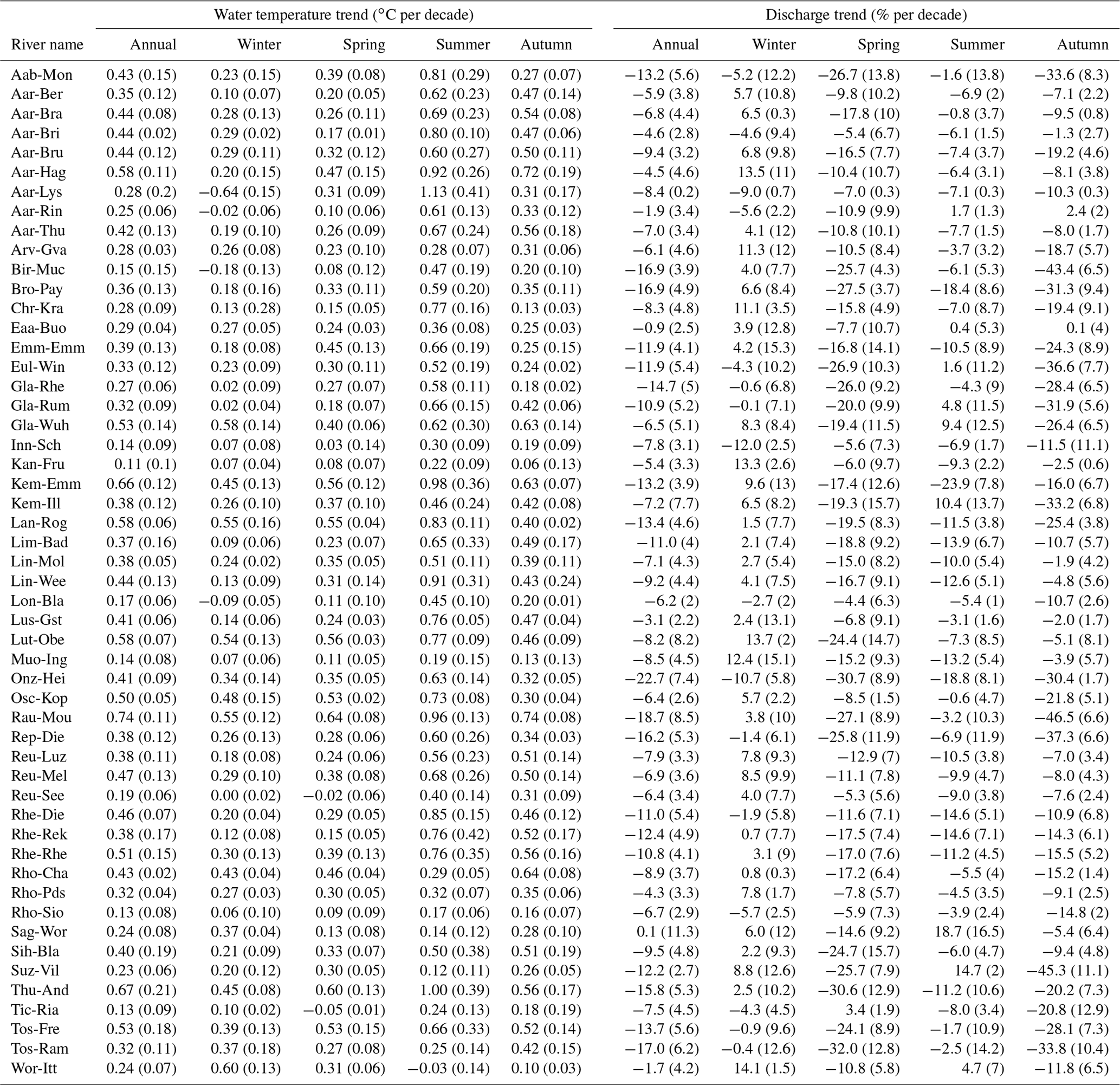
Table A2 Water temperature (left section) and discharge (right section) annual and seasonal trends for all catchments presented in Table 1 over the 1979–2018 period. The numbers in parentheses indicate the standard error of the computed trends based on linear regression.