A hybrid stochastic rainfall model that reproduces some important rainfall characteristics at hourly to yearly timescales

A novel approach to stochastic rainfall generation that can reproduce various statistical characteristics of observed rainfall at hourly to yearly timescales is presented. The model uses a seasonal autoregressive integrated moving average (SARIMA) model to generate monthly rainfall. Then, it downscales the generated monthly rainfall to the hourly aggregation level using the Modified Bartlett–Lewis Rectangular Pulse (MBLRP) model, a type of Poisson cluster rainfall model. Here, the MBLRP model is carefully calibrated such that it can reproduce the sub-daily statistical properties of observed rainfall. This was achieved by first generating a set of fine-scale rainfall statistics reflecting the complex correlation structure between rainfall mean, variance, auto-covariance, and proportion of dry periods, and then coupling it to the generated monthly rainfall, which were used as the basis of the MBLRP parameterization. The approach was tested on 34 gauges located in the Midwest to the east coast of the continental United States with a variety of rainfall characteristics. The results of the test suggest that our hybrid model accurately reproduces the first- to the third-order statistics as well as the intermittency properties from the hourly to the annual timescales, and the statistical behaviour of monthly maxima and extreme values of the observed rainfall were reproduced well.

1 Introduction and background

Most human and natural systems affected by rainfall react sensitively to temporal variability of rainfall across small (e.g. quarter-hourly) to large (e.g. monthly, yearly) timescales. Small-scale rainfall temporal variability influences short-term watershed responses such as flash floods (Reed et al., 2007) and subsequent transport of sediments (Ogston et al., 2000) and contaminants (Zonta et al., 2005). Large-scale rainfall temporal variability (Iliopoulou et al., 2016; Tyralis et al., 2018) influences long-term resilience of human–flood systems (Yu et al., 2017), human health (Patz et al., 2005), food production (Shisanya et al., 2011), and the evolution of human society (Warner and Afifi, 2014) and ecosystems (Borgogno et al., 2007; Fernandez-Illescas and Rodriguez-Iturbe, 2004).

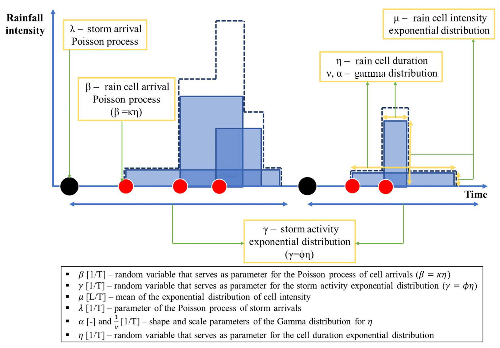
Figure 1 Schematic of the Modified Bartlett–Lewis Rectangular Pulse model. The blue area represents duration (width) and intensity (height) of each rain cell, respectively. The dashed line represents superposed sum of the rain cell intensities.

The risk posed by these impacts needs to be precisely assessed for the management of such systems, but the observed rainfall record is oftentimes “not” long enough for this purpose (Koutsoyiannis and Onof, 2001). Furthermore, the rainfall records do not exist when the risks need to be assessed for the future. For this reason, stochastic rainfall generators, which can create synthetic rainfall records with infinite length, have been frequently used to provide rainfall input data to the modelling studies for risk assessment.

The Poisson cluster rainfall generation model (Rodriguez-Iturbe et al., 1987, 1988) is one of the most widely applied stochastic rainfall generators. Figure 1 shows a schematic of the Modified Bartlett–Lewis Rectangular Pulse (MBLRP) model, which is a typical Poisson cluster rainfall model. The model assumes that a series of rainstorms (black circles) comprising a sequence of rain cells (red circles) arrives in time according to a Poisson process. The MBLRP model has six parameters of which a brief description is provided in the lower text box of Fig. 1.

As suggested by the figure, Poisson cluster rainfall models are designed to reflect the original spatial structure of rainstorms containing multiple rain cells (Austin and Houze Jr., 1972; Olsson and Burlando, 2002), so they are good at reproducing the first- to the third-order statistics of the observed rainfall at quarter-hourly to daily accumulation levels, as well as other hydrologically important statistics such as the proportion of non-rainy periods (Olsson and Burlando, 2002). The performance of the Poisson cluster rainfall models in reproducing the statistical properties of observed rainfall has been validated for various climates at numerous locations across the globe (Bo et al., 1994; Cameron et al., 2000; Cowpertwait, 1991; Cowpertwait et al., 2007; Derzekos et al., 2005; Entekhabi et al., 1989; Glasbey et al., 1995; Gyasi-Agyei and Willgoose, 1997; Gyasi-Agyei, 1999; Islam et al., 1990; Kaczmarska et al., 2014, 2015; Khaliq and Cunnane, 1996; Kim et al., 2013b, 2014, 2016, 2017a, b; Kossieris et al., 2015, 2016; Onof and Wheater, 1993, 1994a, b; Ritschel et al., 2017; Rodriguez-Iturbe et al., 1987, 1988; Smithers et al., 2002; Velghe et al., 1994; Verhoest et al., 1997; Wasko et al., 2015). For this reason, they have been widely applied to assess the risks exerted on human and natural systems such as floods (Paschalis et al., 2014), water availability (Faramarzi et al., 2009), contaminant transport (Solo-Gabriele, 1998), and landslides (Peres and Cancelliere, 2014, 2016; Thomas et al., 2018). Recently, Poisson cluster rainfall models have also been used to generate future rainfall scenarios under climate change (Kilsby et al., 2007; Burton et al., 2010; Fatichi et al., 2011).

In the meantime, Poisson cluster rainfall models have an intrinsic limitation derived from a fundamental model assumption. As described by Fig. 1, they generate the rainfall time series assuming that the rainstorms arrive according to a Poisson process, which assumes that rainstorm occurrences are independent. In addition, the rain cells in different storms are independent with each other. These model assumptions deprive the model of the ability to reproduce the long-term memory of rainfall that is often observed in reality (Marani, 2003).

Let us introduce some notation. The aggregated process Y^(h) at timescale h hours is defined in terms of the continuous time process Y by the following equation:

$$Y_i^{\left(h\right)}=\underset{\left(i-\mathrm{1}\right)h}{\overset{ih}{\int }}Y\left(t\right)\mathrm{d}t.$$

We can then write the variance at timescale nh as follows:

$$\begin{array}{ll}{\displaystyle }& {\displaystyle }{V}_{nh}=\mathrm{Var}\left(Y^{\left(nh\right)}\right)\\ {\displaystyle }& {\displaystyle }={\sum }_{i=\mathrm{1}}^n\mathrm{Cov}\left(Y_i^{\left(h\right)},Y_i^{\left(h\right)}\right)\\ {\displaystyle }& {\displaystyle }+{\sum }_{i=\mathrm{1}}^n{\sum }_{j=\mathrm{1},j\ne i}^n\mathrm{Cov}\left(Y_i^{\left(h\right)},Y_j^{\left(h\right)}\right)\\ {\displaystyle }& {\displaystyle }=n\mathrm{Var}\left(Y^{\left(h\right)}\right)+{\sum }_{i=\mathrm{1}}^n{\sum }_{j=\mathrm{1},j\ne i}^n\mathrm{Cov}\left(Y_i^{\left(h\right)},Y_j^{\left(h\right)}\right),\\ {\displaystyle }& {\displaystyle }\mathrm{since}\mathrm{Cov}\left(Y_i^{\left(h\right)},Y_j^{\left(h\right)}\right)=\mathrm{Cov}\left(Y_j^{\left(h\right)},Y_i^{\left(h\right)}\right)\\ \text{(1)}& {\displaystyle }& {\displaystyle }{V}_{nh}=n\mathrm{Var}\left(Y^{\left(h\right)}\right)+\mathrm{2}{\sum }_{i=\mathrm{1}}^n{\sum }_{j=\mathrm{1},j>i}^n\mathrm{Cov}\left(Y_i^{\left(h\right)},Y_j^{\left(h\right)}\right),\end{array}$$

where V_h is the variance of rainfall depths at scale h hours and $\mathrm{Cov}\left(\cdot ,\cdot \right)$ is the covariance operator between the two random variables.

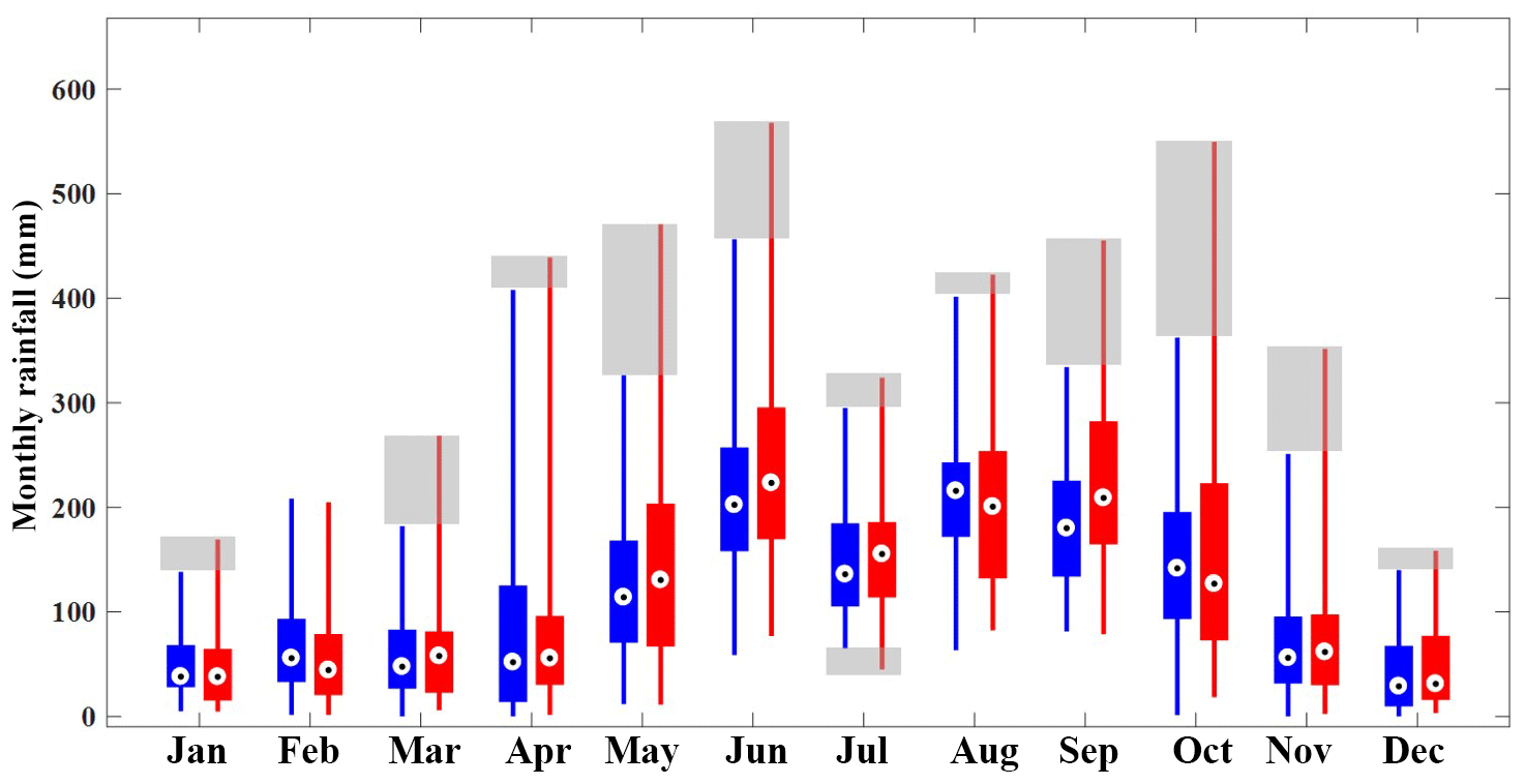
Figure 2 Box plots of the observed monthly rainfall at gauge NCDC-85663 in Florida, USA (red). The box plots of the synthetic monthly rainfall generated by the Modified Bartlett–Lewis Rectangular Pulse model at the same gauge are shown for reference (blue). Whiskers reach minimum and maximum values of monthly rainfall during the period between 1961 and 2010, and grey shaded boxes represent the discrepancy in the variability of the two monthly rainfall values.

The second term of the right-hand side of Eq. (1), which represents the rainfall correlation between individual records separated by (i−j) time steps of the time series of rainfall depths at scale h hours, is likely to be underestimated by the Poisson cluster rainfall model because it can only reproduce short-term memory in the rainfall signal through its model structure, i.e. through the clustering of rain cells. The degree of underestimation will increase as the correlation between the individual records ($Y_i^{\left(h\right)}$) of the observed rainfall time series increases and as the aggregation level n increases. This underestimation was consistently observed in the rainfall data of the United States (Kim et al., 2013a). If h=1 in Eq. (1), i.e. hourly rainfall, and n≅720 (24 h day${}^{-\mathrm{1}}\times \mathrm{30}$ days =720 h ≅1 month), the left-hand side of Eq. (1) will represent the variance of monthly rainfall, which can be represented on the vertical axis of the box plots in Fig. 2.

In Fig. 2, the red box plots represent the distribution of the monthly rainfall observed at gauge NCDC-85663 located in Florida, USA, during the period between 1961 and 2010. The blue box plots represent the variability of the monthly rainfall estimated from the 50 years of hourly synthetic rainfall data generated by the Modified Bartlett–Lewis Rectangular Pulse (MBLRP) model, a type of Poisson cluster rainfall generator. Here, the MBLRP model used the parameter set that was calibrated to reproduce the observed rainfall mean, variance, lag-1 auto-covariance, and proportion of dry periods at sub-daily aggregation intervals (1, 2, 4, 8, and 16 h), which is a typical practice of MBLRP model calibration (Rodriguez-Iturbe et al., 1987, 1988; Kim et al., 2013a). Note that the vertical lengths of the red box plots are greater than those of the blue box plots in general, which implies that the variability of the observed rainfall is systematically greater than that of the synthetic rainfall. The discrepancy between the two is shown as the grey shading in the figure. In addition, the monthly extreme values shown as the highest points of the lines are also underestimated by synthetic rainfall. This is, in particular, caused by the aforementioned limitations of the Poisson cluster rainfall models.

Considering that the management strategies of the water-prone human and natural systems may be governed by the few extreme rainfall values observed in the shaded domain of Fig. 2, the risk analysis based on the rainfall data generated by Poisson cluster rainfall models may miss system behaviour that is crucial for development of the management plans. As a matter of fact, other rainfall models have similar issues: they cannot reproduce the temporal variability of observed rainfall across all timescales (Paschalis et al., 2014). For example, Markov chains, alternating renewal processes, and generalized linear models can reproduce the variability only at timescales coarser than 1 day. Models based on autoregressive properties of rainfall are typically good at reproducing the observed rainfall variability only for a limited range of scales, for instance from 1 month to 1 or 2 years (Mishra and Desai, 2005; Modarres and Ouarda, 2014; Yoo et al., 2016).

Several studies discussed the need to use composite rainfall models to resolve this scale problem of rainfall models. Koutsoyiannis (2001) used two seasonal autoregressive models with different temporal resolution to generate two different time series referring to the same hydrologic process. Then, they adjusted the fine-scale time series using their novel coupling algorithm so that this series becomes consistent with the coarser-scale time series without affecting the second-order statistical properties. Menabde and Sivapalan (2000) combined the alternating renewal process with a multiplicative cascade model in which a multi-year rainfall time series generated by a Poisson-process-based model is disaggregated using a bounded random cascade model. Their model reproduced the observed scaling behaviour of extreme events very well up to 6 min of temporal resolution. Fatichi et al. (2011) developed a model that generates monthly rainfall using an autoregressive model and disaggregating the generated monthly rainfall using a Poisson cluster rainfall model. Their composite model showed improved performance in reproducing the rainfall interannual variability that the latter often fails to reproduce. Kim et al. (2013a) proposed a model where the Poisson cluster rainfall model is used to disaggregate the monthly rainfall that is randomly drawn from a Gamma distribution. They found that incorporating the observed rainfall interannual variability through their composite approach also helps reproduce the statistical behaviour of rainfall annual maxima and extreme values at timescales ranging from 1 to 24 h. Paschalis et al. (2014) introduced a composite model consisting of a Poisson cluster rainfall model or Markov chain model for large timescales and a multiplicative random cascade model for small timescales, which performed better than individual models across a wide range of scales at four different sites with distinct climatological characteristics.

This study proposes a composite rainfall generation model that can reproduce various statistical properties of observed rainfall at timescales ranging between 1 h and 1 year. First, the model generates the monthly rainfall time series using a seasonal autoregressive integrated moving average (SARIMA) model. Then, it downscales the generated monthly rainfall time series to the hourly aggregation level using a Poisson cluster rainfall model. Compared to the previous studies with similar methodology (Fatichi et al., 2011; Paschalis et al., 2014), our model has a novelty in that (i) it models the monthly rainfall values so as to generate monthly statistics that will serve to calibrate the MBLRP model, and (ii) each of the generated individual monthly rainfall values are downscaled using month-specific MBLRP model parameter sets that reflect the complex correlation structure of various rainfall statistics at fine timescales such as mean, variance, covariance, and proportion of dry periods, which existing composite approaches that are not based on Poisson cluster rainfall models showed limitations in reproducing, especially at sub-daily scale. This distinctive approach of our model enables an accurate reproduction of the first- to the third-order statistics as well as the proportion of dry periods from the hourly to the annual timescale, and the statistical behaviour of monthly maxima and extreme values of the observed rainfall is well reproduced.

2 Study area

Figure 3 shows the study area, which encompasses a region from the Midwest to the east coast of the continental United States. We used the National Climatic Data Centre (NCDC) hourly rainfall data observed at 34 gauge locations (triangles in Fig. 3) for the period between 1981 and 2010. The study area has a variety of rainfall characteristics (Kim et al., 2013b). The northern, middle, and the southern part of the study area are classified as humid continental (warm summer), humid continental (cool summer), and humid subtropical climate, respectively, according to the Köppen climate classification (Köppen, 1900; Kottek, 2006). The annual rainfall of the study area varies from 750 to 1500 mm.

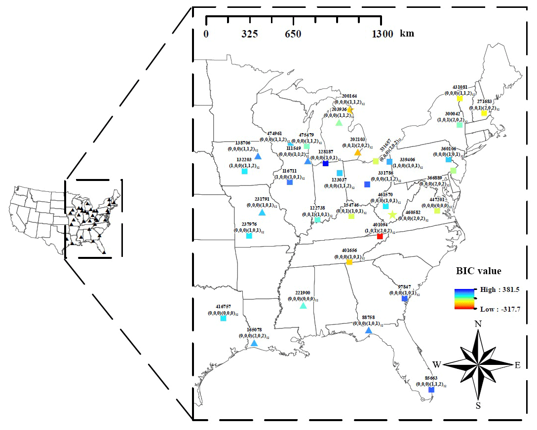
Figure 3 Study area and 34 NCDC hourly rainfall gauges. The label of the markers is presented in the following format: xxxxxx($i,j,k$)($x,y,z$)₁₂, where xxxxxx represents the NCDC gauge ID; ($i,j,k$) represent the orders of the autoregressive, differencing, and moving average terms of the SARIMA model; and ($x,y,z$) represent the orders of the seasonal autoregressive, differencing, and moving average terms of SARIMA model. The colour of the markers represent the Bayesian information criterion (BIC) value of the SARIMA model. The lower BIC indicates more parsimonious parameterization, larger likelihood, or both. Model description of SARIMA is detailed in Sect. 3.1.

3 Methodology

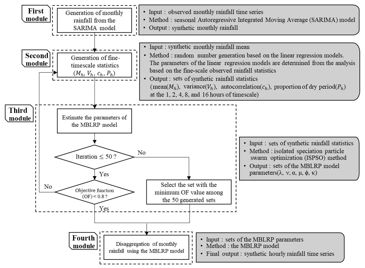
Figure 4 describes the model structure of this study. The model is composed of four distinct modules. The first module generates the monthly rainfall. The second module generates the fine-scale (1 to 16 h) rainfall statistics corresponding to each of the generated monthly rainfall values in the first module. The third module estimates the parameters of the MBLRP model based on the fine-scale rainfall statistics generated by the second module. As a result of this process, each of the generated monthly rainfall values is coupled with the MBLRP parameter set reflecting its fine-scale statistical characteristics. The fourth module downscales each of the monthly rainfall values using the MBLRP model based on the parameters obtained in the third module.

Figure 4 The four different modules of the model of this study.

3.1 Monthly rainfall generation

We applied a seasonal autoregressive integrated moving average (SARIMA) model to generate monthly rainfall. Generation of monthly rainfall based on autoregressive relationships has been widely applied due to its parsimonious nature (Mishra and Desai, 2005) and was proven to successfully reproduce the first to the third-order statistics of the observed rainfall at monthly timescales (Delleur and Kavvas, 1978; Katz and Skaggs, 1981; Ünal et al., 2004; Mishra and Desai, 2005). Furthermore, some recent models assuming an autoregressive process (Langousis and Koutsoyiannis, 2006; Koutsoyiannis, 2010; Efstratiadis et al., 2014; Dimitriadis and Koutsoyiannis, 2015, 2018) succeeded in reproducing the various statistical properties of the observed rainfall over a wider range of scales. Rainfall data of different stations have different temporal persistence, so we applied the SARIMA model with different autoregressive (p), differencing (d), and moving average terms (q) to different stations. The choice of the optimal model for each station was determined through the following processes: First, a model structure of SARIMA($p,d,q$)($P,D,Q$)_m is assumed, where P,D, and Q represent the numbers of seasonal autoregressive, differencing, and moving average terms, respectively, and m represents the number of periods (here, months) in each season – here m=12. Second, the parameters of the SARIMA model are determined through the method of maximum likelihood. Third, the Bayesian information criterion (BIC) are calculated for the fitted SARIMA model. Lastly, the first to third steps are repeated for a combination of different values of p ($\mathrm{0}\le p\le \mathrm{2}$), d ($\mathrm{0}\le d\le \mathrm{2}$), q ($\mathrm{0}\le q\le \mathrm{2}$), P ($\mathrm{0}\le P\le \mathrm{2}$), D ($\mathrm{0}\le D\le \mathrm{2}$), and Q ($\mathrm{0}\le Q\le \mathrm{2}$), and the model structure with the lowest BIC is selected for the station. Therefore, a total of 729 (=3⁶) SARIMA model structures were tested to obtain the optimal model for a station. The selected model structure and the BIC values were shown in Fig. 3. Through this process, we generated 200 years of monthly rainfall for the 34 gauges.

3.2 Generation of fine-timescale rainfall statistics

The second module generates the fine-timescale statistics corresponding to each monthly rainfall value generated through the SARIMA model. These synthetic fine-timescale statistics will later be used for the calibration of the MBLRP model to downscale the monthly rainfall to the hourly level. In so doing we first consider the monthly rainfall, when divided by the number of days in the month times 24, as providing us with an estimate of the mean hourly rainfall for that particular month. Then, this estimated mean hourly rainfall is provided as the input variable of the module that generates the statistics needed to fit the MBLRP model, namely the mean, variance, autocorrelation coefficient, and the proportion of dry periods at 1, 2, 4, 8, and 16 h aggregation intervals, as described in Fig. 5. In this process, the module employs the information obtained from univariate regression analyses between the fine-scale statistics of the observed rainfall (Fig. 6) and the mathematical formulae relating rainfall variance and auto-covariance at different timescales (Eq. 4), as explained below.

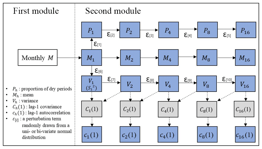
Figure 5 Schematic of the algorithm to generate fine-timescale rainfall statistics. The statistics in the blue boxes are used to calibrate the MBLRP model and the statistics in grey boxes are used to estimate the lag-1 autocorrelation.

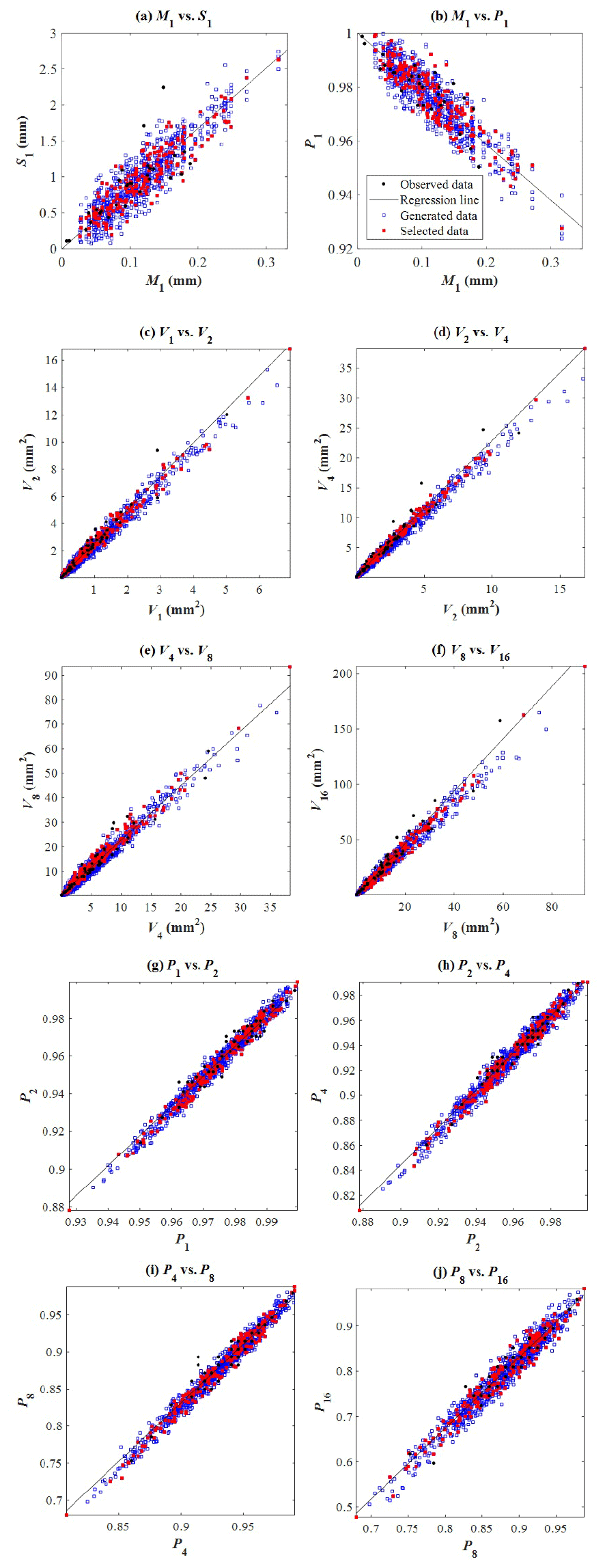
Figure 6 Linear relationship between various fine-timescale statistics of the rainfall observed for the month of July of different years at gauge NCDC-200164 (black dots). The solid black line represents the least-squares regression line. Based on this regression relationship, a set of the 20 fine-timescale statistics are generated, which are immediately used as the basis of the MBLRP model parameter calibration. If the objective function of the parameter calibration corresponding to the generated set is greater than a given threshold, the set is rejected (blue squares), and only the set with the objective function lower the threshold value is chosen (red squares).

Figure 5 shows a schematic of the second module. In the figure, M_h, S_h, $V_h,c_h\left(\mathrm{1}\right)=C_h\left(\mathrm{1}\right)/V_h$, and P_h in each rectangle represents the rainfall mean, standard deviation, variance, lag-1 autocorrelation, and proportion of dry periods at a timescale of h hours, respectively. The statistic connected to each solid arrow head is stochastically generated based on its linear relationship to the one connected to the tail of the same arrow. In other words, the following equation is used:

$$\begin{array}{}\text{(2)}& Y=a_{\left[i\right]}X+b_{\left[i\right]}+{\mathit{\epsilon }}_{\left[i\right]},\end{array}$$

where Y is the variable being generated, and X is the variable being used as the basis of the generation. Here, the variables X and Y can be substituted by any combination of two variables connected by the solid arrow; a_[i] and b_[i] are the parameters of the regression analysis, and ε_[i] is a random number drawn from the normal distribution ${\mathit{\epsilon }}_{\left[i\right]}\sim N\left(\mathrm{0},{\mathit{\sigma }}_{\left[i\right]}^{\mathrm{2}}\right)$ fitted to the residuals of the regression analysis. Here, these three parameters are estimated from the univariate regression analysis relating the two variables observed during a given calendar month over multiple years as shown by black dots in each plot of Fig. 6, which shows the linear relationship between the rainfall statistics observed at gauge NCDC-200164 (yellow star mark in Fig. 3) during the month of July of different years.

The linear relationships were also identified at all other gauges investigated. This is a secondary yet significant finding of this study: a simple linearity can accurately express the relationship between the variables reflecting such chaotic and dynamic interactions occurring in natural phenomena concerning rainfall. Also note that the linearity established here applies only to sub-daily timescales. For example, a power-law may better express the relationship between the mean and standard deviation at daily scale (Sotiriadou et al., 2016).

Consider, for example, statistic M₁ which is connected to $V_{\mathrm{1}}(=S_{\mathrm{1}}^{\mathrm{2}})$ through the solid arrow in the figure, which means that the variance of 1 h rainfall ($V_{\mathrm{1}}=S_{\mathrm{1}}^{\mathrm{2}}$) is stochastically generated using its relationship to 1 h rainfall mean (M₁) (scatter of black dots in Fig. 6a) using the following formula:

$$\begin{array}{}\text{(3)}& {\displaystyle }& {\displaystyle }{S}_{\mathrm{1}}=a_{\left[\mathrm{6}\right]}{M}_{\mathrm{1}}+{\mathit{\epsilon }}_{\left[\mathrm{6}\right]},\text{(4)}& {\displaystyle }& {\displaystyle }{V}_{\mathrm{1}}=S_{\mathrm{1}}^{\mathrm{2}},\end{array}$$

where subscripts with square brackets are used for the residuals so as to avoid confusion with the timescale, and where a_[6] is the coefficient determined from the regression analysis (note that the constant term is zero here since, trivially, S₁=0 when M₁=0), and ε_[6] is a random number drawn from a normal distribution: ${\mathit{\epsilon }}_{\left[\mathrm{6}\right]}\sim N(\mathrm{0},{\mathit{\sigma }}_{\left[\mathrm{6}\right]}^{\mathrm{2}})$.

Similar principles can be applied to the remaining statistics connected through solid arrows in Fig. 5. The black dots in Fig. 6 shows the linear relationship between the rainfall statistics observed at gauge NCDC-200164 (star mark in Fig. 3) during the month of July of different years.

The statistic connected to the dashed arrow head is calculated based on the ones connected to the tail of the same arrow using the mathematical (deterministic) relationship connecting these variables (Eq. 4). For instance, in Fig. 5, V₁ and V₂ are connected to C₁(1) through a dashed arrow, which means that C₁(1) is derived from V₁ and V₂. The following equations establish the relationship between the variances at timescales h and 2 h from which we shall obtain the relationship between V₁ and V₂:

$$\begin{array}{ll}{\displaystyle }\mathrm{Var}\left(Y_i^{\left(\mathrm{2}\mathrm{h}\right)}\right)& {\displaystyle }=\mathrm{Var}\left(Y_{\mathrm{2}i-\mathrm{1}}^{\left(h\right)}\right)+\mathrm{Var}\left(Y_{\mathrm{2}i}^{\left(h\right)}\right)\\ {\displaystyle }& {\displaystyle }+\mathrm{2}\mathrm{Cov}\left(Y_{\mathrm{2}i-\mathrm{1}}^{\left(h\right)},Y_{\mathrm{2}i}^{\left(h\right)}\right).\end{array}$$

Or, in simplified notation:

$$V_{\mathrm{2}\mathrm{h}}=\mathrm{2}{V}_h+\mathrm{2}{C}_h\left(\mathrm{1}\right).$$

The autocorrelation lag-k is $c_h\left(k\right)=C_h\left(k\right)/V_h$, so, for k=1 and h=1 h, we obtain the following relation:

$$\begin{array}{}\text{(5)}& c\left(\mathrm{1}\right)={\displaystyle \frac{V_{\mathrm{2}}}{\mathrm{2}{V}_{\mathrm{1}}}}-\mathrm{1}.\end{array}$$

If we estimate the lag-1 autocorrelation using standard estimators of the terms in the right-hand side of this relation, i.e. by using $\frac{\widehat{V_{\mathrm{2}}}}{\mathrm{2}\widehat{V_{\mathrm{1}}}}-\mathrm{1}$, how good is the estimation likely to be? Figure 7 compares this estimator with the standard estimator $\widehat{c\left(\mathrm{1}\right)}$ of the autocorrelation.

Figure 7 (a) Comparison of estimator $\widehat{c\left(\mathrm{1}\right)}$ (horizontal axis) with estimator $\frac{\widehat{V_{\mathrm{2}}}}{\mathrm{2}\widehat{V_{\mathrm{1}}}}-\mathrm{1}$ (vertical axis) of the autocorrelation lag-1 of hourly rainfall. (b) The histogram of the discrepancies between these two estimators at gauge NCDC-200164.

Figure 7a reveals that there exist discrepancies between the true c(1) and its estimator ($\widehat{c\left(\mathrm{1}\right)})$, which are known to primarily depend on the sample size (Dimitriadis and Koutsoyiannis, 2015; Koutsoyiannis, 2016). Using the discrepancies ε between these two estimators which are approximately normally distributed as shown in Fig. 7b, i.e. $\mathit{\epsilon }\sim N\left(\mathrm{0},{\mathit{\sigma }}^{\mathrm{2}}\right)$, we therefore estimate the autocorrelation lag-1 of hourly rainfall using $\frac{\widehat{V_{\mathrm{2}}}}{\mathrm{2}\widehat{V_{\mathrm{1}}}}-\mathrm{1}+\mathit{\epsilon }$.

$$\begin{array}{}\text{(6)}& {\displaystyle }& {\displaystyle }{V}_{\mathrm{2}}={\mathrm{a}}_{\left[\mathrm{7}\right]}{V}_{\mathrm{1}}+{\mathit{\epsilon }}_{\left[\mathrm{7}\right]}\text{(7)}& {\displaystyle }& {\displaystyle }{V}_{\mathrm{4}}={\mathrm{a}}_{\left[\mathrm{8}\right]}{V}_{\mathrm{2}}+{\mathit{\epsilon }}_{\left[\mathrm{8}\right]}\end{array}$$

From Eq. (6), it is clear that the term ε_[7] is dependent upon the hourly autocorrelation (lag-1) coefficient, and similarly therefore that ε_[8] in Eq. (7) is dependent upon the 2-hourly (lag-1) autocorrelation coefficient.

The autocorrelations at various timescales are known to be correlated with each other (Kim et al., 2013a, 2014), which means that ε_[7] and ε_[8] should be correlated with each other. Figure 8a shows the bivariate probability density function of these two variables at gauge NCDC-200164 for the month of September. Figure 8b shows the colour map of the correlation coefficient between different ε_[i]s. This study developed bivariate probability density functions for consecutively numbered random variables ε, i.e. ε_[i] and ε_[i+1] (for i ranging from 1 to 4 and 6 to 9 respectively – see Fig. 5). These were then used to sample values of ε_[i+1] conditional upon ε_[i]. This procedure in effect assumes that a Markov structure governs the sequences ${\left\{{\mathit{\epsilon }}_{\left[i\right]}\right\}}_{i=\mathrm{1},\mathrm{\dots },\mathrm{5}}$ and ${\left\{{\mathit{\epsilon }}_{\left[i\right]}\right\}}_{i=\mathrm{6},\mathrm{\dots },\mathrm{10}}$. The bivariate probability density functions were developed using the Gaussian Copula and its parameters are determined using the maximum likelihood method.

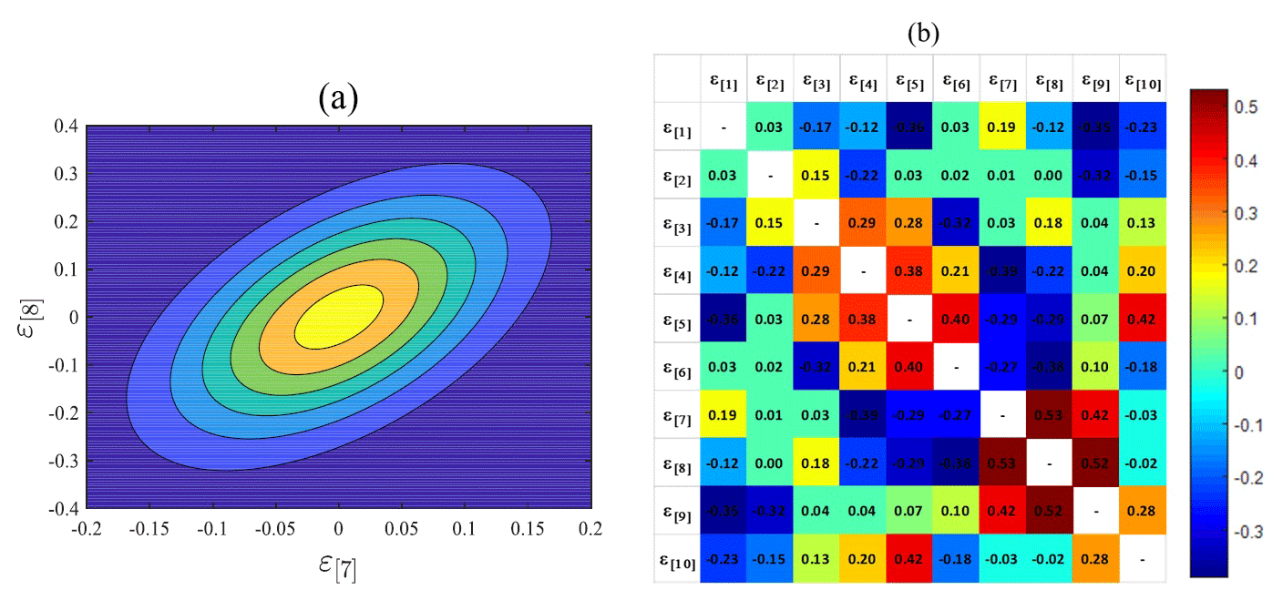
Figure 8 (a) Relationship between ε_[7] and ε_[8] and the fitted bivariate distribution. (b) Color map of the correlation coefficient between different ε_[i]s at gauge NCDC-200164 on September.

Residual terms (ε_[i+1]) are thus generated using the conditional distribution:

$$\begin{array}{}\text{(8)}& f_{{\mathit{\epsilon }}_{[i+\mathrm{1}]}}(y\left|{\mathit{\epsilon }}_{\left[i\right]}=x)=\right.{\displaystyle \frac{f_{{\mathit{\epsilon }}_{\left[i\right]},{\mathit{\epsilon }}_{[i+\mathrm{1}]}}(x,y)}{f_{{\mathit{\epsilon }}_{\left[i\right]}}\left(x\right)}},\end{array}$$

where $i=\mathrm{1},\mathrm{2},\mathrm{3},\mathrm{4},\mathrm{6},\mathrm{7},\mathrm{8}$; 9; $f_{{\mathit{\epsilon }}_{[i+\mathrm{1}]}}(y\left|{\mathit{\epsilon }}_{\left[i\right]}=x)\right.$ is the probability density function of ε_[i+1] conditional upon ε_[i]=x; and $f_{{\mathit{\epsilon }}_{\left[i\right]},{\mathit{\epsilon }}_{[i+\mathrm{1}]}}$ is the bivariate distribution function of ε_[i] and ε_[i+1].

As a result of this process, a total of 20 rainfall statistics at fine timescales (mean; variance; lag-1 autocorrelation; and proportion of dry period at 1-, 2-, 4-, 8-, and 16-hourly aggregation interval) are sampled using these conditional distributions and the individual monthly rainfall that is generated by the SARIMA model.

3.3 MBLRP model parameter estimation

In this process, each of the monthly rainfall values generated by the SARIMA model is coupled with one set of six MBLRP model parameters that define the random nature of rainstorm and rain cell arrival frequency, and the intensity and duration of rain cells (Fig. 1).

In this study, the parameters of the MBLRP model were determined such that the rainfall statistics of the generated rainfall resemble the 20 fine-scale rainfall statistics that were coupled with the monthly rainfall generated by the SARIMA model. The Isolated-Speciation Particle Swarm Optimization (ISPSO; Cho et al., 2011) algorithm was employed to identify a set of parameters that minimizes the following objective function:

$$\begin{array}{}\text{(9)}& \mathrm{OF}={\sum }_{i=\mathrm{1}}^{\mathrm{20}}{w}_i\cdot {\left[\mathrm{1}-{\displaystyle \frac{F_i(\mathit{\lambda },\mathit{\nu },\mathit{\alpha },\mathit{\mu },\mathit{\varphi },\mathit{\kappa })}{f_i}}\right]}^{\mathrm{2}}.\end{array}$$

F_i is the ith statistic of the synthetic rainfall time series (e.g. mean of hourly rainfall, standard deviation of 4-hourly rainfall). The mathematical formulae for the F_is were derived by Rodriguez-Iturbe et al. (1988) as a function of the six parameters ($\mathit{\lambda },\mathit{\nu },\mathit{\alpha },\mathit{\mu },\mathit{\varphi },\mathit{\kappa }$); f_i is the ith generated statistic, and w_i the weighting factor given to the ith rainfall statistic depending on the use of the synthetic rainfall time series (Kim and Olivera, 2011). Here, it should be noted that a time step with rainfall less than 0.5 mm was considered dry when the proportion of non-rainy periods was calculated because small rainfall values are known to distort the “true” proportion of non-rainy periods exerting an adverse effect on calibration process (Kim et al., 2016; Cross et al., 2018).

It is noteworthy that Module 2 may fail to generate a realistic set of fine-scale rainfall statistics due to the complex interdependencies between them. The unrealistic fine-scale rainfall statistics cannot be represented by the MBLRP model that reflects the original spatial structure of rainfall in reality, which entails poorly calibrated model parameters with the high objective function value of Eq. (8). To exclude the poorly calibrated parameter sets caused by the unrealistic fine-scale rainfall statistics generated by Module 2, we repeated the process of Module 2 and Module 3 until the objective function value of Eq. (8) becomes lower than a given threshold value (0.8 in this study). If the algorithm fails to find the parameter set after 50 repetitions, the parameter set with the lowest objective function value is chosen. Figure 4 describes this filtering process, and the red squares in Fig. 6 show the chosen parameter sets.

3.4 Downscaling of monthly rainfall using the MBLRP model

The MBLRP model was used to downscale the monthly rainfall to the hourly aggregation level. First, the MBLRP model generates the hourly rainfall time series using the parameter set for the monthly rainfall being downscaled. Second, the discrepancy between the fine-timescale statistics generated by the second module of the model (Fig. 5) and the statistics of the synthetic hourly rainfall time series generated by the MBLRP model is calculated using the following formula:

$$\begin{array}{}\text{(10)}& D^j={\sum }_{i=\mathrm{1}}^{\mathrm{20}}{\left[{\displaystyle \frac{S_i^j-f_i}{R_i}}\right]}^{\mathrm{2}},\end{array}$$

where D^j is the discrepancy between the generated statistics and statistics of jth synthetic hourly rainfall time series. $S_i^j$ is the ith statistic of jth time series and R_i is the difference between maximum and minimum values of $S_i^j$ about the ith statistic.

Third, the first and the second processes are repeated 300 times. Then the synthetic hourly rainfall time series with the lowest discrepancy value is chosen. Finally, we repeated the entire process 200 times to obtain 200 synthetic hourly rainfall time series for each of the generated monthly rainfall values.

3.5 Validation for ungauged periods

One of the primary purposes of the stochastic rainfall model is to provide synthetic rainfall for the ungauged periods, which can be the periods of missing data or future periods. For this reason, we separated the period of model calibration and validation at some gauge locations (square marks in Fig. 2) where the record length of each period is sufficiently long (60+ years). Then, we tested our model not only based on the statistics of the calibration period (1981–2010) but also based on the validation period (1951–1980).

4 Result

4.1 Monthly rainfall statistics reproduction

Figure 9 compares the mean, variance, lag-1 autocorrelation, and skewness of the monthly rainfall time series generated by the SARIMA model (x axis) to those of the observed monthly rainfall time series (y axis). Each scatter represents one rainfall gauge. For the calibration period (1981–2010), the first- and the second-order moments were reproduced accurately with the coefficient of determination ranging from 0.69 to 0.95. Skewness was reproduced fairly well with the coefficient value of 0.36. For the validation period (1951–1980), mean and variance were reproduced, but not lag-1 autocorrelation and skewness. However, this discrepancy cannot be attributed solely to the limitations in the model because the discrepancy in each plot of Fig. 9 directly results from the differences between the statistics of the calibration and validation periods. In other words, had the statistics of the calibration period been similar to those of the validation period, we would have expected similar performance for both periods, and vice versa.

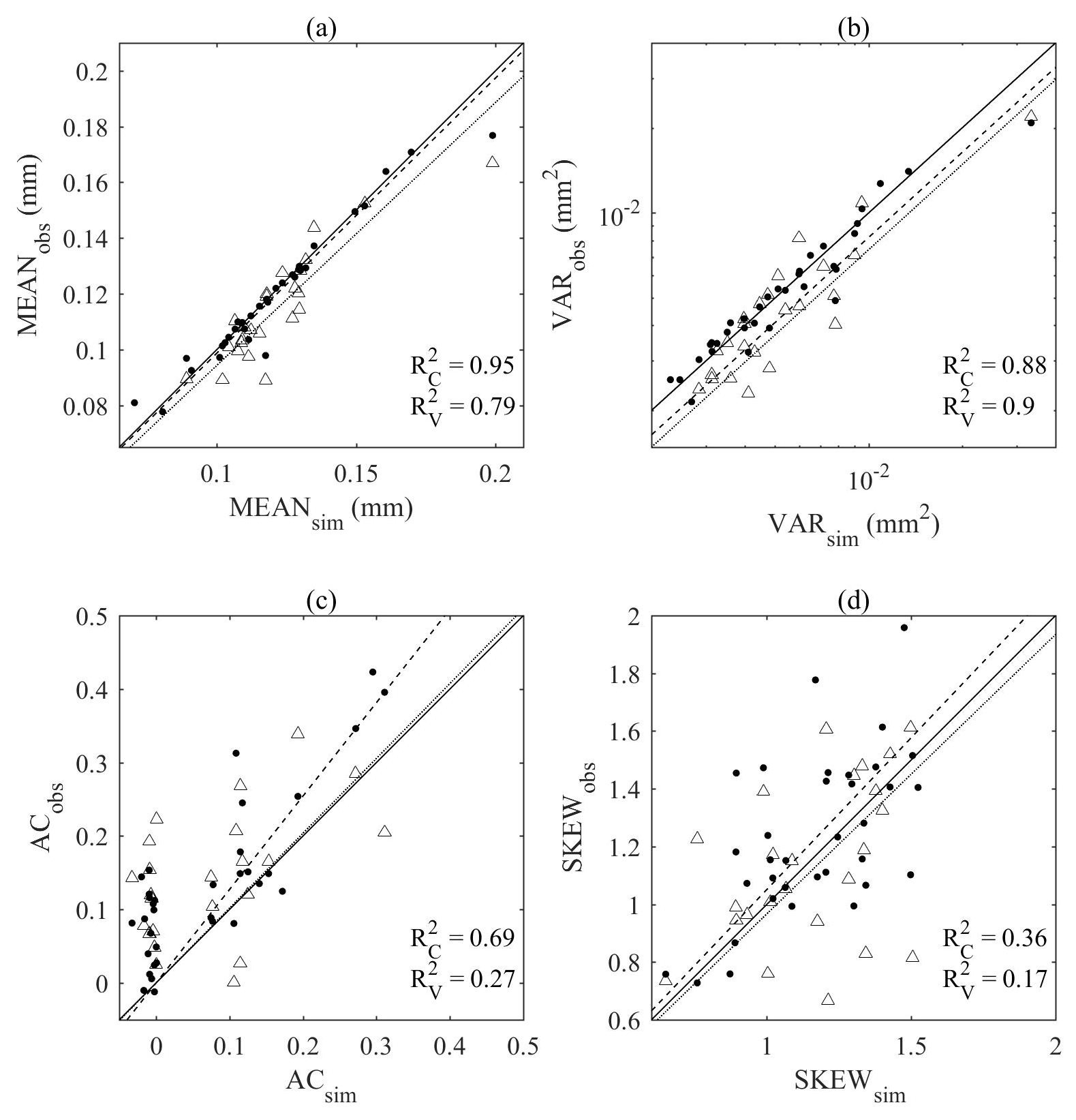
Figure 9 Comparison of (a) mean, (b) variance, (c) lag-1 autocorrelation, and (d) skewness of the synthetic (x) and observed (y) monthly rainfall. Filled circles (dashed line) and hollow triangles (dotted line) correspond to the calibration (1981–2010) and validation period (1951–1980) respectively.

4.2 Reproduction of large-scale rainfall variability

Figure 10 shows the behaviour of the rainfall variance varying with temporal aggregation intervals between 1 h and 1 year at gauge NCDC-122738. The behaviour corresponding to the observed calibration (black, 1981–2010), observed validation (green, 1951–1980), MBLRP (blue) and our hybrid model (red) is shown together. In addition, the behaviour based on the two-parameter generalized Hurst–Kolmogorov process (grey, GHK hereafter; Koutsoyiannis, 2016; Dimitriadis and Koutsoyiannis, 2018) is shown together. The good fit between the GHK behaviour (grey) and the observed behaviour (black and green) indicates that the observed rainfall has a clear long-term persistency, which is also a feature of all 34 NCDC gauges. While our model successfully reproduces the rainfall variance across the timescale, the MBLRP model is successful in reproducing the rainfall variance only at the hourly accumulation level. This reflects the fact that Poisson cluster rainfall models are not designed to preserve the rainfall persistence at the aggregation interval that is greater than the typical model storm duration, i.e. a few hours. See Fig. 1 for example. Within the duration of one storm, rainfall at different time steps may be similar insofar as a portion of it is from the same rain cell. However, the rainfall within one storm is independent of the rainfall within another storm. Therefore, it is natural that Poisson cluster rainfall models tend to underestimate the observed rainfall variance (which reflects the covariance structure – see Eq. 1) at timescales exceeding the rainstorm duration. Kim et al. (2013b), when mapping the average model storm duration across the continental United States using Eq. (11), showed that the model storm duration of the MBLRP model ranges from approximately 2 to 100 h, so it is not only at the annual scale, but already at the scale of several hours (depending upon the location) that the variability may be underestimated by the MBLRP model.

$$\begin{array}{ll}{\displaystyle }& {\displaystyle }\mathrm{Average}\mathrm{storm}\mathrm{duration}\left(\mathrm{h}\right)\cong \\ \text{(11)}& {\displaystyle }& {\displaystyle }{\displaystyle \frac{\mathrm{1}}{\mathit{\varphi }\frac{\mathit{\alpha }}{\mathit{\nu }}\left[\mathrm{1}+\mathit{\varphi }\left(\mathit{\kappa }+\mathit{\varphi }\right)-\frac{\mathrm{1}}{\mathrm{4}}\mathit{\varphi }\left(\mathit{\kappa }+\mathit{\varphi }\right)\left(\mathit{\kappa }+\mathrm{4}\mathit{\varphi }\right)+\frac{\mathrm{1}}{\mathrm{72}}\mathit{\varphi }\left(\mathit{\kappa }+\mathit{\varphi }\right)(\mathrm{4}{\mathit{\kappa }}^{\mathrm{2}}+\mathrm{27}\mathit{\kappa }\mathit{\varphi }+\mathrm{72}{\mathit{\varphi }}^{\mathrm{2}}\right]}}.\end{array}$$

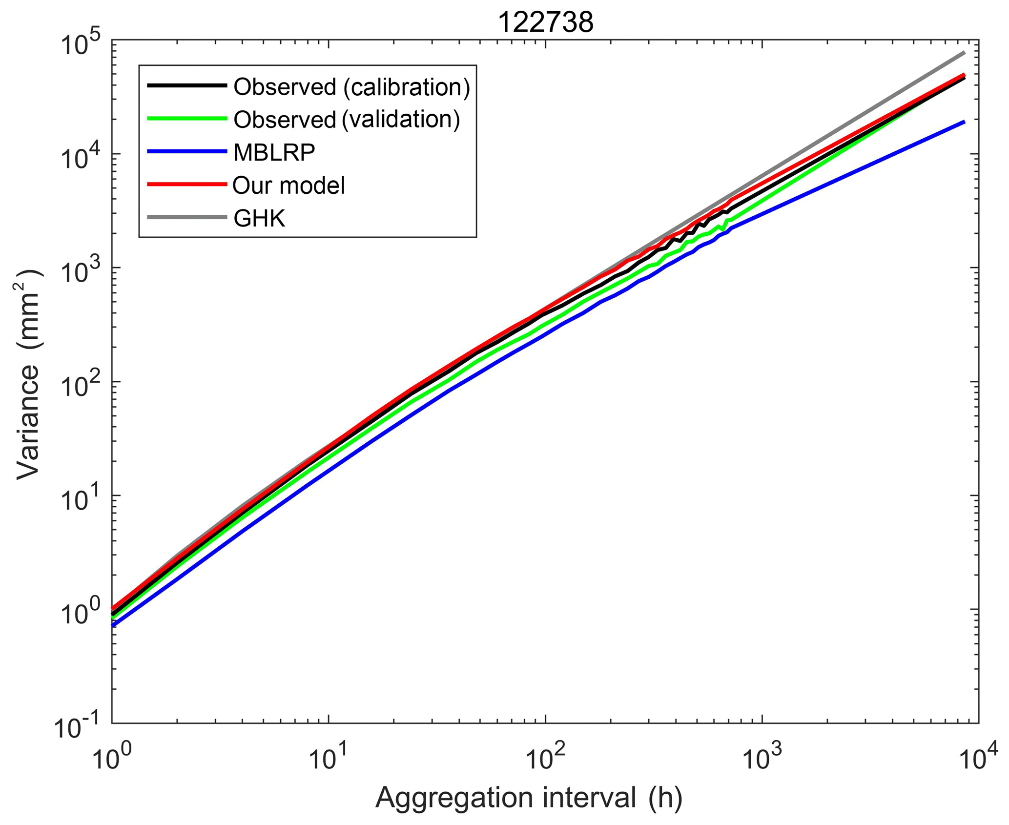
Figure 10 Behaviour of the rainfall variance with regard to the aggregation interval of rainfall time series at gauge NCDC-122738. The behaviour corresponding to the observed calibration (black, 1981–2010), observed validation (green, 1951–1980), MBLRP (blue) and our hybrid model (red) is shown together.

A similar trend as exhibited in Fig. 11 was observed at all of the 34 gauges. Figure 11 compares the variance of the synthetic (x) and observed (y) rainfall time series at yearly (purple), monthly (red), 15-daily (yellow), weekly (blue), and 32-hourly (green) aggregation levels. The comparison of the variance at the finer timescale is carried out in the following section.

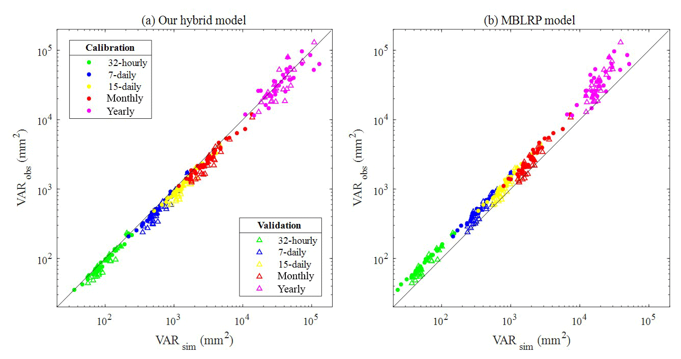
Figure 11 (a) Comparison of the large-scale rainfall variance of the rainfall generated by our hybrid model (x) and the observed rainfall (y). (b) Comparison of the large-scale rainfall variance of the rainfall generated by the traditional MBLRP model (x) and the observed rainfall (y). The different colours of the scatter correspond to the different aggregation interval of rainfall time series. Filled circles and hollow triangles correspond to the calibration and validation periods respectively.

As indicated by the concentration of the scatters above the 1:1 line in Fig. 11b, the traditional MBLRP model systematically underestimates the variability at timescales greater than 32 h. Our model did not show any bias in this range of large timescales as shown in Fig. 11a.

4.3 Reproduction of sub-daily rainfall statistics

Figure 12 compares the mean, variance, lag-1 autocorrelation, skewness, and the proportion of dry periods of the synthetic (x) and observed (y) rainfall time series at hourly to 16-hourly aggregation levels. Here, we discuss the first- to third-order moments only (i.e. mean, variance, autocorrelation, and skewness) because of their relatively greater importance compared to the higher moments (Kim and Olivera, 2011; Dimitriadis and Koutsoyiannis, 2018). Each scatter plot represents the statistics at a given gauge for a given calendar month. The colours of the points on the plots represent the calendar months. In each plot, the coefficient of determination (R²) of the linear regression between the two variables is shown. All five statistics were accurately reproduced across various sub-daily timescales with R² equal to 0.98 (mean), and varying between the following limits for the other statistics: 0.90 and 0.93 (variance), 0.58 and 0.93 (lag-1 autocorrelation), 0.44 and 0.89 (skewness), and 0.67 and 0.85 (proportion of dry periods) for the calibration period (Fig. 12a). Similar ranges of coefficient of determination were obtained for the validation period (Fig. 12b).

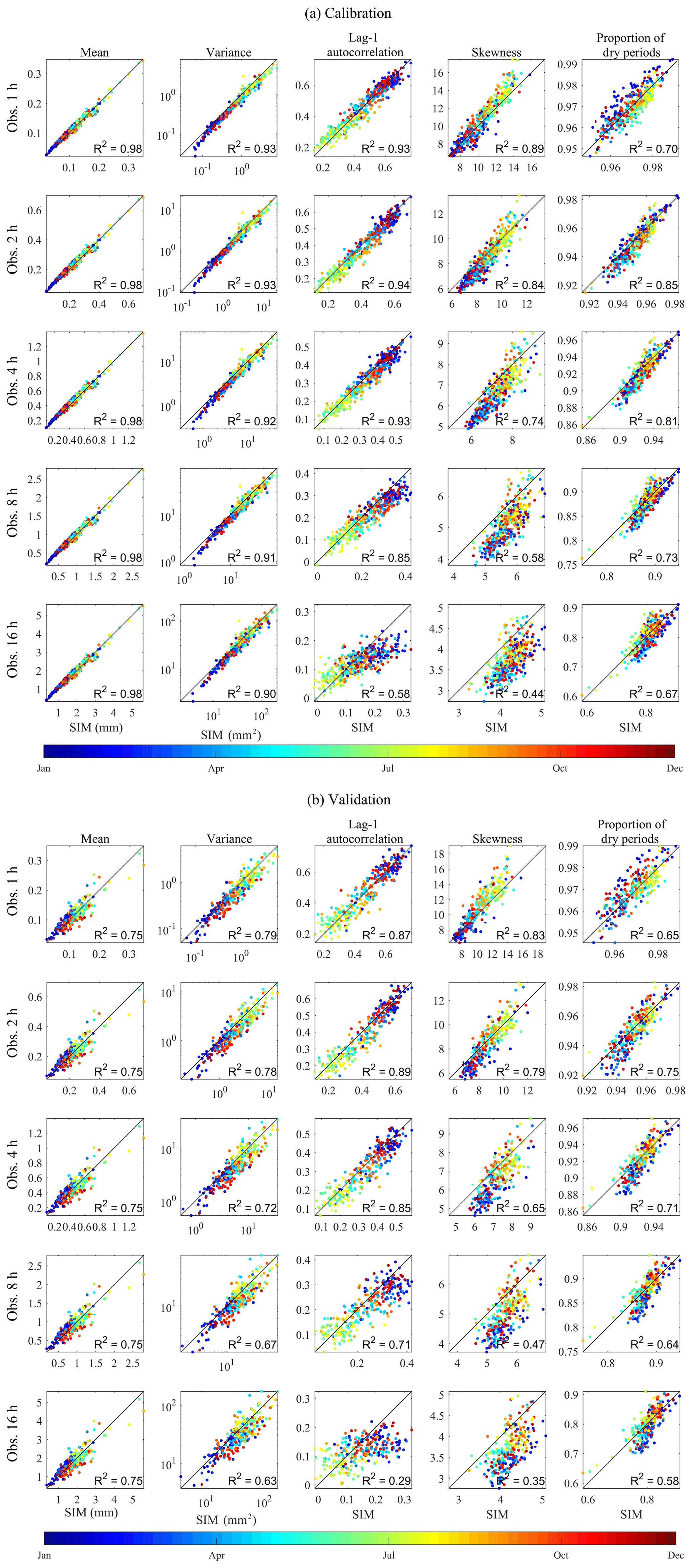
Figure 12 Comparison of the statistics of the synthetic (x) and observed (y) rainfall time series at sub-daily timescales. The colour of the dots represents the statistics of each calendar month. The results of (a) the calibration period (1981–2010) and (b) the validation period (1951–1980) are shown.

4.4 Reproduction of extreme values and distribution of annual maxima

The scatters in Fig. 13 compare the 20-, 50-, 100-, and 200-year rainfall estimated from the observed rainfall (x) and the synthetic rainfall (y) generated by the hybrid model (red) and the MBLRP model (blue) at hourly to daily timescales. The generalized extreme-value (GEV) distribution was used to model the distribution of the annual maxima, and the three parameters of the GEV distribution were determined using the method of L moments. Here, we separated the analysis for each calendar month, so we have 12 sets of extreme rainfall distributions corresponding to each gauge station. Therefore, we produced each scatter plot of Fig. 13 based on 408 points (12 months gauge${}^{-\mathrm{1}}\times \mathrm{34}$ gauges).

A linear regression line passing through the origin is shown in each plot. In all cases, our hybrid model did not show the tendency of underestimating extreme values, which is one of the most widely discussed issues in Poisson cluster rainfall modelling (Cowpertwait, 1998; Cross et al., 2018; Furrer and Katz, 2008; Verhoest et al., 2010; Kim et al., 2013a, 2016; Onof et al., 2013). This is a somewhat surprising result: our algorithm to incorporate large-scale variability of the observed rainfall not only served its original purpose but also enhanced the capability of the model to reproduce extreme rainfall values.

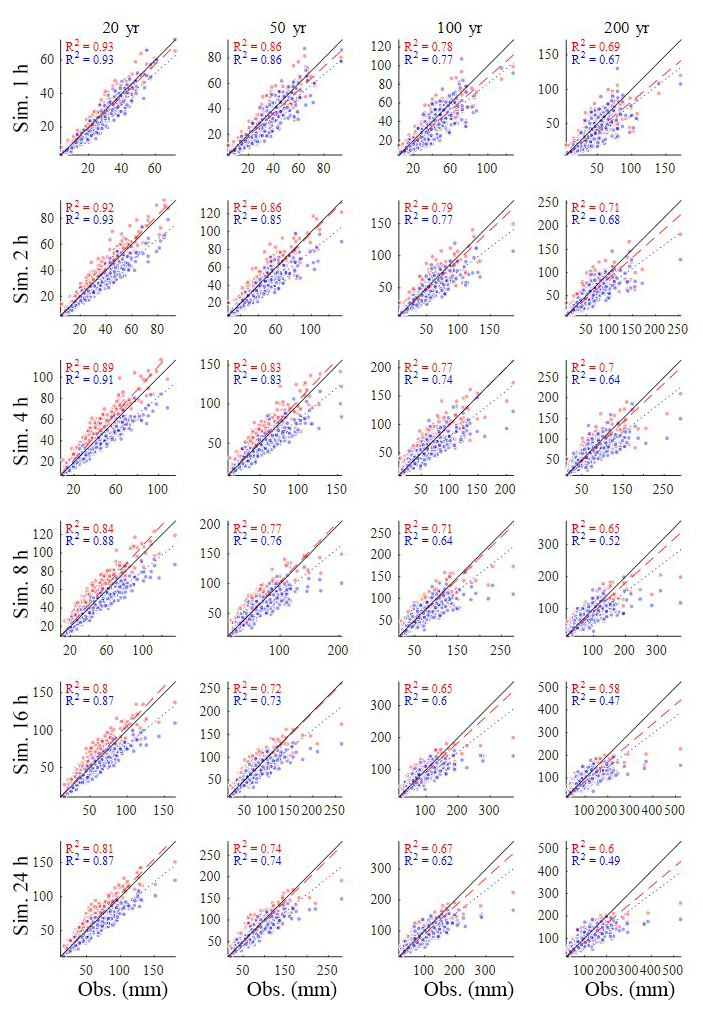
Figure 13 Comparison of the extreme rainfall values estimated from the observed rainfall (x) and synthetic rainfall (y) generated by the model of this study (red) and the MBLRP model (blue). The plots compare 20, 50, 100, and 200 year rainfall at hourly to daily aggregation levels.

Figure 14 shows the degree of bias of extreme-value reproduction (slope of the regression line in Fig. 13) varying with the recurrence interval. The values corresponding to the traditional MBLRP model are also shown. The degree of underestimation of the traditional methods varies between 73 % and 87 %, and it tends to increase as the recurrence interval increases. A similar tendency was observed for our model, but the degree of underestimation was significantly reduced. For our model, the degree of underestimation is the greatest for the 1 h extreme rainfall and tends to decrease as the duration of the rainfall increases. This tendency was not observed with the traditional MBLRP model.

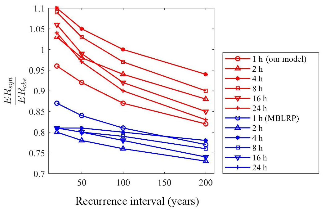
Figure 14 Degree of over- or underestimation of extreme values by our model (red) and the traditional MBLRP model (blue). ER_syn and ER_obs are extreme rainfall values estimated from synthetic rainfall and observed rainfall, respectively.

A good rainfall model should reproduce not only the extreme values but also the distribution of the maxima from which extreme values are derived. We performed the two-sample Kolmogorov–Smirnov (K-S) test between the monthly maxima of the synthetic rainfall and the observed rainfall. A significance level of 5 % was used. Among all 408 calendar months (34 gauges ×12 months), the null hypothesis of assuming that two distributions are the same could not be rejected at 384, 368, 317, 301, 323, and 333 months for the 1, 2, 4, 8, 16, and 24 h rainfall, respectively (83 % of all gauges). On the contrary, the traditional approach successfully reproduced the observed monthly maxima distribution only at 292, 243, 219, 200, 220, and 219 months (57 % of all gauges).

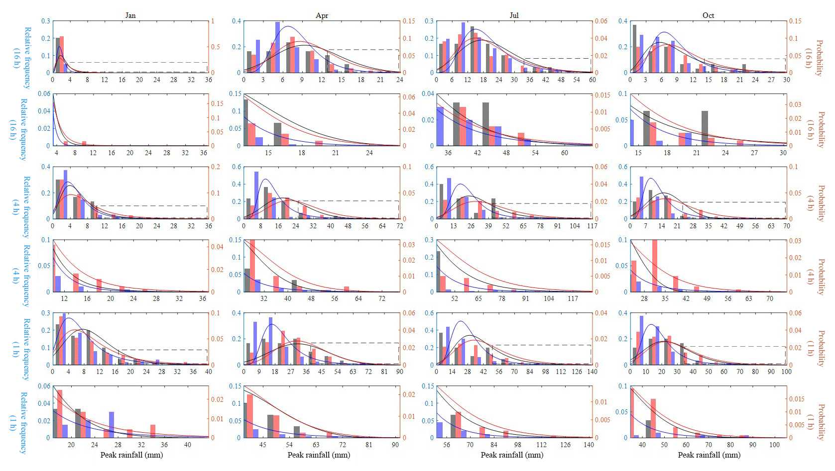
Figure 15 Relative frequency and the fitted GEV distribution of the 1, 4, and 16 h monthly maxima of January, April, July, and October rainfall at NCDC gauge 132203. Results of observed rainfall (black), our hybrid model (red), and the traditional MBLRP model (blue) are shown. The upper 10th percentile of the distribution (dashed box in the plots in the first, third, and fifth row) is magnified in the lower rows (plots in the second, fourth, and sixth row).

Figure 16 Comparison of the shape (ξ), scale (σ), and location (μ) parameters of the fitted GEV distribution of the monthly maxima. The results based on the observed rainfall (x), our hybrid model (red), and the traditional model (blue) are shown. The results of 1, 4, and 16 h rainfall durations are shown.

Figure 15 shows the relative frequency and the fitted GEV distribution of the monthly maxima of January, April, July, and October at NCDC gauge 132203. The black, red, and blue lines correspond to the result of observed rainfall, our hybrid model, and the traditional MBLRP model, respectively. The GEV distribution of the 1, 4, and 16 h rainfall durations are shown in the plots of the first, third, and fifth row, respectively. The plots in the second, fourth, and the sixth row magnify the upper 10th percentile of the distribution of the upper figures that is denoted as the dashed box. For all months and durations, our hybrid model outperforms the traditional MBLRP model in reproducing the head-to-tail part of the distribution. The distribution of the traditional MBLRP model was skewed toward the lower values. A similar tendency was observed at most gauge locations while at some of the gauges our hybrid model showed similar or slightly degraded performance compared to the traditional MBLRP model in reproducing the distribution of extreme values. We discuss this finding further in Sect. 5.1.

Figure 16 compares the shape (ξ), the scale (σ), and the location (μ) parameter of the fitted GEV distribution of the monthly maxima of the observed rainfall (x) and of the synthetic rainfall generated from our hybrid model (red scatters) and from the traditional MBLRP model (blue scatters). The results for 1, 4, and 16 h rainfall durations are shown. Each scatter point represents the result of one calendar month at one gauge. A total of 408 scatter points (12 months gauge⁻¹ × 34 gauges) are shown for each of the plots. The traditional MBLRP model underestimates the location parameters at all rainfall durations, and the degree of underestimation increases with increased duration. Our hybrid model showed the opposite trend. The location parameters tend to be overestimated with an increase in the duration, but the degree of overestimation was not as significant as in the case of the traditional model. The traditional model compensates for the underestimated location of the distribution with the overestimated scale parameters, which were observed for all three durations investigated. Our hybrid model also compensates for the overestimated location of the distribution with the underestimated scale parameters, but the degree of compensation was not as significant as in the case of the traditional model. However, the shape parameter of the observed monthly maxima was not well reproduced by either model. This result shows the difficulty of precisely reproducing the rainfall extreme values. This is mainly because the rainfall extreme values are indeed extreme. For example, a 1 h 100-year rainfall value corresponding to a 100-year rainfall record is theoretically the greatest value of all 72 000 hourly rainfall records (24 h day${}^{-\mathrm{1}}\times \mathrm{30}$ days month${}^{-\mathrm{1}}\times \mathrm{100}$ years), and precisely reproducing a value with such a low probability of occurrence can be a daunting task using the models with only a limited number of parameters.

5 Discussion

5.1 Variability of the parameters of the MBLRP model and extreme values

Our model uses different parameter sets of the MBLRP model to disaggregate different monthly rainfall values. This means that one given calendar month can have many different parameter sets. By contrast, the traditional MBLRP model uses one parameter set for each calendar month. Therefore, if we look at the variability of each month's parameters, we can see how the model of this study explains the variability of rainfall unlike the MBLRP model. Figure 17 shows a box plot of the parameters for each month at gauge NCDC-460582. The parameters of the traditional MBLRP model are shown together for reference (triangles). While significant variability is observed for all six parameters, the parameter μ, which represents the average rain cell intensity, showed the greatest variability, ranging over 2 orders of magnitude. This explains why our model is good at reproducing both large-scale rainfall variability and small-scale extreme values: the variability of the rain cell intensity parameter has the effect of stretching out the distribution of rainfall depths at a range of levels of aggregation, thereby increasing the probability of very large values. And the variability of this cell intensity parameter is also the most important factor responsible for the increase in the large-scale rainfall variance. Dimitriadis and Koutsoyiannis (2018) performed a similar experiment where a given degree of stochasticity was introduced to the parameter representing the rainfall mean, which subsequently influenced the higher-order moments at large timescales. In addition, Zorzetto et al. (2016) briefly discussed this matter. They introduced a novel framework of meta-statistical extreme-value (MEV) analysis. In this MEV formulation, one can show that interannual variation of exponential-type rainfall processes leads to a fat tail for its extreme values.

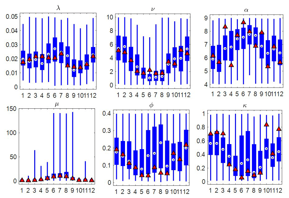
Figure 17 Variability of the six parameters of the MBLRP model of this study (box plot) at gauge NCDC-460582 (star mark in Fig. 3). The parameters of the traditional MBLRP model are shown together for reference (triangle).

The physical characteristics of rainfall can be estimated using Eqs. (11) and (12) to (15). We repeated the same analysis on these variables to compare the variability of the rainfall characteristics of our hybrid mode and that of the MBLRP model.

$$\begin{array}{}\text{(12)}& {\displaystyle }& {\displaystyle }\mathrm{Average}\mathrm{rainfall}\mathrm{depth}\mathrm{per}\mathrm{storm}\left(\mathrm{mm}\right)=\left(\mathrm{1}+{\displaystyle \frac{\mathit{\kappa }}{\mathit{\varphi }}}\right)\left({\displaystyle \frac{\mathit{\nu }}{\mathit{\alpha }}}\right)\mathit{\mu }\text{(13)}& {\displaystyle }& {\displaystyle }\mathrm{Average}\mathrm{number}\mathrm{of}\mathrm{rain}\mathrm{cells}\mathrm{per}\mathrm{storm}=\mathrm{1}+{\displaystyle \frac{\mathit{\kappa }}{\mathit{\varphi }}}\text{(14)}& {\displaystyle }& {\displaystyle }\mathrm{Average}\mathrm{rain}\mathrm{cell}\mathrm{arrival}\mathrm{rate}\left(h^{-\mathrm{1}}\right)=\mathit{\kappa }{\displaystyle \frac{\mathit{\alpha }}{\mathit{\upsilon }}}\text{(15)}& {\displaystyle }& {\displaystyle }\mathrm{Average}\mathrm{rain}\mathrm{cell}\mathrm{duration}\left(\mathrm{h}\right)={\displaystyle \frac{\mathit{\nu }}{\mathit{\alpha }}}\end{array}$$

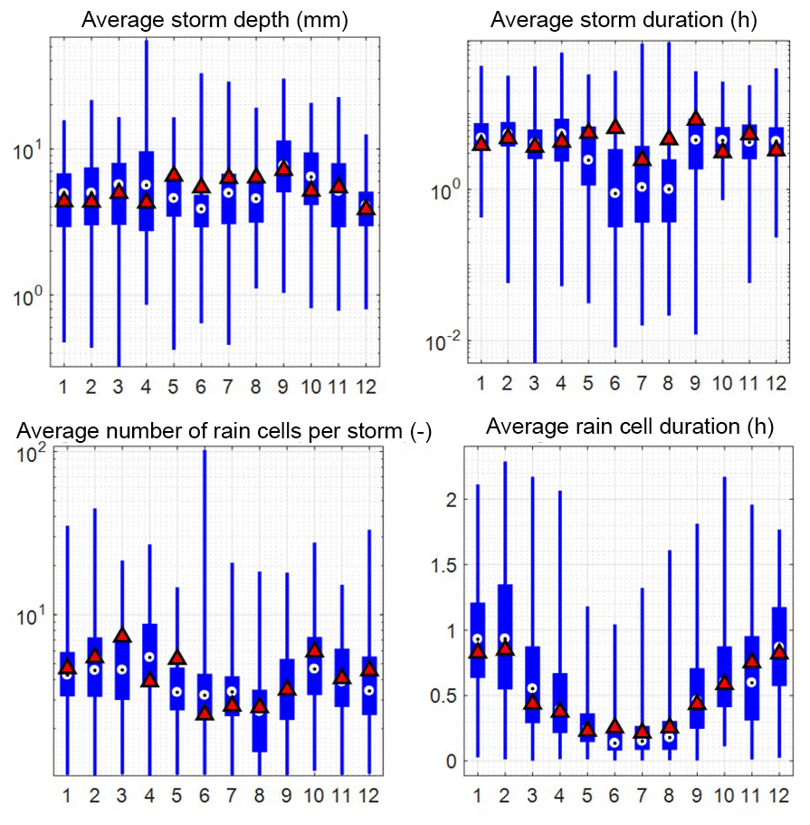
Figure 18 Variability of the rainfall characteristics of the MBLRP model of this study (box plot) at gauge NCDC-460582 (star mark in Fig. 3). The rainfall characteristics of the traditional MBLRP model are shown together for reference (triangle).

Figure 18 shows box plots of the various rainfall characteristics for each month at gauge NCDC-460582. The values were calculated using Eqs. (11) to (15). The rainfall characteristics of the traditional MBLRP model are shown together for reference (triangles). The variability of the average storm depth, the average storm duration, and the average number of rain cells per storm was significant, so the y axes of the box plots were drawn in log scale. This result suggests that the parameter variability that is incorporated in our model's distinct algorithm contributes to the highly variable external (average storm depth, average storm duration) and internal (average number of rain cells per storm, average rain cell duration) properties of the generated rainfall.

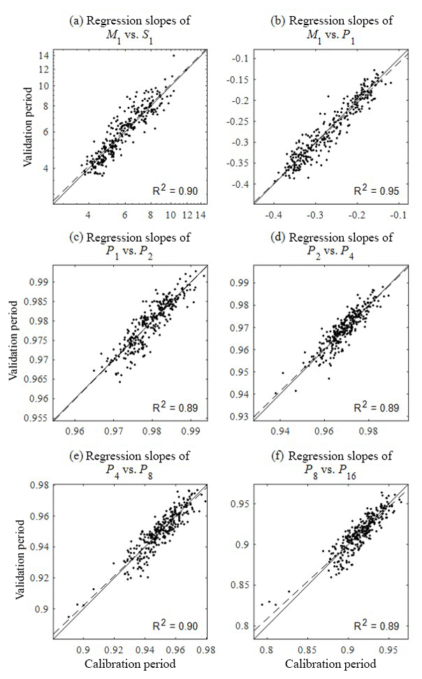
Figure 19 Comparison of the slope of regression analysis between the statistics shown in Fig. 6 for the calibration (x) and validation (y) period. The slopes of regression analysis (a) between the mean and standard deviation, (b) between the mean and proportion of dry periods, and (c–f) between the proportion of dry periods at the different timescales were compared. Solid lines are 1:1 line and dashed lines represent the regression lines.

5.2 An issue with model parsimoniousness: 6 versus 55

Our hybrid model uses 1 MBLRP model parameter set per 1 simulation month of 1 year while the MBLRP model needs only 6 parameters regardless of the simulation length. However, this does not mean that our model requires 600 MBLRP model parameters (6 per month ×100 months) to generate 100 months of rainfall. This is because parameters are estimated based on the sub-daily-scale rainfall statistics that are synthetically generated through the process of the SARIMA model and the regression analysis (see Fig. 5). Therefore, the parameters of the SARIMA model and the parameters of the regression analyses shown in Fig. 5 should be considered as the “true” parameters of this model because once these parameters are given, our model can generate infinite lengths of rainfall records. The SARIMA model has 6 parameters, and a set of regression analysis shown in Fig. 5 has 49 parameters (2 for each of 10 solid arrows in Fig. 5 equals 20, 3 per 8 bivariate normal distributions relating two subsequent residual terms (ε_i) in Fig. 5 equals 24, and one for each of 5 normal distributions perturbing autocorrelation terms (c_i) equals 5). Therefore, our model has a total of 55 parameters. This discrepancy in the number of parameters (6 for the traditional of MBLRP model versus 55 of our hybrid model) can be considered as a cost taken to reproduce the large-scale rainfall variability that the traditional MBLRP model cannot.

We admit that this large discrepancy of model parsimoniousness is an issue to be resolved for our model to be applied in practice. Regarding this, we are planning to apply our model to additional gauge locations across the world and share the result through the website (http://www.letitrain.info, last access: 15 February 2019). The work has been already initiated for the rainfall data of the Korean Peninsula.

5.3 Calibration versus validation

Our approach of separating the period of calibration and validation adopted to some gauge locations may seem surprising because most stochastic rainfall generators are calibrated based upon the statistics under an assumption of temporal stationarity of the rainfall process. According to this assumption, the statistics of the periods of calibration and the validation should be the same, which obviates the need for validating the model for separate periods. However, this assumption often does not account for cases in which, for example, the observation period is too short (e.g. a few extreme events are included in only one part of the time period) or the time series is indeed non-stationary. For this reason, the discrepancy of the model performance between the calibration and the validation period should not only be attributed to the model's limitations but also to the difference between statistics from the two periods. In view of these considerations, our primary purpose of separating the period of calibration and validation should be understood as an assessment of the model's applicability to rainfall generation for a future period. From the point of view of the calibration period, the validation period is an ungauged period just as any future period, and our model can be easily extended to the future period by adding a term accounting for long-term rainfall non-stationarity to the SARIMA model (first module). Our hybrid model assumes not only the stationarity of the typical rainfall statistics such as mean, variance, covariance and proportion of dry periods but also the relationship between them (see Fig. 6). The latter has not been explicitly discussed by previous studies, so it was also interesting to see whether such relationships between the statistics hold over different temporal periods and how the discrepancy affects the final model performance, if there is any. Figure 19 compares the slope of the regression analysis between the statistics shown in Fig. 6 for the calibration (x axis) and validation (y axis) periods. The plots corresponding to the variances at different scales are not shown because there are theoretical reasons for having a solid slope close to 2 (see Eq. 5 and the preceding equations). There is no a significant discrepancy between slopes estimated using statistics on calibration and validation periods, implying that relationships between the fine-timescale statistics are stationary and that our model can be used for future or ungauged periods.

6 Conclusions

The phenomena observed in hydrologic systems and the subsequent effects on human and environmental systems are the consequences of the complex interactions between the components that are influenced by rainfall variability at various ranges of timescales. Therefore, a good or realistic rainfall model must properly reflect the rainfall variability at all hydrologically relevant timescales. Its importance will gather more attention because of the recent trend in the hydrologic societies of recognizing the hydrologic, human, and environmental systems from a holistic view point and interpreting them based on continuous and dynamic simulations as opposed to the event-based simulations (Wagener et al., 2010).

This study is one of many recent efforts in this regard (Fatichi et al., 2011; Kim et al., 2013a; Paschalis et al., 2014). First, we showed that the Poisson cluster rainfall model, which is probably the most widely applied stochastic rainfall models cannot reproduce large-scale rainfall variability due to in-built limitations that lie in the model assumptions. Then, we showed that a combination of an autoregressive model for monthly timescales and the “well-tuned” Poisson cluster rainfall model for the finer ranges of timescales is capable of reproducing not only the first- to the third-order statistics of the rainfall depths, but also the intermittency properties of the observed rainfall.

An additional model could be integrated to our hybrid model to incorporate further rainfall variability, for example, an approach based on random cascades (Lombardo et al., 2012, 2017; Molnar and Burlando, 2005; Müller and Haberlandt, 2016; Pohle et al., 2018) can be integrated to our model to reproduce the rainfall variability at timescales as fine as 5 min; a multivariate downscaling approach (Koutsoyiannis et al., 2003; Moon et al., 2016) may be applied to obtain spatially consistent rainfall at multiple sites. In addition, the SARIMA model that was adopted in this study could be further modified to account for the coarser rainfall variability caused by the El Niño–Southern Oscillation (ENSO) and North Atlantic Oscillation (NAO). Lastly, the genuine structure of our model that is composed of a large-scale rainfall generation module and a downscaling module may be integrated to existing space–time rainfall generators to enhance their ability to generate large-temporal-scale rainfall variability (Burton et al., 2008; Müller and Haberlandt, 2015; Paschalis et al., 2013; Peleg and Morin, 2014; Peleg et al., 2017; Benoit et al., 2018).