Potential evaporation at eddy-covariance sites across the globe

Potential evaporation (E_p) is a crucial variable for hydrological forecasting and drought monitoring. However, multiple interpretations of E_p exist, which reflect a diverse range of methods to calculate it. A comparison of the performance of these methods against field observations in different global ecosystems is urgently needed. In this study, potential evaporation was defined as the rate of terrestrial evaporation (or evapotranspiration) that the actual ecosystem would attain if it were to evaporate at maximal rate for the given atmospheric conditions. We use eddy-covariance measurements from the FLUXNET2015 database, covering 11 different biomes, to parameterise and inter-compare the most widely used E_p methods and to uncover their relative performance. For each of the 107 sites, we isolate days for which ecosystems can be considered unstressed, based on both an energy balance and a soil water content approach. Evaporation measurements during these days are used as reference to calibrate and validate the different methods to estimate E_p. Our results indicate that a simple radiation-driven method, calibrated per biome, consistently performs best against in situ measurements (mean correlation of 0.93; unbiased RMSE of 0.56 mm day⁻¹; and bias of −0.02 mm day⁻¹). A Priestley and Taylor method, calibrated per biome, performed just slightly worse, yet substantially and consistently better than more complex Penman-based, Penman–Monteith-based or temperature-driven approaches. We show that the poor performance of Penman–Monteith-based approaches largely relates to the fact that the unstressed stomatal conductance cannot be assumed to be constant in time at the ecosystem scale. On the contrary, the biome-specific parameters required by simpler radiation-driven methods are relatively constant in time and per biome type. This makes these methods a robust way to estimate E_p and a suitable tool to investigate the impact of water use and demand, drought severity and biome productivity.

1 Introduction

Since its introduction 70 years ago by Thornthwaite (1948), the concept of potential evaporation (E_p), defined as the amount of water which would evaporate from a surface unconstrained by water availability, has been widely used in multiple fields. It has been incorporated in hydrological models dedicated to estimate runoff (e.g. Schellekens et al., 2017) or actual evaporation (Wang and Dickinson, 2012), as well as in drought severity indices (Sheffield et al., 2012; Vicente-Serrano et al., 2013). Long-term changes in E_p have been regarded as a driver of ecosystem distribution and aridity (Scheff and Frierson, 2013) and used to diagnose the influence of climate change on ecosystems based on climate model projections (e.g. Milly and Dunne, 2016). However, many different definitions of E_p exist, and consequently many different methods are available to calculate it. In recent years, there has been an increasing awareness of the impact of the underlying assumptions and caveats in traditional E_p formulations (Weiß and Menzel, 2008; Kingston et al., 2009; Sheffield et al., 2012; Seiller and Anctil, 2016; Bai et al., 2016; Milly and Dunne, 2016; Guo et al., 2017). As such, a global appraisal of the most appropriate method for assessing E_p is urgently needed. Yet, current formulations reflect a disagreement on the mere meaning of this variable, which requires the definition of some form of reference system (Lhomme, 1997). E_p has been typically defined as the evaporation which would occur in given meteorological conditions if water was not limited, either (i) over open water (Shuttleworth, 1993); (ii) over a reference crop, usually a wet (Penman, 1963) or irrigated (Allen et al., 1998) short green grass completely shading the ground; or (iii) over the actual ecosystem transpiring under unstressed conditions (Brutsaert, 1982; Granger, 1989).

A second source of disagreement on the definition of E_p relates to the spatial extent of the reference system and the consideration (or not) of feedbacks from the reference system on the atmospheric conditions. Several authors found it convenient to define E_p taking an extensive area as a reference system, because this reduces the influence of advection and entrainment flows (Penman, 1963; Priestley and Taylor, 1972; Brutsaert, 1982; Shuttleworth, 1993). Such an idealised extensive and well-watered ecosystem evaporating at maximal rate for the given atmospheric conditions can be expected to raise air humidity until the vapour pressure deficit (VPD) tends to zero. In this case, evaporation is only driven by radiative forcing and no longer by aerodynamic forcing. Meanwhile, others have defended the use of reference systems that are infinitesimally small (Morton, 1983; Pettijohn and Salvucci, 2009; Gentine et al., 2011b), in order to avoid the feedback of the reference system on aerodynamic forcing. The effect of the choice of reference system is best exemplified by the complementary relationship framework (Bouchet, 1964), which uses both approaches to link potential and actual evaporation, through $(\mathrm{1}+b)E_{{\mathrm{p}}_{\mathrm{0}}}=E_{\mathrm{pa}}+b{E}_{\mathrm{a}}$, with b an empirical constant (Kahler and Brutsaert, 2006; Aminzadeh et al., 2016), $E_{{\mathrm{p}}_{\mathrm{0}}}$ the evaporation from an extensive well-watered surface (i.e. in which the feedback from the ecosystem on the VPD and aerodynamic forcing is considered and where evaporation is only driven by a radiative forcing), E_pa the evaporation from a well-watered but infinitesimally small surface (i.e. where evaporation is driven by both radiative and aerodynamic forcing) and E_a the actual evaporation (Morton, 1983).

In light of all this controversy, the net radiation of the reference system remains another point of discussion: some scientists argue that the (well-watered) reference system should have the same net radiation as the actual (water-limited) system (e.g. Granger, 1989; Rind et al., 1990; Crago and Crowley, 2005). Yet, this is inherently inconsistent as the surface temperature reflects the surface energy partitioning; thus a well-watered system transpiring at a potential rate is expected to have a lower surface temperature (Maes and Steppe, 2012) and correspondingly a higher net radiation (e.g. Lhomme, 1997; Lhomme and Guilioni, 2006). Meanwhile, to some extent, the albedo also depends on soil moisture (Eltahir, 1998; Roerink et al., 2000; Teuling and Seneviratne, 2008) and it can be argued that it should be adjusted to reflect well-watered conditions (Shuttleworth, 1993). Finally, extensive reference surfaces can be expected to exert a feedback, not only on the aerodynamic forcing, but also on the incoming radiation (via impacts on air temperature, humidity and cloud formation). Yet, these larger-scale feedbacks are not acknowledged when computing E_p, even when considering extensive reference systems.

As it can be concluded from the above discussion, a unique and universally accepted definition of E_p does not exist, and the most appropriate definition remains tied to the specific interest and application. Nonetheless, as different applications make use of different E_p formulations, a good understanding of the implications of the choice for a specific method is required (Fisher et al., 2011). For terrestrial ecosystems, the use of an open-water reference system is uninformative about the actual available energy and the aerodynamic properties of the actual ecosystem (Shuttleworth, 1993; Lhomme, 1997). The approach of considering an idealised well-watered crop system only takes climate forcing conditions into account and not the actual land cover; as such, it has become the standard to estimate aridity and trends in global drought (Dai, 2011). When the actual ecosystem transpiring at unstressed rates is considered as a reference system, both climate forcing conditions and ecosystem properties are taken into account. This has been the preferred approach when calculating E_p as an intermediate step to estimate actual evaporation, often by applying a multiplicative stress factor (S) varying between 0 and 1, such that E_a=SE_p (e.g. Barton, 1979; Mu et al., 2007; Fisher et al., 2008; Miralles et al., 2011; Martens et al., 2017). This S factor can be considered analogous to the β factor used in some land surface models to incorporate the effect of soil moisture in the estimation of gross primary production and surface turbulent fluxes (Powell et al., 2013).

Several studies have attempted to compare and evaluate different E_p methods. Some of these studies have compared the performance of different E_p formulations in hydrological (Xu and Singh, 2002; Oudin et al., 2005a; Kay and Davies, 2008; Seiller and Anctil, 2016) or climate models (Weiß and Menzel, 2008; Lofgren et al., 2011; Milly and Dunne, 2016). Others considered the Penman–Monteith method as the benchmark to test less input-demanding formulations (e.g. Chen et al., 2005; Sentelhas et al., 2010). All these studies have their own merits, yet an evaluation of E_p methods based on empirical data of actual evaporation measurements is to be preferred (Lhomme, 1997). To date, such approaches have been hampered by limited data availability (Weiß and Menzel, 2008). Lysimeters provide arguably the most precise evaporation measurements available (e.g. Abtew, 1996; Pereira and Pruitt, 2004; Yoder et al., 2005; Katerji and Rana, 2011), but are sparsely distributed and not always representative of larger ecosystems. Pan evaporation measurements are more easy to perform and are broadly available (Zhou et al., 2006; Donohue et al., 2010; McVicar et al., 2012) but provide a proxy of open-water evaporation, rather than actual ecosystem potential evaporation; they also exhibit biases related to the location, shape and composition of the instrument (Pettijohn and Salvucci, 2009). Eddy-covariance measurements are an attractive alternative, but, apart from an unpublished study by Palmer et al. (2012), have so far only been used in E_p studies focusing on local to regional scales (Jacobs et al., 2004; Sumner and Jacobs, 2005; Douglas et al., 2009; Li et al., 2016).

The overall purpose of the present work is to identify the most suitable method to estimate E_p at the ecosystem-scale across the globe. Because we are using an empirical dataset of actual evaporation at FLUXNET sites, the reference system considered in this study is the actual ecosystem, so E_p is defined as the evaporation of the actual ecosystem when it is completely unstressed. As mentioned above, this definition is the most suitable for hydrological studies, studies of ecosystem drought and derivations of actual evaporation through constraining E_p calculations. Following this definition, E_p is similar to $E_{{\mathrm{p}}_{\mathrm{0}}}$ in the complementary relationship. We used the most recent and complete eddy-covariance database available, i.e. the FLUXNET2015 archive (http://fluxnet.fluxdata.org/, last access: 14 February 2019). The most frequently adopted E_p methods are applied based on standard parameterisations as well as calibrated parameters by biome and are inter-compared in order to gain insights into the most adequate means to estimate E_p from ecosystem to global scales.

2 Material and methods

2.1 Selection of E_p methods

Methods to calculate E_p can be categorised based on the amount and type of input data required. In this overview, we will only discuss the ones evaluated in our study, which are arguably the most frequently used.

2.1.1 Methods based on radiation, temperature, wind speed and vapour pressure

The well-known Penman–Monteith equation (Monteith, 1965) expresses latent heat flux λE_a (W m⁻²) as

$$\begin{array}{}\text{(1)}& {\displaystyle }{\displaystyle }\mathit{\lambda }{E}_{\mathrm{a}}={\displaystyle \frac{s\left(R_{\mathrm{n}}-G\right)+\frac{{\mathit{\rho }}_{\mathrm{a}}{c}_p\mathrm{VPD}}{r_{\mathrm{aH}}}}{s+\mathit{\gamma }+\mathit{\gamma }\frac{r_{\mathrm{c}}}{r_{\mathrm{aH}}}}},\end{array}$$

with λ being the latent heat of vaporisation (J kg⁻¹), E_a the actual evaporation (kg m⁻² s⁻¹), s the slope of the Clausius–Clapeyron curve relating air temperature with the saturation vapour pressure (Pa K⁻¹), R_n the net radiation (W m⁻²), G the ground heat flux (W m⁻²), ρ_a the air density (kg m⁻³), γ the psychrometric constant (Pa K⁻¹), c_p the specific heat capacity of the air (J kg⁻¹ K⁻¹), VPD the vapour pressure deficit (Pa), r_aH the resistance of heat transfer to air (s m⁻¹) and r_c the surface resistance of water transfer (s m⁻¹). While λ, c_p, s and γ are air-temperature-dependent, r_aH is a complex function of wind speed, vegetation characteristics and the stability of the lower atmosphere (see Sect. 2.3). In most methods to estimate E_a or E_p, r_aH is estimated from a simple function of wind speed.

The Penman–Monteith equation is frequently used to calculate E_p by adjusting r_c to its minimum value (the value under unstressed conditions). If the reference system is the actual system or a reference crop, r_c is usually considered a fixed, constant value larger than zero (even if the soil is well-watered). In this study, both a universal, fixed value of r_c for reference crops and a biome-specific constant value are used (see Sect. 2.5). When instead of a well-watered canopy a wet canopy (i.e. a canopy covered by water) is considered, r_c=0 and Eq. (1) collapses to

$$\begin{array}{}\text{(2)}& {\displaystyle }{\displaystyle }\mathit{\lambda }{E}_{\mathrm{p}}={\displaystyle \frac{s\left(R_{\mathrm{n}}-G\right)+\frac{{\mathit{\rho }}_{\mathrm{a}}{c}_p\mathrm{VPD}}{r_{\mathrm{aH}}}}{s+\mathit{\gamma }}}.\end{array}$$

Equation (2) is often referred to as the Penman (1948) formulation and can be conveniently rearranged as $\mathit{\lambda }{E}_{\mathrm{p}}=\frac{s(R_{\mathrm{n}}-G)}{s+\mathit{\gamma }}+\frac{{\mathit{\rho }}_{\mathrm{a}}{c}_p\mathrm{VPD}}{(s+\mathit{\gamma })r_{\mathrm{aH}}}$ to illustrate that E_p is driven by a radiative (left term) and an aerodynamic (right term) forcing (Brutsaert and Stricker, 1979).

2.1.2 Methods based on radiation and temperature

When the reference system is considered an idealised extensive area, or when radiative forcing is very dominant, the aerodynamic component of Eq. (2) may become negligible; thus the whole equation collapses to $\mathit{\lambda }{E}_{\mathrm{p}}=\frac{s(R_{\mathrm{n}}-G)}{s+\mathit{\gamma }}$, which is commonly referred to as “equilibrium evaporation” (Slatyer and McIlroy, 1961). Priestley and Taylor (1972) analysed time series of open water and water-saturated crops and grasslands and found that the evaporation over these surfaces closely matched the equilibrium evaporation corrected by a multiplicative factor, commonly denoted as α_PT:

$$\begin{array}{}\text{(3)}& {\displaystyle }{\displaystyle }\mathit{\lambda }{E}_{\mathrm{p}}={\mathit{\alpha }}_{\mathrm{PT}}{\displaystyle \frac{s\left(R_{\mathrm{n}}-G\right)}{s+\mathit{\gamma }}}.\end{array}$$

This formulation is known as the Priestley and Taylor equation. Because usually a constant value of α_PT is adopted, it assumes that the aerodynamic term in the Penman equation (Eq. 2) is a constant fraction of the radiative term. Typically, α_PT=1.26 is considered, as estimated by Priestley and Taylor (1972) in their original experiments. In this study, we also include a biome-specific value to extend its applicability to all biomes (see Sect. 2.5). Since this method does not require wind speed or VPD as input, it is widely applied in hydrological models (Norman et al., 1995; Castellvi et al., 2001; Agam et al., 2010), remote sensing evaporation models (Norman et al., 1995; Fisher et al., 2008; Agam et al., 2010; Miralles et al., 2011) and drought monitoring methods (Anderson et al., 1997; Vicente-Serrano et al., 2018).

2.1.3 Methods based on radiation

Other studies such as Lofgren et al. (2011), or the more recent Milly and Dunne (2016), further simplified Eq. (3) to make it a linear function of the available energy by defining a constant multiplier here referred to as α_MD:

$$\begin{array}{}\text{(4)}& {\displaystyle }{\displaystyle }\mathit{\lambda }{E}_{\mathrm{p}}={\mathit{\alpha }}_{\mathrm{MD}}\left(R_{\mathrm{n}}-G\right).\end{array}$$

In the case of Milly and Dunne (2016) this equation was applied to climate model outputs based on a constant and universal value of α_MD=0.8. On a daily scale, (R_n−G) expresses the total amount of energy available for evaporation, and the fraction of this energy that is actually used for evaporation is typically referred to “evaporative fraction”, or $\mathrm{EF}=\frac{\mathit{\lambda }{E}_{\mathrm{a}}}{(H+\mathit{\lambda }{E}_{\mathrm{a}})}=\frac{\mathit{\lambda }{E}_{\mathrm{a}}}{(R_{\mathrm{n}}-G)}$. From Eq. (4), it follows that the parameter α_MD can be interpreted as the EF of the unstressed ecosystem. In this study, we test both the general value of α_MD=0.8 and a biome-specific constant (see Sect. 2.5).

2.1.4 Methods based on temperature

Of the many empirical methods to estimate E_p, temperature-based methods have arguably been the most commonly used because of the availability of reliable air temperature data. For an overview of these methods, we refer to Oudin et al. (2005a). In this study, three methods are included. First, Pereira and Pruitt (2004) formulated a daily version of the well-known Thornthwaite (1948) equation:

$$\begin{array}{}\text{(5a)}& {\displaystyle }& {\displaystyle }{T}_{\mathrm{eff}}<\mathrm{0}\mathit{\lambda }{E}_{\mathrm{p}}=\mathrm{0},\text{(5b)}& {\displaystyle }& {\displaystyle }\mathrm{0}<T_{\mathrm{eff}}<\mathrm{26}\mathit{\lambda }{E}_{\mathrm{p}}={\mathit{\alpha }}_{\mathrm{Th}}{\left({\displaystyle \frac{\mathrm{10}{T}_{\mathrm{eff}}}{I}}\right)}^b\left({\displaystyle \frac{N}{\mathrm{360}}}\right),\text{(5c)}& {\displaystyle }& {\displaystyle }\mathrm{26}<T_{\mathrm{eff}}\mathit{\lambda }{E}_{\mathrm{p}}=-c+d{T}_{\mathrm{eff}}-e{T}_{\mathrm{eff}}^{\mathrm{2}},\end{array}$$

with T_eff the effective temperature, based on maximum and minimal temperatures (see Sect. 2.5); α_Th an empirical parameter (see below); I the yearly sum of (T_{a_month}∕5)^1.514, with T_{a_month} the mean air temperature for each month; N the number of daylight hours; b a parameter depending on I and c; and d and e empirical constants (see Sect. 2.5). The general value of α_Th=16 is often adopted; in this study, we will also calculate and apply a biome-specific value.

The second temperature-based formulation is that proposed by Oudin et al. (2005a), selected and developed after comparing 27 physically based and empirical methods with runoff data from 308 catchments:

$$\begin{array}{}\text{(6a)}& {\displaystyle }& {\displaystyle }{T}_{\mathrm{a}}<\mathrm{5}\mathit{\lambda }{E}_{\mathrm{p}}=\mathrm{0},\text{(6b)}& {\displaystyle }& {\displaystyle }{T}_{\mathrm{a}}>\mathrm{5}\mathit{\lambda }{E}_{\mathrm{p}}={\displaystyle \frac{R_e}{{\mathit{\rho }}_{\mathrm{a}}}}{\displaystyle \frac{\left(T_{\mathrm{a}}-\mathrm{5}\right)}{{\mathit{\alpha }}_{\mathrm{Ou}}}},\end{array}$$

with T_a the air temperature (^∘C) and R_e the top-of-atmosphere radiation (MJ m⁻² day⁻¹), depending on latitude and Julian day. Oudin et al. (2005a) suggested the use of α_Ou=100. This value will be used, in addition to a biome-specific value.

Finally, the third temperature-based method is the Hargreaves and Samani (1985) formulation, which includes minimum (T_min) and maximum (T_max) daily temperature, next to T_a and R_e:

$$\begin{array}{}\text{(7)}& {\displaystyle }{\displaystyle }\mathit{\lambda }{E}_{\mathrm{p}}={\mathit{\alpha }}_{\mathrm{HS}}{R}_e\left(T_{\mathrm{a}}+\mathrm{17.8}\right)\sqrt{T_{\max }-T_{\min }},\end{array}$$

with α_HS a constant, normally assumed to equal 0.0023. As for the other methods, we additionally apply a biome-specific value. A detailed description of the calibration of all E_p methods is given in Sect. 2.5.

2.2 FLUXNET2015 database

The Tier 2 FLUXNET2015 database based on half-hourly or hourly measurements from eddy-covariance sensors is used to evaluate the different E_p formulations (http://fluxnet.fluxdata.org/data/fluxnet2015-dataset/, last access: 14 February 2019). Sites lacking at least one of the basic measurements required for our analysis (i.e. R_n; G; λE_a; H; precipitation; wind speed, u; friction velocity, u_*; T_a; and relative humidity, RH, or VPD) were not considered further. For latent and sensible heat fluxes, we used the data corrected by the Bowen ratio method. In this approach, the Bowen ratio is assumed to be correct, and the measured λE_a and H are multiplied by a correction factor derived from a moving window method; see http://fluxnet.fluxdata.org/data/fluxnet2015-dataset/data-processing/ (last access: 14 February 2019) for a detailed description of this standard procedure. Nonetheless, taking the uncorrected λE_a instead did not impact the main findings (not shown). For the main heat fluxes (G, H, λE_a), medium and poor gap-filled data were masked out according to the flags provided by FLUXNET. As no quality flag was available for R_n measurements, the flag of the shortwave incoming radiation was used instead. All negative values for H or λE_a were masked out, as these relate to periods of interception loss and condensation when accurate measurements are not guaranteed (Mizutani et al., 1997). Similarly, all negative values of R_n were masked out.

Finally, sub-daily measurements were aggregated to daytime composites (i) by applying a minimum threshold of 5 W m⁻² of top-of-atmosphere incoming shortwave radiation and (ii) after excluding the first and last (half-)hours from these aggregates. Based on these daytime aggregates, the daytime means of s, γ and ρ_a were calculated using the parameterisation procedure described by Allen et al. (1998). We used T_a to calculate s. Only days in which more than 70 % of the data were measured directly were retained, and days with rainfall (between midnight and sunset) were removed from the analyses to avoid the effects of rainfall interception. Furthermore, only sites with at least 80 retained days were used for the further analysis. The global distribution of the final selection of sites is shown in Fig. 1 and detailed information about these sites is provided in Table S1 of the Supplement. The IGBP classification was used to assign a biome to each site.

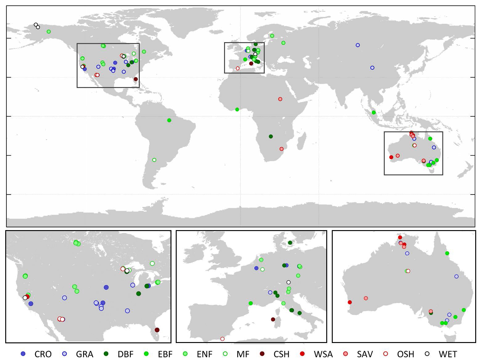
Figure 1 Location of the flux sites used in this study per biome. CRO: cropland; GRA: grasslands; DBF: deciduous broadleaf forest; EBF: evergreen broadleaf forest; ENF: evergreen needleleaf forest; MF: mixed forest; CSH: closed shrubland; WSA: woody savannah; SAV: savannah; OSH: open shrubland; WET: wetlands.

2.3 Calculation of resistance parameters

Estimates of r_aH are required for the Penman and Penman–Monteith equations. The resistance of heat transfer to air, r_aH, was calculated as

$$\begin{array}{ll}{\displaystyle }{r}_{\mathrm{aH}}& {\displaystyle }={\displaystyle \frac{u}{u_{*}^{\mathrm{2}}}}+{\displaystyle \frac{\mathrm{1}}{k{u}_{*}}}\left[\ln \left({\displaystyle \frac{z_{\mathrm{0}\mathrm{m}}}{z_{\mathrm{0}\mathrm{h}}}}\right)+{\mathrm{\Psi }}_{\mathrm{m}}\left({\displaystyle \frac{z-d}{L}}\right)-{\mathrm{\Psi }}_{\mathrm{m}}\left({\displaystyle \frac{z_{\mathrm{0}\mathrm{h}}}{L}}\right)\right.\\ \text{(8)}& {\displaystyle }& {\displaystyle }\left.-{\mathrm{\Psi }}_{\mathrm{h}}\left({\displaystyle \frac{z-d}{L}}\right)+{\mathrm{\Psi }}_{\mathrm{h}}\left({\displaystyle \frac{z_{\mathrm{0}\mathrm{h}}}{L}}\right)\right],\end{array}$$

in which k=0.41 is the von Kármán constant; z the (wind) sensor height (m); d the zero displacement height (m); z_0m and z_0h the roughness lengths for momentum and sensible heat transfer (m), respectively; L the Obukhov length (m); and Ψ_m(X) and Ψ_h(X) the Businger–Dyer stability functions for momentum and heat for the variable X, respectively. These were calculated based on the equations given by Garratt (1992) and Li et al. (2017) for stable, neutral and unstable conditions. Note that, in neutral and stable conditions, Ψ_m(X)=Ψ_h(X) and that ${\mathrm{\Psi }}_{\mathrm{m}}\left(\frac{z-d}{L}\right)-{\mathrm{\Psi }}_{\mathrm{m}}\left(\frac{z_{\mathrm{0}\mathrm{h}}}{L}\right)-{\mathrm{\Psi }}_{\mathrm{h}}\left(\frac{z-d}{L}\right)+{\mathrm{\Psi }}_{\mathrm{h}}\left(\frac{z_{\mathrm{0}\mathrm{h}}}{L}\right)=\mathrm{0}$. This is not the case for the unstable conditions that usually prevail during the daytime. Daytime averages of all variables were used as input in Eq. (8). The sensor height z was collected individually for each tower through online and literature research or through personal communication with the towers' principal investigator. The Obukhov length L was calculated as

$$\begin{array}{}\text{(9)}& {\displaystyle }{\displaystyle }L={\displaystyle \frac{-u_{*}^{\mathrm{3}}{\mathit{\rho }}_{\mathrm{a}}{T}_{\mathrm{a}}\left(\mathrm{1}+\mathrm{0.61}{q}_a\right)c_p}{kgH}},\end{array}$$

with q_a being the specific humidity (kg kg⁻¹) and g=9.81 m s⁻² the gravitational acceleration.

The displacement height d and the roughness length for momentum flux z_0m were estimated as a function of the canopy vegetation height (VH), as d=0.66 VH and z_0m=0.1 VH (Brutsaert, 1982). VH was estimated from the flux tower measurements using the approach of Pennypacker and Baldocchi (2016):

$$\begin{array}{}\text{(10)}& {\displaystyle }{\displaystyle }\mathrm{VH}={\displaystyle \frac{z}{\mathrm{0.66}+\mathrm{0.1}\exp \left(\frac{ku}{u_{*}}\right)}}.\end{array}$$

This equation was applied to the full (half-)hourly database and only when conditions were near-neutral ($|z/L|<\mathrm{0.01}$) and friction velocities lower than 1 standard deviation below the mean u_* at each site. The daily VH was then aggregated by averaging out the half-hourly estimates to daily values, excluding the 20 % outliers of the data, and then calculating a 30-day-window moving average on the dataset. When not enough (half-)hourly vegetation height observations (<160) were available, the site was excluded from the analysis. This gave robust results for all remaining sites; an example of VH temporal development for a specific location is given in Fig. 2a. For homogeneous canopies, the VH calculated this way represents the true vegetation height. For savannah-like ecosystems, it corresponds to the vegetation height that the vegetation would have if it was represented by a single big leaf model.

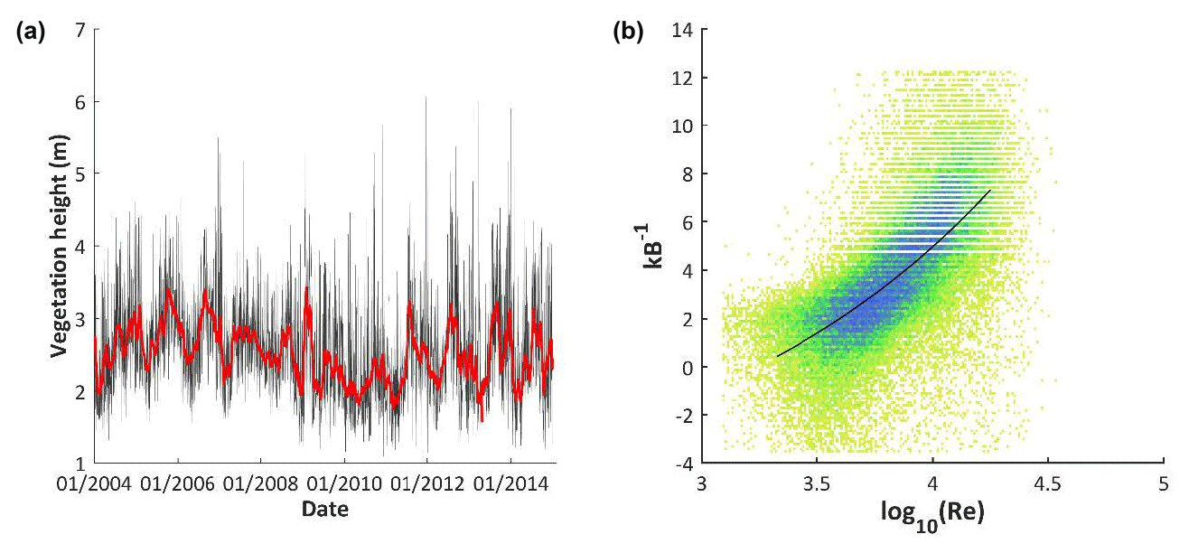
Figure 2 (a) Vegetation height dynamics in time (grey dots: half-hourly measurements; dark grey lines: daily mean vegetation height; red line: 30-day moving average, i.e. the final vegetation height dataset). (b) Relation between Stanton number (kB⁻¹) and Reynolds number (Re). Both plots correspond to the woody savannah site of Santa Rita Mesquite, US-SRM (Arizona, USA).

The Stanton number (defined as $k{B}^{-\mathrm{1}}=\ln \left(z_{\mathrm{0}\mathrm{m}}{z}_{\mathrm{0}\mathrm{h}}^{-\mathrm{1}}\right)$) was calculated by assuming that the surface aerodynamic temperature T₀ (defined by $H={\mathit{\rho }}_{\mathrm{a}}{c}_p\frac{(T_{\mathrm{0}}-T_{\mathrm{a}})}{r_{\mathrm{aH}}}$) is equal to the radiative surface temperature T_s derived from the longwave fluxes. Then, through an iterative approach, an optimal value of z_0h was obtained, using the following equations for T₀ (Garratt, 1992) and T_s (Maes and Steppe, 2012):

$$\begin{array}{ll}{\displaystyle }{T}_{\mathrm{0}}& {\displaystyle }=T_{\mathrm{a}}+\left({\displaystyle \frac{H}{k{u}_{*}{\mathit{\rho }}_{\mathrm{a}}{c}_p}}\right)\left[\ln \left({\displaystyle \frac{z-d}{z_{\mathrm{0}\mathrm{h}}}}\right)-{\mathrm{\Psi }}_{\mathrm{h}}\left({\displaystyle \frac{z-d}{L}}\right)\right.\\ \text{(11)}& {\displaystyle }& {\displaystyle }\left.+{\mathrm{\Psi }}_{\mathrm{h}}\left({\displaystyle \frac{z_{\mathrm{0}\mathrm{h}}}{L}}\right)\right],\end{array}$$

$$\begin{array}{}\text{(12)}& {\displaystyle }{\displaystyle }{T}_{\mathrm{s}}=\sqrt[\mathrm{4}]{{\displaystyle \frac{{\mathrm{LW}}_{\mathrm{out}}-(\mathrm{1}-\mathit{\epsilon }){\mathrm{LW}}_{\mathrm{in}}}{\mathit{\sigma }\mathit{\epsilon }}}},\end{array}$$

with σ the Stefan–Boltzmann constant and ε the emissivity. The (half-)hourly data were used for this calculation. Following the approach of Li et al. (2017), only summertime data were used, and only when H was larger than 20 W m⁻² and u_* larger than 0.01 m s⁻¹. Summertime was defined as those months in which the maximal daily value of H is at least 85 % of the 98th percentile of H based on the entire tower time series. In addition, (half-)hourly observations with counter-gradient heat fluxes were excluded from the analysis. For each observation, z_0h was optimised by minimising the difference between T₀ and T_s. Then, kB⁻¹ was calculated at each site based on its relation with the observed Reynolds number (Re) by fitting the following function, based on the work by Li et al. (2017):

$$\begin{array}{}\text{(13)}& {\displaystyle }{\displaystyle }k{B}^{-\mathrm{1}}=a_{\mathrm{0}}+a_{\mathrm{1}}R{e}^{a\mathrm{2}}.\end{array}$$

Note that Eq. (12) requires a value for ε, which is often assumed to be equal to 0.98 for all sites (e.g. Li et al., 2017; Rigden and Salvucci, 2015). Under the assumption that T₀=T_s, ε can also be calculated separately per site. If H=0, it follows that T₀=T_a and, from Eq. (12),

$$\begin{array}{}\text{(14)}& {\displaystyle }{\displaystyle }\mathit{\epsilon }={\displaystyle \frac{{\mathrm{LW}}_{\mathrm{out}}-{\mathrm{LW}}_{\mathrm{in}}}{\mathit{\sigma }{T}_{\mathrm{a}}^{\mathrm{4}}-{\mathrm{LW}}_{\mathrm{in}}}}.\end{array}$$

Here, ε was calculated for each site using (half-)hourly data, selecting those measurements where H was close to 0 ($-\mathrm{2}<H<\mathrm{2}$ W m⁻²) and excluding rainy days as well as measurements in which the albedo (calculated as α = SW_outSW${}_{\mathrm{in}}^{-\mathrm{1}}$ with SW_in the incoming and SW_out the outgoing shortwave radiation) was above 0.4, to avoid influences of snow or ice. Negative estimates of ε were masked out, and the ε of the site was calculated as the mean, after excluding the outlying 20 % of the data. Equation (3) was applied both with a fixed ε of 0.98 and with the observed ε, and the ε value yielding the lowest RMSE in Eq. (12) was retained for each site. An example of such a function between kB⁻¹ and Re is shown in Fig. 2b.

Finally, the surface resistance r_c (s m⁻¹) was calculated by inverting the Penman–Monteith equation as

$$\begin{array}{}\text{(15)}& {\displaystyle }{\displaystyle }{r}_{\mathrm{c}}={\displaystyle \frac{s\left(R_{\mathrm{n}}-G\right)r_{\mathrm{aH}}+{\mathit{\rho }}_{\mathrm{a}}{c}_p\mathrm{VPD}}{\mathit{\gamma }\mathit{\lambda }{E}_{\mathrm{a}}}}-{\displaystyle \frac{(s+\mathit{\gamma })r_{\mathrm{aH}}}{\mathit{\gamma }}}.\end{array}$$

We converted the r_c estimates to surface conductance g_c (mm s⁻¹) using $g_{\mathrm{c}}=\mathrm{1000}{r}_{\mathrm{c}}^{-\mathrm{1}}$; we will continue using g_c (rather than r_c) for the remainder of this paper. Note that the approach of calculating kB⁻¹ directly requires a separate measurement of LW_in and LW_out, which was only available in 95 of the 107 selected sites. For the remaining sites, an alternative approach was used to calculate kB⁻¹ (see Supplement).

2.4 Selection of unstressed days

We include two different approaches to identify a subset of measurements per eddy-covariance site in which the ecosystem was unstressed and provide the results for both methods. A first approach is based on soil moisture levels. For those sites where soil moisture measurements were available, the maximal soil moisture level for each site was determined as the 98th percentile of all soil moisture measurements. We then split up the dataset of each site in five equal-size classes based on evaporation percentiles. For each class, days having soil moisture levels belonging to the highest 5 % of soil moisture levels within each class were selected as unstressed days, but only if the soil moisture level of these selected days was above 75 % of the maximum soil moisture. This guaranties the sampling of unstressed evaporation during all seasons.

As soil moisture data were not available for a large number of sites, and because using soil moisture data does not exclude days in which evaporation may be constrained by other kinds of biotic or abiotic stress, a second approach for defining unstressed days was applied based on an energy balance criterion. We calculated the EF from the daytime λE_a and H values and considered it as a direct proxy for evaporative stress; i.e. we assumed that, under unstressed conditions, a larger fraction of the available energy is used to evaporate water (Gentine et al., 2007, 2011a; Maes et al., 2011). This approach is similar to those of other E_p studies using eddy-covariance or lysimeter data, in which the Bowen ratio (e.g. Douglas et al., 2009) or the ratio of λE_a and (SW_in + LW_in) (Pereira and Pruitt, 2004) are used to define unstressed days. The unstressed record was comprised of all days with EF exceeding the 95th percentile EF threshold for each particular site or, if fewer than 15 days fulfilled this criterion, the 15 days with the highest EF. Consequently, we assume that at each site during at least 5 % of the days the conditions are such that evaporation is unstressed and E_a reflects E_p. The measured E_a from the identified unstressed days is further referred to as E_unstr (mm day⁻¹) and used as reference data to evaluate the different E_p methods.

To assess whether the atmospheric conditions of the unstressed datasets are representative for the FLUXNET sites as such, a random bootstrap sample having the same number of records as the unstressed dataset was taken from the entire dataset of daily records. The mean, standard deviation, and 2nd and 98th percentile of SW_in, T_a, VPD and u were calculated. This procedure was repeated 1000 times per site. A t test comparing the values of the unstressed subsample with those of the 1000 random samples was used to analyse whether the atmospheric conditions of the unstressed subsample were representative for the overall site conditions. This analysis was carried out for both methods to select unstressed days: the soil moisture threshold and the energy balance criterion.

2.5 Calculation and calibration of the different E_p methods

An overview of the different methods to calculate E_p is given in Table 1. If possible, three versions of each method were calculated: (1) a reference crop version, (2) a standard version and (3) a biome-specific version. The reference crop version calculates E_p for the reference short turf grass crop, with R_n and other properties of this reference crop as well. The standard version uses the same non-biome-specific parameters of the reference crop but considers R_n and other properties of the actual ecosystem. The biome-specific version of each method applies a calibration of the key parameters per biome (Table 1) and considers R_n and other properties of the actual ecosystem. These calibrated values per biome are based on the mean value of this key parameter for the unstressed dataset for each site, averaged out per biome type.

Table 1 Overview of the different E_p methods used in this study and their calculation.

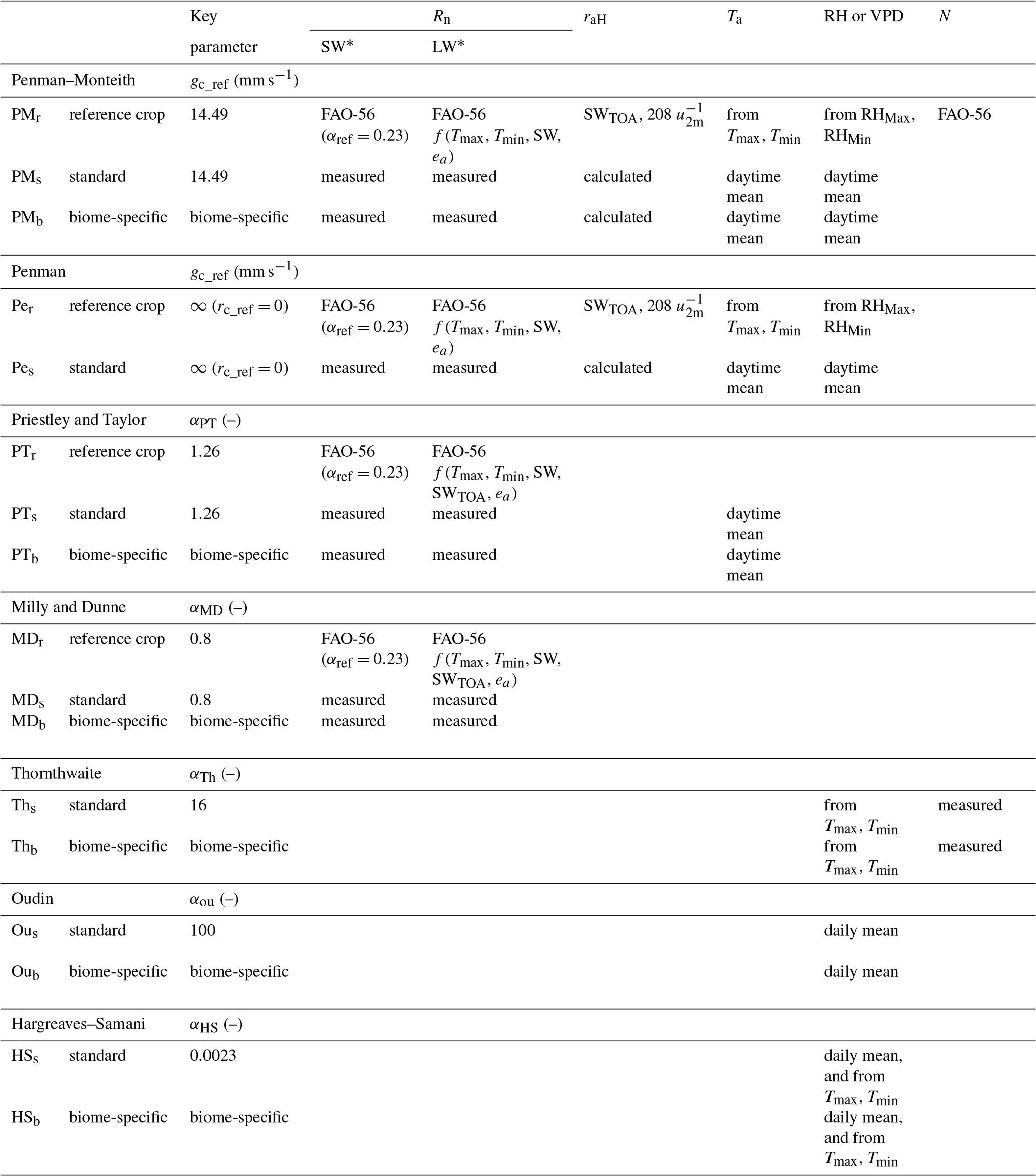
N is the number of daylight hours; T_max and T_min are the maximum and minimum daily air temperature; RH_max and RH_min are the maximum and minimum RH; SW^* and LW^* are the net shortwave and net longwave radiation; SW_TOA is the shortwave incoming radiation at the top of the atmosphere; FAO-56 refers to the methodology described by Allen et al. (1998).

To estimate the radiation and crop properties of the reference crop versions, the equations described by Allen et al. (1998) in the FAO-56 method (Food and Agricultural Organization) were used and G was considered to be 0. R_n was calculated as

$$\begin{array}{}\text{(16)}& {\displaystyle }{\displaystyle }{R}_{\mathrm{n}}={\mathrm{SW}}_{\mathrm{in}}\left(\mathrm{1}-{\mathit{\alpha }}_{\mathrm{ref}}\right)+{\mathrm{LW}}^{*},\end{array}$$

where α_ref=0.23 (Allen et al., 1998) and LW^* is the net longwave radiation, calculated after Allen et al. (1998; Eq. 39, Sect. 3).

In the case of the reference crop version of the Penman–Monteith equation (Eq. 1), the FAO-56 method was used as described by Allen et al. (1998), with g_{c_ref} fixed as 14.49 mm s⁻¹ (corresponding with r_{c_ref}=69 s m⁻¹) and using Eq. (16) to calculate R_n. The standard version of the Penman–Monteith equation used observed (R_n, G, VPD) and calculated (s, γ, ρ_a, r_aH) daytime values as described in Sect. 2.2 in Eq. (1), and it also assumed g_{c_ref}=14.49 mm s⁻¹. The biome-specific version was calculated with the same data but used a biome-dependent value of g_c. First, for each individual site, the unstressed g_c was calculated as the mean of the g_c values of the unstressed record (see Sect. 2.4). The mean value per biome was then calculated from these unstressed g_c values. Regarding the Penman method (Eq. 2), the reference crop and standard versions were calculated using the same input data as for the Penman–Monteith methods; given Penman's consideration of no surface resistance, no biome-specific version was calculated.

The reference crop version of the Priestley and Taylor method was calculated from Eq. (3) with R_n from Eq. (16), s and γ from the FAO-56 calculations, and with α_PT=1.26. The standard version used the same value for α_PT but the observed daytime values for R_n and G. The biome-specific version followed a calibration of α_PT similar to the g_{c_ref} calculation. For each site, the unstressed α_PT was calculated as the average α_PT, obtained by solving Eq. (3) for α_PT using the unstressed dataset. Finally, the mean per biome was calculated and used in the E_p estimation. Regarding the method by Milly and Dunne (2016) (Eq. 4), the reference crop, standard and biome-specific calculation were calculated accordingly, with R_n from Eq. (16) for the reference crop version, α_MD=0.8 for the reference crop and standard version, and a calibrated α_MD by biome type for the biome-specific version.

For the Thornthwaite, Oudin, and Hargreaves–Samani formulations (Eqs. 5–7), only the standard and biome-specific versions were calculated. The standard version of Thornthwaite's formulation used α_Th=16. In the biome-specific version, this parameter was again calculated per site as the mean value of the unstressed records (e.g. Xu and Singh, 2001; Bautista et al., 2009), and then averaged per biome type. The effective temperature T_eff was calculated as $T_{\mathrm{eff}}=\mathrm{0.36}(\mathrm{3}{T}_{\max }-T_{\min })$ (Camargo et al., 1999). The parameter b was calculated as $b=(\mathrm{6.75}\times {\mathrm{10}}^{-\mathrm{7}}{I}^{\mathrm{3}})(\mathrm{7.71}\times {\mathrm{10}}^{-\mathrm{7}}{I}^{\mathrm{2}})+\mathrm{0.0179}I+\mathrm{0.492}$ and the parameters c–e in Eq. (5c) were 415.85, 32.24 and 0.43, respectively (Pereira and Pruitt, 2004). For Oudin's temperature-based formulation, α_Ou=100 was taken for the standard version (Eq. 6). In the biome-specific version, this value was recalculated by calculating α_Ou for the unstressed records through Eq. (6), calculating the mean α_Ou per site and finally the biome-dependent α_Ou. Similarly, for the Hargreaves–Samani method, α_HS=0.0023 is used for the standard version (Eq. 7), whereas, in the biome-specific version, this value was calculated using the unstressed records. Altogether, this exercise yielded a total of 17 different methods to estimate E_p, whose specificities are documented in Table 1.

The influence of climatic forcing data on E_unstr and on g_{c_ref}, α_PT and α_MD was investigated. This was done by calculating for each individual site the correlations between the daily estimates of the atmospheric conditions and the daily values of the unstressed datasets. Analyses were then performed on these correlations of all sites.

3 Results

3.1 Representativeness of climate forcing data of unstressed datasets

Table S2 provides an overview of the analyses used to verify if the climatic forcing data of the unstressed subsets were representative for the atmospheric conditions of the sites as such. For the subsets of both unstressed criteria, atmospheric conditions were very representative for the site conditions, including for VPD. For the energy balance criterion, for instance, only at one site, the unstressed subset of the 98th percentile was significantly different from the random sampling-based simulations and in only two sites the 2nd percentile was significantly different from the simulations.

3.2 Key parameters by biome

We focus here on the parameter estimates of the unstressed record based on the energy balance criterion (Sect. 2.4). Of the full dataset, 107 flux sites meet all the selection criteria (i.e. at least 80 days without rainfall, good quality measurements of radiation and main fluxes, and at least 160 vegetation height observations – see Sect. 2.2 and 2.3). Despite considerable variation, g_{c_ref} does not differ statistically across biomes, in contrast with α_PT and α_MD. Overall, croplands (CRO) are characterised by a higher measured E_unstr, which translates into the highest g_{c_ref}, α_PT and α_MD of all biomes. Grasslands (GRA), deciduous broadleaf forest (DBF) and evergreen broadleaf forest (EBF) also have a relatively high g_{c_ref}, α_PT and α_MD, whereas mixed forest (MF) and savannah ecosystems (closed shrubland, CSH; woody savannah, WSA; open shrublands, OSH; and savannah, SAV, ecosystems) are characterised by lower g_{c_ref}, α_PT and α_MD. Only five sites (DE-Kli and IT-BCi, CRO; CA-SF3, OSH; AU-Rig, GRA; and AU-Wac, EBF) have mean values of α_PT higher than the typically assumed 1.26 (Table 2). In contrast, 27 sites, including 9 croplands, have a mean value of α_MD above 0.80, and 42 sites have a mean g_{c_ref} above 14.49 mm s⁻¹. Finally, wetlands (WET) show a large standard deviation of α_PT and α_MD (Table 2) due to their location in tropical, temperate and in arctic regions. The parameters of the three temperature-based methods differed significantly across biomes, but trends were different for each key parameter and did not always match those for g_{c_ref}, α_PT and α_MD (Table 2).

Table 2 Overview of the difference of the key parameters (g_{c_ref}, α_PT, α_MD, α_Th, α_Ou and α_HS) during unstressed conditions per biome. The energy balance method was used for defining unstressed days (see Sect. 2.4; see Table 1 for definition of key parameters). The p value of the ANOVA test is given, as well as the mean ±1 SD for each biome. Different alphabetic superscripts indicate significantly differing means (Tukey post-hoc test: p<0.05). The number of sites per biome is given between brackets. Different parts are used to group biomes into broader ecosystem types (in descending order: croplands, grasslands, forests, savannah ecosystems and wetlands).

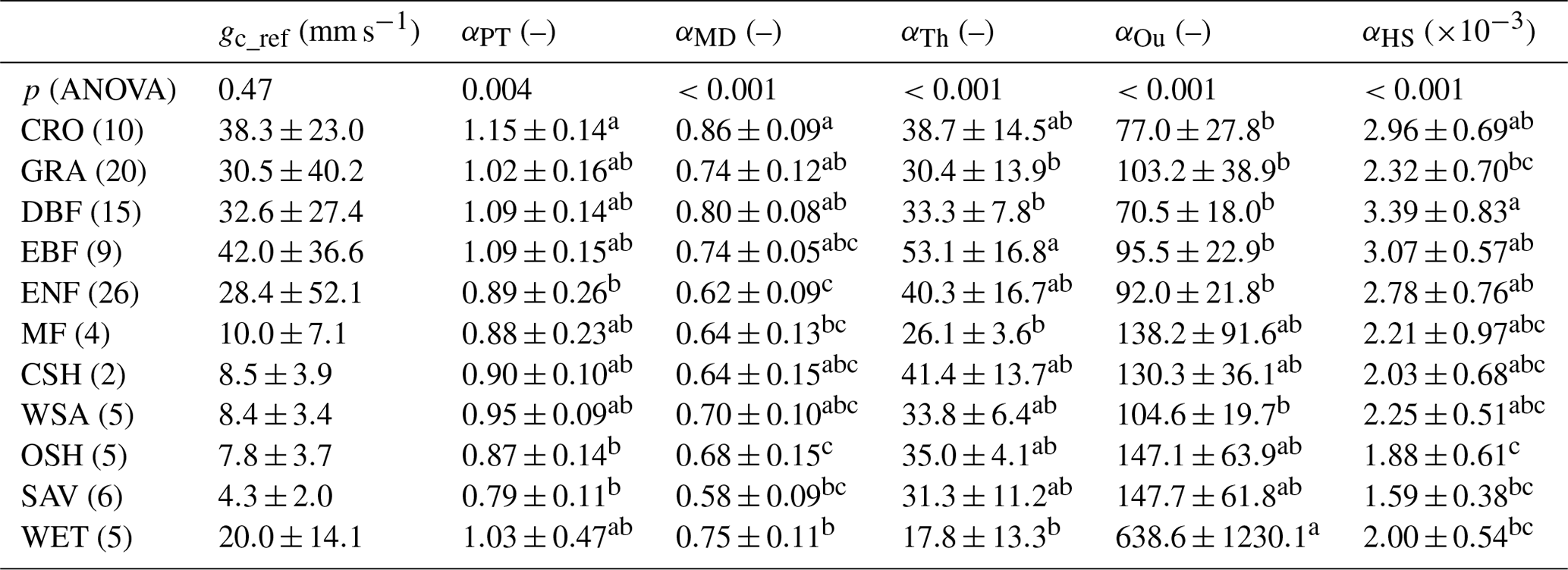
CRO: cropland; DBF: deciduous broadleaf forest; EBF: evergreen broadleaf forest; ENF: evergreen needleleaf forest; MF: mixed forest; CSH: closed shrubland; WSA: woody savannah; SAV: savannah; OSH: open shrubland; GRA: grasslands; WET: wetlands.

Table 3 Influence of atmospheric conditions on E_unstr and on selected key parameters (g_{c_ref}, α_PT, α_MD), based on unstressed days only defined using the energy balance criterion. Left: mean ±1 SD of the correlations of E_unstr, g_c, α_PT and α_MD against the atmospheric conditions. Right: number of sites (out of a total of 107) with significant negative/positive correlations between E_unstr, α_PT, g_{c_ref} and α_MD and the climate forcing variables.

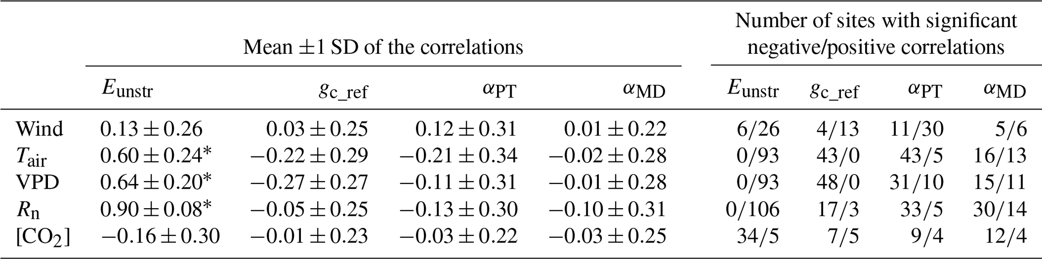
^* significantly different from 0.

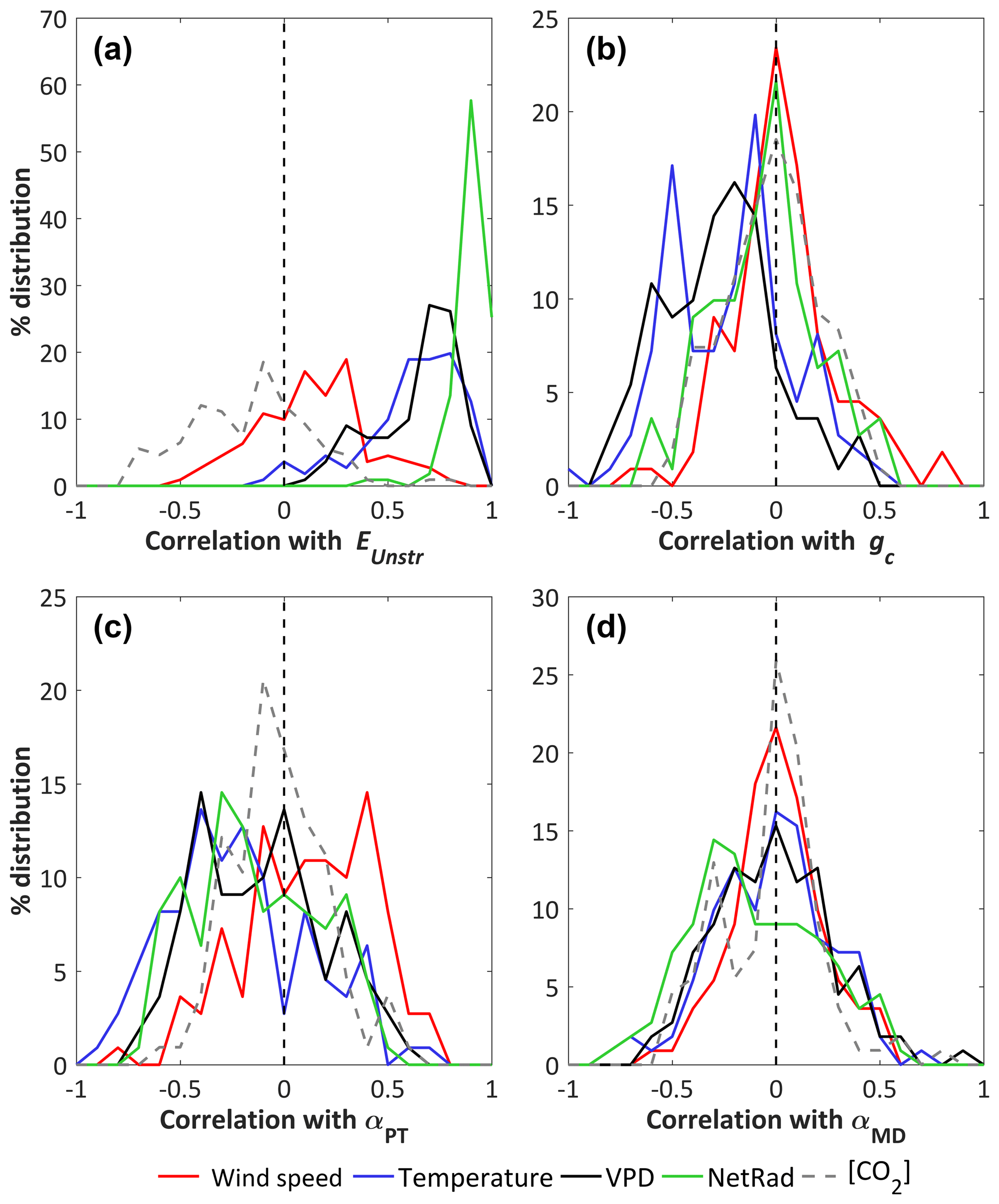
Figure 3 Histograms of correlations between the climate forcing variables and selected key parameters (a) E_unstr, (b) g_{c_ref}, (c) α_PT and (d) α_MD measured in all flux tower sites, based on unstressed days only defined using the energy balance criterion.

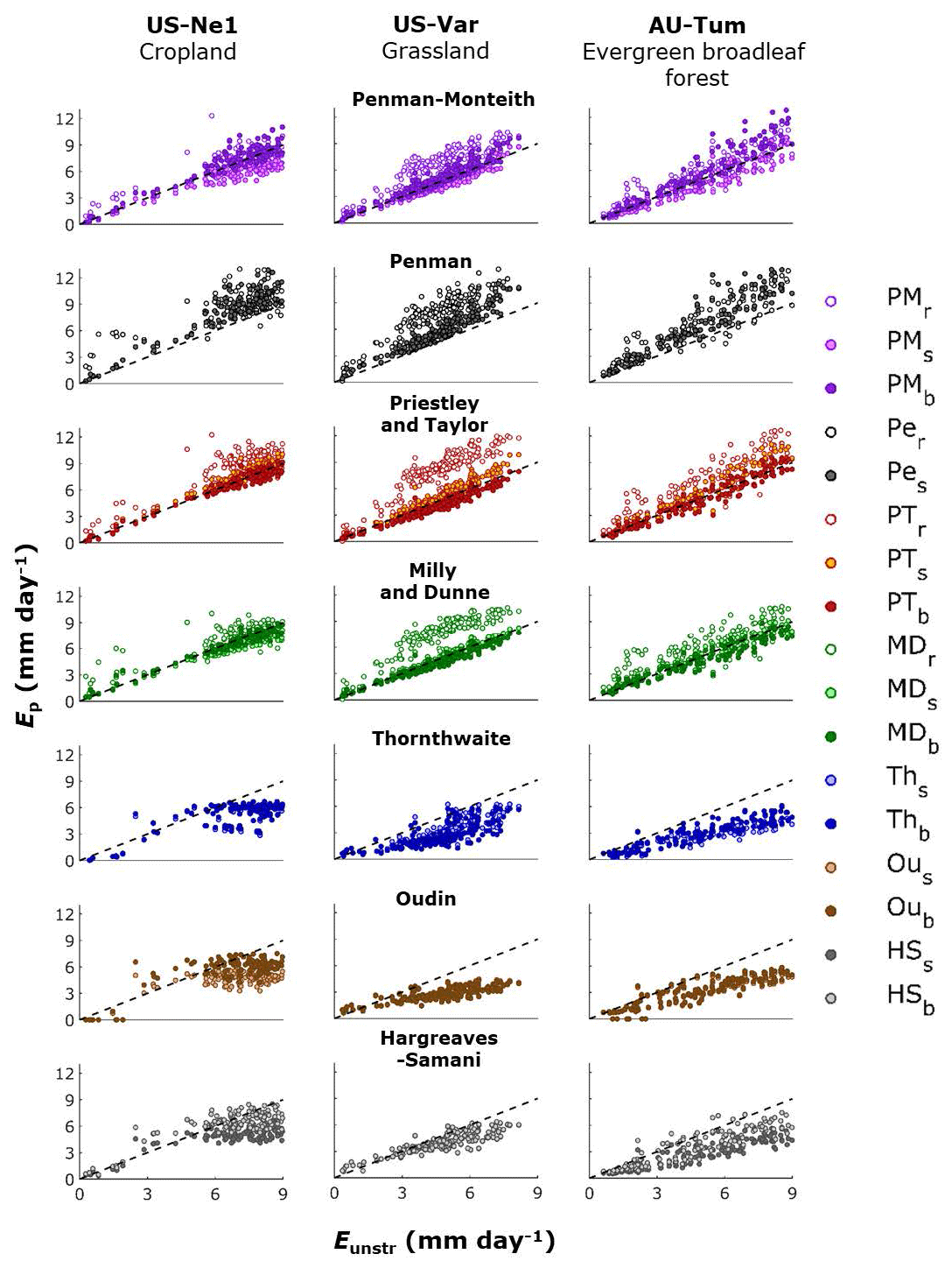
Figure 4 Scatterplot of the measured E_unstr versus E_p calculated with the different methods, based on unstressed days only, defined using the energy balance criterion. The discontinuous line is the 1:1 line.

Next, the effect of the atmospheric conditions on E_unstr and on the key parameters g_{c_ref}, α_PT and α_MD of the unstressed dataset is investigated. Figure 3 gives the distribution of the correlations between the climatic variables (R_n, T_a, VPD, u and [CO₂]) and E_unstr, g_{c_ref}, α_PT and α_MD of the unstressed records at each site. We did not include α_Th, α_HS or α_Ou because the temperature-based methods did not perform well (see Sect. 3.3). E_unstr was strongly positively correlated with R_n, T_a and VPD in most sites, but less with u (Fig. 3a, Table 3). Considering all sites, the correlation between g_{c_ref} and the climatic variables is not significantly different from zero for any climate variable, yet g_{c_ref} is significantly negatively correlated with T_air and with VPD in 40 % and 45 % of the flux tower sites, respectively (Table 3, Fig. 3b). The two other parameters, α_PT and α_MD, appear less correlated to any of the climatic variables across all sites (Table 3). In the case of α_MD, in particular, the distributions of the correlations against all climate forcing variables peak around zero (Fig. 3d): α_MD is hardly influenced by R_n and is overall not dependent on u, T_a, [CO₂] or VPD in most sites (Table 3).

3.3 Evaluation of different E_p methods

We first list the results of the analysis using the energy balance criterion for selecting the unstressed records (Sect. 2.4). The scatterplots of measured E_unstr versus estimated E_p based on the 17 different methods are shown in Fig. 4 for three sites belonging to different biomes. Despite the overall skill shown by the different E_p methods, considerable differences can be appreciated. In general, the methods designed for reference crops (PM_r, Pe_r, PT_r, MD_r) overestimate E_unstr and only two methods, MD_B and PT_B, match the measured E_unstr closely.

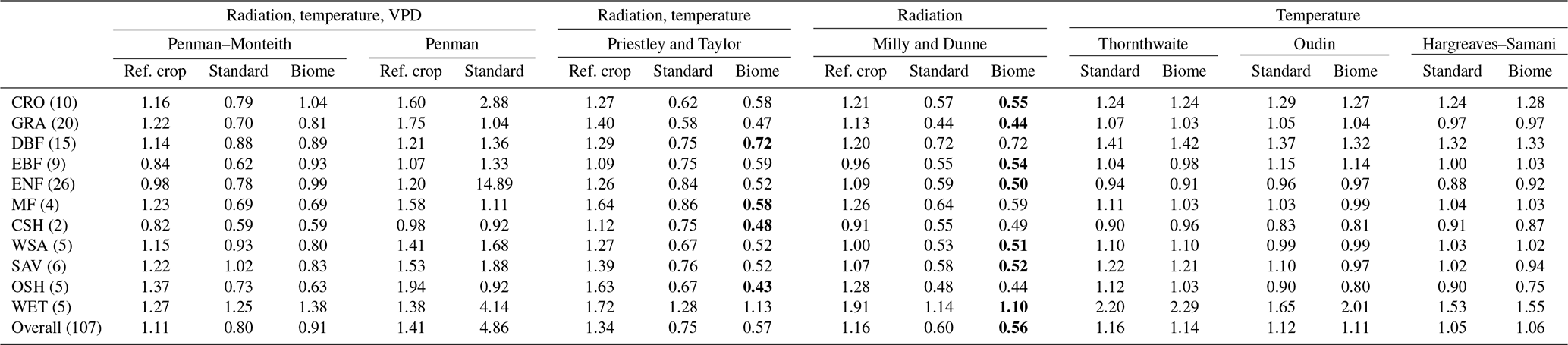
Table 4 Mean correlations per biome between the measured E_unstr and the different E_p methods, based on unstressed days only defined using the energy balance criterion. The methods with the highest correlation per biome are highlighted in bold. Different parts are used to group biomes into broader ecosystem types (in descending order: croplands, grasslands, forests, savannah ecosystems and wetlands).

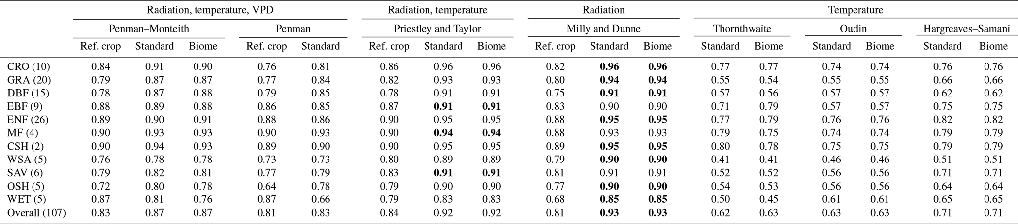
CRO: cropland; DBF: deciduous broadleaf forest; EBF: evergreen broadleaf forest; ENF: evergreen needleleaf forest; MF: mixed forest; CSH: closed shrubland; WSA: woody savannah; SAV: savannah; OSH: open shrubland; GRA: grasslands; WET: wetlands.

Table 4 gives the mean correlation per biome for each method. The results are very consistent and reveal that the highest correlations for nearly all biomes are obtained with the standard and biome-specific radiation-based method (MD_s and MD_b), closely followed by the standard and biome-dependent Priestley and Taylor method (PT_s and PT_b). Temperature-based methods have the lowest overall mean correlation as well as lower mean correlations per biome, with the Hargreaves–Samani method performing slightly better than the other two temperature-based methods. Note that the correlations are the same for the standard and biome-specific version in the case of the Priestley and Taylor (PT_s and PT_b), radiation-based (MD_s and MD_b), Oudin (Ou_s and Ou_b), and Hargreaves–Samani (HS_s and HS_b) methods (Table 4) – this is to be expected, as the only difference between the standard and biome-specific version of these methods is the value of their key parameters (α_PT, α_MD, α_Ou, α_HS), which are multiplicative (see Eqs. 3, 4, 6 and 7). Differences are however reflected in the unbiased root mean square error (unRMSE) and mean bias – see Tables 5 and 6. The biome-specific versions of the radiation-based method (MD_b) and of the Priestley and Taylor method (PT_b) consistently have the lowest unRMSE for all biomes. Though the difference between these two methods is small, MD_b performs slightly better. The standard Penman method (Pe_s) has the highest unRMSE. All reference crop methods (PM_r, Pe_r, PT_r, MD_r) have a mean unRMSE above 1 mm day⁻¹, and the temperature-based methods (Th_s, Ou_s, HS_s, Th_b, Ou_b and HS_b) also have a relatively high unRMSE. Finally, bias estimates are given in Table 6. Again, MD_b is overall the best-performing method (mean bias closest to 0 mm day⁻¹), closely followed by the PT_b method. Both methods consistently have the bias closest to zero among all biomes, except for wetlands. Most reference crop methods (PM_r, Pe_r, PT_r, MD_r), as well as Pe_s, overestimate E_p in all biomes.

Table 5 Unbiased root mean square error (unRMSE) (in mm day⁻¹) for the E_p methods per biome, based on unstressed days only defined using the energy balance criterion. The methods with the lowest unRMSE per biome are indicated in bold. Different parts are used to group biomes into broader ecosystem types (in descending order: croplands, grasslands, forests, savannah ecosystems and wetlands).

CRO: cropland; DBF: deciduous broadleaf forest; EBF: evergreen broadleaf forest; ENF: evergreen needleleaf forest; MF: mixed forest; CSH: closed shrubland; WSA: woody savannah; SAV: savannah; OSH: open shrubland; GRA: grasslands; WET: wetlands.

The use of soil water content as the criterion to select unstressed days (see Sect. 2.4) is explored. In total, 62 sites have soil water content data and meet the other selection criteria documented in Sect. 2.2. The results of this analysis are given in Tables S3–S5. To allow for a fair comparison, the same statistics have also been computed for just the same 62 tower sites with the energy balance criterion (Tables S6–S8). Using the soil moisture criterion, the correlations are overall lower and the results of the mean correlation, unRMSE and biases are less consistent. However, the overall performance ranking of the different models remains similar: PT_b is the best-performing method with overall the highest mean correlation (R=0.84) and the lowest unRMSE (0.78 mm day⁻¹) and a bias close to zero (−0.04), closely followed by the MD_b method, with R=0.81, unRMSE = 0.89 and a mean bias of −0.12. More complex Penman-based models, and especially the empirical temperature-based formulations, show again a lower performance.

So far, all flux sites were used to calibrate the key parameters (Table 2) and those same sites were also used for the evaluation of the different methods. This was done to maximise the sample size. However, to avoid possible overfitting, we also repeated the analysis after separating calibration and validation samples. For each biome, two-thirds of the sites were randomly selected as calibration sites and one-third as validation sites. The key parameters were then calculated from the calibration subset and applied to estimate E_p of the biome-specific methods of the validation subset. This procedure was repeated 100 times and the mean correlation, unbiased RMSE and bias per biome were calculated. Results show no substantial differences in overall correlation, unRMSE and bias of each method, which are provided in Tables S9–S11 for completeness.

Table 6 Mean bias (in mm day⁻¹) for the E_p methods per biome, based on unstressed days only defined using the energy balance criterion. The best-performing method per biome is indicated in bold. Different parts are used to group biomes into broader ecosystem types (in descending order: croplands, grasslands, forests, savannah ecosystems and wetlands).

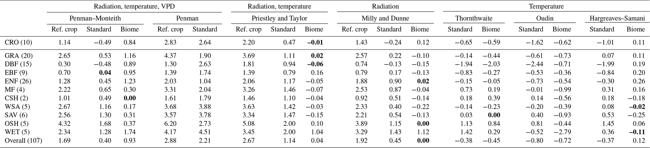
CRO: cropland; DBF: deciduous broadleaf forest; EBF: evergreen broadleaf forest; ENF: evergreen needleleaf forest; MF: mixed forest; CSH: closed shrubland; WSA: woody savannah; SAV: savannah; OSH: open shrubland; GRA: grasslands; WET: wetlands.

4 Discussion

4.1 Comparison of criteria to define unstressed days

We prioritised the energy balance over the soil moisture criterion to select unstressed days (see Sect. 2.4), because it can be applied to sites without soil moisture measurements and because it implicitly allows the exclusion of days in which the ecosystem is stressed for reasons other than soil moisture availability (e.g. insect plagues, phenological leaf-out, fires, heat and atmospheric dryness stress, nutrient limitations). In addition, soil moisture at specific depths can be a poor indicator of water stress, as rooting depth can vary and is not accurately measured (Powell et al., 2006; Douglas et al., 2009; Martínez-Vilalta et al., 2014). This is confirmed by our results: sampling unstressed days based on the energy-balance-based criterion resulted in higher correlations between E_p and E_unstr for all methods (Table S6 versus Table S3) and in lower unRMSE, with the exception of the temperature-based methods (Table S7 versus Table S4).

Nonetheless, it could be argued that, because the MD method assumes a constant evaporative fraction, the use of the evaporative fraction as a criterion for selecting unstressed days may favour the MD and even the closely related PT formulation. However, the soil moisture criterion adopted here provides an independent check of the results and confirms the robust and superior performance of the energy-driven PT_b and MD_b methods, independently of the framework chosen to select unstressed days. In the following discussion, the primary focus is on the results of selecting unstressed days based on the energy balance criterion.

4.2 Estimation of key ecosystem parameters

The resulting biome-specific values of the key parameters in Table 2 are within the range of values used in reference crop and standard applications of the models (Table 1), with the exception of α_PT, which is typically lower than the frequently adopted value of 1.26. Other studies also found α_PT values far below 1.26 but within the range of our study, mainly for forests (e.g. Shuttleworth and Calder, 1979; Viswanadham et al., 1991; Eaton et al., 2001; Komatsu, 2005) but also for tundra (Eaton et al., 2001) and grassland sites (Katerji and Rana, 2011) – see McMahon et al. (2013) for an overview. Our results and these studies demonstrate that the standard level of α_PT=1.26 is close to the upper bound and will lead to an overestimation of E_p at most flux sites (Table 5).

4.3 Lower performance of the Penman–Monteith method

The poor performance of the PM_r, PM_s and PM_b methods was relatively unexpected. Because the Penman–Monteith method incorporates the effects of T_a, VPD, R_n and u, it is often considered superior (e.g. Sheffield et al., 2012) and is even used as reference to evaluate other E_p formulations (e.g. Xu and Singh, 2002; Oudin et al., 2005b; Sentelhas et al., 2010). However, in studies dedicated to estimate E_a at eddy-covariance sites, in which g_c is adjusted so it reflects the actual stress conditions in the ecosystem, the Penman–Monteith method has already been shown to perform worse than other simpler methods, such as the Priestley and Taylor equation (e.g. Ershadi et al., 2014; Michel et al., 2016). It is well known that its performance depends on the reliability of a wide range of input data and on the methods used to derive r_aH and g_c (Singh and Xu, 1997; Dolman et al., 2014; Seiller and Anctil, 2016). In our case, the strict procedure followed to select the samples of 107 FLUXNET sites (see Sect. 2.2) ensured that all relevant variables were available, and the meteorological measurements were quality-checked. Hence, in our analysis, input quality is unlikely to be the cause of low performance.

We believe that the underlying assumption of a constant g_c, typically adopted by PM methods (PM_r, PM_s, PM_b) when estimating E_p, is a more likely explanation of the poor performance. PM was the only method in which the biome-specific calibration did not improve the performance. This is partially because of the large variation in g_{c_ref} among the different flux sites of the same biome type (Table 2). In addition, of all the key parameters, g_{c_ref} showed the largest mean relative standard deviation of the unstressed datasets of individual sites (results not shown). Surface conductance of the unstressed dataset was significantly negatively correlated with VPD in 45 % of the sites (Fig. 3b, Table 3). The relationship between g_c and VPD for two of these sites is illustrated in Fig. 5. It is clear that g_c of unstressed days (red dots) is always high for a given VPD, confirming the validity of the energy balance method. However, for these sites, it is also shown that g_c of the unstressed days becomes very high when VPD becomes very low. As a consequence, the mean value of g_c of the unstressed records, used to ultimately calculate g_{c_ref} per biome type, is highly influenced by local VPD and is not necessarily a representative ecosystem property.

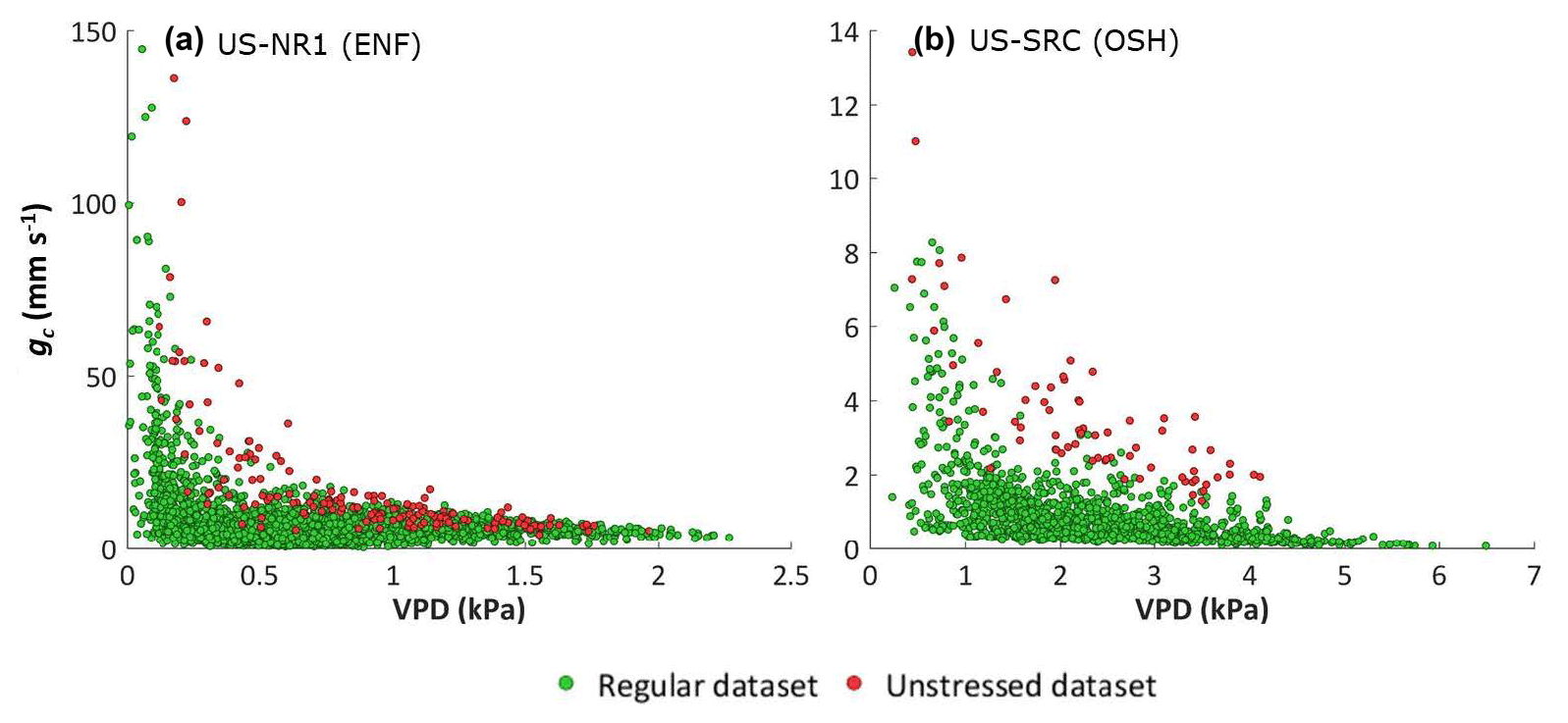
Figure 5 Surface conductance g_c as a function of vapour pressure deficit (VPD) of the regular and the unstressed datasets of two flux sites, (a) the evergreen needle forest Niwot Ridge Forest and (b) the open savannah woodland site Santa Rita Creosote.

The dependence of g_c on VPD, even when soil moisture is not limiting, has been well studied (e.g. Jones, 1992; Granier et al., 2000; Sumner and Jacobs, 2005; Novick et al., 2016) and incorporated in most conventional stomatal or surface conductance models (e.g. Jarvis, 1976; Ball et al., 1987; Leuning, 1995). Yet, out of practical reasons, g_{c_ref} is usually considered constant in E_p methods using the Penman–Monteith approach, with the PM_r as the best illustration. Our data confirm that in unstressed conditions stomata open maximally only when VPD is very low. As such, the VPD dependence of g_c smooths the impact of VPD in the Penman–Monteith equation – drops in VPD are compensated for by increases in g_c, and vice versa, lowering the impact of VPD on E_a (Eq. 1). As such, assuming a constant g_{c_ref} value overestimates the influence of VPD (and wind speed) on E_p.

Moreover, assuming a constant g_{c_ref} value in the Penman–Monteith method also ignores the influence of CO₂ levels on g_c. As a result, Milly and Dunne (2016) found that the Penman–Monteith methods with constant g_{c_ref} overpredicted E_p in models estimating future water use. Calibrating the sensitivity of g_{c_ref} to VPD and [CO₂] in the Penman–Monteith equation is outside the scope of this study, but could certainly improve E_p calculations – yet, it would further increase the complexity of the model. Finally, we note that the above discussion also applies to Penman's method: taking a wet canopy as reference in the Penman method (g_c=∞ or r_c=0) may not only overestimate E_p (Table 6) but also the influence of VPD and u on E_p.

4.4 Considerations regarding simple energy-based methods

The simpler Priestley and Taylor and radiation-based methods came forward as the best methods for assessing E_p with both criteria to define unstressed days. These observations are in agreement with studies highlighting radiation as the dominant driver of evaporation of saturated or unstressed ecosystems (e.g. Priestley and Taylor, 1972; Abtew, 1996; Wang et al., 2007; Song et al., 2017; Chan et al., 2018). They also agree with Douglas et al. (2009), who found that PT outperformed the PM method for estimating unstressed evaporation in 18 FLUXNET sites.

Both PT_b and MD_b are attractive from a modelling perspective, as they require minimum input data. However, this simplicity can also hold risks. The Priestley and Taylor method has been criticised for its implicit assumptions, which are also present in the MD_b method. For instance, by not incorporating wind speed explicitly, it is assumed that the effect of u on E_p is somehow embedded within α_PT (or α_MD). Yet, several studies indicate that wind speeds are decreasing (“stilling”) globally (McVicar et al., 2008, 2012; Vautard et al., 2010). McVicar et al. (2012) also reported an associated decreasing trend in observed pan evaporation worldwide as well as in E_p calculated with the PM_r method. With PT (or MD) methods, this trend cannot be captured. A similar criticism can be drawn with regards to the effect of [CO₂] on stomatal conductance, water use efficiency and thus potential evaporation (Field et al., 1995). A separate question is whether more complex E_p methods that incorporate the effects of u, [CO₂] or VPD explicitly do this correctly; the above-mentioned issues about the fixed parameterisation of the Penman–Monteith methods for estimating E_p indicate that this may typically not be the case.

Regarding the non-explicit consideration of u by simpler methods, our records show a limited effect of u on E_a and E_p, even when considering larger temporal scales. Of the 16 flux towers with at least 10 years of evaporation data, we calculated the yearly average E_a as well as the annual mean climatic forcing variables. Yearly averages were calculated from monthly averages, which in turn were calculated if at least three daytime measurements were available. Despite a relatively large mean standard deviation in yearly average u of 7.0 %, yearly average u was not significantly correlated with E_a in any of these sites. In contrast, yearly average R_n was positively correlated with yearly average E_a in 7 of the 16 sites, with comparable mean standard deviation in annual R_n (8.5 %). Moreover, looking at all individual towers and using the daily estimates, neither α_MD nor α_PT were correlated with u (Fig. 3c and d, Table 3). In fact, since α_MD appears hardly affected by any climatic variable, and given the relatively small range in α_MD values within each biome (Table 2), it appears that α_MD is a robust biome property that can be used in the seamless application of these methods at a global scale. The robustness of α_MD as a biome property is furthermore confirmed by the analysis with independent calibration and validation sites, which hardly affected the unRMSE and bias (Tables S10 and S11).

4.5 Use of available energy under stress conditions

The best-performing methods rely heavily on measurements of available energy (R_n−G) (Eqs. 2 and 3). In Sect. 3.2, all E_p calculations used available energy obtained during unstressed conditions. The question is whether E_p can also be calculated correctly using the actual R_n and G when the ecosystems are not unstressed. As mentioned in Sect. 1, there is discussion on whether SW_out and LW_out should be considered forcing variables or ecosystem responses (e.g. Lhomme, 1997; Lhomme and Guilioni, 2006; Shuttleworth, 1993). Among other considerations, it is clear that T_s will be lower if vegetation is healthy and soils are well-watered (Maes and Steppe, 2012), which results in lower LW_out and higher R_n. Therefore, while using the observations of SW_in and LW_in as forcing variables in the computation of E_p is defendable (despite the potential atmospheric feedbacks that may derive from the consideration of unstressed conditions), we agree that SW_out, LW_out and G should ideally reflect unstressed rather than actual conditions to estimate E_p. Note that, in that case, E_p deviates from $E_{{\mathrm{p}}_{\mathrm{0}}}$ in the complementarity relationship, in which atmospheric feedbacks affecting incoming radiation or VPD are implicitly considered (Kahler and Brutsaert, 2006).

A method to derive the unstressed estimates of SW_in (through the albedo, α), LW_in (through T_s) and G under stressed conditions is presented in the Sect. S2 and is based on the MD_b method and on flux data of the unstressed datasets. We further refer to this method as the “unstressed” E_p. It requires a large amount of input data and is not practically applicable at a global scale. Comparing the mean unstressed E_p with the “actual” E_p (i.e. E_p calculated from the actual R_n and G) for all sites reveals that the actual E_p is 8.2±10.1 % lower than the unstressed E_p. There are no significant differences between biomes, but the distribution of the underestimation is left-skewed and the actual E_p is more than 10 % lower than the unstressed E_p in 22 % of the sites (Fig. 6). The main reason explaining about 65 % of the difference between the actual and the unstressed E_p is the difference in T_s. Assuming that the unstressed T_s can be estimated as the mean of T_a and the actual T_s results in a straightforward alternative to approximate the unstressed E_p with only data of T_a and radiation:

$$\begin{array}{ll}{\displaystyle }{E}_{\mathrm{p}}& {\displaystyle }={\mathit{\alpha }}_{\mathrm{MD}}\left((\mathrm{1}-\mathit{\alpha }){\mathrm{SW}}_{\mathrm{in}}+\mathit{\epsilon }{\mathrm{LW}}_{\mathrm{in}}-\mathrm{0.5}\mathit{\epsilon }{\mathrm{LW}}_{\mathrm{out}}\right.\\ \text{(17)}& {\displaystyle }& {\displaystyle }\left.-\mathrm{0.5}\mathit{\epsilon }\mathit{\sigma }{T}_{\mathrm{a}}^{\mathrm{4}}-G\right).\end{array}$$

This approach was also tested and resulted in a mean underestimation of E_p of 2.6±5.8 % compared to the unstressed E_p, with a mean median value at −0.1 % (Fig. 6). Given the low error and the straightforward calculation, we recommend this method to calculate E_p at global scales.

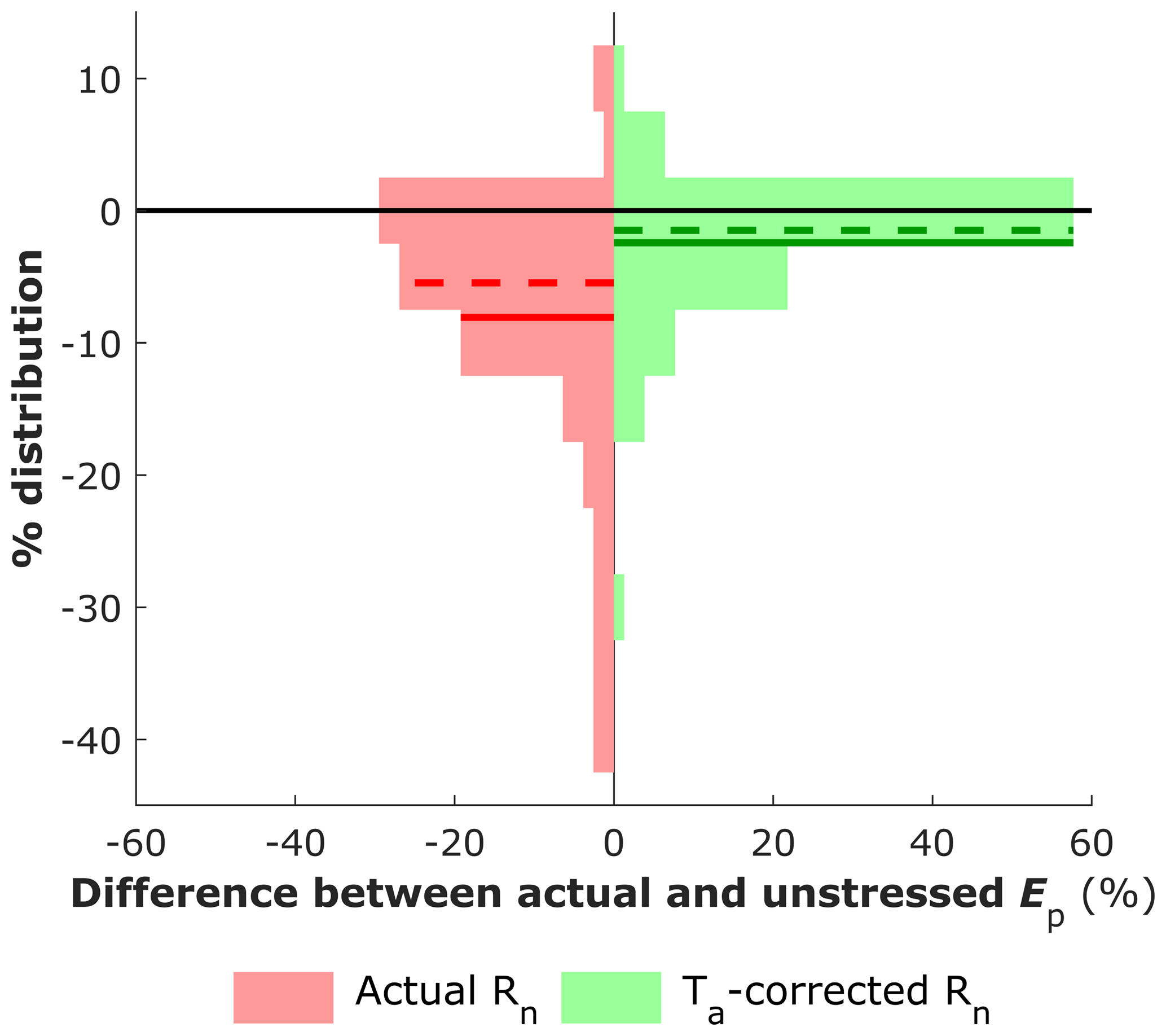
Figure 6 Comparison of the E_p calculated with a modelled method calculating (R_n−G) for unstressed conditions (Sect. S2) using flux tower data, and the actually observed (R_n−G) (red) or a simplified correction of (R_n−G) using T_a (Eq. 17) (green). Negative y values indicate a lower estimation of E_p compared to the modelled method. For each distribution, the mean and median are indicated with a full and dashed line, respectively.

Figure 7 Seasonal evolution of E_a (top, green), E_p (top, red) and the S factor ($S=E_{\mathrm{a}}{E}_{\mathrm{p}}^{-\mathrm{1}}$, confined between 0 and 1) for two ecosystems: (a) a grassland crop, Sturt Plains in Australia; and (b) a deciduous broadleaf forest, Ohio Oak forest in the USA. E_p was calculated with the MD_b method and using the tower-based correction of (R_n−G) as presented in S2 of the Supplement.

Figure 7 gives an example of the seasonal evolution of E_a and E_p and the S factor ($S=E_{\mathrm{a}}{E}_{\mathrm{p}}^{-\mathrm{1}}$) in a grassland (Fig. 7a) and a deciduous forest site (Fig. 7b). The short growing season in the grassland site, when E_a is close to E_p and values of S are close to 1, stands in clear contrast with the winter period, when grasses have died off and E_a and consequently also S are very low. In the relatively wet broadleaf forest, E_a and E_p follow a similar seasonal cycle. In winter, when total evaporation is limited to soil evaporation, S is very low; in spring, when leaves are still developing, E_a lags E_p. In summer, S remains high and close to one.

5 Conclusion

Based on a large sample of eddy-covariance sites from the FLUXNET2015 database, we demonstrated a higher potential of radiation-driven methods calibrated by biome type to estimate E_p than of more complex Penman–Monteith approaches or empirical temperature-based formulations. This was consistent across all 11 biomes represented in the database and for two different criteria to identify unstressed days, one based on soil moisture and the other on evaporative fractions. Our analyses also showed that the key parameters required to apply the higher-performance radiation-driven methods are relatively insensitive to climate forcing. This makes these methods robust for incorporation into global offline models, e.g. for hydrological applications. Finally, we conclude that, at the ecosystem scale, Penman–Monteith methods for estimating E_p should only be prioritised if the unstressed stomatal conductance is calculated dynamically and high accuracy observations from the wide palate of required forcing variables are available.

Appendix A

Table A1 Abbreviation list.