Estimating irrigation water use over the contiguous United States by combining satellite and reanalysis soil moisture data

Effective agricultural water management requires accurate and timely information on the availability and use of irrigation water. However, most existing information on irrigation water use (IWU) lacks the objectivity and spatiotemporal representativeness needed for operational water management and meaningful characterization of land–climate interactions. Although optical remote sensing has been used to map the area affected by irrigation, it does not physically allow for the estimation of the actual amount of irrigation water applied. On the other hand, microwave observations of the moisture content in the top soil layer are directly influenced by agricultural irrigation practices and thus potentially allow for the quantitative estimation of IWU. In this study, we combine surface soil moisture (SM) retrievals from the spaceborne SMAP, AMSR2 and ASCAT microwave sensors with modeled soil moisture from MERRA-2 reanalysis to derive monthly IWU dynamics over the contiguous United States (CONUS) for the period 2013–2016. The methodology is driven by the assumption that the hydrology formulation of the MERRA-2 model does not account for irrigation, while the remotely sensed soil moisture retrievals do contain an irrigation signal. For many CONUS irrigation hot spots, the estimated spatial irrigation patterns show good agreement with a reference data set on irrigated areas. Moreover, in intensively irrigated areas, the temporal dynamics of observed IWU is meaningful with respect to ancillary data on local irrigation practices. State-aggregated mean IWU volumes derived from the combination of SMAP and MERRA-2 soil moisture show a good correlation with statistically reported state-level irrigation water withdrawals (IWW) but systematically underestimate them. We argue that this discrepancy can be mainly attributed to the coarse spatial resolution of the employed satellite soil moisture retrievals, which fails to resolve local irrigation practices. Consequently, higher-resolution soil moisture data are needed to further enhance the accuracy of IWU mapping.

1 Introduction

The agricultural sector uses over 70 % of global freshwater withdrawals for irrigation (Shiklomanov, 2000; Foley et al., 2011). As a result of world population increase and rising living standards, water will be a major constraint for agriculture in the coming decades. In addition, climate change will likely have a profound impact on irrigation demand throughout the world. The projected increase in global mean temperature and changing precipitation patterns are expected to decrease natural water availability in already-water-scarce regions of the world (Vörösmarty et al., 2000; Rockström et al., 2012; Kummu et al., 2016). For instance, Döll (2002) showed that around two-thirds of the areas that were irrigated in 1995 will require more irrigation water by 2070. Moreover, predictions show that the hydrological cycle will intensify. Hence, drought and flood events are expected to occur both more frequently and severely, which further impairs water availability for agriculture (Allan and Soden, 2008).

On the other hand, irrigation itself is an important anthropogenic climate forcing (Sacks et al., 2009). It influences the surface water and energy balance through directly increasing soil moisture (SM). In turn, soil moisture is widely known to modulate the partitioning of energy between sensible and latent heat (Seneviratne et al., 2010). Subsequently, irrigation cools the land surface on local to regional scales through increasing evapotranspiration (ET), whereas the increased availability of atmospheric water vapor can enhance cloud cover and precipitation (Boucher et al., 2004; Lobell et al., 2006; Sacks et al., 2009). Researchers agree that irrigation may have masked the full warming signal caused by greenhouse gas emissions (Bonfils and Lobell, 2007; Kueppers et al., 2007). As a past expansion of irrigated area and an overall increase in irrigation intensity may have significantly affected surface temperature observations, it is crucial to include irrigation impacts both in understanding historical climate and modeling future climate trends (Lobell et al., 2006). Assuming a similar expansion of irrigation as in recent decades, some regions may actually benefit from this irrigation cooling effect. As outlined in Ozdogan et al. (2006), ET and in turn irrigation water requirements can decrease within agricultural microclimates. However, nonlinear repercussions on temperature extremes can be expected when the required water supply cannot be met (Thiery et al., 2017) and (semi-)arid regions are generally expected to be adversely affected by water scarcity (Kueppers et al., 2007). As a consequence, especially in water-scarce regions, government agencies and water managers are challenged to increase water use efficiency, optimize the distribution of water among farms and detect illegal groundwater pumping activities (Siebert et al., 2010; Taylor et al., 2012). For example, as a consequence of prolonged winter precipitation deficits and positive temperature anomalies from 2012 to 2017, a record-breaking drought peaking in 2015 affected the California Central Valley. While farmers tried to compensate for the 2015 surface water shortage by pumping more groundwater, a net water shortage of over 3 km³ resulted in the fallowing of approximately 230 000 ha of land (Howitt, 2015).

To date, irrigation practices are typically not explicitly included in land surface, climate or weather models. On the other hand, irrigation directly impacts land surface temperature, humidity and soil moisture observations, and through them irrigation indirectly impacts model simulations when they are being assimilated (Tuinenburg and Vries, 2017). A range of climate modeling studies employed irrigation modules on a global scale. Mainly based on a combination of static spatial maps of irrigated area and soil moisture and/or vegetation data, they tried to approximate seasonal IWU (Lobell et al., 2006; Bonfils and Lobell, 2007; Kueppers et al., 2007). However, the simulated impact of irrigation on both global and regional climate showed considerable variation across studies. With respect to a contiguous US (CONUS) domain, Lawston et al. (2015) assessed the effects of drip, flood and sprinkler irrigation methods during a climatically dry and wet year on land–atmosphere interactions. They used the National Aeronautics and Space Administration's (NASA) high-resolution Land Information System (LIS) and the NASA Unified Weather Research and Forecasting Model framework both in offline and coupled simulations. In accordance with previous studies, they found that irrigation indeed cools and moistens the surface over and downwind of irrigated areas. Moreover, they found that the magnitude of this irrigation cooling effect strongly depends on the parametrization of the respective irrigation methods. In a very recent study, Kumar et al. (2018) conducted a multi-sensor, multivariate land data assimilation experiment over the CONUS by using the NASA LIS to enable the National Climate Assessment Land Data Assimilation System. Particularly, the use of a larger-than-normal range of soil moisture data records and snow depth data from microwave remote sensing combined with an irrigation intensity map systematically improved soil moisture and snow depth simulations.

With respect to the discrepancies in the global modeling studies, Sacks et al. (2009) argued that they can be primarily explained by systematic differences in the control of irrigation water application within the respective modules, e.g., by climate, food demand and economical conditions. Logically, this arguments also holds true for the modeling study by Lawston et al. (2015). Regarding the irrigation forcing used in Kumar et al. (2018), we argue that the term “irrigation intensity” gives a false impression. Irrigation intensity in a physical sense should not be attributed to fractional irrigated area but must rather be connected to the actual irrigation water use (IWU) per unit area. In addition, fields may be either over- or under-irrigated with respect to the physically “ideal” amount. Hence, current irrigation modules are unable to consistently reflect real-world conditions and thus introduce uncertainties in modeling and data assimilation. Consequently, information on the spatiotemporal distribution and development of actual IWU is needed to improve the representation of land–atmosphere feedbacks in model simulations (Ozdogan et al., 2010a).

1.1 Statistics on irrigated areas and water withdrawals

Available information on irrigated areas, and particularly irrigation water use, lacks objectivity, spatial consistency and temporal resolution needed for large-scale hydrological assessments and modeling (Deines et al., 2017). On local to regional scales, some irrigation districts conduct regular surveys, but often the data are not publicly available, lack geo-referencing and are difficult to compare between regions due to different sampling techniques. The elementary sources of large-scale irrigation data are national and subnational statistical units, which in most countries routinely collect information on irrigated area and/or irrigation water withdrawals (IWW). Data are usually represented as area equipped for irrigation (AEI) and in some cases also reflect the area actually irrigated (AAI) in the respective year of the census (Siebert et al., 2005). The Global Map of Irrigation Areas (GMIA) was the first global-scale geospatial irrigated area data set (Döll, 2002; Döll and Siebert, 2002) based on such statistics. GMIA combines subnational irrigation data from various sources (FAO, UN, World Bank, agriculture departments) and geospatial information on the location and extent of irrigation schemes (point, polygon and raster data, land cover maps and satellite imagery) to map AEIs and AAIs at 0.5^∘ resolution around the year 2000. In subsequent versions the resolution was improved to 5 armin ×5 arcmin (Siebert et al., 2005, 2007) and a new global historical irrigation data set providing time series of AEI between 1900 and 2005 was developed (Siebert et al., 2015). However, the large variability in the quality of the underlying statistical inventory data is propagated into the uncertainty of the final spatial map (Siebert et al., 2005).

In summary, the main limitations of statistical inventories and derived products are the following.

1. The quality of the data varies significantly among countries (Siebert et al., 2010). While for instance the United States agricultural census is considered to have high quality, many developing countries lack the resources for comprehensive reporting.

2. National statistics are usually only valid for single years and depend on the individual compilation cycle of each country (e.g., every 5 years in the case of the US).

3. Irrigated area estimates usually reflect areas equipped for irrigation, rather than areas actually irrigated. Depending on climatic and market conditions, farmers may decide to only cultivate and irrigate a portion of their fields.

4. Irrigation volume estimates reflect irrigation water withdrawals rather than actual irrigation water use (e.g., if rainfall is sufficient, already withdrawn spare water is stored in reservoirs instead of being irrigated).

5. Naturally, survey-based statistics are only based on a sample of farms, which may not be representative.

6. Conventional methods are unable to reflect illegally withdrawn water used for irrigation (Roseta-Palma et al., 2014; Saffi and Cheddadi, 2010).

On the basis of these drawbacks, remote sensing evolved as an effective tool to potentially overcome these limitations since it provides synoptic, independent and timely information of biogeophysical variables that are either directly or indirectly related to irrigation.

1.2 Remote sensing for irrigation mapping

1.2.1 Optical and thermal remote sensing

Data acquired by optical sensors (AVHRR, MODIS, Landsat) have been extensively used to identify irrigated areas on local, regional and global scales. Vegetation indices have been identified as effective proxies for irrigation practices, because irrigated and non-irrigated croplands show different spectral responses during the peak growing season (Ozdogan et al., 2010b). A wide range of studies used vegetation indices to map annual irrigated areas and their changes through time, sometimes in combination with statistical inventory data.

Only few global land-use–land-cover (LULC) maps based on optical remote sensing separate irrigated from rain-fed croplands. For example, the United States Geological Survey (USGS) Global Land Cover Characteristics (GLCC) data set was derived from 1 km Advanced Very High Resolution Radiometer (AVHRR) sensor data and identified four types of irrigated croplands in the year 1992 (Loveland et al., 2000). However, the classification algorithms used were not tailored to irrigated area mapping, thus resulting in low classification accuracies. Large discrepancies were found between USGS GLCC and country-level reports of irrigated area, originating from both the uncertainties of the inventory data and technical limitations of the remote sensing data sets (Vörösmarty et al., 2000). Through a combination of unsupervised clustering and expert knowledge, the European Space Agency (ESA) Climate Change Initiative (CCI) has produced a global land cover product at 300 m resolution using Medium Resolution Imaging Spectrometer (MERIS) data (Bontemps et al., 2013). It distinguishes between irrigated and non-irrigated croplands for 2000, 2005 and 2010. However, we argue that over the CONUS the irrigated class is likely to be considered unreliable, as apparently all irrigated lands are wrongly attributed to the non-irrigated agriculture class.

Other studies used approaches specifically tailored to irrigated area mapping. For instance, the global data set of monthly irrigated and rain-fed crop areas around the year 2000 (MIRCA2000) provides irrigated and rain-fed areas for 26 crop classes for each month of the year at 5 arcmin resolution (Portmann et al., 2010). For this purpose, agricultural census statistics, national reports, databases, a map of crop-specific annual harvested area, a cropland extent map, the GMIA, crop calendars, and ancillary information on climate and topography were combined. Using quantitative spectral matching techniques on normalized difference vegetation index (NDVI) time series from multiple sensors (AVHRR, SPOT-1, MODIS, Landsat 7 and JERS-1 SAR) in combination with climate (monthly precipitation and temperature data from the Climate Research Unit) and ancillary data (GTOPO30 1 km digital elevation model, global tree cover), the International Water Management Institute (IMWI) produced a Global Irrigated Area Map (GIAM) at 1 km resolution around the year 2000 (Thenkabail et al., 2009). More recently, Salmon et al. (2015) created a global map of rain-fed, irrigated and paddy croplands (GRIPC) around the year 2005 at 500 m spatial resolution using supervised classification of remote sensing, climate and agricultural inventory data. However, there are large discrepancies between the different global data sets mainly stemming from varying definitions of irrigated areas among the data sets (i.e., area equipped for irrigation, irrigated area and cropped area) and differing reference years (i.e., the years 2000 and 2005) (Salmon et al., 2015; Meier et al., 2018). Moreover, three of the four existing global maps (GMIA, MIRCA2000 and GRIPC) rely on agricultural inventory data for the classification of irrigated areas, which is subject to major limitations concerning quality and accuracy. In addition, the maps are limited to single years (GMIA, GIAM, GRIPC) or single months within a single year (MIRCA2000), thus not being able to address the high inter-annual variability of irrigated areas, which is mainly governed by climate and market conditions (Deines et al., 2017).

On a continental scale, the MODIS Irrigated Agriculture Dataset for the conterminous United States (MIrAD-US) was created by assimilating county-level irrigation statistics with MODIS-derived seasonal peak NDVI to spatially identify irrigated and non-irrigated lands at 250 m resolution (Ozdogan and Gutman, 2008; Pervez et al., 2008; Pervez and Brown, 2010). A significant drawback is that the map compilation is tied to the same 5-year cycle of the United States Department of Agriculture (USDA) Census of Agriculture. Ambika et al. (2016) mapped irrigated areas from 2000 to 2015 at 250 m resolution over India by using 250 m MODIS seasonal peak NDVI data and 56 m LULC data. Teluguntla et al. (2017) used spectral matching techniques and automated cropland classification algorithms to infer cropland extent, irrigated versus rain-fed croplands, and cropping intensities over Australia. The latter two products allow for the study of inter-annual variability of irrigated areas (Ambika et al., 2016).

On a regional scale, higher-resolution Landsat imagery was adopted by a range of studies. Ozdogan et al. (2006) used 30 m Landsat imagery to map changes in annual irrigated area from 1993 to 2002 in southeastern Turkey based on NDVI thresholding approaches and compared them with estimates of irrigation water requirements inferred from potential evapotranspiration. In a recent study, Deines et al. (2017) produced annual irrigation maps for 1999–2016 for a region in the High Plains aquifer (United States) at 30 m resolution. Pun et al. (2017) used a combination of surface energy balance partitioning and vegetation indices to classify irrigated and non-irrigated croplands at 30 m resolution in Nebraska.

Thermal remote sensing has been widely used to map irrigation water based on estimating potential evaporation from surface energy heat fluxes and the application of specific crop factors (Rosas et al., 2017). A well-known technique is the Surface Energy Balance Algorithm for Land, which estimates variables of the hydrological cycle based on remotely sensed surface energy balance components (Bastiaanssen et al., 1998). In contrast, Hain et al. (2015) developed a novel method for inferring regions where non-precipitation inputs (e.g., irrigation) significantly impact terrestrial latent heat flux (LE). They compared modeled bottom-up LE (i.e., without irrigation) and top-down LE drawn from observations of diurnal land surface temperature changes which are connected to changes in the land surface moisture status and therefore irrigation. However, these methods are only able to provide estimates on irrigation water requirements (i.e., what amount of water a plant would ideally need), as opposed to actually irrigated water, as in practice fields are often under-irrigated.

1.2.2 Microwave remote sensing

Microwave observations are widely used to estimate soil moisture (Entekhabi et al., 2010; Wagner et al., 2013; Dorigo et al., 2017). The major advantages of microwave observations are their all-weather capability and the intrinsic capacity to sense a geophysical variable which is directly and physically linked to irrigation.

The first study to investigate the utility of satellite soil moisture retrievals for irrigation mapping was carried out by Kumar et al. (2015). They used soil moisture retrievals from ASCAT, AMSR-E, SMOS and WindSat, and the ESA CCI multi-satellite surface soil moisture product in combination with soil moisture estimates from the Noah LSM (land surface model) to map irrigated areas in the CONUS. Their key assumption was that irrigation is not included in the formulation of LSM, whereas satellite-derived soil moisture is expected to reflect the changes in soil moisture induced by irrigation. Based on synthetic data, they were able to detect differences between the probability density functions of satellite and modeled soil moisture. However, the satellite data showed only few systematic differences that could be reliably related to irrigation practices.

Qiu et al. (2016) compared trends from 1996 to 2010 in China of ESA CCI, ERA-Interim/Land reanalysis and in situ soil moisture, as well as precipitation. They observed significant discrepancies between precipitation and satellite soil moisture trends over irrigated areas, which they ascribed to irrigation. Escorihuela and Quintana-Seguí (2016) compared three global satellite soil moisture products (ASCAT, AMSR2 and SMOS) with model soil moisture estimates from the Surface Externalisée (SURFEX) model (Masson et al., 2013) (forced with meteorological data) in the Mediterranean. Only a downscaled version of SMOS (SMOScat) showed significantly lower correlations over irrigated areas. The authors argued that primarily due to the coarse spatial resolution of the native soil moisture retrievals the other products were not able to resolve the irrigation signal from the soil moisture signal from the surrounding dry-land area. Very recently Lawston et al. (2017) investigated the potential of the new SMAP (Soil Moisture Active Passive mission) enhanced 9 km SM product to identify irrigation signals in three semi-arid regions in the western United States. Results showed that SMAP soil moisture carries a clear irrigation signal from rice irrigation in the Sacramento Valley (California), while the signals were less obvious in the other two regions (Columbia River basin, Washington and Colorado).

1.3 Objective of this study

Despite the large number of studies using remote sensing approaches to map irrigated area and irrigation water requirements at various spatial and temporal scales, none of these approaches has attempted to derive actual irrigation water use. To bridge this gap, we propose a new method for estimating IWU from a combination of remotely sensed and modeled reanalysis soil moisture data. The approach is based on the hypothesis that neither the structure nor the forcing of the model data accounts for artificial water supply, while the microwave soil moisture retrievals do (Kumar et al., 2015; Escorihuela and Quintana-Seguí, 2016). The method is implemented over the CONUS by using three state-of-the-art microwave soil moisture products (i.e., based on SMAP, AMSR2 and ASCAT) in combination with MERRA-2 reanalysis soil moisture. By using passive L-band and both active and passive C-band soil moisture data, we aim to assess the impact of the microwave observation frequency and the sensing technique with respect to irrigation quantification. For this reason we only used one data set per category.

The paper is organized as follows: Sect. 2 provides a general overview of the irrigation landscape in the CONUS. Section 3 covers the utilized satellite, model and ancillary data sets and the preprocessing involved. The theoretical and practical aspects of the new methodology to estimate IWU are discussed in Sect. 4. Results are shown and discussed with respect to official reference irrigation data in Sect. 5. Section 6 concludes the study and gives an outlook on follow-on research.

2 Study area

2.1 Irrigation practices in the contiguous United States

The amount of water needed by a certain crop for optimal growth mainly depends on three factors: crop type, soil and climate. Irrigation water need is given by the difference between these requirements for optimal crop growth and effective rainfall. In the largely semi-humid climate of the eastern United States, irrigation is supplemental, which means that irrigation is applied to mostly rain-fed crops during times of insufficient rainfall to achieve higher yields than under rain-fed conditions alone. In contrast, the predominantly semi-arid climate of the western US makes artificial water supply a necessity, thus requiring full irrigation.

The 2013 Farm and Ranch Irrigation Survey (FRIS) of the National Agricultural Statistics Service (NASS) of the USDA provides selected irrigation data from surveys conducted at approximately 35 000 farms using irrigation across the US (USDA, 2013). It reports state-level data of both irrigated area and irrigation water withdrawals subdivided by specific crop type, water source and irrigation technique. In addition, these estimates are given for crops cultivated outdoors (“in the open”) and indoors (“under protection”, e.g., horticultural crops grown in greenhouses). Figure 1 shows the per-state irrigated area and irrigation water withdrawals limited to crops grown outdoors, as well as irrigation application rates during the 2013 growing season provided by FRIS.

Figure 1 Per-state irrigated area, irrigation water withdrawals and irrigation water application rates for 2013. The data were drawn from the latest Farm and Ranch Irrigation Survey (FRIS) and only reflect irrigation operations in open fields (e.g., excluding crops grown and irrigated in greenhouses).

It is likely that the sensitivity of satellite soil moisture retrievals to irrigation increases when the irrigation application efficiency of a particular irrigation system or technique deteriorates. Therefore, we expect higher sensitivity towards gravity irrigation systems (e.g., flood and furrow irrigation) and lower sensitivities towards sprinkler and micro-irrigation systems. Figure A1 shows a distinct decline in irrigation rates per area from the semi-arid west to the more humid east. The state of Arizona has the highest irrigation rate per area, followed by California and Nevada. Gravity flow systems show the highest rates in California and Arizona but also depict large values along the Mississippi Delta. This can mainly be attributed to the cultivation of rice, which is primarily grown in these regions and is either flood or furrow irrigated. Finally, micro-irrigation systems are largely limited to the western half of the US.

2.2 Focus areas

In addition to the continental-scale analysis, we chose four irrigation hot spots characterized by different climates and irrigation practices within the CONUS (Fig. 2) to comprehensively assess the spatiotemporal dynamics of irrigation. These regions are the Sacramento Valley and San Joaquin Valley in the California Central Valley; the Snake River Plain, Idaho; the High Plains, Nebraska; and part of the Mississippi Floodplain located within the state of Mississippi. For each focus area, we conducted a time series analysis at a local scale (Sect. 5.3), as well as a cross comparison with reference data on irrigated area (Sect. 5.5) and irrigation water withdrawals (Sect. 5.4).

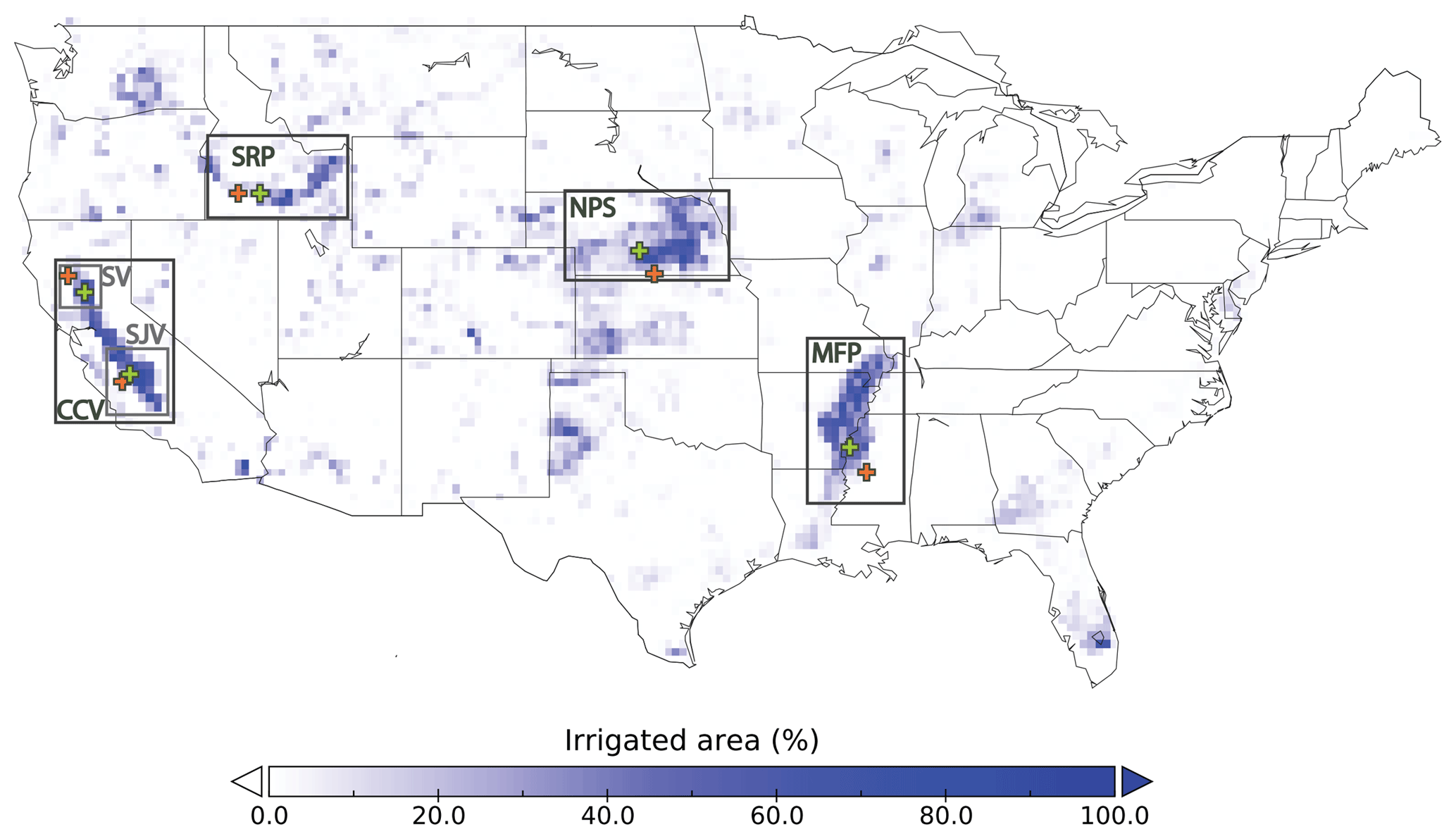
Figure 2 Study regions and locations of the pixels selected for a local time series analysis over the fractional irrigated area map derived from the spatially aggregated MIrAD-US data set (Pervez and Brown, 2010). The focus regions are included in black squares and include the Sacramento Valley (SV) and San Joaquin Valley (SJV) in the California Central Valley (CCV), Snake River Plain (SRP), Nebraska Plains (NPS) and the Mississippi Floodplain (MFP). Green and orange crosses indicate the locations of the irrigated (PI) and non-irrigated (PNI) pixels, respectively, at which we further analyze satellite and model soil moisture time series in conjunction with $\stackrel{\mathrm{‾}}{\mathrm{IWU}}$ estimates.

2.2.1 Central Valley, California

Traditionally, the California Central Valley accounts for the highest irrigation water withdrawals across the CONUS. Its northern part is characterized by a Mediterranean climate with hot, dry summers, whereas its southern half is defined by both hot and cold semi-arid climates (Kottek et al., 2006). As a result, crop production requires full irrigation. We selected two areas within the Central Valley for the time series analysis: the southern San Joaquin Valley, where several different crop types are cultivated using sprinkler, furrow and micro-irrigation systems, and the northern Sacramento Valley, where flood irrigation for rice is prevalent and which was also investigated by Lawston et al. (2017). Rice production in California is the second largest in the US (NASS, 2012) and relies on large amounts of irrigation water, which is usually supplied by winter snowmelt. In the Sacramento Valley, which accounts for 95 % of California's rice yield, rice is typically water seeded (Linquist et al., 2015). This means that the fields are completely flooded at 10–15 cm depth before planting (usually late April to mid-May) and then seeded with the help of airplanes. The fields typically remain flooded throughout the growing season and are only drained from early September onward, approximately 3 weeks before harvest in September to mid-October.

2.2.2 Snake River Plain, Idaho

Idaho accounts for the second largest irrigation water withdrawals in the US after California (NASS, 2012). In Idaho, the Snake River Plain is the most important agricultural area and sprinkler irrigation is the dominant irrigation technique. Similar to the San Joaquin Valley it is characterized by a cold semi-arid climate (Kottek et al., 2006).

2.2.3 High Plains, Nebraska

Nebraska is located in the middle of a transitional climate zone which extends longitudinally through the middle of the US. While the climate in western Nebraska is cold semi-arid, the eastern part is humid continental, characterized by hot summers and year-round precipitation (Kottek et al., 2006). For example, irrigation requirements for corn are approximately 350 mm in the west and continuously drop to approximately 150 mm in the east (reference values obtained from the University of Nebraska–Lincoln). The mainly employed irrigation system is the center pivot, and the major crops grown are corn and soybean.

2.2.4 Mississippi Floodplain, Mississippi

The Mississippi Floodplain region is characterized by a fully humid subtropical climate with hot summers (Kottek et al., 2006). Despite the large amounts of rainfall throughout the year, only approximately 30 % falls in the summer period when the major crops are grown (Kebede et al., 2014), thus requiring the use of supplemental irrigation. The dominant crop types include soybean, corn, cotton and rice. Within the Mississippi Floodplain we chose an area in the state of Mississippi for a local analysis. Here, reports on irrigation water withdrawals (2009 and 2011 growing seasons) are available from the Yazoo Mississippi Delta Joint Water Management District. For the 2011 growing season, average application rates of approximately 180, 400, 330 and 970 mm are reported for cotton, corn, soybeans and rice, respectively, leading to an average of around 490 mm.

Table 1 Data products.

3 Data sources

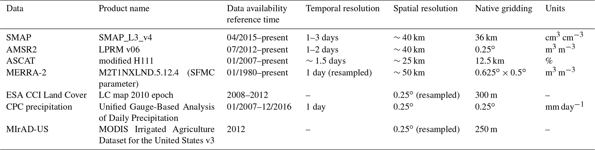
The data sources used in this study are summarized in Table 1.

3.1 Remotely sensed soil moisture

3.1.1 SMAP

The Soil Moisture Active Passive (SMAP) mission was launched in January 2015 and is the second mission exclusively designed for the retrieval of soil moisture together with freeze and/or thaw status (Entekhabi et al., 2010). After failure of its radar in July 2015, the radiometer continues to provide measurements in the L band (1.4 GHz) at a spatial resolution of approximately 40 km. Validation studies have shown that the radiometer meets the target retrieval accuracy of 0.04 m³ m⁻³ (unbiased RMSE, ubRMSE) over non-frozen land surfaces free of excessive snow, ice, mountainous terrain and dense vegetation coverage (Colliander et al., 2017). In general, the L band is expected to be more suitable for soil moisture retrieval, because it is less affected by vegetation and representative of a deeper soil layer than higher frequency C- or X-band retrievals (Entekhabi et al., 2010). SMAP obtains global coverage every 2–3 days and equatorial crossing times are 06:00 and 18:00 local solar time (LST) for the descending and ascending orbits, respectively. We used both ascending and descending orbit data covering the period of April 2015 to December 2016. We used the L3_SM_P V5 data product, which is sampled at 36 km resolution. In this product version, a water body correction and an improved soil temperature depth correction have been applied, which have respectively reduced anomalous soil moisture values near large water bodies and the dry bias with respect to the SMAP core validation sites (Jackson, 2018). In the case of overlapping orbits, we only used the descending (06:00 LST) overpass.

3.1.2 AMSR2

AMSR2 is a microwave radiometer on board the GCOM-W1 satellite and has provided measurements at 6.9 GHz (C band) and three higher frequencies up to 36.5 GHz (Ka band) since July 2012 (Imaoka et al., 2010). Daily ascending and descending overpasses are at 13:30 and 01:30 LST, respectively, achieving global coverage with a spatial resolution of about 40 km every 1–2 days. The VUA–NASA product used in this study is based on the Land Parameter Retrieval Model (LPRM) V6 algorithm, which simultaneously retrieves volumetric soil moisture and vegetation optical depth (VOD) from the observed brightness temperatures (Owe et al., 2008; der Schalie et al., 2016). LPRM is based on a radiative transfer equation and partitions the observation into its emission components from soil and vegetation based on the horizontal and vertical polarized brightness temperatures. Only observations from the descending orbits were used and, in addition, the retrievals were masked for high VOD values and radio frequency interference (RFI), spatially resampled to a regular 0.25^∘ grid and temporally centered at 00:00 UTC (Dorigo et al., 2017; Gruber et al., 2017; Liu et al., 2012).

3.1.3 ASCAT

The Advanced Scatterometer (ASCAT) on board the Meteorological Operational (Metop-A and B) satellites has been operational since October 2006 and is a real aperture radar instrument operating at C band (5.255 GHz) and VV polarization. Local equatorial crossing times are at 21:30 for the ascending overpass and at 09:30 for the descending overpass, and global coverage is achieved every 1–3 days depending on latitude. The TU Wien change detection algorithm (Wagner et al., 1999; Naeimi et al., 2009) is applied to the backscatter coefficients to create time series of relative surface soil moisture for the topmost centimeters of soil. This is accomplished by scaling each observation between reference values representing the historically lowest and highest observed backscatter values, respectively. Soil moisture is provided in degree of saturation (%) and ranges between 0 % (wilting point) and 100 % (soil saturation). It has a spatial resolution of 25 km and is made available on a discrete global grid (DGG) at a spatial sampling of 12.5 km. In this study, we used a modified version of the European Organisation for the Exploitation of Meteorological Satellites (EUMETSAT) Satellite Application Facility on Support to Operational Hydrology and Water (H-SAF) H111 soil moisture product. The modified version uses a dynamic correction which is expected to better account for inter-annual variability than the original H111 product (Hahn et al., 2017; Vreugdenhil et al., 2016).

3.2 MERRA-2 reanalysis soil moisture

The second Modern-Era Retrospective analysis for Research and Applications 2 (MERRA-2) (Bosilovich et al., 2016) is an atmospheric reanalysis product providing global, hourly fields of land surface and atmospheric conditions for 1980–present at a spatial resolution of $\mathrm{0.625}{}^{\circ }\times \mathrm{0.5}{}^{\circ }$. It assimilates atmospheric satellite observations using the Goddard Earth Observing System Model (GEOS-5). MERRA-2 uses an observation-based precipitation correction over land to fully correct modeled precipitation at latitudes $<\left|\mathrm{42.5}{}^{\circ }\right|$, with a linear tapering between $\left|\mathrm{42.5}{}^{\circ }\right|<\mathrm{latitude}<\left|\mathrm{62.5}{}^{\circ }\right|$, while no correction is applied at more northern and southern latitudes. The precipitation correction has significantly improved the soil moisture simulations with respect to its predecessor (Reichle et al., 2017a). The soil moisture simulations are representative of the first 5 cm of soil and are expressed in volumetric units (m³ m⁻³). We explicitly chose MERRA-2 soil moisture in favor of soil moisture from other global reanalysis data sets, because MERRA-2 does not assimilate surface humidity and surface temperature observations (Reichle et al., 2017c), which are directly impacted by irrigation (Wei et al., 2013; Tuinenburg and Vries, 2017). MERRA-2 surface soil moisture simulations were evaluated in Reichle et al. (2017b) with in situ soil moisture data from 320 sites. It was shown that the modeled estimates are biased by 0.053 m³ m⁻³, which is approximately in the order of the SMAP soil moisture retrieval target accuracy.

3.3 Ancillary data

Despite the drawbacks discussed in Sect. 1.2, the ESA CCI Land Cover data set (Bontemps et al., 2013) was used to create a cropland mask for the CONUS, because the classification of overall agricultural land cover (i.e., irrigated and rain-fed lands) proved to be accurate. For a more detailed analysis of the impact of precipitation, we used CPC Unified Gauge-Based Analysis of Daily Precipitation, which covers the CONUS at 0.25^∘ native resolution (Chen et al., 2008; Xie et al., 2010). Therefore, it is expected to provide more detailed information than the precipitation data set used to force MERRA-2 SM, which has a 0.5^∘ resolution.

3.4 Data preprocessing

As data from SMAP were only available from April 2015 onward, we extended the study period to include available AMSR2 and ASCAT data from 2013 to 2016. Hence, four growing seasons with varying climatic conditions were covered by the AMSR2 and ASCAT sensors and two growing seasons by SMAP. We assumed a general growing season for the entire CONUS from the start of April to the end of September. All data were spatially matched to a common 0.25^∘ regular grid using nearest-neighbor resampling. In order to constrain the analysis to areas where irrigation is feasible, we masked all pixels with < 5 % of fractional cropland area based on ESA CCI Land Cover for 2010 (Bontemps et al., 2013). Unreliable observations in the satellite data were masked, applying their respective quality flags for frozen soil, dense vegetation and radio frequency interference.

The spatial representativeness and observation depth slightly differ among the various remote sensing products and modeled soil moisture. MERRA-2 SM is simulated for a fixed 5 cm thick soil layer (Bosilovich et al., 2016) and thus shows more inertia to changes in the water balance (i.e., through precipitation) than the remotely sensing data. Besides, ASCAT is provided in a different unit than the other products. To account for these systematic differences between products, we applied a linear rescaling approach (Brocca et al., 2013), which forces the satellite soil moisture time series Θ^sat to have the same mean μ and standard deviation σ as the modeled soil moisture Θ^mod:

$$\begin{array}{}\text{(1)}& {\mathrm{\Theta }}_{\mathrm{rescaled}}^{\mathrm{sat}}={\displaystyle \frac{{\mathrm{\Theta }}^{\mathrm{sat}}-\mathit{\mu }\left({\mathrm{\Theta }}^{\mathrm{sat}}\right)}{\mathit{\sigma }\left({\mathrm{\Theta }}^{\mathrm{sat}}\right)}}\mathit{\sigma }\left({\mathrm{\Theta }}^{\mathrm{mod}}\right)+\mathit{\mu }\left({\mathrm{\Theta }}^{\mathrm{mod}}\right).\end{array}$$

It is likely that over irrigated areas μ(Θ^sat) increases during the respective irrigation period, which alters the scaling parameters. We expect that this should not affect the temporal evolution of changes in soil moisture. However, the influence of irrigation on the temporal variability of soil moisture (depending on the type of irrigation, general climate conditions, etc.) is a source of uncertainty. In particular over very dry regions, the model soil moisture may never reach saturation, while the remotely sensed soil moisture data do (due to irrigation). Since the variable of interest is irrigation amount, volumetric soil moisture in m³ m⁻³ is converted to the corresponding water column depth D_watertable (mm) by multiplying it with the depth of soil D_soil for which the soil moisture simulations are representative. Thus, for the layer 0–5 cm, for example, 0.3 m³ m⁻³ corresponds to a 15 mm water column covering the unit area of 1 m².

4 Methods

4.1 Theoretical foundation for retrieving irrigation water use from microwave remote sensing

Kumar et al. (2015) first proposed the idea of inferring irrigation from a positive bias between remotely sensed and modeled soil moisture, induced by seasonal water application during the dry season. This idea is based on two key assumptions: first, the satellite soil moisture products are sensitive to large-scale irrigation (as partly confirmed by Escorihuela and Quintana-Seguí, 2016; Lawston et al., 2017); and, second, the model does not account for irrigation, neither explicitly (i.e., in the formulation) nor implicitly through the assimilation of surface humidity or surface temperature observations, which are affected by irrigation (Wei et al., 2013). We build on these assumptions and introduce a new metric to estimate IWU from the difference between satellite-observed and modeled soil moisture. The soil water balance equations describing the respective change in soil moisture for each time step t (day) are described by

$$\begin{array}{}\text{(2)}& {\displaystyle \frac{d{\mathrm{\Theta }}^{\mathrm{sat}}}{\mathrm{d}t}}=P\left(t\right)+I\left(t\right)-\mathrm{ET}\left(t\right)-R\left(t\right)-\mathrm{\Delta }{S}_{\mathrm{rest}}\end{array}$$

for the satellite observations and

$$\begin{array}{}\text{(3)}& {\displaystyle \frac{\mathrm{d}{\mathrm{\Theta }}^{\mathrm{mod}}}{\mathrm{d}t}}=P\left(t\right)-\mathrm{ET}\left(t\right)-R\left(t\right)-\mathrm{\Delta }{S}_{\mathrm{rest}}\end{array}$$

for the model simulations. P (mm) is precipitation; I (mm) is irrigation; ET (mm) is evapotranspiration; and Θ^sat and Θ^mod (mm) are satellite and modeled surface soil moisture, respectively, converted to water column depth. ΔS_rest (m³ m⁻³) describes water storage changes below the surface layer, including drainage. Subtracting Eq. (3) from Eq. (2) yields

$$\begin{array}{}\text{(4)}& I\left(t\right)={\displaystyle \frac{\mathrm{d}{\mathrm{\Theta }}^{\mathrm{sat}}}{\mathrm{d}t}}-{\displaystyle \frac{\mathrm{d}{\mathrm{\Theta }}^{\mathrm{mod}}}{\mathrm{d}t}}.\end{array}$$

Hence, estimating irrigation from differences between the temporal variations of satellite and model SM is theoretically feasible.

4.2 Deriving irrigation water use

We define an irrigation event as a simultaneous increase in satellite soil moisture $\left(\frac{\mathrm{d}{\mathrm{\Theta }}^{\mathrm{sat}}}{\mathrm{d}t}>\mathrm{0}\right)$ and a decrease or stagnation in model soil moisture $\left(\frac{\mathrm{d}{\mathrm{\Theta }}^{\mathrm{mod}}}{\mathrm{d}t}\le \mathrm{0}\right)$. This means that rainfall did not cause the satellite-observed increase in soil moisture, which over agricultural land was very likely a result of irrigation. For each event, the amount of irrigation water leading to the increase is derived as the difference $\frac{\mathrm{d}{\mathrm{\Theta }}^{\mathrm{sat}}}{\mathrm{d}t}-\frac{\mathrm{d}{\mathrm{\Theta }}^{\mathrm{mod}}}{\mathrm{d}t}$, if the change in satellite is significant (i.e., above the noise level). The latter is accounted for by applying a threshold of relative soil moisture change thresh_Θ (see Sect. 4.3 and Appendix A). We then calculate seasonal irrigation water use (IWU) summing up the approximated difference quotients over the growing season period:

$$\begin{array}{}\text{(5)}& {\displaystyle }\mathrm{IWU}=\underset{i_{\mathrm{SOS}}}{\overset{i_{\mathrm{EOS}}}{\int }}(\mathrm{d}{\mathrm{\Theta }}_i^{\mathrm{sat}}-\mathrm{d}{\mathrm{\Theta }}_i^{\mathrm{mod}})\mathrm{d}t\approx \sum _{i=\mathrm{SOS}}^{\mathrm{EOS}}\mathrm{\Delta }{\mathrm{\Theta }}_i^{\text{sat-mod}},\end{array}$$

where

$$\mathrm{\Delta }{\mathrm{\Theta }}_i^{\text{sat-mod}}=\left\{\begin{array}{ll}\mathrm{\Delta }{\mathrm{\Theta }}_i^{\mathrm{sat}}-\mathrm{\Delta }{\mathrm{\Theta }}_i^{\mathrm{mod}},& \mathrm{if}\mathrm{\Delta }{\mathrm{\Theta }}_i^{\mathrm{sat}}\ge {\mathrm{\Theta }}_{\mathrm{thresh}}\\ \mathrm{0},& \mathrm{otherwise}\end{array}\right.$$

and with

$$\begin{array}{ll}{\displaystyle }& {\displaystyle }\mathrm{\Delta }{\mathrm{\Theta }}_i^{\mathrm{sat}}={\mathrm{\Theta }}_i^{\mathrm{sat}}-{\mathrm{\Theta }}_{i-n}^{\mathrm{sat}}\text{, }\\ {\displaystyle }& {\displaystyle }\mathrm{\Delta }{\mathrm{\Theta }}_i^{\mathrm{mod}}={\mathrm{\Theta }}_i^{\mathrm{mod}}-{\mathrm{\Theta }}_{i-n}^{\mathrm{mod}}.\end{array}$$

IWU is the accumulated irrigation water use from the start (i_SOS) until the end of the growing season (i_EOS). According to the crop calendars provided by Portmann et al. (2010) and the USDA planting and harvesting dates handbook (NASS, 2010) the period 1 April–30 September generally covers the growing season of most crops receiving irrigation water in the CONUS. ${\mathrm{\Theta }}_i^{\mathrm{sat}}$ and ${\mathrm{\Theta }}_i^{\mathrm{mod}}$ are satellite and model SM on day i, thresh_Θ denotes the relative soil moisture threshold, and ${\mathrm{\Theta }}_{i-n}^{\mathrm{sat}}$ and ${\mathrm{\Theta }}_{i-n}^{\mathrm{mod}}$ are the last available soil moisture observations with a data gap of n days. If an irrigation event is detected during an observation gap of > 4 days, we check if there has been a significant increase in the model soil moisture (e.g., due to rainfall) within that period. When more than one significantly positive model slope (or precipitation events) occurs during the gap period, we cannot say for sure if the observed increase in soil moisture was due to irrigation or precipitation and therefore conservatively disregard the potential irrigation event.

4.3 Masking spurious irrigation detections

It is essential to differentiate between irrigation signals and high-frequency noise in the satellite data. For this purpose, we apply a threshold thresh_Θ to the relative changes in satellite soil moisture similar to the approach applied by Dorigo et al. (2013) to detect spurious in situ data:

$$\begin{array}{}\text{(6)}& {\displaystyle \frac{{\mathrm{\Theta }}_t^{\mathrm{sat}}-{\mathrm{\Theta }}_{t-n}^{\mathrm{sat}}}{{\mathrm{\Theta }}_{t-n}^{\mathrm{sat}}}}\ge \mathrm{0.12}\equiv {\mathrm{thresh}}_{\mathrm{\Theta }}.\end{array}$$

Based on an extensive sensitivity analysis (Appendix A) we concluded that a threshold of thresh_Θ≡0.12 is an appropriate generic choice for the whole CONUS.

Potential errors may arise when the model forcing misses or creates false rainfall events. In addition, because of differences in timing of the estimates and differences in represented soil depth between remotely sensed and modeled soil moisture, their response to precipitation events may differ as well. This may lead to spurious irrigation events when irrigation is estimated on days with rainfall. Therefore, we use information from an additional CPC precipitation data set at 0.25^∘ resolution, thus providing an approximately 4× higher spatial resolution than the rainfall product used to force MERRA-2 (see Sect. 3.2). This allows us to make a more educated guess when evaluating if the observations and/or model estimates are affected by rainfall. Furthermore, if a potential irrigation signal coincides with preceding rainfall we assume that irrigation is unlikely and disregard the event. In some extreme cases, capillary rise from deeper soil layers or run-on can wet the top soil. Theoretically, these conditions are reflected by the satellite soil moisture retrievals but are absent in the model soil moisture simulations (i.e., if such effects are not accounted for in the soil hydrology formulation of the LSM, McColl et al., 2017). However, at the large spatial scales represented by the employed satellite (approximately 25 km) and model soil moisture products (approximately 50 km), very few pixels are expected to show positive $\mathrm{\Delta }{\mathrm{\Theta }}_i^{\mathrm{sat}}$ or $\mathrm{\Delta }{\mathrm{\Theta }}_i^{\mathrm{mod}}$ in the absence of precipitation or irrigation. Another impact concerns mismatches between the ancillary data used to force the model and parametrize the respective satellite soil moisture retrieval algorithms, such as land cover and soil parameters. By rescaling to the model dynamic soil moisture range, we implicitly account for mismatches in soil parameters. However, addressing potential mismatches in land cover was out of the scope of this paper and thus represents an intrinsic limitation of the method.

5 Results and discussion

5.1 Growing season correlations between satellite and model soil moisture

To investigate the potential detectability of IWU, we investigated the correlation between satellite and modeled soil moisture during the growing season (Fig. 3). We computed the correlation separately for dry (precipitation =0; ${\stackrel{\mathrm{‾}}{r}}_{\mathrm{dry}}$) and wet conditions (precipitation > 0; ${\stackrel{\mathrm{‾}}{r}}_{\mathrm{wet}}$). If ${\stackrel{\mathrm{‾}}{r}}_{\mathrm{dry}}$ is low or negative over agricultural areas which are known to be irrigated (as inferred from the MIrAD-US product) while ${\stackrel{\mathrm{‾}}{r}}_{\mathrm{wet}}$ is strongly positive, this is a strong indication of irrigation (also see Fig. A2, where the absolute differences between the mean correlations for wet and dry periods $|r_{\mathrm{wet}}-r_{\mathrm{dry}}|$ are shown).

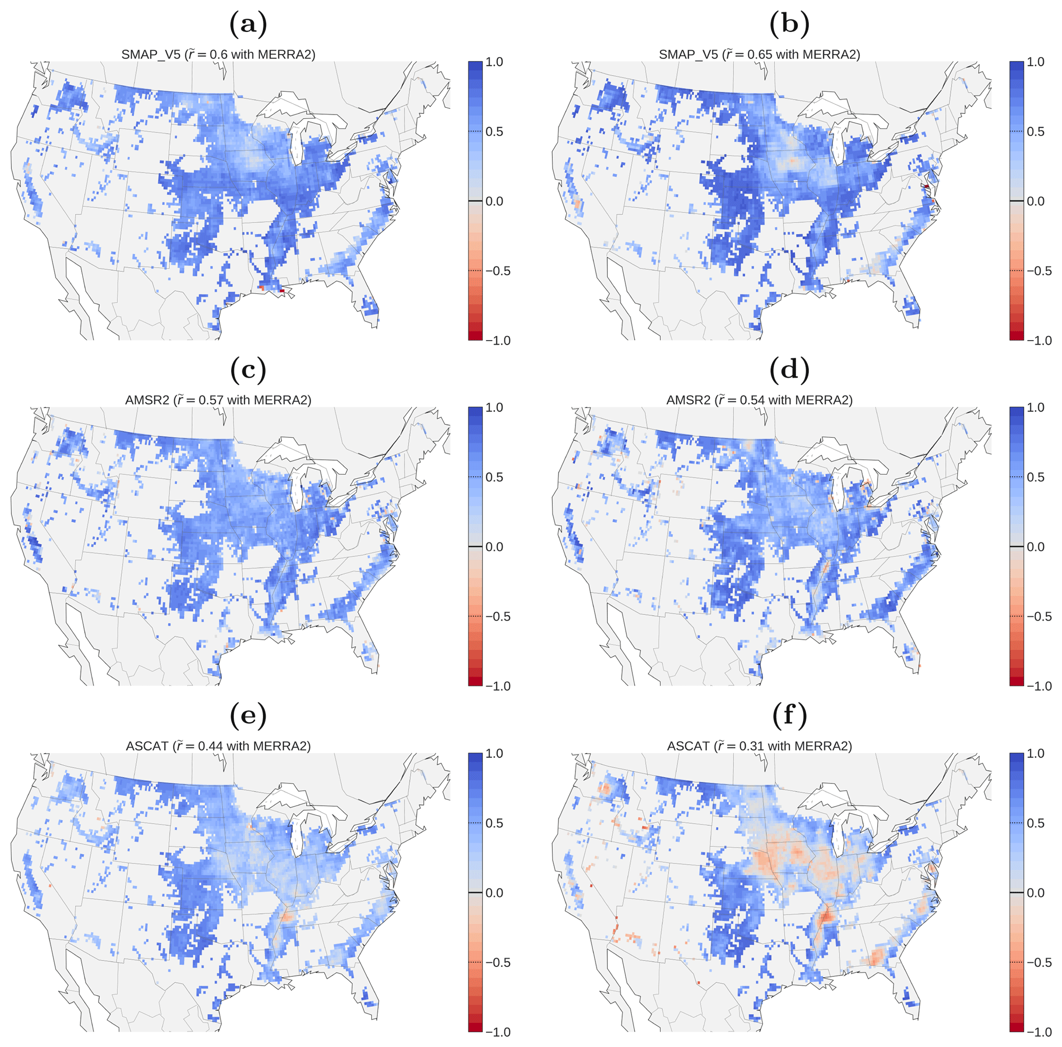
Figure 3 Mean correlation $\stackrel{\mathrm{‾}}{r}$ between the daily time series of each satellite soil moisture product (SMAP, AMSR2 and ASCAT) and MERRA-2 soil moisture separated for wet periods (left column; precipitation PCP >0) and dry periods (right column; PCP =0) during the growing season. Correlations were calculated over agricultural areas only.

Over non-agricultural land cover, low growing season correlations between SMAP and MERRA-2 soil moisture are observed over the densely vegetated south- and northeastern US, as well as over parts of the arid southwest (Fig. 3a, b). AMSR2 exhibits low correlations in coastal areas, complex terrain and over dense vegetation cover (Fig. 3c, d). ASCAT shows negative correlations against MERRA-2 over the arid southwestern deserts and the densely vegetated coastal northwest and southeast (Fig. 3e, f). Overall, for each satellite–model pair there is a clear reduction of ${\stackrel{\mathrm{‾}}{r}}_{\mathrm{dry}}$ with respect to ${\stackrel{\mathrm{‾}}{r}}_{\mathrm{wet}}$ over several irrigation hot spots within the CONUS.

5.1.1 Central Valley

Over the Central Valley, SMAP shows moderate to high ${\stackrel{\mathrm{‾}}{r}}_{\mathrm{wet}}$ with MERRA-2, except for the Sacramento Valley in northern California. In contrast, ${\stackrel{\mathrm{‾}}{r}}_{\mathrm{dry}}$ is moderately to strongly negative over the southern San Joaquin Valley, which indicates that an irrigation signal is indeed observed by the satellite sensor. The fact that ${\stackrel{\mathrm{‾}}{r}}_{\mathrm{dry}}$ is comparable to, if not higher than, ${\stackrel{\mathrm{‾}}{r}}_{\mathrm{wet}}$ over the Sacramento Valley should be attributed to the special characteristics of the prevalent rice irrigation. In the Sacramento Valley, a permanent flood of 10–15 cm is usually maintained during the whole growing season before fields are drained in preparation for harvest (Linquist et al., 2015). Hence, irrigation water remains observable during both wet- and dry periods of the growing season, and the impact of irrigation on $\stackrel{\mathrm{‾}}{r}$ actually increases for the wet period with respect to the dry period. In contrast, ASCAT exhibits high correlations with MERRA-2 in this region. During the early phenological growth phase of rice, this observation can be attributed to specular reflection of the radar signal from the flood water surface, given that wind speeds do not significantly affect the water's surface roughness (Nguyen et al., 2015). By the time the rice stems start to break through the water surface the now elongated rice stems are known to act as double-bounce reflectors, which commonly results in an enhanced backscatter signal that can be observed until field drainage in late summer (Le Toan et al., 1997; Nguyen et al., 2016) (see ASCAT soil moisture time series in Fig. 5b). Both SMAP and ASCAT show moderate to high negative correlations against MERRA-2 in the heavily irrigated San Joaquin Valley. Concerning AMSR2 SM there is no clear pattern of discrepancy between ${\stackrel{\mathrm{‾}}{r}}_{\mathrm{wet}}$ and ${\stackrel{\mathrm{‾}}{r}}_{\mathrm{dry}}$ in the Central Valley.

5.1.2 Snake River Plain

Over the Snake River Plain, ASCAT has a clear signal that could be attributed to irrigation. Particularly in the central and westernmost areas along the Snake River, ${\stackrel{\mathrm{‾}}{r}}_{\mathrm{dry}}$ depicts a strong negative correlation with MERRA-2, while ${\stackrel{\mathrm{‾}}{r}}_{\mathrm{wet}}$ is moderately positive. Moderately negative ${\stackrel{\mathrm{‾}}{r}}_{\mathrm{dry}}$ obtained for SMAP shows a good alignment with areas known to be irrigated in the Snake River Plain. Although the correlation is less negative than for ASCAT, the spatial pattern is resembled more clearly. Here, AMSR2 shows slightly more negative ${\stackrel{\mathrm{‾}}{r}}_{\mathrm{dry}}$ than ${\stackrel{\mathrm{‾}}{r}}_{\mathrm{wet}}$ over agricultural land cover, but the spatial pattern appears to be less reliable than for the other satellite products.

5.1.3 High Plains

The ASCAT product is the only one to show a distinct pattern of negative correlation over the irrigated part of the Nebraska Plains. While ${\stackrel{\mathrm{‾}}{r}}_{\mathrm{wet}}$ shows weak positive correlations, ${\stackrel{\mathrm{‾}}{r}}_{\mathrm{dry}}$ reveals strong negative $\stackrel{\mathrm{‾}}{r}$, suggesting that an irrigation signal is entailed in the ASCAT signal. However, this pattern cannot be reliably attributed to irrigation practices as ASCAT shows low correlations over the entire Corn Belt region, where agriculture is generally known to be rain-fed (see Fig. 2). Vegetation scattering effects from the corn canopies are a plausible explanation for the observed deviation. As the corn plants reach their maximum height (up to approximately 3 m) towards the end of the growing season, the C-band backscatter signal will increasingly be composed of canopy backscatter and canopy-soil double-bounce reflections, while sensitivity to actual soil moisture decreases (Daughtry et al., 1991; Joseph et al., 2010).

5.1.4 Mississippi Floodplain

Lastly, all products show low $\stackrel{\mathrm{‾}}{r}$ values over the Mississippi Floodplain, although with varying magnitudes. In this region, ASCAT shows the lowest negative correlation, followed by AMSR2 and SMAP. Moreover, for all SM products ${\stackrel{\mathrm{‾}}{r}}_{\mathrm{dry}}$ is lower than ${\stackrel{\mathrm{‾}}{r}}_{\mathrm{wet}}$.

5.1.5 Other regions

Figure 3 also reveals that strong negative ${\stackrel{\mathrm{‾}}{r}}_{\mathrm{dry}}$ (in combination with moderately high ${\stackrel{\mathrm{‾}}{r}}_{\mathrm{wet}}$) based on ASCAT aligns well with areas known to be irrigated over the Columbia River basin, Washington. As the ASCAT soil moisture product has a significantly higher nominal spatial resolution than the passive products, we hypothesize that in this region it is the only sensor to resolve the irrigation practices. Correlations based on SMAP loosely agree with this pattern and AMSR2 only has few valid observations over this region. In addition, both ASCAT and SMAP have patterns of ${\stackrel{\mathrm{‾}}{r}}_{\mathrm{dry}}$ < ${\stackrel{\mathrm{‾}}{r}}_{\mathrm{wet}}$ over an irrigated region in southwestern Georgia. In contrast, AMSR2 shows moderately high positive $\stackrel{\mathrm{‾}}{r}$ over this region.

To determine the sensitivity of the growing season correlation $\stackrel{\mathrm{‾}}{r}$ between satellite and model soil moisture to variations in fractional irrigated area within a pixel, we examined their relationship with irrigation intensities derived from the MIrAD-US irrigated area data set (Pervez and Brown, 2010). However, no evidence of a negative linear relationship between the two variables was found (not shown), as at low irrigation fractions $\stackrel{\mathrm{‾}}{r}$ is mostly dominated by effects originating from the remaining land cover types. Overall, the results obtained by separately analyzing the spatial patterns of ${\stackrel{\mathrm{‾}}{r}}_{\mathrm{dry}}$ and ${\stackrel{\mathrm{‾}}{r}}_{\mathrm{wet}}$ between satellite and model soil moisture largely support the hypothesis that, over areas known to be irrigated, the remotely sensed soil moisture signal deviates from modeled soil moisture, given that the model does not explicitly account for irrigation (which is the case for MERRA-2). Hence, the overall hypothesis of this study, which is that IWU can be inferred from differences between the temporal variations of the remotely sensed and modeled soil moisture, is corroborated.

5.2 Spatial patterns of estimated irrigation water use

Spatial plots of mean annual estimated irrigation water use $\stackrel{\mathrm{‾}}{\mathrm{IWU}}$ (i.e., averaged over the study period of 2013–2016) (Fig. 4a–c) suggest that all satellite products are able to identify the extensive irrigation applied in the California Central Valley. Here, SMAP-derived $\stackrel{\mathrm{‾}}{\mathrm{IWU}}$ clearly resembles the irrigation patterns of the MIrAD-US data set in the northern Sacramento Valley and southern San Joaquin Valley (Fig. 2). The AMSR2- and ASCAT-derived $\stackrel{\mathrm{‾}}{\mathrm{IWU}}$ are generally higher than SMAP and extend throughout the whole California Central Valley. Although small in magnitude, the $\stackrel{\mathrm{‾}}{\mathrm{IWU}}$ pattern derived from ASCAT over the central Snake River Plain is spatially distinct. Similarly, AMSR2 shows a clear signal over the western to central Snake River Plain. Concerning the Nebraska Plains, only AMSR2 $\stackrel{\mathrm{‾}}{\mathrm{IWU}}$ shows patterns that agree with MIrAD-US. Over the Mississippi Floodplain, ASCAT shows the highest $\stackrel{\mathrm{‾}}{\mathrm{IWU}}$, followed by AMSR2.

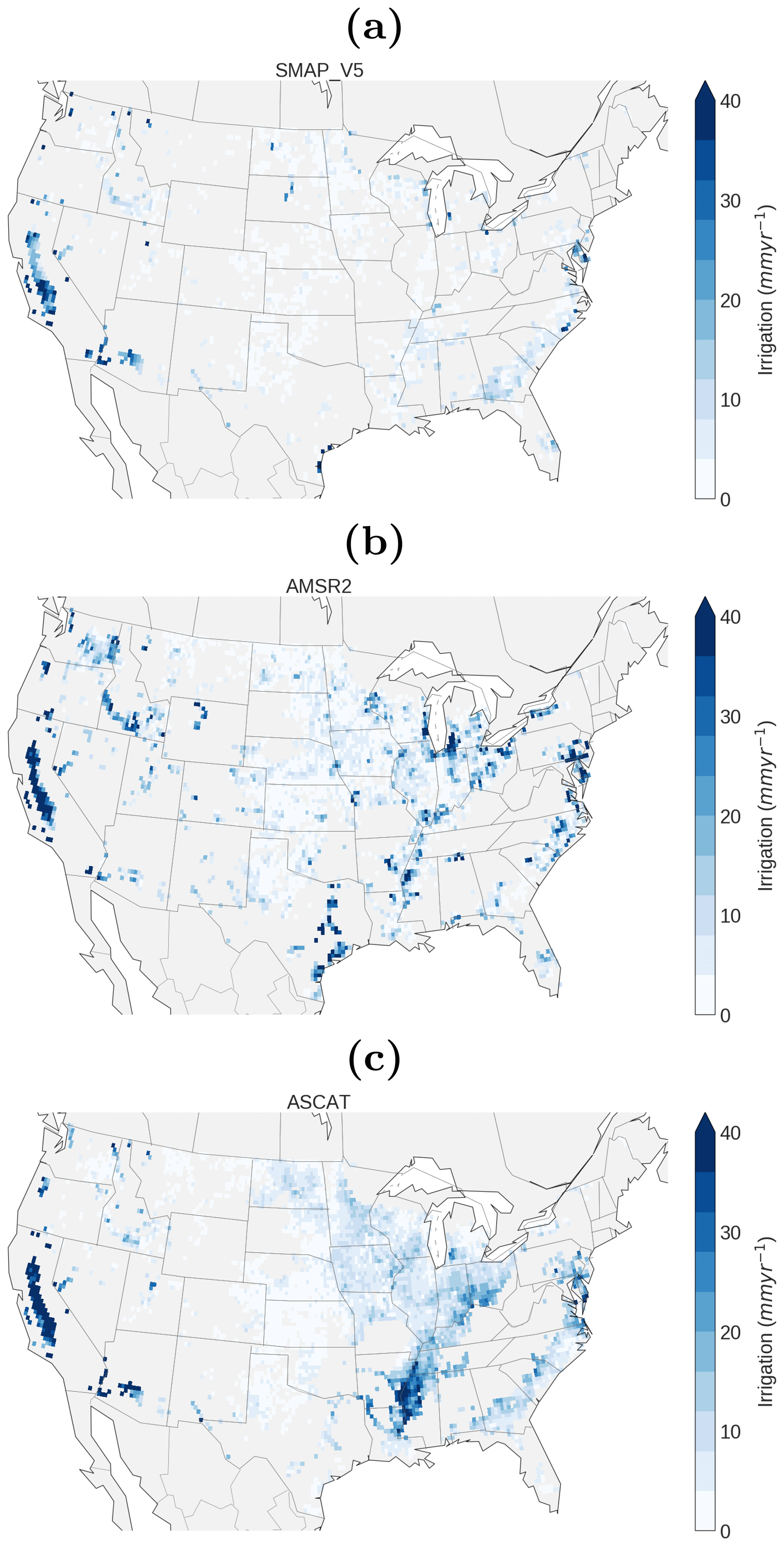
Figure 4 Mean annual irrigation water use ${\stackrel{\mathrm{‾}}{\mathrm{IWU}}}_{\mathrm{A}}$ derived from SMAP (a), AMSR2 (b), and ASCAT (c) SM in combination with modeled SM from MERRA-2. All pixels with a cropland fraction of <5 % (as inferred from the CCI Land Cover product) were excluded from the analysis. Note that for SMAP the climatologies represent the growing season mean of 2015 and 2016, while for AMSR2 and ASCAT the estimates are derived from 4 years of data covering the period of 2013–2016.

ASCAT-derived $\stackrel{\mathrm{‾}}{\mathrm{IWU}}$ seems to be affected by vegetation effects in the Corn Belt region and in the southeastern US. For all sensors, the method fails to detect $\stackrel{\mathrm{‾}}{\mathrm{IWU}}$ in many irrigated areas, especially those along the High Plains aquifer (Nebraska, Kansas, Texas), which extends from the northern to the southern central US. A plausible explanation for missing these areas is that many farmers in these regions practice supplemental irrigation, thus resulting in a less distinguishable irrigation signal. In addition, the center pivot irrigation systems, which are mainly used in this region, have much higher water application efficiencies compared to the flood and furrow irrigation systems used in the Sacramento Valley and Mississippi Floodplain (see Fig. A1). Rainfall seasonality is another potential reason for the underestimation in the central U.S, where the climate transitions from arid in the west to humid in the east. To investigate its impact, we plotted the average number of days per growing season where IWU >0 (Fig. A3), which sums up to the number of days that went into the $\stackrel{\mathrm{‾}}{\mathrm{IWU}}$ estimates shown in Fig. 4. It can be seen that for SMAP-based IWU, a significant number of days with irrigation (mean count) only is detected in the arid west and southwest. For AMSR2, the mean counts are highest in California, although counts in the range of 20–30 occur in the Snake River Valley, Mississippi Floodplain and other agricultural regions. In agreement with the passive products, mean counts for ASCAT are highest in California and southwestern states. There also is a clear pattern in the Mississippi Valley and along the southeastern states.

Furthermore, the chosen global threshold of thresh_Θ=12 % also masks irrigation signals in regions where the noise level of the satellite soil moisture retrievals is rather low (see Sect. A2). Thus, a more site-specific threshold at each pixel might lead to an improved detectability of irrigation events.

5.3 Temporal behavior of soil moisture and IWU and in the four focus regions

For a more detailed analysis on the impact of climate, crop type and irrigation practice on the method performance, we compared remotely sensed and modeled soil moisture time series and monthly IWU estimates at an irrigated (green crosses in Fig. 2) and a non-irrigated pixel (orange crosses in Fig. 2) in the four focus areas (Fig. 5).

Figure 5 Comparison of satellite and model SM time series at irrigated (top two sub-panels) and non-irrigated pixels (bottom two sub-panels) in five regions (Fig. 5a–e). Daily CPC precipitation is plotted in grey, while blue and orange shadings in the top sub-panels reflect growing seasons with positive and negative rainfall anomalies, respectively. The second and fourth sub-panels show the estimated monthly irrigation water use (${\stackrel{\mathrm{‾}}{\mathrm{IWU}}}_{\mathrm{M}}$) obtained for each satellite–model pair for the irrigated and non-irrigated pixels, respectively (non-growing season periods have been masked).

5.3.1 Central Valley

At the irrigated pixel in the San Joaquin Valley, the impact of irrigation on the remotely sensed soil moisture signal is evident (top panel in Fig. 5a). While MERRA-2 soil moisture decline in the irrigated and non-irrigated pixels reflects the absence of precipitation, typically from mid-May until mid-October, ASCAT and SMAP soil moisture in the irrigated pixel start to increase in June until reaching their maximum in July–August and gradually declining towards the end of the growing season. In contrast, remotely sensed soil moisture in the adjacent non-irrigated pixel (bottom panel) remains close to zero throughout the growing season. The temporal behavior of SMAP at the irrigated pixel location was extensively evaluated by Lawston et al. (2017), who showed that SMAP soil moisture correctly reflects the onset of flood irrigation, the dry-down associated with plants breaking through the water surface (which attenuates the SM signal) and lastly field drainage. Even though Lawston et al. (2017) used the enhanced 9 km sampling SMAP product, we find very comparable temporal characteristics for the native 36 km resolution product (Fig. 5b). ASCAT soil moisture seems to be impacted by specular reflection of the active radar signal from the flooded rice fields, leading to very low backscatter and, hence, soil moisture values. As a result, particularly during the 2013 growing season, ASCAT soil moisture remains at or very close to its minimum early in the growing season. ASCAT soil moisture starts to increase in early to mid-July when the rice starts to break out of the water. Initially, the increase is primarily the result of double-bounce effects from the rice canopies, while at later growth stages this turns into volume scattering (Nguyen et al., 2015). Of the three products, ASCAT soil moisture is the last to reach its growing season maximum between mid- and late August, followed by a decrease throughout September. At the irrigated pixel, AMSR2 soil moisture shows large fluctuations during the growing season, while at the non-irrigated pixel it has few valid observations, which makes it difficult to compare both pixels. AMSR2 soil moisture shows similar characteristics with respect to SMAP and is able to sense the onset of flood irrigation but reaches saturation a few weeks earlier and already starts to dry down before SMAP reaches its soil moisture maximum. Moreover, after reaching a minimum in late July to early August, AMSR2 soil moisture starts to increase again.

Comparing the estimated monthly IWU (bottom sub-panels) at the adjacent irrigated and non-irrigated pixels suggests that the method is skillful in detecting irrigation from all considered sensors, especially during the comparatively dry years of 2013 and 2014, when a prolonged drought affected the State of California. AMSR2 provides highest IWU estimates, possibly due to the high noise levels in the soil moisture data. In general, a spurious irrigation signal remains at the non-irrigated pixel, which may be due to noise in the satellite soil moisture retrievals. At the non-irrigated pixel, ASCAT- and AMSR2-based IWU retrievals seem to be more affected by noise than SMAP. The 2015 growing season was unusually wet, which at the non-irrigated pixel resulted in the spurious detection of irrigation for all satellite products. Generally, SMAP and ASCAT products are especially skillful in detecting the seasonality of irrigation over the San Joaquin Valley.

5.3.2 Snake River Plain

At Snake River Plain, all satellite soil moisture products show a clear irrigation signal at the irrigated pixel (Fig. 5c), which is not visible in the non-irrigated pixel. Consequently, considerable IWU is estimated for the irrigated pixel, while for ASCAT and SMAP the estimated IWU at the non-irrigated pixel is close to zero. AMSR2 soil moisture retrievals are noisier, which results in the detection of some spurious irrigation at the non-irrigated pixel, although significantly smaller than at the irrigated pixel. We argue that the higher spatial sampling of the employed ASCAT data is advantageous for IWU estimation, as the irrigated area within the Snake River Plain is quite narrow.

5.3.3 High Plains

ASCAT soil moisture content is higher than MERRA-2 during the drier periods of the growing season, indicating sensitivity to the typically employed supplemental irrigation (Fig. 5d). However, the relative changes in ASCAT soil moisture are < 12 % and therefore do not qualify as rigorous irrigation events based on our methodology. AMSR2 provides the largest derived IWU at the irrigated pixel but is also affected by noise at the non-irrigated pixel. In this area, the influence of irrigation on the remotely sensed soil moisture signal is much more subtle, if significant at all. This can be attributed to two factors. First, due to the abundant rainfall during the growing season only supplemental irrigation is applied in this area. Second, center pivot irrigation systems usually have much higher application efficiencies (75 %–95 %) than gravity irrigation systems (40 %–80 %). Therefore, less water needs to be applied to achieve comparable plant growth, rendering a less distinct irrigation signal in the soil moisture product.

5.3.4 Mississippi Floodplain

The difference in soil moisture behavior between the irrigated and non-irrigated pixel is much more pronounced for AMSR2 than for the other satellite products (Fig. 5e). This is also reflected by AMSR2-derived IWU at the irrigated pixel, which agrees well with the expected seasonality of irrigation, which peaks in August. At the same time AMSR2-based IWU estimates are close to zero at the non-irrigated pixel. ASCAT soil moisture shows a similar seasonality at the irrigated pixel but is more affected by noise at the non-irrigated pixel. SMAP soil moisture sustains saturation throughout the first half of the growing season, which could either be caused by flood irrigation for rice or point at a problem in the soil moisture retrieval algorithm. At least for AMSR2, IWU shows a meaningful derived seasonality.

Figure 6 Comparison of estimated mean annual irrigation water use and reported irrigation water withdrawals. For each satellite–model pair, observed ${\stackrel{\mathrm{‾}}{\mathrm{IWU}}}_{\mathrm{A}}$ was aggregated at the state level. Reported irrigation withdrawals were taken from the 2013 FRIS report and only reflect volumes applied in open fields (e.g., excluding crops grown and irrigated in greenhouses). The data are presented in logarithmic units to reflect both small and large water volumes. Note that the names of the 10 states accounting for the highest irrigation water withdrawals are annotated. R, RMSE and bias between observed and reported estimates are shown in the bottom right of each subplot.

5.4 Evaluation of estimated irrigation water use against state-level reference water withdrawals

We evaluated the agreement between mean IWU, $\stackrel{\mathrm{‾}}{\mathrm{IWU}}$, aggregated for each satellite–model pair to the state level, and reported irrigation water withdrawals from the 2013 FRIS (USDA, 2013) (IWW_FRI). The median correlation R values for SMAP-, AMSR2- and ASCAT-based $\stackrel{\mathrm{‾}}{\mathrm{IWU}}$ and IWW_FRIS are 0.80, 0.56 and 0.36, respectively (Fig. 6). For all satellite data sets, California is correctly identified as the largest consumer of irrigation water, which indicates the overall potential of coarse-resolution microwave soil moisture data in estimating IWU. However, the root-mean-square difference (RMSD) and bias between observed $\stackrel{\mathrm{‾}}{\mathrm{IWU}}$ and IWW_FRIS indicate a clear underestimation. The lowest RMSD of 5.21 km³ was found for AMSR2, but values for SMAP and ASCAT are quite similar. ASCAT has the lowest bias (−2.29 km³), but the bias based on the other products is similar. We further discuss the potential reasons for the generally large biases observed in Sect. 5.6. On average, $\stackrel{\mathrm{‾}}{\mathrm{IWU}}$ based on SMAP provides the closest similarity with IWW_FRI.

5.5 Evaluating irrigated area estimates with the MIrAD-US data set

We compared spatial patterns of total mean $\stackrel{\mathrm{‾}}{\mathrm{IWU}}$ estimates with the MIrAD-US data set at 0.25^∘ resolution. In order to compute a confusion matrix, we converted the continuous ranges of the two data sets into binary representations of irrigated areas. For MIrAD-US, this was accomplished by labeling only areas with >= 5 % irrigation fraction as irrigated. Estimated $\stackrel{\mathrm{‾}}{\mathrm{IWU}}$ was converted in a similar way by considering only pixels where $\stackrel{\mathrm{‾}}{\mathrm{IWU}}\ge X$ as irrigated, where X (mm) is a binarization threshold. To compare irrigation estimated from each satellite–model pair with MIrAD-US, we computed the error of omission (EoO), the error of commission (EoC), the overall accuracy (OA) and Cohen's kappa (κ), which is a measure of how the classification results compare to values assigned by chance (Table 2). The binarization threshold X was determined by maximizing κ for each satellite–model pair and focus region, respectively, as well as for the whole CONUS (see Fig. A5).

Table 2 Accuracy assessment of irrigated area estimates. For each satellite–model combination a confusion matrix between observed ${\stackrel{\mathrm{‾}}{\mathrm{IWU}}}_A$ and reference irrigated area from the spatially aggregated 2012 MIrAD-US data set was computed after converting the continuous data to a binary representation. Specifically, pixels with observed ${\stackrel{\mathrm{‾}}{\mathrm{IWU}}}_A\ge X$ mm and reported A_{crop-fraction}≥5 % were respectively assigned to the irrigated classes. The binarization thresholds X were found by maximizing the respective kappa scores for each satellite–model combination within each region (see Fig. A5). Results are shown for the four states selected in the regional analysis and the whole CONUS. Italics indicate the best scores within each region, while bold scores show the overall best.

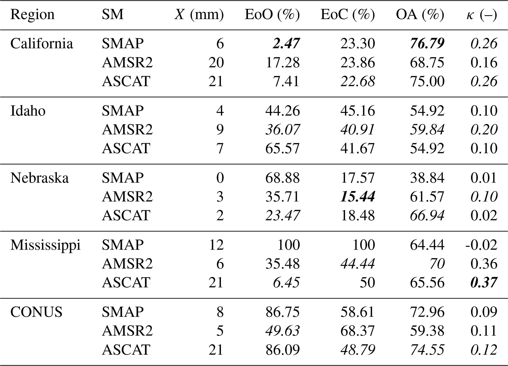
In California, irrigated area estimates based on $\stackrel{\mathrm{‾}}{\mathrm{IWU}}$ show very good agreement with MIrAD-US. SMAP-based irrigated areas provides the highest scores for all metrics: the overall accuracy is 76.79 %. A commission error (EoC) of 23.30 % in combination with an omission error (EoO) of 2.47 % indicates that we somewhat overestimate the reference, and a kappa score of κ=0.33 illustrates a fair agreement. ASCAT has a similar performance but shows a slightly higher overestimation (EoC =22.68 %), thus resulting in a lower overall accuracy and κ score. In California, AMSR2 performs worst but still shows an acceptable overall accuracy of 68.75 %. In Idaho, of all satellite products AMSR2 shows the highest agreement with the reference (OA =59.84 %), but EoC and EoO are equally high at approximately 40 %, indicating a moderate amount of confusion in the classification. As a result of a strong under-classification, in Nebraska there is hardly any agreement between IWU-based and MIrAD-US irrigated area. Over the Mississippi Floodplain, AMSR2- and ASCAT-based IWU shows moderately good agreement with the reference data (OA ≈70 %, κ>0.30). We argue that, due to the previously observed problems regarding the representation of soil saturation, SMAP soil moisture data are unreliable in this region. ASCAT-based IWU depicts a high overestimation (EoC =50 %) while SMAP-based IWU does not classify any irrigated areas at all (EoO =100 %). For CONUS as a whole, ASCAT and SMAP depict the best spatial agreement with MIrAD-US irrigated area, which is reflected by an overall accuracy of 74.55 % and 72.96 %, respectively. However, SMAP fails to correctly classify approximately 90 % of areas irrigated according to the MIrAD-US. AMSR2 shows an agreement of OA =59.38 % and misses fewer pixels than ASCAT and SMAP (EoO =49.63 %) but in contrast shows a higher overestimation (EoC =68.37 %).

The results obtained for California are encouraging and emphasize the potential of coarse-scale microwave soil moisture retrievals in correctly detecting the spatial patterns of irrigation. However, consistent with the findings of estimated irrigation volumes, irrigated area estimates reflect a general pattern of underestimation with respect to the MIrAD-US data set. The results further indicate that in areas such as Nebraska, where the climate is semi-humid in large parts of the state and irrigation is mostly supplementary, the method fails in detecting the irrigation signal.

5.6 Sensitivity of microwave soil moisture products to irrigation

By qualitatively examining the obtained results, we find that the sensitivity of the employed microwave soil moisture retrievals to irrigation and the performance with respect to reported irrigation data particularly depend on the following factors.

1. Spatial resolution of the microwave soil moisture products and topography. Likely, the largest restriction is the coarse scale of the satellite soil moisture retrievals with respect to the average field size. For instance, the area irrigated by a typical center pivot system (i.e., 500 m) is approximately 50 ha, which only accounts for approximately 0.0003 % of the satellite footprint area. Thus, around 3200 center pivot systems are needed to create a uniformly irrigated area covering the remotely sensed footprint. In the CONUS, areas with large irrigation fractions exist in the eastern half of the country, but irrigation in the arid western half is a lot more heterogeneous. In these areas, irrigation usually mainly depends on surface water supply and is therefore reserved to narrow river valleys such as the Colorado River valley. As a consequence, coarse-scale microwave soil moisture products may be insensitive to locally significant (but insignificant with respect to the scale of the satellite footprint) irrigation due to the small scale of the irrigation practices and surrounding complex topography (e.g., mountains, valley transitions, water bodies). As discussed in Sect. 5.1, in the Columbia River basin correlation patterns based on the ASCAT soil moisture product (which has a significantly higher nominal spatial resolution than the passive products) matched very well with the MIrAD-US product. An investigation of time series over this region (not shown) revealed that, there, ASCAT soil moisture carries a distinct seasonal irrigation signal. The reason why this pattern cannot be observed in Fig. 4c is that the regional noise level is well below the global threshold and thus irrigation is actually being masked. Lastly, as depicted by Fig. A1, irrigation water application rates are the highest in arid climates. We therefore expect that these drawbacks significantly contribute to the underestimation of reported irrigation water withdrawals.

2. Climate. As discussed in Appendix A, the method in its current formulation is only applied to rain-free periods during the growing season. We believe that this constraint accounts for a substantial part of the underestimation of $\stackrel{\mathrm{‾}}{\mathrm{IWU}}$ with respect to reported IWW. If rainfall cannot meet the plant's total daily evaporative demand, farmers may decide to irrigate even on rainy days. Farmers often irrigate on days with rainfall, on which evapotranspiration rates are lower and, hence, irrigation water loss decreases. Nevertheless, we did not come up with an adequate way of decomposing the impact of rainfall and irrigation in the soil moisture signal on a daily basis. At daily temporal sampling, in some cases satellite and model soil moisture show markedly different responses to precipitation events both in terms of temporal characteristics and intensity. This results in spurious irrigation events, which motivated us to constrain the method to dry periods. When full irrigation is applied in arid climates, the microwave soil moisture retrievals generally show promising skills in detecting the irrigation signals. In contrast, for the predominantly semi-humid climate (e.g., High Plains and Mississippi Floodplain) irrigation mainly aims at increasing yield or bridging dry periods (i.e., supplementary irrigation). Consequently, less irrigation water is applied and thus the microwave soil moisture retrievals may not appropriately capture less pronounced soil wetting.

3. Crop type and irrigation system. Water requirements naturally vary between crop types. Of the main crop types grown in the CONUS, alfalfa and rice typically require most irrigation water. In particular, flood irrigation for rice leads to a strong irrigation signal in the Sacramento Valley. The signal of flood irrigation is less distinct in the semi-humid climate of the Mississippi Floodplain, yet SMAP sensed a prolonged period of soil saturation which may be attributed to flooded fields (Sect. 5.3, Fig. 5e). However, the consistent rainfall in this region reduces the method performance, as the irrigation and precipitation signals in the soil moisture data cannot be disentangled. On the other hand, the extensive supplementary irrigation applied by center pivot systems in the High Plains does result in a minor irrigation signal in the soil moisture retrievals (Sect. 5.3, Fig. 5d). Intriguingly, the same dynamic was observed for other irrigated areas along the Ogallala Aquifer (Kansas, Oklahoma, Texas; not shown).

   We suggest that the differences in detectability may be related to the application efficiency of a particular irrigation system, which is defined as the ratio between the average low quarter depth of water added to root zone storage and the average depth of water applied to the field (in mm) (Pereira et al., 2002). Gravity irrigation systems have the lowest efficiency (approximately 60 %), followed by sprinkler (approximately 75 %) and micro-irrigation systems (approximately 90 %). Consequently, microwave soil moisture retrievals are expected to be most sensitive to flood irrigation, followed by sprinkler and micro-irrigation. The highest irrigation water consumption per area occurs in the western parts of the CONUS, particularly in the southwest (Fig. A1). Besides, farmers separately control their fields and focus on a different variety of crops based on market conditions, which in turn require different irrigation amounts and timing. This means that between satellite overpasses only a fraction of the fields within the satellite footprint will have received irrigation (based on the individual water management of each farmer). In addition, a center pivot irrigation system takes between 12 and 24 h to complete a full rotation circle, which means that at the time of satellite overpass only a fraction of a field has recently received irrigation. The same is true for other irrigation techniques, as irrigation equipment (e.g., pipes) has to be manually transferred across fields.

4. Satellite observation system and wavelength. Our results indicate that the observation systems (i.e., active or passive remote sensing system) have an impact on the sensitivity of soil moisture retrievals to irrigation. For instance, the water applied by certain types of irrigation (i.e., flood irrigation for rice) could not be comprehensively detected by the active ASCAT sensor due to specular reflection of the radar signal (see Sect. 5.3, Fig. 5b). On the other hand, the active microwave data (i) provided valuable information on the timing of both flood irrigation onset and field drainage and (ii) additionally allowed insights into the crop development cycle (i.e., backscatter increases when the vegetation starts to break through the standing water surface, potentially causing double-bounce effects, Nguyen et al., 2015). These dynamics largely agree with the observations reported by Lawston et al. (2017). Regarding the observation wavelength, we found that the SMAP L-band data showed more sensitivity than AMSR2 C-band data to the flood maintenance flow that is commonly established after the start of the growing season at the rice irrigated site in the Sacramento Valley, California. However, we cannot safely conclude whether this is actually due to the observation wavelength or to differences in the retrieval algorithms.

6 Conclusions and outlook

In this paper we presented a new methodology to derive irrigation water use at monthly timescales by combining microwave remote sensing and modeled soil moisture data. We first assessed whether irrigation impacts the correlation between remotely sensed and modeled soil moisture and found that the growing season correlations between each satellite–model pair (SMAP, AMSR2 and ASCAT against MERRA-2) are significantly lower over major irrigation areas throughout the CONUS. Hence, deriving IWU from differences between satellite and model data is theoretically possible. We then derived IWU estimates over the CONUS for the period 2013–2016 and evaluated our estimates, aggregated per state, with reports on state-level irrigation water withdrawals from the 2013 Farm and Ranch Irrigation Survey (USDA, 2013). Of all satellite products, SMAP-derived IWU showed the highest correlation between state-aggregated observed and reported irrigation volumes (r=0.80), followed by AMSR2 (r=0.56) and ASCAT (0.36). Moreover, we compared the spatial IWU patterns against the MIrAD-US data set (Pervez and Brown, 2010). Again, SMAP-derived IWU patterns showed highest agreement with MIrAD-US, followed by AMSR2 and ASCAT.

However, for all satellite products, derived IWU is significantly lower than reported irrigation water withdrawals. In line with previous studies (Escorihuela and Quintana-Seguí, 2016), we argue that this discrepancy can be mainly attributed to the coarse resolution of the satellite soil moisture retrievals, which in many regions does not allow for resolving the irrigation signal at the field scale or for areas of small-scale irrigation. Besides, the derived IWU relies on the quality of the soil moisture observations, which are impacted by topography, vegetation effects, instrument noise and the observation principle itself (active versus passive microwave observations). Furthermore, the ability to extract IWU is controlled by the sensitivity of the overall soil moisture signal to irrigation, which is driven by the type and frequency of irrigation, its timing with respect to the satellite overpass and climate. For example, our method failed to detect IWU in areas with humid growing seasons where irrigation is only supplemental. Despite these major drawbacks, we found that the seasonality of observed irrigation water use is meaningful over several irrigation hot spots such as the California Central Valley, the Snake River Plain and the Mississippi Floodplain.

Many of the current limitations can be overcome by using imagery of higher spatial resolution (providing improved capacity to resolve the local irrigation signal within the satellite footprint area) and temporal resolution (providing observations closer to the actual irrigation time). Suitable candidates are, for example, the spatially interpolated SMAP enhanced 9 km product (Chan et al., 2018), the SCATSAR-SWI product with a 1 km spatial and daily temporal resolution obtained from the fusion of active microwave remote sensing 25 km Metop ASCAT soil moisture (Bauer-Marschallinger et al., 2018), or soil moisture products at approximately 1 km based on Cyclone Global Navigation Satellite System (CYGNSS) (Chew and Small, 2018). Also multi-satellite products, such as the ESA Climate Change Initiative Soil Moisture product (Dorigo et al., 2017; Liu et al., 2012), offer a great potential to increase spatial and temporal resolutions, provided that the original soil moisture variations are maintained in the merged product.

Despite the current limitations observed, our findings highlight the potential of using microwave soil moisture retrievals for estimating intra- and inter-annual variations in actual IWU and indicate the overall usefulness of the proposed method. IWU estimates based on microwave soil moisture observations can provide both stand-alone information and synergistic value in combination with methods commonly used to estimate irrigated area or potential evaporative demand from optical or thermal data. Based on past and current microwave satellite missions, remotely sensed soil moisture has the potential to provide information on irrigation water use over the last four decades, which can be used to force climate models and assess the impact of irrigation on regional climate.

Optimization of the noise threshold thresh_Θ

A1 Optimization based on the correlation of estimated irrigation water use with reported water withdrawals

We examined how different thresh_Θ values affect the agreement between observed IWU and reported irrigation water withdrawals IWW_FRIS. For this purpose, annual mean irrigation water use $\stackrel{\mathrm{‾}}{\mathrm{IWU}}$ derived from each satellite–model pair by applying different thresholds was aggregated at the state level and compared to reported irrigation water withdrawals IWW_FRIS from the 2013 FRIS (USDA, 2013) (Table A1). It is important to point out that there is a temporal mismatch; however these data were the most up to date official reference covering the whole CONUS. The correlation coefficient R between observed $\stackrel{\mathrm{‾}}{\mathrm{IWU}}$ and IWW_FRIS for SMAP is 0.72 when using thresh_Θ=0.04 but is much smaller for AMSR2 (0.35) and ASCAT (0.15). When increasing thresh_Θ to 0.08, R increases for all soil moisture products (0.79 0.47 and 0.23 for SMAP, AMSR2 and ASCAT, respectively). A thresh_Θ value equal to 0.12 further increases correlations to 0.80, 0.56 and 0.36 for SMAP, AMSR2 and ASCAT SM, respectively. However, with an increase in the correlation coefficient, the bias and RMSD progressively increase. For this reason, the final threshold thresh_Θ=0.12 is a trade-off of optimal correlation, bias and RMSD.

Table A1 Sensitivity of IWU to optimization of tresh_Θ for the entire CONUS. State-level agreement between estimated annual mean IWU and reference irrigation water withdrawals reported by the 2013 FRIS. The noise threshold tresh_Θ is applied to the relative increases in satellite soil moisture $\frac{\mathrm{d}{\mathrm{\Theta }}_{\mathrm{sat}}}{{\mathrm{\Theta }}_{t-n}^{\mathrm{sat}}}$ in rain-free periods. Bold performance scores indicate the best scores within each category.

A2 Optimization based on soil moisture time series in the four focus regions

To further investigate the plausibility of the choice of thresh_Θ in Sect. 5.4 at pixel scale and in several climatic settings (i.e., in the chosen focus regions), we applied a minimum threshold thresh_Θ to separate increases in soil moisture stemming from actual irrigation from disturbing impacts like data set noise. We optimized thresh_Θ by maximizing the relative difference between IWU estimated at an irrigated (PI) and a non-irrigated pixel (PNI) in each focus area (Sect. 2.2) and for each satellite product. By assuming that those locations are spatially correlated in terms of climate and land cover, doing so allows us to find the minimum thresh_Θ where the estimated irrigation at the non-irrigated location actually is zero. This is accomplished by minimizing the cost function h(IWU):

$$\begin{array}{}\text{(A1)}& h\left(\mathrm{IWU}\right)={\displaystyle \frac{{\stackrel{\mathrm{‾}}{\mathrm{IWU}}}_{\mathrm{PNI}}-{\stackrel{\mathrm{‾}}{\mathrm{IWU}}}_{\mathrm{PI}}}{{\stackrel{\mathrm{‾}}{\mathrm{IWU}}}_{\mathrm{PI}}}}\to \min ,\end{array}$$

where ${\stackrel{\mathrm{‾}}{\mathrm{IWU}}}_{\mathrm{PI}}$ and ${\stackrel{\mathrm{‾}}{\mathrm{IWU}}}_{\mathrm{PNI}}$ are mean annual IWU estimated at PI and PNI, respectively (Fig. A4). It can be seen that the minimum thresholds vary across regions, indicating the range of noise levels within the respective soil moisture retrievals. In the scope of this study, however, we chose a global threshold, and even though there is no single thresh_Θ that leads to a minimum for all sensors and all focus areas, similarly to section 5.4, we find an overall mean thresh_Θ of 0.11–0.12 across the focus regions, which supports the choice made in Sect. A1. Moreover, the data clearly show that SMAP soil moisture has a lower noise level (no data points mean that ${\stackrel{\mathrm{‾}}{\mathrm{IWU}}}_{\mathrm{PNI}}$ is zero) in comparison with AMSR2 and ASCAT soil moisture across the different climatic conditions and irrigation practices reflected by the four focus regions. The reason why the estimated IWU at the PNIs is nonzero is twofold: first, the true spatial resolution of the satellite SM products (approximately 40 km for SMAP and AMSR2, and approximately 25 km for ASCAT) is coarser than the spatial sampling of the common data grid (25 km) and, thus, if the choice of PNI is very close to PI, the soil moisture retrieval at PNI may as well be affected by irrigation. Second, noise or deficiencies in the soil moisture retrieval can result in spurious irrigation signals.

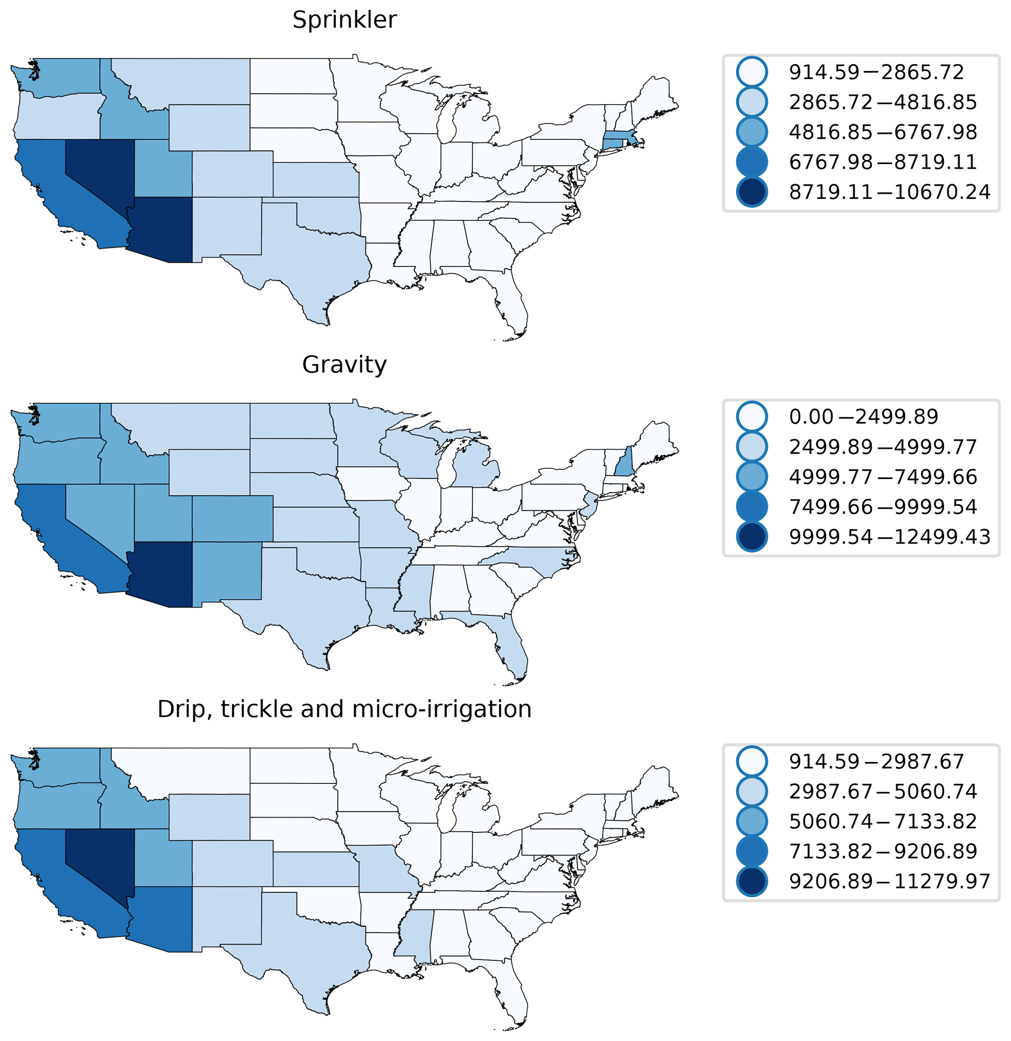
Figure A1 Per-state irrigation water application rates (m³ ha⁻¹) by irrigation technique for 2013. In accordance with Fig. 1, the data were derived from the 2013 FRIS and only reflect irrigation operations in open fields.

Figure A2 Absolute differences between the mean correlations for wet and dry periods $|r_{\mathrm{wet}}-r_{\mathrm{dry}}|$.

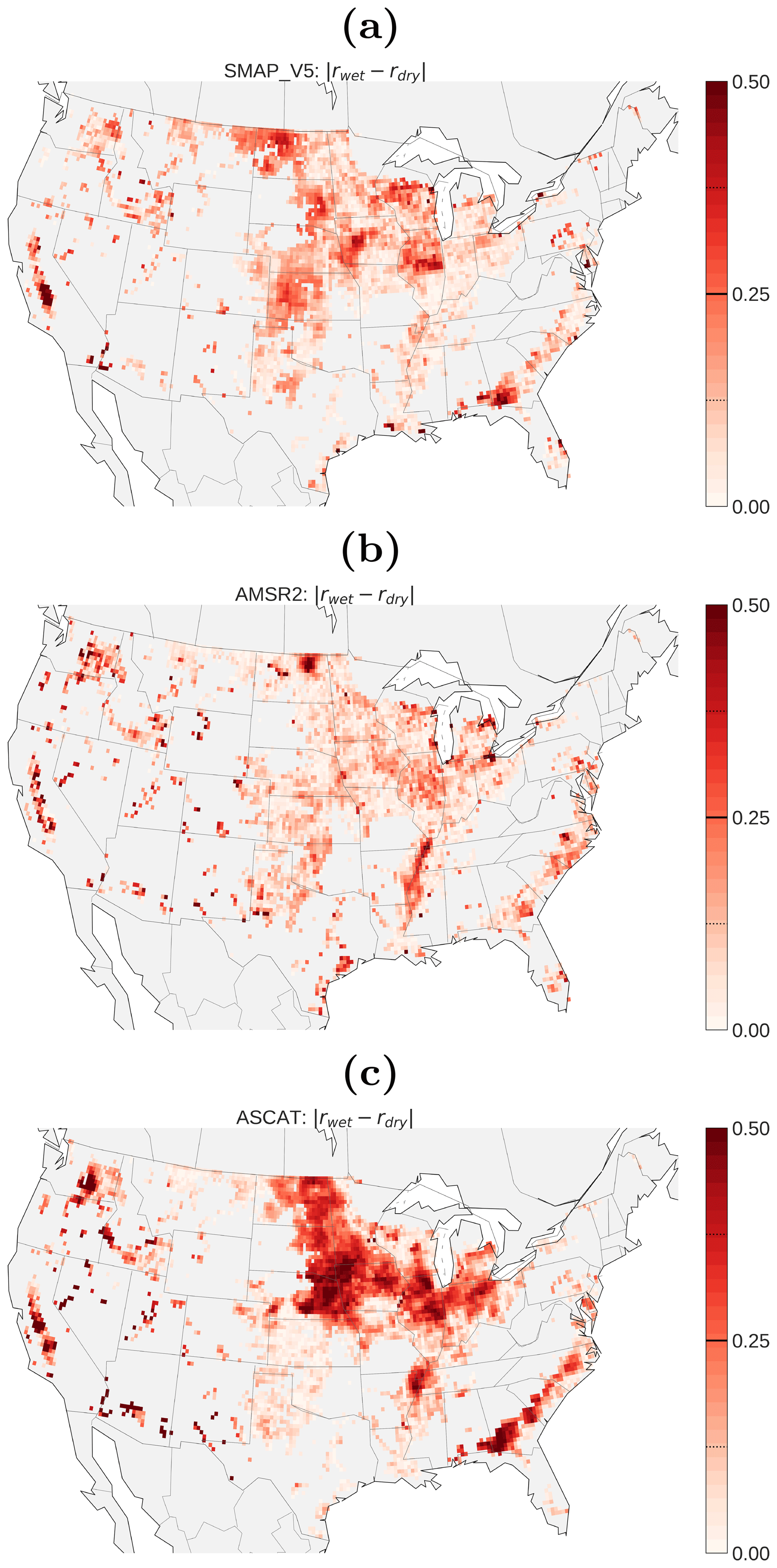
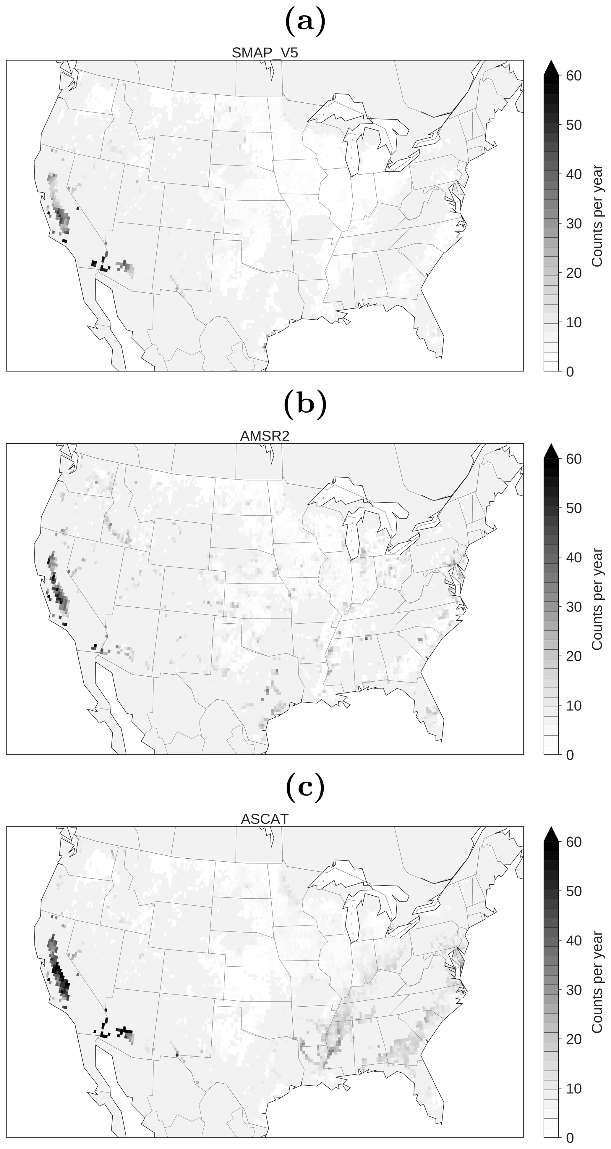
Figure A3 Mean number of days per growing season where IWU >0. Absolute counts were normalized by the number of growing seasons covered, i.e., four seasons for ASCAT and AMSR2 and two for SMAP.

Figure A4 Local optimization of the noise threshold thresh_Θ. For each focus area, the relative differences in irrigation water use ($\stackrel{\mathrm{‾}}{\mathrm{IWU}}$) estimated at a representative pixel covering a non-irrigated (PNI) and irrigated pixel (PI), respectively, $\left(\frac{{\stackrel{\mathrm{‾}}{\mathrm{IWU}}}_{\mathrm{PNI}}-{\stackrel{\mathrm{‾}}{\mathrm{IWU}}}_{\mathrm{PI}}}{{\stackrel{\mathrm{‾}}{\mathrm{IWU}}}_{\mathrm{PI}}}\right)$ are plotted against thresh_Θ choices of 0–0.2.

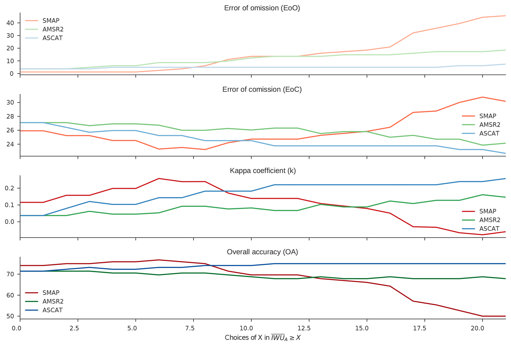
Figure A5 Determination of the binarization threshold X. Accuracy metrics were calculated between a binary representation of estimated IWU and irrigated areas based on the MIrAD-US product. Example for the State of California.