the Creative Commons Attribution 4.0 License.
the Creative Commons Attribution 4.0 License.
 | 07 Jan 2019
A large sample analysis of European rivers on seasonal river flow correlation and its physical drivers
Cristina Aguilar
Berit Arheimer
María Bermúdez
Nejc Bezak
Andrea Ficchì
Demetris Koutsoyiannis
Juraj Parajka
María José Polo
Guillaume Thirel
Alberto Montanari
The geophysical and hydrological processes governing river flow formation exhibit persistence at several timescales, which may manifest itself with the presence of positive seasonal correlation of streamflow at several different time lags. We investigate here how persistence propagates along subsequent seasons and affects low and high flows. We define the high-flow season (HFS) and the low-flow season (LFS) as the 3-month and the 1-month periods which usually exhibit the higher and lower river flows, respectively. A dataset of 224 rivers from six European countries spanning more than 50 years of daily flow data is exploited. We compute the lagged seasonal correlation between selected river flow signatures, in HFS and LFS, and the average river flow in the antecedent months. Signatures are peak and average river flow for HFS and LFS, respectively. We investigate the links between seasonal streamflow correlation and various physiographic catchment characteristics and hydro-climatic properties. We find persistence to be more intense for LFS signatures than HFS. To exploit the seasonal correlation in the frequency estimation of high and low flows, we fit a bi-variate meta-Gaussian probability distribution to the selected flow signatures and average flow in the antecedent months in order to condition the distribution of high and low flows in the HFS and LFS, respectively, upon river flow observations in the previous months. The benefit of the suggested methodology is demonstrated by updating the frequency distribution of high and low flows one season in advance in a real-world case. Our findings suggest that there is a traceable physical basis for river memory which, in turn, can be statistically assimilated into high- and low-flow frequency estimation to reduce uncertainty and improve predictions for technical purposes.
- Article
(6183 KB) - Full-text XML
-
Supplement
(142 KB) - BibTeX
- EndNote


Recent analyses for the Po River and the Danube River highlighted that catchments may exhibit significant correlation between peak river flows and average flows in the previous months (Aguilar et al., 2017). Such correlation is the result of the behaviours of the physical processes involved in the rainfall–runoff transformation that may induce memory in river flows at several different timescales. The presence of long-term persistence in streamflow has been known for a long time, since the pioneering works of Hurst (1951), and has been actively studied ever since (e.g. Koutsoyiannis, 2011; Montanari, 2012; O'Connell et al., 2016 and references therein). While a number of seasonal flow forecasting methods have been explored in the literature (e.g. Bierkens and van Beek, 2009; Dijk et al., 2013), attempts to explicitly exploit streamflow persistence in seasonal forecasting through information from past flows have been, in general, limited. Koutsoyiannis et al. (2008) proposed a stochastic approach to incorporate persistence of past flows into a prediction methodology for monthly average streamflow and found the method to outperform the historical analogue method (see also Dimitriadis et al., 2016, for theory and applications of the latter) and artificial neural network methods in the case of the Nile River. Similarly, Svensson (2016) assumed that the standardized anomaly of the most recent month will not change during future months to derive monthly flow forecasts for 1–3 months lead time and found the predictive skill to be superior to the analogue approach for 93 UK catchments. The above-mentioned persistence approach has also been used operationally in the production of seasonal streamflow forecasts in the UK since 2013, within the framework of the Hydrological Outlook UK (Prudhomme et al. 2017). A few other studies have included past flow information in prediction schemes along with teleconnections or other climatic indices (Piechota et al., 2001; Chiew et al., 2003; Wang et al., 2009). Recently, it was shown that streamflow persistence, revealed as seasonal correlation, may also be relevant for prediction of extreme events by allowing one to update the flood frequency distribution based on river flow observations in the pre-flood season and reduce its bias and variability (Aguilar et al., 2017). The above previous studies postulated that seasonal streamflow correlation may be due to the persistence of the catchments storage and/or the weather, but no attempt was made to identify the physical drivers.
The present study aims to further inspect seasonal persistence in river flows and its determinants, by referring to a large sample of catchments in six European countries (Austria, Sweden, Slovenia, France, Spain, and Italy). We focus on persistence properties of both high and low flows by investigating the following research questions: (i) what are the physical conditions, in terms of catchment properties, i.e. geology and climate, which may induce seasonal persistence in river flow, and (ii) can floods and droughts be predicted, in probabilistic terms, by exploiting the information provided by average flows in the previous months? These questions are relevant for gaining a better comprehension of catchment dynamics and planning mitigation strategies for natural hazards. To reach the above goals, we identify a set of descriptors for catchment behaviours and climate and inspect their impact on correlation magnitude and predictability of river flows.
A few studies have analysed physical drivers of streamflow persistence on annual and deseasonalized monthly and daily time series (Mudelsee, 2007; Hirpa et al., 2010; Gudmundsson et al., 2011; Zhang et al., 2012; Szolgayova et al., 2014; Markonis et al., 2018), but the topic has been less studied on intra-annual scales relevant to seasonal forecasting of floods and droughts.
To demonstrate the high practical relevance of the identified seasonal correlations we present a technical experiment for one of the studied rivers (Sect. 7) in which the frequency distribution of both high and low flows is updated one season in advance by exploiting real-time information on the state of the catchment.
The investigation of the persistence properties of river flows focuses separately on both high and low discharges and is articulated in the following steps: (a) identification of the high- and low-flow seasons, (b) correlation assessment between the peak flow in the high-flow season (average flow in the low-flow season) and average flows in the previous months, (c) analysis of the physical drivers for streamflow persistence and its predictability through a principal component analysis (PCA), and (d) real-time updating of the frequency distribution of high and low flows for a selected case study with significant seasonal correlation by employing a meta-Gaussian approach. The above steps are described in detail in the following sections.
2.1 Season identification
Season identification is performed algorithmically to identify the high-flow season (HFS) and low-flow season (LFS) for each river time series. For the estimation of HFS, we employ an automated method recently proposed by Lee et al. (2015), which identifies the high-flow season as the 3-month period centred around the month with the maximum number of occurrences of peaks over threshold (POT), with the threshold set to the highest 5 % of the daily flows. To evaluate the selection of HFS, a metric constructed as the percentage of annual maximum flows (PAMF) captured in the HFS is used. The PAMFs are classified in the subjective categories of “poor” (< 40 %), “low” (40 %–60 %), “medium” (60 %–80 %), and “high” (> 80 %) values, denoting the probability that the identified HFS is the dominant high-flow season in the record. If the identified peak month alone contains more than or equal to 80 % of the annual maxima flows, a unimodal regime is assumed and the identification procedure is terminated. In all other cases, the method allows for the search of a second peak month and the identification of a minor HFS, but we do not further elaborate on this analysis here, because we are only interested in the most extreme seasons for the purpose of predicting high and low flows.
The method proposed by Lee et al. (2015) has several advantages that make it suitable for the purpose of this research. Most importantly, it is capable of handling conditions of bimodality, which is usually a major issue for traditional methods, e.g. directional statistics (Cunderlik et al., 2004). A potential limitation is the assumption of symmetrical extension of HFS around the peak month, along with the uniform selection of its length (3-month period). The degree of subjectivity in the evaluation of the second HFS is another limitation, which is not relevant here, as we focus on the main HFS.
The LFS is herein identified as the 1-month period with the lowest amount of mean monthly flow. An alternative approach of estimating the relative frequencies of annual minima of monthly flow and selecting the month with the highest frequency as the LFS is also considered.
2.2 Correlation analysis and physical interpretation through principal component analysis
2.2.1 Correlation analysis
In the case of HFS, a correlation is sought between the maximum daily flow occurring in the HFS period and the mean flow in the previous months, before the onset of HFS. For LFS, correlation is computed between the mean flow in the LFS itself and the mean flow in the previous months. We use the mean flow in the previous month as a robust proxy of “storage” in the catchment that is expected to reflect the state of the catchment, i.e. wetter or drier than usual. Since we are interested in seasonal persistence, we compute the Pearson's correlation coefficient for HFS lag up to 9 months and for LFS lag up to 11 months.
2.2.2 Analysis of physical drivers
Catchment, geological, and climatic descriptors
An extensive investigation is carried out to identify physical drivers of seasonal streamflow correlation, in terms of catchment, geological, and climatic descriptors.
As catchment descriptors, we consider the basin area (A), the baseflow index (BI), the mean specific runoff (SR), the percentage of basin area covered by lakes (percentage of lakes – PL) and glaciers (percentage of glaciers – PG), and altitude as candidates for explanatory variables for streamflow correlation.
The area A (km2) is primarily investigated, as it is representative of the scale of the catchment, under the assumption that in larger basins the impact of the climatological and geophysical processes affecting river flow becomes more significant and may lead to a magnified seasonal correlation.
The BI is considered based on the assumption that high groundwater storage may be a potential driver of correlation. BI is calculated from the daily flow series of the rivers following the hydrograph separation procedure detailed in Gustard et al. (2008). Flow minima are sampled from non-overlapping 5-day blocks of the daily flow series, and turning points in the sequence of minima are sought and identified when the 90 % value of a certain minimum is smaller or equal to its adjacent values. Subsequently, linear interpolation is used in between the turning points to obtain the baseflow hydrograph. The BI is obtained as the ratio of the volume of water beneath the baseflow separation curve versus the total volume of water from the observed hydrograph, and an average value is computed over all the observed hydrographs for a given catchment. A low index is indicative of an impermeable catchment with rapid response, whereas a high value suggests high storage capacity and a stable flow regime.
SR (m3 s−1 km−2) is computed as the mean daily flow of the river standardized by the size of its basin area. It may be an important physical driver, as it is an indicator of the catchment's wetness. PL (%) and PG (%) are investigated for the Swedish and Austrian catchments, respectively, as lakes and glaciers are expected to increase catchment storage thus affecting persistence. Lake coverage data are based on cartography and are available from the Swedish Water Archive (https://www.smhi.se/, last access: 1 November 2016), while glacier coverage data are estimated from the CORINE land cover database (https://www.eea.europa.eu/publications/COR0-landcover, last access: 6 November 2016).
The effect of catchment altitude is also inspected using relief maps from the Shuttle Radar Topography Mission (SRTM) data (http://srtm.csi.cgiar.org/, last access: 28 July 2017). The data are available for the whole globe and are sampled at 3 arcsec resolution (approximately 90 m). Topographic information is available for all catchments located at latitudes lower than 60∘ north, while a 1 km resolution digital elevation model is available for Austria.
As geological descriptors we consider the percentage of catchment area with the presence of flysch (percentage of flysch – PF) and karstic formations (percentage of karst – PK) for Austrian and Slovenian catchments, respectively, where this type of information is available. A subset of Austrian catchments is characterized by the dominant presence of flysch, a sequence of sedimentary rocks characterized by low permeability, which is known to generate a very fast flow response. Karstic catchments, characterized by the irregular presence of sinkholes and caves, are also known for having rapid response times and complex behaviour; e.g. initiating fast preferential groundwater flow and intermittent discharge via karstic springs (Ravbar, 2013; Cervi et al., 2017). Geological features are also presumed to be linked to persistence properties, because geology is the main control for the baseflow index across the European continent (Kuentz et al., 2017). PK (%) and PF (%) are estimated from geological maps of Slovenia and Austria, respectively.
As climatic descriptors, the mean annual precipitation P (mm year−1) and the mean annual temperature T (∘C) are selected. Corresponding gridded data are retrieved from the WorldClim database (http://www.worldclim.org/, last access: 20 March 2017) at a spatial resolution of 10 arcminutes (approximately 18.55 km). We note that low mean temperature regimes are also associated with snow, the presence of which is also considered in the interpretation of the results. We also adopt the De Martonne index (IDM; De Martonne, 1926) as a climatic descriptor, which is given by and enables classification of a region into one of the following six climate classes, i.e. arid (IDM ≤5), semi-arid (5 < IDM ≤10), dry subhumid (10 < IDM ≤20), wet subhumid (20 < IDM ≤30), humid (30 < IDM ≤60), and very humid (IDM ≥60). Additionally, the Köppen–Geiger climatic classification (Kottek et al., 2006) of the rivers is assessed.
Principal component analysis
To identify which catchment, physiographic, and climatic characteristics may explain river memory, we attempt to regress the seasonal streamflow correlation on the physical descriptors introduced above. We expect the presence of multicollinearity among the predictor variables, and therefore PCA (Pearson, 1901; Hotelling, 1933) was applied to construct uncorrelated explanatory variables. In essence, PCA is an orthonormal linear transformation of p data variables into a new coordinate system of q≤p uncorrelated variables (principal components – PCs) ordered by decreasing degree of variance retained when the original p variables are projected into them (Jolliffe, 2002). Therefore, the first principal axis contains the greatest degree of variance in the data, while the second principal axis is the direction which maximizes the variance among all directions orthogonal to the first principal axis, and each succeeding component in turn has the highest variance possible while satisfying the condition of orthogonality to the preceding components. Specifically, let x be a random vector with mean μ and correlation matrix Σ, and the principal component transformation of x is then obtained as follows:
where y is the transformed vector whose kth column is the kth principal component (k=1, ), C is the p×p matrix of the coefficients or loadings for each principal component, and x′ is the standardized x vector. Standardization is applied in order to avoid the impact of the different variable units on selecting the direction of maximum variance when forming the PCs. The y values are the scores of each observation, i.e. the transformed values of each observation of the original p variables in the kth principal component direction.
PCA has useful descriptive properties of the underlying structure of the data. These properties can be efficiently visualized in the biplot (Gabriel, 1971), which is the combined plot of the scores of the data for the first two principal components along with the relative position of the p variables as vectors in the two-dimensional space. Herein, the distance biplot type (Gower and Hand, 1995), which approximates the Euclidean distances between the observations, is used. Variable vector coordinates are obtained by the coefficients of each variable for the first two principal components. After construction of the PCs, a linear regression model is explored for the case of HFS and LFS lag-1 correlation.
2.3 Technical experiment: real-time updating of the frequency distribution of high and low flows
In order to evaluate the usefulness of the information provided by the 1-month-lag seasonal correlation for flow signatures in HFS and LFS, we perform a real-time updating of the frequency distribution of high and low flows based on the average river flow in the previous month. A similar analysis for the high flows was carried out by Aguilar et al. (2017) for the Po and Danube Rivers. In principle, this is a data assimilation approach, since real-time information, i.e. observations of the average river flow, is used in order to update a probabilistic model and inform the forecast of the flow signature of the upcoming season.
In detail, a bi-variate meta-Gaussian probability distribution (Kelly and Krzysztofowicz, 1997; Montanari and Brath, 2004) is fitted between the observed flow signatures, i.e. peak flow in the HFS, QP, average flow in the LFS, QL, and the average flow in the pre-HFS and LFS months, Qm. The peak HFS flow and the average LFS flow are the dependent variables and are extracted as the peak river discharge observed in the previously identified HFS and the average river discharge observed in the previously identified LFS, respectively. The average flow in the month preceding the HFS and the LFS is the explanatory variable in both cases. In the following, random variables are denoted by an underscore and their outcomes are written in plain form.
The normal quantile transform (NQT; Kelly and Krzysztofowicz, 1997) is used in order to make the marginal probability distribution of dependent and explanatory variables Gaussian. This is achieved as follows: (a) the sample quantiles Q are sorted in increasing order, e.g. … , (b) the cumulative frequency, e.g. , is computed via a Weibull plotting position, and (c) the standard normal quantile, e.g. , is obtained as the inverse of the standard normal distribution for each cumulative frequency, e.g. G−1 (. Therefore, all sample quantiles are discretely mapped into the Gaussian domain. To get the inverse transformation for any normal quantile, we connect the points in the above mapping with linear segments. The extreme segments are extended to allow extrapolation outside the range covered by the observed sample.
In the Gaussian domain, a bi-variate Gaussian distribution is fitted between the random explanatory variable NQm and the dependent variables NQP and NQL by assuming the stationarity and ergodicity of the variables. We define the generic random variable NQfs to represent any dependent flow signature, i.e.; NQP and NQL in our case. Then, the predicted signature at time t can be written as
where ρ(NQm, NQfs) is the Pearson's cross-correlation coefficient between NQm and NQfs, h is the selected correlation lag with h=1 in the present application, and Nε(t) is an outcome of the stochastic process Nε, which is independent, homoscedastic, stochastically independent of NQm, and normally distributed with zero mean and variance 1−ρ2(NQm, NQfs). Then, the joint bi-variate Gaussian probability distribution function is defined by the mean (μ(NQm) =0 and μ(NQfs)=0), the standard deviation (σ(NQm)=1 and σ(NQfs)=1) of the standardized normalized series, and the Pearson's cross-correlation coefficient between the normalized series, ρ(NQm, NQfs). From the Gaussian bi-variate probability properties, it follows that for any observed NQm(t−h) the probability distribution function of NQfs(t) conditioned on NQm is Gaussian, with parameters given by
To derive the probability distribution of Qfs(t) conditioned to the observed Qm(t−h), we first apply the inverse NQT, i.e. we use linear segments to connect the points of the previous discrete quantile mapping of the original quantiles into the Gaussian domain, and accordingly, obtain Qfs(t) for any NQfs(t). Subsequently, we estimate the parameters of an assigned probability distribution for the obtained quantiles in the untransformed domain. This is referred to as the updated probability distribution of the considered flow signature (NQP and NQL, in our case). We use the extreme value type I distribution for the peak flows and calculate the differences in the magnitude of estimated maxima for a given return period between the unconditioned and the updated distribution. The latter is conditioned by the 95 % sample quantile of the observed mean flow in the previous month. To model the low flows we use the log-normal distribution, which was found to exhibit the best fit for the river in question among other typical candidates for average flows, i.e. the Weibull and Gamma distribution. The low flows are conditioned by the lower 5 % sample quantile of the observed mean flow in the previous month.
Table 1Summary statistics of the river descriptors. Summary statistics for PL, PG, and PF variables are computed only for the subset of catchments with positive values (the total number of catchments is also reported in brackets next to the values). PK is used as a categorical variable (PK is either higher or lower than 50 % of catchment area), therefore sample statistics are not computed in this case, but the number of stations with PK ≥ 50 % is reported as “positive” presence of karst.
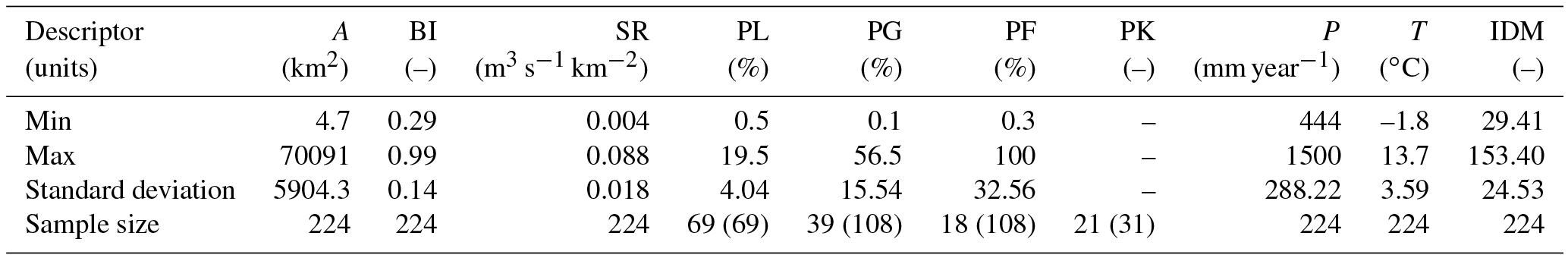

Figure 1Updated Köppen–Geiger climatic map for period 1951–2000 (Kottek et al., 2006) showing the location of the 224 river gauge stations.
The dataset includes 224 records spanning more than 50 years of daily river flow observations from gauging stations, mostly from non-regulated streams. A few catchments are impacted by regulation. Among the 224 rivers, 108 are located in Austria, 69 in Sweden, 31 in Slovenia, 13 in France, two in Spain, and one in Italy. Catchment areas vary significantly, the largest being the Po River basin in Italy (70 091 km2) and the smallest being the Hallabäcken River basin in Sweden (4.7 km2). The geographical location of the river gauge stations as well as their climatic classification are shown in Fig. 1. Most of the examined rivers belong to either a warm temperate (C) or a boreal or snow climate (D) with a subset impacted by polar climatic conditions (E), according to the updated world map of the Köppen–Geiger climate classification (Fig. 1) based on gridded temperature and precipitation data for the period 1951–2000 (Kottek et al., 2006). More specifically, the majority of French and Slovenian and approximately one third of the Swedish basins belong to the warm temperate Cfb category characterized by precipitation distributed throughout the year (fully humid) and warm summers. The rest of the Swedish catchments are impacted by a Dfc climatic type, i.e. a snow climate, fully humid with cool summers. The Austrian catchments belonging to the region impacted by the European Alps have the most complicated regime due to their topographic variability. At the lowest altitudes, Cfb is the prevailing regime, but as proximity to the Alps increases, a Dfc regime dominates, and progressively, in the highest altitude basins, the climate becomes a polar tundra type (Et), characterized primarily by the very low temperatures present. The characteristics of all the climatic regimes of the studied rivers are given in the legend of Fig. 1. A summary of the river basins under study, in terms of the selected descriptors, is also provided in Table 1, showing that the investigated rivers cover a wide range of catchment area sizes, flow regimes, and climatic conditions.
It is relevant to note that 16 of the Austrian rivers are subject to regulation, which may alter the persistence properties of river flows. This relates to generally “mild” forms of regulation, i.e. upstream regulation with a very low degree of flow attenuation, hydropower operations, and flow diversions to and from the basin. A preliminary examination of these rivers did not reveal any significant change during time of the flow regime. The presence of regulation does not preclude the exploitation of correlation for predicting river flows in probabilistic terms, but it may affect the analysis of physical drivers, as it may enhance or reduce persistence in the natural river flow regime. Given that detailed information is generally lacking on the impact of regulation (Kuentz et al. 2017), we assume stationarity of the river flows for all the catchments herein considered and, additionally, assume that river management does not significantly affect the identification of the physical drivers.
4.1 Season identification
Approximately half of the 224 rivers are characterized by at least one high-flow season with medium or higher significance (PAMF of HFS ≥ 60 %). Among them, very strong unimodal regimes (PAMF of HFS ≥ 80 %) are observed in 63 rivers, the majority of which are located in Sweden. For 25 % of the rivers, a high-flow season of low significance is found (PAMF of HFS between 40 %–60 %), while for the remaining 25 % the high-flow distribution looks uniform throughout the year. Bimodality regimes are found with low and moderate significance in rivers located mostly in Austria and Sweden, but we focus here on the major high-flow season, as we are interested in the most extreme events. A minor HFS analysis would be perhaps relevant in other regions of the world where bimodal flood regimes are more prominent, as suggested by the analysis of Lee et al. (2015).
Regarding the LFS identification, the two considered approaches (see Sect. 2.1) agree for 139 out of 224 stations, but the first method, i.e. the 1-month period with the lowest amount of mean monthly flow, is selected as being more relevant to the purpose of computing mean flow correlations.
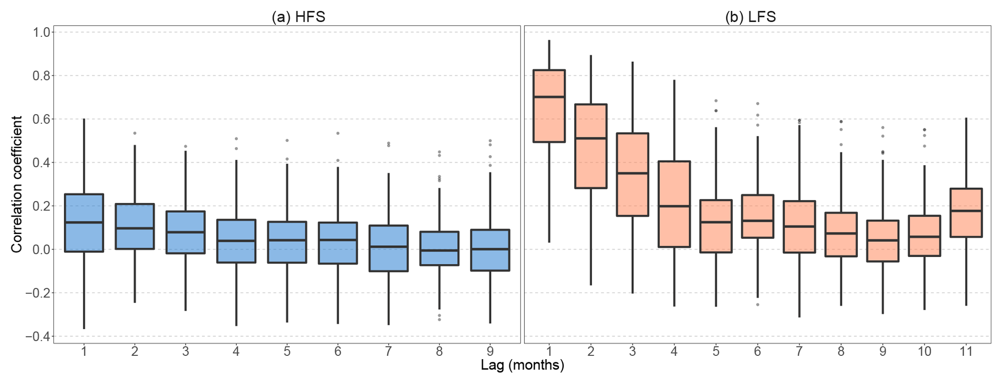
Figure 2Box plots of seasonal correlation coefficient against lag time for HFS (a) and LFS (b) analysis for the 224 rivers. The lower and upper ends of the box represent the first and third quartiles, respectively, and the whiskers extend to the most extreme value within 1.5 IQR (interquartile range) from the box ends; outliers are plotted as filled circles.
4.2 Seasonal correlation
LFS correlation is markedly higher than the corresponding HFS correlation for lags 1–6, and its median remains higher than 0 for more lags (see Fig. 2). For the case of HFS correlation, we focus only on the most significant first lag, for which 73 rivers are found to have correlation significantly higher than 0 at a 5 % significance level. In Fig. 3, the autocorrelation of the whole monthly series is compared to the LFS correlation for lag of 1 and 2 months, in order to prove that the seasonal correlation for LFS is significantly higher than its counterpart computed by considering the whole year. The latter is also confirmed by the Kolmogorov–Smirnov test for both LFS lags (corresponding p values, and for the null hypothesis that the LFS correlation coefficients are not higher than the corresponding values for the monthly series autocorrelation; Conover, 1971).
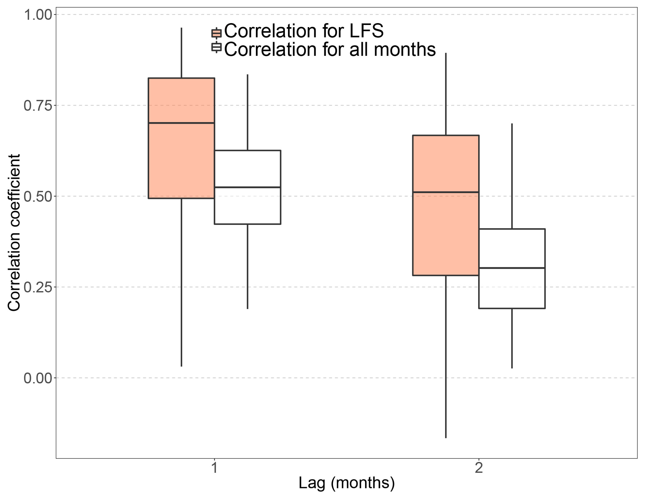
Figure 3Box plots of lag-1 and lag-2 correlation coefficients for LFS analysis (orange) and the whole monthly series (white) for the 224 rivers. The lower and upper ends of the box represent the first and third quartiles, respectively, and the whiskers extend to the most extreme value within 1.5 IQR (interquartile range) from the box ends.
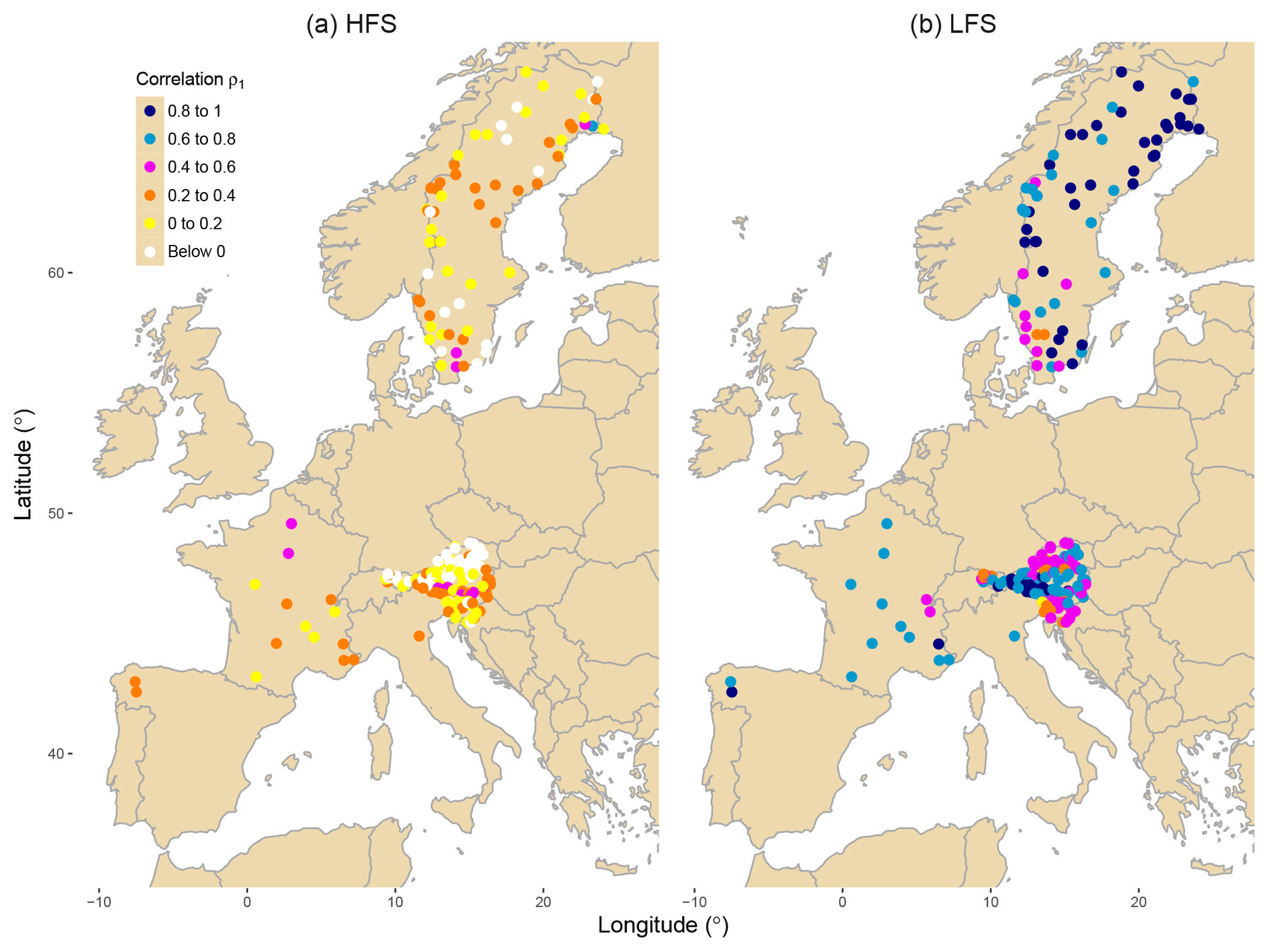
Figure 4Spatial distribution of the lag-1 correlation coefficients for HFS (a) and LFS (b) analysis. Legend shows the colour assigned to each class of correlation for the data.
Figure 4 shows the spatial pattern of HFS and LFS streamflow correlations. It is interesting to notice the emergence of spatial clustering in the correlation magnitude, which implies its dependence on different spatially varying physical mechanisms. For example, for HFS, a geographical pattern emerges within France, since the highest correlation coefficients are located in the northern part of the country, which is characterized by an oceanic climate and higher baseflow indices.
To attribute the detected correlations to physical drivers, we define six groups of potential drivers of seasonal correlation magnitude: basin size, flow indices, the presence of lakes and glaciers, catchment elevation, catchment geology, and hydro-climatic forcing. For some of the descriptors the information is only available for a few countries.
In what follows, we will use the term “positive (negative) impact on correlation” to imply that an increasing value of the considered descriptor is associated with increasing (decreasing) correlation. For each descriptor, we also report, between parentheses, the Spearman's rank correlation coefficient rs (Spearman, 1904) between its value and the considered (LFS or HFS) correlation and the p value of the null hypothesis rs=0. Spearman's coefficient is adopted in view of its robustness to the presence of outliers and its capability of capturing monotonic relationships of the non-linear type.
5.1 Catchment area – descriptor A
Figure 5 shows that there is only a weak positive impact of the catchment area (log transformed) on correlation for HFS (rs=0.17, p=0.01) but a more significant positive one for LFS (rs=0.27, ). The presence of relevant scatter in the plots also indicates that it is not a key determinant of correlation.
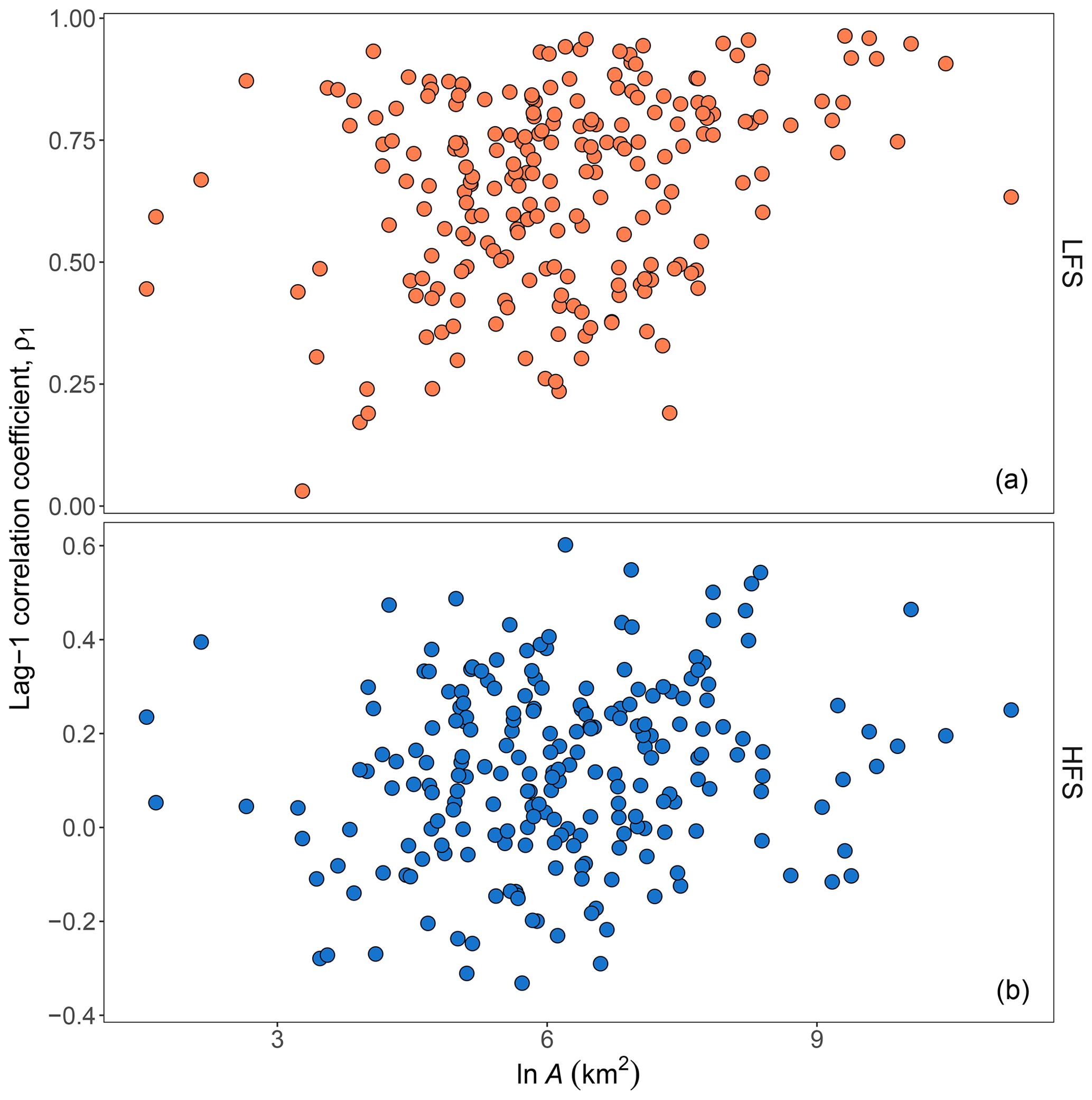
Figure 5Scatter plots of lag-1 HFS (b) and LFS (a) streamflow correlation versus the natural logarithm of basin area ln A.
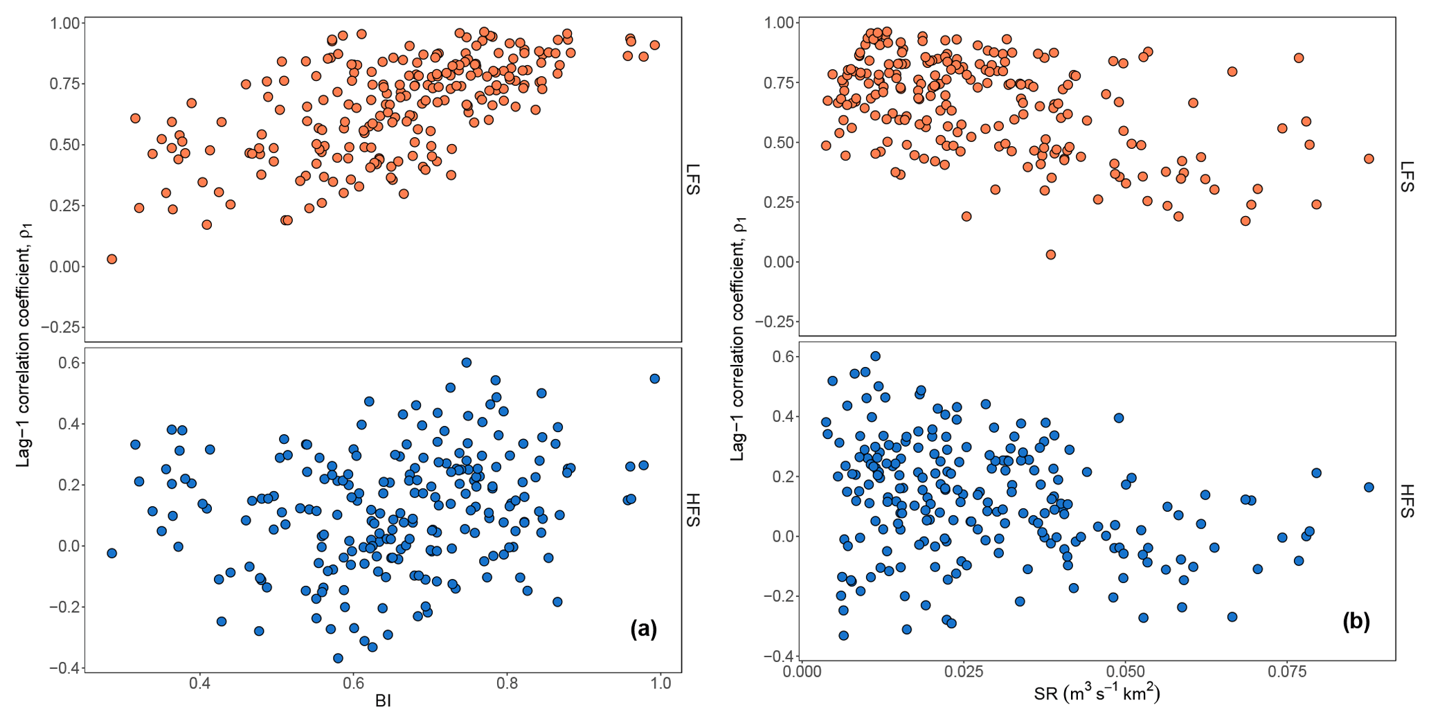
Figure 6Scatter plots of lag-1 HFS (bottom panels) and LFS streamflow correlation (a) versus baseflow index (BI) (a) and specific runoff (SR) (b).
5.2 Flow indices – descriptors BI and SR
The effect of the BI and SR is shown in Fig. 6. The BI (Fig. 6a) appears to be a marked positive driver for LFS (rs=0.6, ), while its effect for HFS is less clear, being weakly positive (rs=0.21, p=0.001). For SR (Fig. 6b), it appears that both LFS and HFS streamflow correlations drop for increasing wetness (, and respectively).
5.3 Presence of lakes and glaciers – descriptors PL and PG
Detailed information on the presence of lakes is available for the 69 Swedish catchments, while the areal extension of glaciers is known for the 108 Austrian catchments. Figure S1 in the Supplement shows that the impact of lake area (Fig. S1a) on correlation for LFS and HFS is not significant but positive (, and ). The results for glaciers show a positive impact for LFS () but a negative impact for HFS (). For a meaningful interpretation, these results should be considered in conjunction with the seasonality of flows for the Austrian catchments. Low flows for the glacier-dominated catchments typically occur in winter months, when glaciers are not contributing to the flow (Parajka et al., 2009). Thus the observed result for LFS more likely portrays the impact of low temperature (low evapotranspiration) and snow accumulation, the latter generally being a slowly varying process. For HFS, which typically occurs in the summer months for the considered catchments, flows are mainly determined by snowmelt, which is associated to reduced persistence (Fig. S1b).
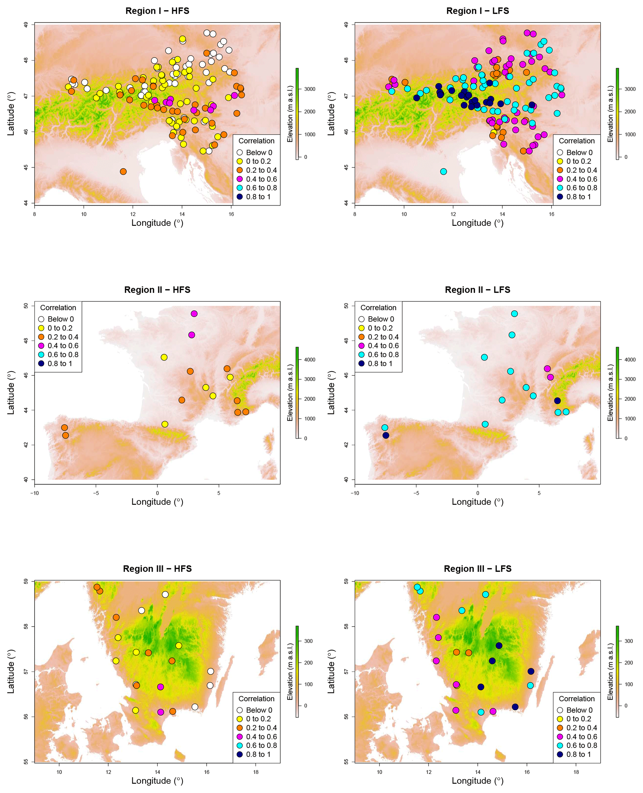
Figure 7Relief maps from SRTM elevation data for the HFS and LFS lag-1 correlations of the rivers. Note that elevation scale is different for each region. Legend shows the colour assigned to each class of correlation for the data.

Figure 8Digital elevation model of the Austrian river network depicting the spatial distribution of lag-1 positive correlation for HFS (a) and lag-1 positive correlation for LFS (b). Legend shows the colour assigned to each class of correlation for the data.
5.4 Catchment elevation
The areal coverage of the SRTM data is limited to 60∘ N and 54∘ S, therefore data for the northern part of the Swedish catchments are not available. The rest of the rivers are divided in three regions based on proximity: Region I, including the central and eastern part of the Alps and encompassing Austrian, Slovenian, and Italian catchments; Region II, including the western part of the Alps and encompassing French and Spanish territory; and Region III, including the southern part of Sweden. Figure 8 shows elevation maps along with the location of gauge stations and magnitude of correlations. Elevation seems to enhance LFS correlation, which is more evident in the mountainous Region I (Fig. 7). For HFS correlation there is not a prevailing pattern.
In the case of Austrian catchments, a 1 km resolution digital model is also used to extract information on elevation. Figure 8 confirms that there is a positive correlation pattern emerging with elevation for LFS. Based on local climatological information, it can be concluded that the spatial pattern for LFS correlation is reflective of the timing and strength of seasonality of the low flows in Austria, where dry months occur in lowlands during the summer due to increased evapotranspiration and in the mountains during winter (mostly February) due to snow accumulation which is characterized by stronger seasonality compared to the lowlands flow regime (Parajka et al., 2016; see Fig. 1). Concerning HFS in the same region, high flows are significantly impacted by the seasonality of extreme precipitation (Parajka et al., 2010), which is highly variable, with the exception of the rivers where high flows are generated by snowmelt. Therefore, a spatially consistent pattern does not clearly emerge.

Figure 9Box plots of lag-1 correlation for Slovenian rivers with more than 50 % presence of karstic formations (PK) and rivers with no or less presence for HFS analysis (a) and LFS analysis (b). The lower and upper ends of the box represent the first and third quartiles, respectively, and the whiskers extend to the most extreme value within 1.5 IQR (interquartile range) from the box ends.
5.5 Catchment geology – descriptors PK and PF
Two different geological behaviours are identified which may impact river correlation. We first focus on 21 Slovenian catchments (out of 31) where more than 50 % of the basin area is characterised by the presence of karstic aquifers (percentage of karstic areas PK ≥ 50 %). Figure 9 shows box plots of the estimated lag-1 correlation coefficient for both HFS and LFS against rivers where PK < 50 %. It is clear that there is a significant decrease in correlation where karstic areas dominate for both for HFS and LFS.
In a second analysis, we focus on Austrian catchments and investigate the relationship between correlation and percentage of flysch coverage, PF. Figure S2 shows that there is not a prevailing pattern in either case ( for LFS, and for HFS).
5.6 Atmospheric forcing – descriptors P and T
Figure 10 shows the lag-1 HFS and LFS correlations against estimates of the annual precipitation P and annual mean temperature T as well as the IDM. LFS correlation appears to be more sensitive than HFS to the above climatic indices, showing a decrease with increasing temperature and also a decrease with increasing precipitation ( for P, and for T). HFS correlation is scarcely sensitive to these variables ( for P, and for T). The IDM (Fig. 10c) shows a mild decrease of both LFS () and HFS correlation with increasing IDM (), while for the latter there seems to be a clearer trend (lower correlation with higher IDM) in very humid areas (dark blue points in Fig. 10c).
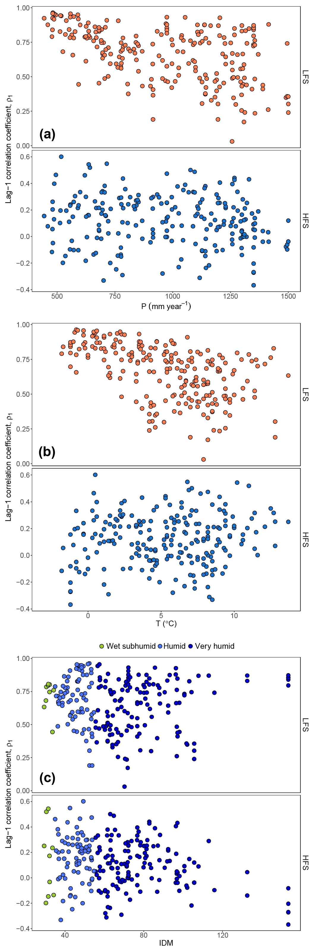
Figure 10Scatter plots of lag-1 HFS and LFS correlation versus annual precipitation P (a), mean annual temperature T (b), and De Martonne index (IDM) (c).
Table 2Differences in the mean values between the descriptors of the group 20-highest-correlation-river group for HFS and LFS versus the remaining rivers (204). NL, NG, NF, and NK columns contain the absolute number of rivers in the higher correlation group with the specific descriptor (presence of lake, glacier, flysch, and karst ), with ∗ denoting significance at 5 % significance level (two-sided test), and brackets in the body of the table containing the mean value from the 1000 resampled 20-catchment subsets.
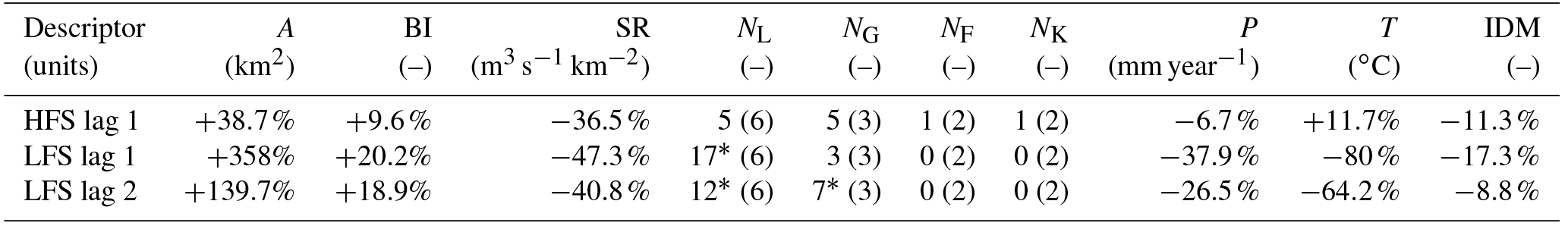
5.7 Physical drivers of high correlation
To gain further insight into the results we select the 20 catchments with the highest streamflow seasonal correlation coefficients for both HFS and LFS periods in order to investigate their physical characteristics in relation to the remaining set of rivers. Table 2 summarizes statistics for selected descriptors in order to identify dominant behaviours. We also compare the number of rivers with distinctive features, i.e. lakes NL (number of rivers with lakes), glaciers NG (number of river with glaciers), flysch NF (number of rivers with flysch formations) and karst NK (number of rivers with karstic areas), for the highest correlation group with those obtained from 1000 randomly sampled 20-catchment groups from the whole set of considered catchments to assess whether higher correlation implies distinctive features.
By focusing on HFS, one can notice that the catchments with higher seasonal correlation are characterized by larger catchment area; higher baseflow index and temperature with respect to the remaining catchments; and lower specific runoff, precipitation, and wetness. The presence of lake, glacier, karstic, and flysch areas do not appear significantly effective at a 5 % significance level. More robust considerations can be drawn for the LFS; higher seasonal correlation is found for larger catchments with a higher baseflow index and lower specific runoff, precipitation, and wetness. Decreasing temperature is strongly associated with higher correlation for the LFS. The presence of lakes plays a significant role, both for lag-1 and lag-2 correlations, with the latter also being significantly influenced by the presence of glaciers.
Table 3Loadings of the three principal components for ln A, SR, BI, and T. The explained variance of each PC is denoted in parenthesis.
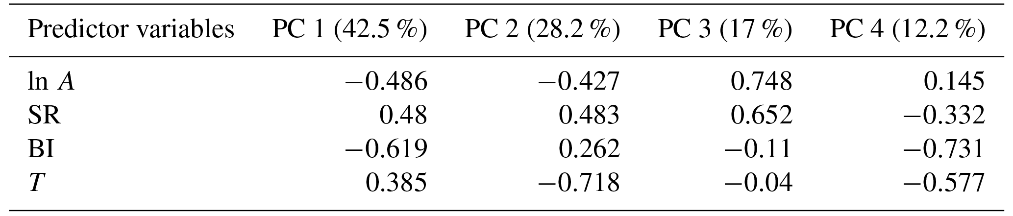
We attempt to fit a linear regression model to relate correlation to physical drivers, in order to support correlation estimation for ungauged catchments. To avoid the impact of multicollinearity in the regression while additionally summarizing river information, we apply PCA (see Sect. 2.2). Although correlation effects are efficiently dealt with via the PCA, we avoid including highly correlated variables in the analysis. For example, the De Martonne index, precipitation and SR are mutually highly correlated (all Pearson's cross-correlations are higher than 0.6), therefore we only consider the SR in the PCA because it shows a more robust linear relationship with correlation magnitude. We select A, BI, SR, and T as the variables to be considered in the PCA. A log transformation is applied to the basin area to reduce the impact of outliers. Table 3 shows the coefficients estimated for each component (the loadings) and the explained variance. The first principal component is primarily a measure of BI, the second principal component mostly accounts for T, and the third principal component accounts for A. There is an evident geographical pattern emerging by the visualization of countries in the biplot (Fig. 11). Slovenian rivers cluster towards the direction of increasing SR and T, whereas Swedish rivers cluster towards the opposite direction of increasing BI and decreasing T. Austrian rivers, which are the majority, are the most diverse. The first two components together explain 70 % of the total variability in the data.
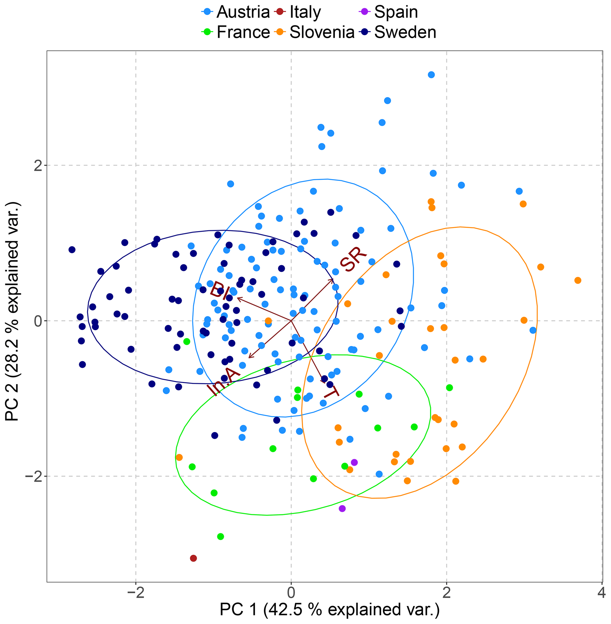
Figure 11Principal component distance biplot showing the principal component scores on the first two principal axes along with the vectors (brown arrows) representing the coefficients of the baseflow index (BI), specific runoff (SR), natural logarithm of basin area ln A, and mean annual temperature T variables when projected on the principal axes. Scores for the rivers are plotted in different colours corresponding to each country of origin, and 68 % normal probability contour plots are plotted for the countries.
Naturally, the statistical behaviour of the indices reflects the known local controls for certain rivers. For example, the observed lowest BI in Slovenia is consistent with the presence of karstic formations for the majority of the Slovenian rivers, as is the higher BI in Sweden and Austria, which is related to the presence of lakes and glaciers in both countries.
Table 4Summary of linear regression results for the LFS model. ∗ indicates a 0.1 % significance level.

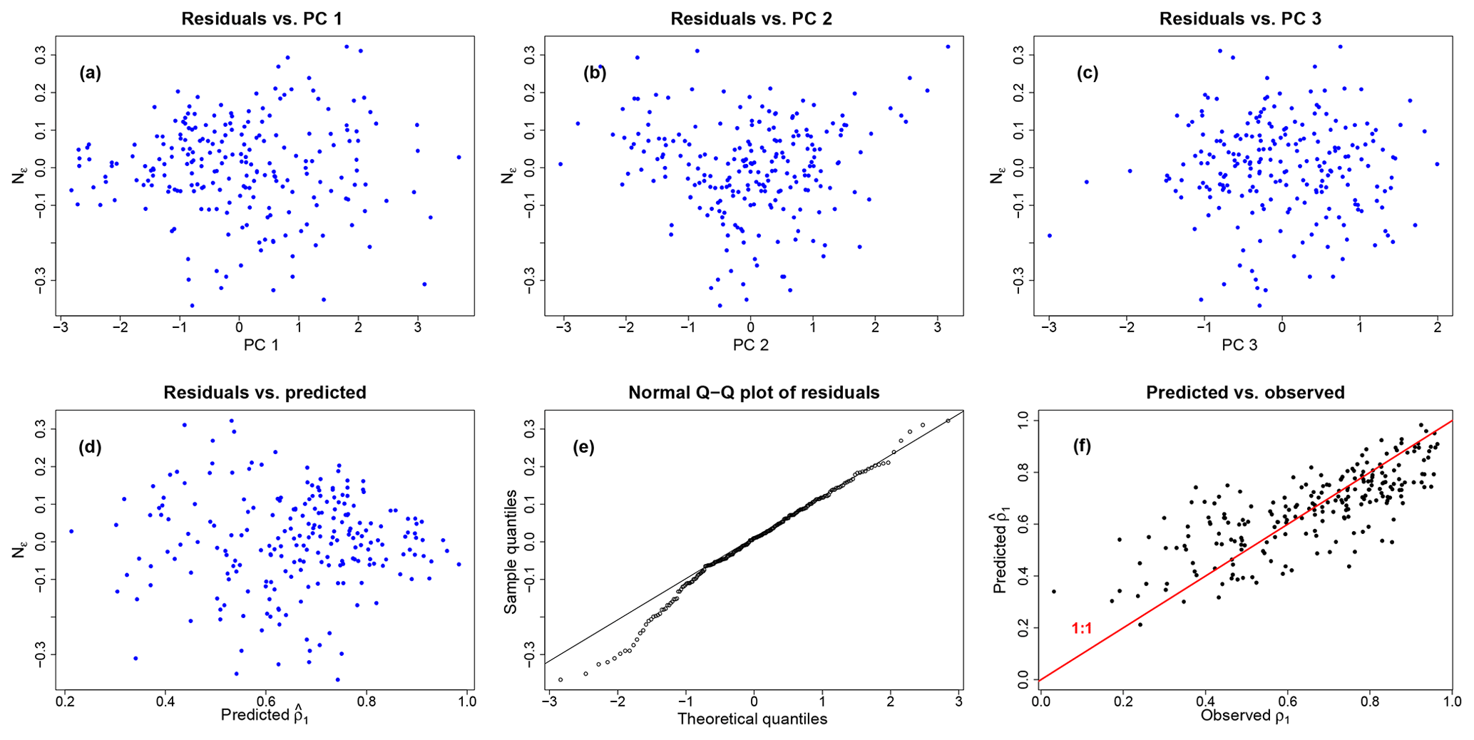
Figure 12Diagnostic plots of linear regression for the LFS model. Residuals versus the first (a), the second (b), and the third principal component (c) as well as the predicted values (d). Normal Q–Q plot of the residuals (e). Plot of the predicted values from linear regression versus the observed ones; red line is the diagonal line 1 : 1 (f).
In the case of HFS, all the examined linear models (combinations of ln A, SR, BI, P, T, and IDM predictors) failed in explaining the streamflow correlation magnitude. On the contrary, the linear regression model performs fairly well in explaining the correlation for LFS, with an adjusted R2 value of 0.58 and an F test returning a p value < . The coefficients for the first three PCs are found significantly different from zero at a 0.1 % significance level and are included in the regression (see Table 4). The highest coefficient is obtained for the first PC, which mostly accounts for BI importance. Diagnostic plots from linear regression for LFS are shown in Fig. 12. There is no clear violation of the homoscedasticity assumption in linear regression, apart from the presence of a limited number of outliers. There is a certain departure from normality in the lower tail of the residuals, which relates to the fact that the model performs better in the area of higher seasonal streamflow correlations and overestimates the lower correlations.
We apply the technical experiment (see Sect. 2.3) for high and low flows to the Oise River in France and assess the difference in the estimated flood and low-flow magnitudes. We update the probability distribution of high and low flows after the occurrence of the upper 95 % and lower 5 % sample quantile of the observed mean flow in the previous month, respectively.
The Oise River (55 years of daily flow values) at Sempigny in France has a basin area of 4320 km2, and its gauging station at Sempigny is part of the French national real-time monitoring system (https://www.vigicrues.gouv.fr/, last access: 23 July 2018), which is in place to monitor and forecast floods in the main French rivers. The selected river has a high technical relevance, since it experiences both types of extremes with large impacts. For instance, a severe drought event in 2005 led to water restrictions impacting agriculture and water uses in the region (Willsher, 2005), while the river originated an inundation during the 1993 flood events in northern and central France, which was one of the most catastrophic flood-related disasters in Europe in the period 1950–2005 (Barredo, 2007). It is characterized by HFS correlation ρ=0.54, which is the third largest lag-1 correlation for the HFS in our dataset, and LFS correlation ρ=0.80, which stands for the 70 % quantile of the sample lag-1 correlation for LFS.
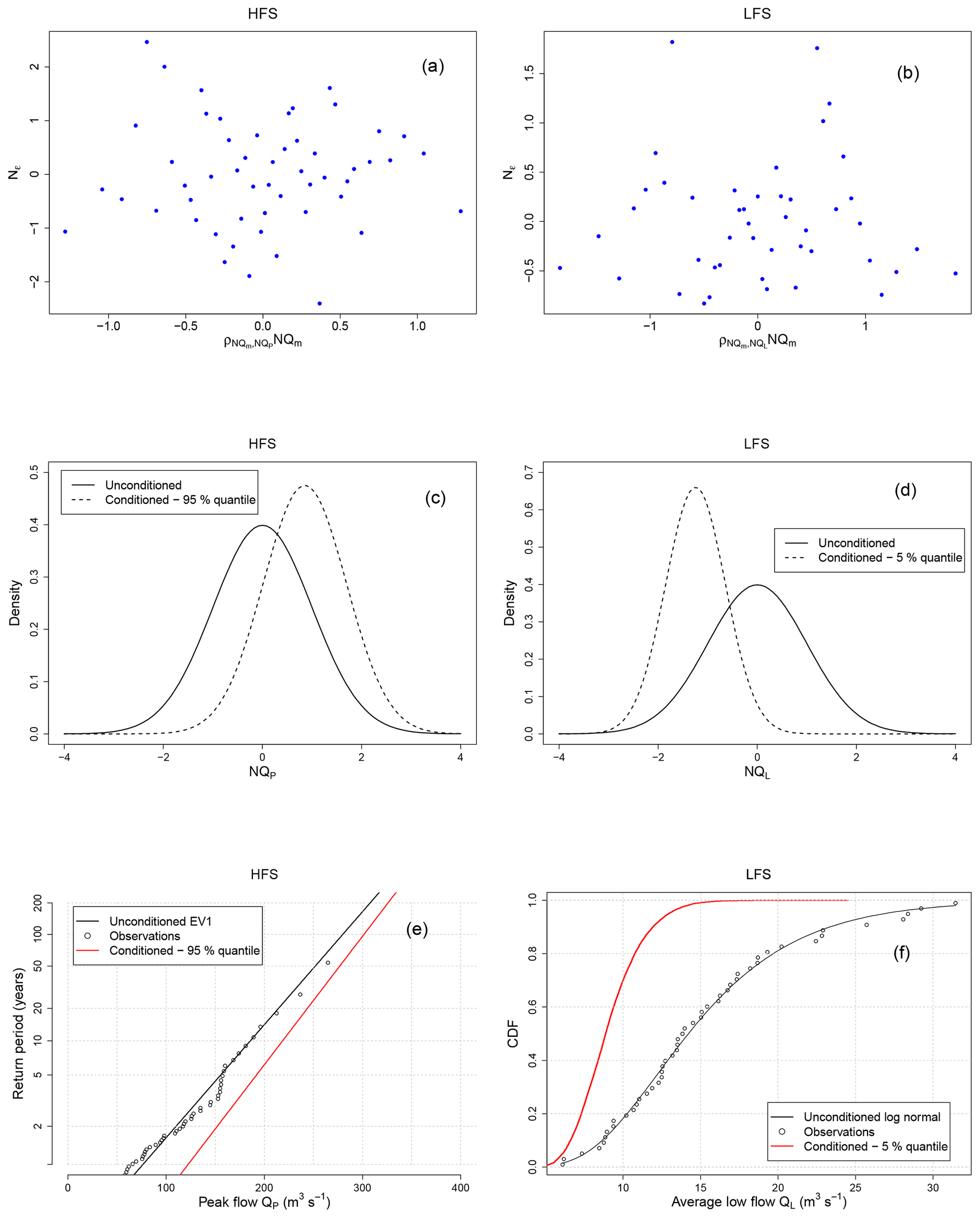
Figure 13Conditioning the frequency distributions for high and low flows for the Oise River. Plots of the residuals of the linear regression given by Eq. (2) for the HFS (a) and LFS (b) models. Probability distribution of the unconditioned normalized peak flows NQP (solid line) and the normalized peak flows NQP conditioned to the occurrence of the 95 % quantile (dotted line) for the HFS (c), and probability distribution of the unconditioned normalized low flows NQL (solid line) and the normalized low flows NQL conditioned to the occurrence of the 5 % quantile (dotted line) for the LFS (d). Gumbel probability plots of the return period versus the unconditioned peak flows QP (black line), and the peak flows QP modelled by the EV1 distribution and conditioned to the occurrence of the 95 % quantile (red line) for the HFS (e). Cumulative distribution function of the unconditioned low flows QL (black line) and the low flows QL modelled by the log-normal distribution and conditioned to the occurrence of the 5 % quantile (red line) for the LFS (f).
A visual inspection of the residual plots is also performed (Fig. 13a, b) in order to evaluate the assumption of homoscedasticity of the residuals of the regression models given by Eq. (2). The residuals do not show any apparent trend, and the Gaussian linear model is therefore accepted. Figure 13c, d shows the conditioned and unconditioned probability distributions of peak and low flows in the Gaussian domain. As follows from Eqs. (3) and (4), the variance of the updated (conditioned) distributions decreases while the mean value increases.
After application of the inverse NQT the conditioned peak flows are modelled through the EV1 distribution and compared to the unconditioned (observed) peak flows. The corresponding Gumbel probability plot for conditioned and unconditioned distributions is shown in Fig. 13e. For the return period of 200 years, the updated distribution shows a 6 % increase in the flood magnitude for the Oise River (307.7 to 326.44 m3 s−1). Likewise, the conditioned low flows are modelled through the log-normal distribution. The two cumulative distribution functions are compared in Fig. 13f, showing a major departure in the estimated quantiles for the updated distribution; the occurrence of the predefined 5 % quantile flow in the pre-LFS month induces a decrease of the exceedance probability of an average LFS flow of 15 m3 s−1 from a prior 43 % (according to the unconditioned model) to 1 %.
The methodology presented herein aims to progress our physical understanding of seasonal river flow persistence for the sake of exploiting the related information to improve probabilistic prediction of high and low flows. The correlation of average flow in the previous months with the LFS flow and HFS peak flow was found to be relevant, with the former prevailing over the latter. This result was foreseen, since the LFS correlation refers to average flow, while the HFS correlation is related to rapidly occurring events. We also aim to investigate physical drivers for correlation and quantify their relative impact on correlation magnitude. Therefore, a thorough investigation of the geophysical and climatological features of the considered catchments was carried out.
We found that the increasing basin area and baseflow index are associated with increasing seasonal streamflow correlation, yet the latter has a stronger impact. To this respect, Mudelsee (2007), Hirpa et al. (2010), and Szolgayova et al. (2014) also found positive dependencies of long-term persistence on basin area, and Markonis et al. (2018) found a positive impact too, but for larger spatial scales (> 2×10⁴ km2), while Gudmunsson et al. (2011) found basin area to have negligible to no impact on the low-frequency components of runoff. Our results additionally point out that catchment storage induces mild positive correlation, not only for low discharges which are directly governed by base flow, but also for high flows, which is less anticipated.
Previous studies also pointed out that correlation increases for groundwater-dominated regimes (Yossef et al., 2013; Dijk et al., 2013; Svensson, 2016) and slower catchment response times (Bierkens and van Beek, 2009), which concurs with the impact of the baseflow index found herein as well as with the observed impact of fast responding karst areas. The latter findings are also in agreement with our conclusion that correlation decreases with increasing rapidity of river flow formation, which, for instance, occurs in the presence of karstic areas and wet soils, explaining why persistence decreases with high specific runoff, as also confirmed by other studies (Gudmundsson et al., 2011; Szolgayova et al., 2014).
Other contributions also reported higher streamflow persistence in drier conditions, either relating to lower specific runoff or mean areal precipitation estimates (Szolgayova et al., 2014; Markonis et al., 2018). It was postulated that this is due to wet catchments showing increased short-term variability compared to drier catchments (Szolgayova et al., 2014) and having a faster response to rainfall due to saturated soil. A similar conclusion has been reached by other previous studies reporting that low humidity catchments are more sensitive to interannual rainfall variability (Harman et al., 2011), therefore leading to enhanced persistence. Yet, these studies refer to generally humid regions and cannot be extrapolated to more arid climates. A related conclusion is proposed by Seneviratne et al. (2006), who found the highest soil moisture memory for intermediate soil wetness. These results do not contrast with our findings, which refer to a wide range of climatic conditions. In fact, our finding that increased wetness has a negative impact on seasonal memory of both high and low flows extends the above results to the seasonal scale and, interestingly, to both types of extremes.
We also confirm the role of lakes in determining higher catchment storage and therefore positive correlations for the LFS, which has only been reported for annual persistence in a few sites (Zhang et al., 2012).
The effect of snow cover for lag-1 LFS correlation is also revealed by the Austrian catchments. The mountainous rivers, directly affected by the process of snow accumulation, exhibit winter LFS and higher correlation than the rivers in the lowlands, which are more prone to drying out due to evapotranspiration in the hotter summer months. The inspection of elevation data confirmed the role of high altitudes in increasing LFS correlation, which is likely related to storage effects due to snow accumulation and gradual melting. In this respect, Kuentz et al. (2017) found that topography exerts dominant controls over the flow regime in the larger European region, controlling the flashiness of flow and being a particularly important driver for other low-flow signatures too. In fact, topography may affect the flow regime directly, through flow routing, but also indirectly, because of orographic effects in precipitation and hydro-climatic processes affected by elevation (e.g. snowmelt and evapotranspiration).
Regarding atmospheric forcing, we find LFS correlation to be negatively correlated to mean areal temperature and annual precipitation. The former result may be explained, considering that increased evapotranspiration (higher temperature) is likely to dry out LFS flows while snow coverage (lower temperature) was found to be associated with higher LFS correlation. An apparently different conclusion was drawn by Szolgayova et al. (2014a) and Gudmundsson et al. (2011), who reported increasing persistence with increasing mean temperature postulating that snow-dominated flow regimes smooth out interannual fluctuations. Yet, it should be noted that they refer to interannual variability, while we refer here to seasonal correlation and therefore to shorter timescales, which imply a different dynamic of snow accumulation and snowmelt; latitude may also play a relevant role in this, since in southern Europe the complete ablation of snow can occur more than once during the cold season, and sublimation may account for 20 %–30 % of the annual snowfall (Herrero and Polo, 2016), decreasing the amount of snowmelt and impacting LFS flows in the summer season.
Snowmelt mechanisms are found to increase predictive skill during low-flow periods in some other studies (Bierkens and van Beek, 2009; Mahanama et al., 2011; Dijk et al., 2013). However, in the glacier-dominated regime of western Alpine and central Austrian catchments, it is unlikely that this is a relevant driver of higher correlation, since low flow occurs in the winter months. Yet the mountainous, glacier-dominated rivers still show increased LFS correlation compared to rivers in the lowlands, which agrees well with other studies that have found less uncertainty in the rainfall–runoff modelling in this regime owing to the greater seasonality of the runoff process and the decreased impact of rainfall compared to the rainfall-dominated regime of the lowlands (e.g. Parajka et al., 2016).
Although the considerable uncertainty of areal precipitation estimates should be acknowledged, the contribution of annual precipitation interestingly complements the negative effect of increasing specific runoff –which is highly correlated to P estimates– on the correlation magnitude for both LFS and HFS. This outcome confirms that catchments receiving significant amount of rainfall do show less correlation than drier regimes as discussed before.
This research investigates the presence of persistence in river flow at the seasonal scale, the associated physical drivers, and the prospect for employing the related information to improve probabilistic prediction of high and low flows by exploring a large sample of European rivers. The main findings are summarized below:
-
Rivers in Europe show persistent features at the seasonal timescale, manifested as correlation between high- and low-flow signatures, i.e. peak flows in HFS, average flows in LFS, and average flows in the previous month. Correlation for LFS signatures is found to be consistently higher than HFS.
-
Seasonal correlation shows increased spatial variability together with spatial clustering.
-
Storage mechanisms, groundwater-dominated basins, and slower catchment response time, as reflected by large basin areas, a high baseflow index, and the presence of lakes, amplify seasonal correlation. On the contrary, correlation is lower in quickly responding karstic basins and increased wetness conditions, as revealed by high specific runoff.
-
Low mean areal temperature is associated with higher LFS correlation owing to the weaker drying-out evapotranspiration force and the mechanism of snow accumulation in higher altitudes. Higher mean areal precipitation is associated with lower LFS predictability, possibly due to the presence of saturated conditions and increased short-term variability in wetter climates.
-
The drivers of LFS predictability are easier to identify and allow for the opportunity to construct regression models for possible application to ungauged basins (see Sect. 6).
-
HFS and LFS correlation may directly apply to the probabilistic prediction of “extremes”, i.e. high and low flows, as increased correlation can be exploited in various stochastic models. Such an application was performed in Sect. 7 in a data assimilation setting for a river of marked technical relevance.
Regarding the last point, once a significant correlation is identified, it may be exploited in other model variants as well, e.g. adding more dependent variables of lagged flow and/or coupling with other relevant explanatory variables, such as teleconnections or antecedent rainfall, in multivariate prediction schemes. Indeed, the presence of river memory at the seasonal scale represents a possible opportunity to improve the prediction of water-related natural hazards by reducing uncertainty of associated estimates and allowing significant lag time for decision-making and hazard prevention. Besides the high relevance for extremes, this type of seasonal predictability could also be of interest to the management of water resources by, for instance, exploring the memory properties of a minor HFS.
The inspection of the physical basis, apart from advancing our understanding of the catchment dynamics and enabling predictions in ungauged basins, is highly important, as it may guide the search for other dependent variables and build confidence in the formation of process-based stochastic models (Montanari and Koutsoyiannis, 2012). A large sample of indices was herein inspected, yet more data are necessary in order to allow for more certain and generalized conclusions worldwide. An important note is the effect of regulation, which, due to the lack of objective data, is not completely understood. However, the opportunity of exploiting correlation is not affected by the presence of regulation, provided that the management of river flow does not change in time.
We conclude that our results point out that river memory provides interesting information that holds both theoretical and operational potential to improve the understanding and prediction of extremes, support decision-making, and increase the level of preparedness for water-related natural hazards.
The data and code used in this study may be made available to the readers upon request to the corresponding author.
The supplement related to this article is available online at: https://doi.org/10.5194/hess-23-73-2019-supplement.
The authors declare that they have no conflict of interest.
The present work was (partially) developed within the framework of the Panta
Rhei Research Initiative of the International Association of Hydrological
Sciences (IAHS). Part of the results were elaborated in the Switch-On Virtual
Water Science Laboratory that was developed in the context of the SWITCH-ON
(Sharing Water-related Information to Tackle Changes in the Hydrosphere –
for Operational Needs) project, funded by the European Union Seventh
Framework Programme (FP7/2007-2013) under grant agreement no. 603587. Nejc Bezak
gratefully acknowledges funding by the Slovenian Research Agency
(grants J2-7322 and P2-0180). María Bermúdez gratefully acknowledges
financial support from the Spanish Regional Government of Galicia,
Postdoctoral Grant Program 2014.
Edited by:
Louise Slater
Reviewed by: three anonymous referees
Aguilar, C., Montanari, A., and Polo, M.-J.: Real-time updating of the flood frequency distribution through data assimilation, Hydrol. Earth Syst. Sci., 21, 3687–3700, https://doi.org/10.5194/hess-21-3687-2017, 2017.
Barredo, J. I.: Major flood disasters in Europe: 1950–2005, Nat. Hazards, 42, 125–148, https://doi.org/10.1007/s11069-006-9065-2, 2007.
Bierkens, M. F. P. and van Beek, L. P. H.: Seasonal Predictability of European Discharge: NAO and Hydrological Response Time, J. Hydrometeorol., 10, 953–968, https://doi.org/10.1175/2009JHM1034.1, 2009.
Cervi, F., Blöschl, G., Corsini, A., Borgatti, L., and Montanari, A.: Perennial springs provide information to predict low flows in mountain basins, Hydrolog. Sci. J., 62, 2469–2481, https://doi.org/10.1080/02626667.2017.1393541, 2017.
Chiew, F. H. S., Zhou, S. L., and McMahon, T. A.: Use of seasonal streamflow forecasts in water resources management, J. Hydrol., 270, 135–144, https://doi.org/10.1016/S0022-1694(02)00292-5, 2003.
Conover, W. J.: Practical Nonparametric Statistics, New York, John Fliley and Sons. Inc, 1971.
Cunderlik, J. M., Ouarda, T. B., and Bobée, B.: Determination of flood seasonality from hydrological records/Détermination de la saisonnalité des crues à partir de séries hydrologiques, Hydrolog. Sci. J., 49, 511–526, https://doi.org/10.1623/hysj.49.3.511.54351, 2004.
De Martonne, E. M.: L'indice d'aridité, Bulletin de l'Association de géographes français, 3, 3–5, https://doi.org/10.3406/bagf.1926.6321, 1926.
Dijk, A. I., Peña-Arancibia, J. L., Wood, E. F., Sheffield, J., and Beck, H. E.: Global analysis of seasonal streamflow predictability using an ensemble prediction system and observations from 6192 small catchments worldwide, Water Resour. Res., 49, 2729–2746, https://doi.org/10.1002/wrcr.20251, 2013.
Dimitriadis, P., Koutsoyiannis, D., and Tzouka, K.: Predictability in dice motion: how does it differ from hydro-meteorological processes?, Hydrolog. Sci. J., 61, 1611–1622, https://doi.org/10.1080/02626667.2015.1034128, 2016.
Gabriel, K. R.: The biplot graphic display of matrices with application to principal component analysis, Biometrika, 58, 453–467, https://doi.org/10.1093/biomet/58.3.453, 1971.
Gower, J. C. and Hand, D. J.: Biplots, CRC Press, London, UK, 1995.
Gudmundsson, L., Tallaksen, L. M., Stahl, K., and Fleig, A. K.: Low-frequency variability of European runoff, Hydrol. Earth Syst. Sci., 15, 2853–2869, https://doi.org/10.5194/hess-15-2853-2011, 2011.
Gustard, A. and Demuth, S.: Manual on low-flow estimation and prediction, World Meteorological Organization, Geneva, Switzerland, 2008.
Harman, C. J., Troch, P. A., and Sivapalan, M.: Functional model of water balance variability at the catchment scale: 2. Elasticity of fast and slow runoff components to precipitation change in the continental United States, Water Resour. Res., 47, 2, https://doi.org/10.1029/2010WR009656, 2011.
Herrero, J. and Polo, M. J.: Evaposublimation from the snow in the Mediterranean mountains of Sierra Nevada (Spain), The Cryosphere, 10, 2981–2998, https://doi.org/10.5194/tc-10-2981-2016, 2016.
Hirpa, F. A., Gebremichael, M., and Over, T. M.: River flow fluctuation analysis: Effect of watershed area, Water Resour. Res., 46, 12, https://doi.org/10.1029/2009WR009000, 2010.
Hotelling, H.: Analysis of a complex of statistical variables into principal components, J. Educ. Psychol., 24, 417–441, https://doi.org/10.1037/h0071325, 1933.
Hurst, H. E.: Long-term storage capacity of reservoirs, Trans. Amer. Soc. Civil Eng., 116, 770–808, 1951.
Jolliffe, I.: Principal component analysis, Wiley Online Library, New York, USA, https://doi.org/10.1002/9781118445112.stat06472, 2002.
Kelly, K. S. and Krzysztofowicz, R.: A bivariate meta-Gaussian density for use in hydrology, Stoch. Hydrol. Hydraul., 11, 17–31, https://doi.org/10.1007/BF02428423, 1997.
Kottek, M., Grieser, J., Beck, C., Rudolf, B., and Rubel, F.: World Map of the Köppen-Geiger climate classification updated, Meteorol. Z., 15, 259–263, https://doi.org/10.1127/0941-2948/2006/0130, 2006.
Koutsoyiannis, D.: Hurst-Kolmogorov Dynamics and Uncertainty, J. Am. Water Resour. As., 47, 481–495, https://doi.org/10.1111/j.1752-1688.2011.00543.x, 2011.
Koutsoyiannis, D., Yao, H., and Georgakakos, A.: Medium-range flow prediction for the Nile: a comparison of stochastic and deterministic methods/Prévision du débit du Nil à moyen terme: une comparaison de méthodes stochastiques et déterministes, Hydrolog. Sci. J., 53, 142–164, https://doi.org/10.1623/hysj.53.1.142, 2008.
Kuentz, A., Arheimer, B., Hundecha, Y., and Wagener, T.: Understanding hydrologic variability across Europe through catchment classification, Hydrol. Earth Syst. Sci., 21, 2863–2879, https://doi.org/10.5194/hess-21-2863-2017, 2017.
Lee, D., Ward, P., and Block, P.: Defining high-flow seasons using temporal streamflow patterns from a global model, Hydrol. Earth Syst. Sci., 19, 4689–4705, https://doi.org/10.5194/hess-19-4689-2015, 2015.
Mahanama, S., Livneh, B., Koster, R., Lettenmaier, D., and Reichle, R.: Soil Moisture, Snow, and Seasonal Streamflow Forecasts in the United States, J. Hydrometeor., 13, 189–203, https://doi.org/10.1175/JHM-D-11-046.1, 2011.
Markonis, Y., Moustakis, Y., Nasika, C., Sychova, P., Dimitriadis, P., Hanel, M., Máca, P., and Papalexiou, S. M.: Global estimation of long-term persistence in annual river runoff, Adv. Water Resour., 113, 1–12, https://doi.org/10.1016/j.advwatres.2018.01.003, 2018.
Montanari, A.: Hydrology of the Po River: looking for changing patterns in river discharge, Hydrol. Earth Syst. Sci., 16, 3739–3747, https://doi.org/10.5194/hess-16-3739-2012, 2012.
Montanari, A. and Brath, A.: A stochastic approach for assessing the uncertainty of rainfall-runoff simulations, Water Resour. Res., 40, 1, https://doi.org/10.1029/2003WR002540, 2004.
Montanari, A. and Koutsoyiannis, D.: A blueprint for process-based modeling of uncertain hydrological systems, Water Resour. Res., 48, 9, https://doi.org/10.1029/2011WR011412, 2012.
Mudelsee, M.: Long memory of rivers from spatial aggregation, Water Resour. Res., 43, 1, https://doi.org/10.1029/2006WR005721, 2007.
O'Connell, P. E., Koutsoyiannis, D., Lins, H. F., Markonis, Y., Montanari, A., and Cohn, T.: The scientific legacy of Harold Edwin Hurst (1880–1978), Hydrolog. Sci. J., 61, 1571–1590, https://doi.org/10.1080/02626667.2015.1125998, 2016.
Parajka, J., Kohnová, S., Merz, R., Szolgay, J., Hlavčová, K., and Blöschl, G.: Comparative analysis of the seasonality of hydrological characteristics in Slovakia and Austria/Analyse comparative de la saisonnalité de caractéristiques hydrologiques en Slovaquie et en Autriche, Hydrolog. Sci. J., 54, 456–473, https://doi.org/10.1623/hysj.54.3.456, 2009.
Parajka, J., Kohnová, S., Bálint, G., Barbuc, M., Borga, M., Claps, P., Cheval, S., Dumitrescu, A., Gaume, E., Hlavčová, K., and Merz, R.: Seasonal characteristics of flood regimes across the Alpine–Carpathian range, J. Hydrol., 394, 78–89, https://doi.org/10.1016/j.jhydrol.2010.05.015, 2010.
Parajka, J., Blaschke, A. P., Blöschl, G., Haslinger, K., Hepp, G., Laaha, G., Schöner, W., Trautvetter, H., Viglione, A., and Zessner, M.: Uncertainty contributions to low-flow projections in Austria, Hydrol. Earth Syst. Sci., 20, 2085–2101, https://doi.org/10.5194/hess-20-2085-2016, 2016.
Pearson, K.: On lines and planes of closest fit to systems of points in space, Phil. Mag., 2, 559–572, https://doi.org/10.1080/1478644010946272, 1901.
Piechota, T. C., Chiew, F. H., Dracup, J. A., and McMahon, T. A.: Development of exceedance probability streamflow forecast, J. Hydrol. Eng., 6, 20–28, https://doi.org/10.1061/(ASCE)1084-0699(2001)6:1(20), 2001.
Prudhomme, C., Hannaford, J., Harrigan, S., Boorman, D., Knight, J., Bell, V., Jackson, C., Svensson, C., Parry, S., and Bachiller-Jareno, N.: Hydrological Outlook UK: an operational streamflow and groundwater level forecasting system at monthly to seasonal time scales, Hydrolog. Sci. J., 62, 2753–2768, https://doi.org/10.1080/02626667.2017.1395032, 2017.
Ravbar, N.: Variability of groundwater flow and transport processes in karst under different hydrologic conditions/Spremenljivost Pretakanja Voda in Prenosa Snovi V Krasu ob Razlicnih Hidroloskih Pogojih, Acta Carsologica, 42, 327, https://doi.org/10.3986/ac.v42i2.644, 2013.
Seneviratne, S. I., Koster, R. D., Guo, Z., Dirmeyer, P. A., Kowalczyk, E., Lawrence, D., Liu, P., Mocko, D., Lu, C.-H., Oleson, K. W., and Verseghy, D.: Soil moisture memory in AGCM simulations: analysis of global land–atmosphere coupling experiment (GLACE) data, J. Hydrometeorol., 7, 1090–1112, https://doi.org/10.1175/JHM533.1, 2006.
Spearman, C.: The Proof and Measurement of Association between Two Things, Am. J. Psychol., 15, 72–101, https://doi.org/10.2307/1412159, 1904.
Svensson, C.: Seasonal river flow forecasts for the United Kingdom using persistence and historical analogues, Hydrolog. Sci. J., 61, 19–35, https://doi.org/10.1080/02626667.2014.992788, 2016.
Szolgayova, E., Laaha, G., Blöschl, G., and Bucher, C.: Factors influencing long range dependence in streamflow of European rivers, Hydrol. Process., 28, 1573–1586, https://doi.org/10.1002/hyp.9694, 2014.
Wang, Q. J., Robertson, D. E., and Chiew, F. H. S.: A Bayesian joint probability modeling approach for seasonal forecasting of streamflows at multiple sites, Water Resour. Res., 45, 5, https://doi.org/10.1029/2008WR007355, 2009.
Willsher, K.: France brings in water rationing after worst drought for 30 years, The Guardian, available at: https://www.theguardian.com/environment/2005/jul/11/weather.france (last access: 30 July 2018), 2005.
Yossef, N. C., Winsemius, H., Weerts, A., Beek, R., and Bierkens, M. F.: Skill of a global seasonal streamflow forecasting system, relative roles of initial conditions and meteorological forcing, Water Resour. Res., 49, 4687–4699, https://doi.org/10.1002/wrcr.20350, 2013.
Zhang, Q., Zhou, Y., Singh, V. P., and Chen, X.: The influence of dam and lakes on the Yangtze River streamflow: long-range correlation and complexity analyses, Hydrol. Process., 26, 436–444, https://doi.org/10.1002/hyp.8148, 2012.
- Abstract
- Introduction
- Methodology
- Data and catchment description
- River memory analysis for the considered case studies
- Physical interpretation of correlation
- Principal component analysis of the predictors and linear regression
- Real-time updating of the frequency distribution of high and low flows for the Oise River
- Discussion
- Conclusions and outlook
- Code and data availability
- Competing interests
- Acknowledgements
- References
- Supplement