Evaluation of drought representation and propagation in regional climate model simulations across Spain

Drought is an important climatic risk that is expected to increase in frequency, duration, and severity as a result of a warmer climate. It is complex to model due to the interactions between atmospheric and continental processes. A better understanding of these processes and how the current modelling tools represent them and characterize drought is vital.

The aim of this study is to analyse how regional climate models (RCMs) represent meteorological, soil moisture, and hydrological drought as well as propagation from precipitation anomalies to soil moisture and streamflow anomalies. The analysis was carried out by means of standardized indices calculated using variables directly related to each type of drought: precipitation (SPI), soil moisture (SSMI), runoff (SRI), and streamflow (SSI).

The RCMs evaluated are the CNRM-RCSM4, COSMO-CLM, and PROMES. All of the simulations were obtained from the Med-CORDEX database and were forced with ERA-Interim. The following datasets were used as references: SAFRAN (meteorological drought), offline land surface model simulations from ISBA-3L and ORCHIDEE (soil moisture drought), a SIMPA hydrological model simulation, and observed streamflow (hydrological drought).

The results show that RCMs improve meteorological drought representation. However, uncertainties are identified in their characterization of soil moisture and hydrological drought, as well as in drought propagation. These are mainly explained by the model structure. For instance, model structure affects the temporal scale at which precipitation variability propagates to soil moisture and streamflow.

1 Introduction

Impacts from recent climate-related extremes show that ecosystems and human systems are significantly vulnerable and exposed to current climate variability (IPCC, 2014). In addition, most of these impacts have been observed to increase in climate change scenarios. For instance, drought frequency has increased in Mediterranean regions during recent decades (Mariotti, 2010; Sousa et al., 2011; Hoerling et al., 2012).

Drought is a complex phenomenon with important impacts on the environment (Reichstein et al., 2013; Vicente-Serrano et al., 2013) as well as on society and the economy (FAO, 2009; Owens et al., 2003). The latter case, corresponds to socioeconomic drought and is outside the scope of this paper. There are several types of drought (IPCC, 2007; Mishra and Singh, 2010; Van Loon, 2015) depending on which part of the system suffers from water deficit:

• meteorological drought, which corresponds to a period during which precipitation is considerably lower than its average level;

• soil moisture drought (also known as agricultural drought), which is due to a deficit of water in the soil's unsaturated zone, making it impossible to cover the crop's needs;

• and hydrological drought, which occurs when runoff, streamflow, and water levels in rivers, lakes, and groundwater are low. A more precise definition refers to superficial and groundwater water availability decreases in managed systems, affecting water demand.

As precipitation deficits propagate through the hydrological system (Wilhite, 2000; Van Loon et al., 2012b), drought types are interrelated. Soil moisture drought is slightly out of phase with meteorological drought in non-irrigated areas and depends on several factors, such as the soil type and capacity to retain water as well as actual evapotranspiration. This is also applicable to regions where irrigation is carried out under unusual circumstances, for example, to avoid crop loss. In irrigated areas, soil moisture drought is directly related to the availability of irrigation water and therefore depends on hydrological drought. Hydrological drought is also affected by meteorological drought but generally at a larger temporal scale than soil moisture drought. Therefore, each system component is characterized by its own propagation dynamics and memory.

A better understanding of the different types of drought and their propagation processes is key to improving current and future drought representation and, thus, drought prediction and management tools. Regional climate models (RCMs) can help in this task. One of their greatest advantages is their adaptation to the regional scale (Feser et al., 2011). This allows us to use regional observations and to increase the model's physical parametrization complexity. Such models are suitable for drought analyses performed at the scale of large river basins. Another important aspect of RCMs is that these models are used to develop regional climate change scenarios via downscaling processes (Jiménez-Guerrero et al., 2013). In addition, using high resolution permits RCMs to be used to perform studies of atmospheric phenomena at a small scale. However, drought is difficult to model, as complex interactions between atmospheric and continental surface processes must be combined with human action (Van Loon et al., 2012a). Furthermore, the relationships among drought types add complexity to such modelling.

Drought studies have gained interest in recent years due to increasing concern regarding (i) complexity in hydrological resource management, (ii) the escalation of the frequency, severity, and duration of extreme events, (iii) the increase in both the vulnerability to such events and the probability of being affected by them, and (iv) climate change (Andreadis and Lettenmaier, 2006; Mishra and Singh, 2010, 2011; López-Bustins et al., 2013; Jenkins and Warren, 2014). Drought studies are normally performed using drought indices, among which the Palmer drought severity index (PDSI) (Palmer, 1965) and the standardized precipitation index (SPI) (McKee et al., 1993) are two of the most widely used. According to Farahmand and AghaKouchak (2015), standardized indices can be computed using other variables besides precipitation. For instance, Xu et al. (2018) used data from the Soil Moisture Active Passive (SMAP) satellite and the North American Land Data Assimilation System (NLDAS) to compute a standardized soil moisture index for drought warning. Shukla and Wood et al. (2008) calculated a standardized runoff index using a simulation from the Variable Infiltration Capacity (VIC) model. They compared its behaviour to that of the SPI and concluded that a runoff-based index has the potential to complement other climate indices. Vicente-Serrano et al. (2012) analysed a method to compute a standardized streamflow index to compare streamflow hydrological conditions both spatially and temporally in a precise way.

Several studies analyse meteorological drought by means of RCMs. For instance, Maule et al. (2013) used the SPI and a version of the PDSI to analyse drought representation by 14 RCMs from the ENSEMBLES project (van der Linden and Mitchell, 2009) at a European scale. Blenkinshop and Fowler (2007a, b) analysed drought characteristics using RCMs from the PRUDENCE project (Christensen et al., 2007) across Britain and at a European scale by means of the drought severity index (DSI). PaiMazumder et al. (2013) and Masud et al. (2017) analysed projected changes to drought aspects in Canadian prairies by means of RCMs. The first study used three severity drought indices, whereas the second one used the SPI and PDSI. Other studies employed RCMs to analyse drought trends (Wu et al., 2016) or to study the capacity of downscaled data to represent drought spells (Anagnostopoulou, 2017). RCMs are also used in soil moisture and hydrological drought analyses. However, there have been fewer studies about these types of drought. Vu et al. (2015) and Meresa et al. (2016) studied hydrometeorological drought by computing precipitation and runoff standardized indices using simulations of the Weather Research and Forecasting (WRF) RCM driven by general climate models (GCMs). Wang et al. (2011) studied the impact of climate change on drought. They analysed drought characteristics and propagation impacts on meteorological, soil moisture, and hydrological droughts in Illinois using GCM-RCM nested simulations. Soil moisture and hydrological drought are also analysed by setting a given accumulated period to compute the drought index. García-Valdecasas Ojeda et al. (2017) studied how the WRF model improved dry and wet period detection using the SPI and the standardized precipitation–evapotranspiration index (SPEI) computed at 3- and 12-month timescales to study episodes related to soil moisture and hydrological droughts. Vicente-Serrano (2006) used the SPI to analyse drought spatial patterns as a function of the timescales used in the index computation. For this, the SPI was computed at several timescales to detect soil moisture and hydrological droughts. Other studies that analysed the effect of the accumulated period are Vicente-Serrano and López-Moreno (2005) and Edossa et al. (2009).

Taking into account the different types of drought analyses performed with RCMs and the need to better understand droughts at the current time, but also in the future, the regional modelling tools must be evaluated. The work presented here has two objectives:

• to analyse how RCMs characterize meteorological, soil moisture, and hydrological drought;

• and to analyse how RCMs represent the propagation from a precipitation anomaly to a soil moisture and streamflow anomaly.

While the first objective aims towards contributing to drought representation analysis by RCMs, the second one assesses how these models simulate drought propagation. The latter objective is a key issue for the understanding of drought that has not been fully analysed from a RCM perspective. In this study, each type of drought is characterized using standardized indices that define drought according to the variability in a given variable: precipitation (meteorological drought), soil moisture (soil moisture drought), and streamflow and total runoff (hydrological drought). The work carried out analyses three RCMs: (i) the “Centre National de Recherche Météorologique” regional climate system model (CNRM-RCSM4, Sevault et al., 2014; Nabat et al., 2014), (ii) the COnsortium for Small-scale MOdelling (COSMO) model in CLimate Mode (COSMO-CLM, Rockel et al., 2008), and (iii) PROMES (Castro et al., 1993; Sánchez et al., 2004; Domínguez et al., 2010). The reference data used are (i) the “Système d'Analyse Fournissant des Renseignements Atmosphériques à la Neige” (SAFRAN) atmospheric analysis (Quintana-Seguí, 2015), (ii) LSM offline simulations from the three-layer version of the “Interaction Sol-Biosphère-Atmosphère” (ISBA-3L) (Quintana-Seguí et al., 2019) and the Organising Carbon and Hydrology In Dynamic EcosystEms (ORCHIDEE) models, (iii) a simulation from the “Sistema Integrado de Modelización Precipitación-Aportación” (SIMPA) hydrological model (Estrela and Quintas, 1996; Ruiz, 1999), and (iv) observed streamflow.

2 Area and study period

This study was carried out across mainland Spain, which is known to experience frequent droughts (Olcina, 2001). The time period was limited to the availability of RCM simulations and observations: from 1989 to 2008 for the meteorological and soil moisture drought and from 1989 to 2005 for the hydrological drought.

Precipitation across mainland Spain is complex (Serrano et al., 1999) and highly influenced by relief. The main climatic regimes are oceanic and Mediterranean. However, a semiarid climate or even a desert-like climate can be identified in the southeast (Aemet, 2011). In general, Spain is a semiarid region and is not densely vegetated. As a result, soil moisture displays a large annual cycle. From a hydrological point of view, there is a strong dependence of the main rivers on the precipitation generated in the nearby relief and the resulting runoff. An example is in the Ebro Basin and the Pyrenees. In addition, the impact of the anthropic effect must be taken into account because there is a wide network of dams and river canals that, in some cases, operate between basins.

According to Sousa et al. (2011), drought in Spain has increased in severity and frequency. Although precipitation does not show significant annual trends, observations show a reduction in spring and summer (de Luis et al., 2010) as well as an increase in the number of consecutive dry days (Turco and Llasat, 2011). Both aspects have an impact on soil moisture drought, which is also affected by an increase in annual and seasonal temperatures (del Rio et al., 2011; Kenawy et al., 2013). This rise in temperature increases the atmospheric demand (Vicente-Serrano et al., 2014) and thus evapotranspiration, reducing the soil's water content. For hydrological drought, we must also consider the advance in the thaw date and a thinning of the blanket of snow in mountainous areas, such as in the Pyrenees (Morán-Tejeda et al., 2013), which affect streamflow and increase this type of drought. However, it should be noted that snow melt can affect streamflow and thus hydrological drought in different ways depending on its timing (Van Loon et al., 2010).

3 Datasets

This section describes the RCMs (Sect. 3.1) and the reference products (Sect. 3.2) used in the study.

3.1 Regional climate models

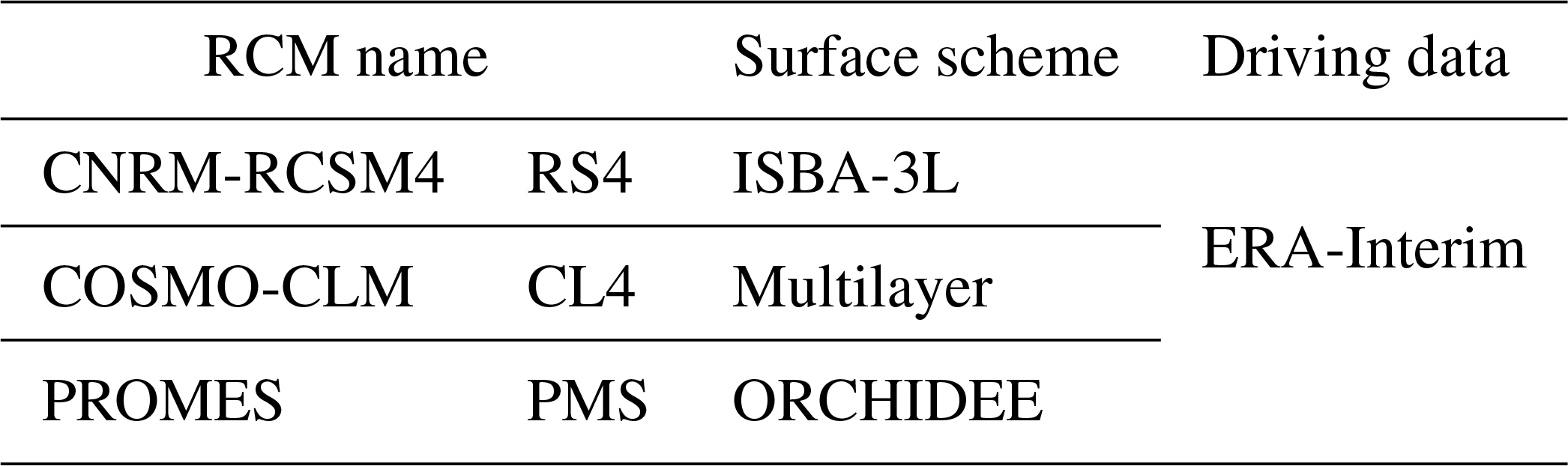
In this study, drought representation and propagation in three RCMs are analysed. RCM simulations were downloaded from the Med-CORDEX database, which is a contribution to the Coordinated Regional Climate Downscaling Experiment (CORDEX, Giorgi et al., 2009) focusing on the Mediterranean region (Ruti et al., 2016). The criterion used to select the models was that each one used a different surface scheme and therefore represented physical processes related to precipitation, soil moisture, and surface and sub-surface runoff in different ways. The three RCMs selected are listed in Table 1 and described below:

• The CNRM-RCSM4 (Sevault et al., 2014; Nabat et al., 2014) is a RCM developed by the CNRM. It includes the regional climatic atmospheric model “Aire Limitée Adaptation dynamique Développement InterNational” (ALADIN-Climate, Radu et al., 2008; Déqué and Somot, 2008; Farda et al., 2010; Colin et al., 2010; Herrmann et al., 2011), the three-layer version of the ISBA LSM (Noilhan and Planton, 1989; Noilhan and Mahfouf, 1996), the Total Runoff Integrating Pathways (TRIP) routing scheme (Decharme et al., 2010), and the regional ocean model NEMOMED8 (Beuvier et al., 2010). Hereafter, it will be referred to as RS4.

• The COSMO-CLM (CCLM) model (Rockel et al., 2008) is the climate version of the COSMO model developed by the Goethe Universität Frankfurt (GUF). The surface scheme is a multilayer version of the Jacobsen and Heise (1982) two-layer model. Hereafter, it will be referred to as CL4.

• The PROMES model (Castro et al., 1993; Sánchez et al., 2004; Domínguez et al., 2010) was developed by the Universidad Complutense de Madrid (UCM) and the Universidad de Castilla-La Mancha (UCLM). It is coupled to the ORCHIDEE LSM (De Rosnay and Polcher, 1998; Krinner et al., 2005). Hereafter, it will be referred to as PMS.

All of the RCM simulations are driven by the ECMWF Interim reanalysis (ERA-Interim) (Balsamo et al., 2012; Dee et al., 2011), which provides a global atmospheric reanalysis that starts in 1979 and is continuously updated in real time. In addition, it improves some important issues pertaining to ERA-40, such as the representation of the hydrological cycle. This reanalysis is performed by means of a data assimilation system based on a 2006 release of the ECMWF's Integrated Forecast System, IFS (Cy31r2), and uses a four-dimensional variational analysis (4D-Var) with a 12 h analysis window. The database has atmospheric and surface parameters with a temporal scale of 6 and 3 h, respectively. The spatial resolution is 80 km, with 60 vertical levels from the surface to 0.1 hPa.

ERA-Interim is a well-known atmospheric forcing used in a large number of studies. For instance, Belo-Pereira et al. (2011) and Quintana-Seguí et al. (2017) have validated it across the Iberian Peninsula. However, biases in this type of forcing have a negative effect on LSM simulations, which can be corrected (Ngo-Duc et al., 2005; Weedon et al., 2011).

In this study, ERA-Interim is the driving data of the three RCMs analysed. In addition, it is also used to force LSM simulations used as a reference in the soil moisture drought analysis. Hereafter, it will be referred to as ERA.

Table 1 RCMs analysed in this study.

3.2 Reference products

This section is divided into three subsections to describe the products used as reference data in the meteorological (Sect. 3.2.1), soil moisture (Sect. 3.2.2), and hydrological (Sect. 3.2.3) drought analyses. The products are listed in Table 2.

Table 2 Reference products used in the meteorological, soil moisture, and hydrological drought analyses.

3.2.1 Meteorological drought reference

SAFRAN is a meteorological analysis system (Durand et al., 1993, 1999) developed by Météo-France. It provides estimates of the following variables: precipitation, 2 m temperature, 10 m wind speed, 2 m relative humidity, and cloudiness, as well as modelled downward visible and infrared radiation following the radiation scheme of Ritter and Geleyn (1992). For this, an optimal interpolation algorithm (Gandin, 1966) that combines observations and a first guess is used. The first guess employed is ERA for all variables, except for precipitation, which is obtained from observations, and this is the reason why it has been selected as the reference dataset for the meteorological drought analysis. The meteorological station data belong to the Spanish Meteorological State Agency (Agencia Estatal de METeorología, AEMET) network. Precipitation is analysed by means of daily observations, whereas the remaining variables are analysed every 6 h. The data are then interpolated hourly using different methods that depend on the variable. In Spain, SAFRAN was extended for a 35-year period (1979/1980–2013/2014) (Quintana-Seguí et al., 2017) and was implemented and validated over the Ebro Basin (northeastern Spain) (Quintana-Seguí et al., 2016).

In this study, the standard version of SAFRAN, at a 5 km resolution, has been regridded to a 30 km resolution (Quintana-Seguí et al., 2019) to compare it with the RCM simulations as the reference in meteorological drought analysis and to force LSM simulations which are the reference in the soil moisture drought analysis. Hereafter, it will be referred to as SLR (SAFRAN low resolution).

3.2.2 Soil moisture drought reference

Offline LSM simulations are used in this study as a reference to analyse soil moisture drought because there is a lack of soil moisture data across mainland Spain that are suitable for studies that require a large spatial coverage. Internally, in RCMs, LSMs are bidirectionally coupled to the atmospheric model to simulate surface processes. However, when LSMs are run offline (forced by gridded databases), biases due to the atmospheric model and the coupling between the atmospheric model and the LSM are avoided. This makes offline LSM simulations good reference datasets to study drought. We selected three offline LSM simulations that use the same surface schemes employed by two of the RCMs analysed in this study.

The ISBA LSM (Noilhan and Planton, 1989; Noilhan and Mahfouf, 1996), developed by the CNRM, is composed of various modules that simulate heat and water transfer in the soil, vegetation, snow, and surface hydrology. This scheme has evolved using different approaches to model the soil. As a result, there are several versions that can be used. For this study, we selected the ISBA-3L (Boone et al., 1999), which considers a three-layered description of the soil. It should be stressed that the ISBA-3L is limited by certain aspects. For example, underground water is not represented, and there is no horizontal water transfer. Most of the ISBA's soil and vegetation parameters are derived from the ECOCLIMAP land cover database at a 1 km resolution (Masson et al., 2003; Kaptue et al., 2010; Faroux et al., 2013), such as the cover types and soil texture. This database considers more than 550 land cover types from all around the world. Its vegetation variability depends on the location, climate, and phenology.

The ORCHIDEE LSM (De Rosnay and Polcher, 1998; Krinner et al., 2005) was developed by the Institut Pierre-Simon Laplace (IPSL). It can be run in a stand-alone mode or coupled to the Laboratoire de Météorologie Dynamique (LMD-Z) general circulation model (Li, 1999), which was developed by the LMD in Paris. Hydrology is approached by means of a diffusive equation with a multilayer scheme. For this, the Fokker–Planck equation is solved considering a soil depth of 2 m distributed across 11 layers. The fine resolution is key to better model the interaction between the root profile and the soil moisture distribution at different depths as well as infiltration processes. In addition, ORCHIDEE includes sub-grid variability in soil moisture. Each grid box is divided into three soil moisture profiles with different vegetation distributions, but the same soil texture and structure that are obtained from the Zobler map (Post and Zobler, 2000).

In this study, three offline LSM simulations are used in the soil moisture drought analysis. Two of them use the three-layer version of the ISBA model (one simulation was forced with SLR and another one with ERA), and the other simulation uses the ORCHIDEE LSM forced with ERA. Hereafter, the ISBA and ORCHIDEE LSMs will be referred to as the ISB and ORC, respectively.

3.2.3 Hydrological drought reference

For the hydrological drought analysis, modelled and observed streamflow data were used as references. Two issues should be stressed before explaining these datasets. The first is that the Med-CORDEX database does not provide simulated streamflow for any of the three RCMs, which would be the variable ideally suited for this study. In the absence of such data, it was decided to use modelled total runoff (hereafter referred to as runoff) corresponding to the subbasins defined by a selection of gauging stations. We believe that this approximation is valid because we use a coarse time step, with a larger time propagation than the flow propagation. In fact, other studies use this variable to analyse hydrological drought (Vu et al., 2015; Meresa et al., 2016). The second issue is that Spanish basins are highly influenced by human management. However, RCMs do not simulate water management procedures but do simulate natural regime behaviour. Bearing these considerations in mind, only gauging stations satisfying the following criteria were considered:

1. A 95 % data completeness during the study period; this assures that the monthly series of observations has few gaps.

2. An area greater than 10 000 km²; the analysis was limited to large areas because streamflow is approximated by runoff, which is likely to perform poorly in small basins considering the coarse resolution of RCM simulations.

3. A KGE between SIMPA and the observations greater than 0.5 for the consideration of a near-natural regime. Stations had to be as natural as possible and their corresponding basins large enough to be compared to a low-resolution RCM. This is difficult in Spain due to the high degree of human influence. A high KGE value between SIMPA (naturalized flow) and the observations would indicate near-natural regime behaviour. Therefore, we performed a sensitivity analysis testing different values, and 0.5 was a reasonable compromise between the near-natural regime and a sufficient number of stations for the analysis. It is true that this threshold does not represent a completely natural regime, and thus some human influence can be present. However, it allows a fair comparison of the RCMs and observations.

The first criterion was satisfied by 87 stations, the second by 13 of the 87 stations, and the third by 8 of the 13 stations, which is the final selection. Figure 1 shows the locations of these stations as well as the relief and the river network. Tables 4, 5, and 6 contain their code, their area, and the basin to which they belong.

SIMPA is a Spanish acronym meaning “Integrated System for Rainfall–Runoff Modelling” (“Sistema Integrado de Modelización Precipitación-Aportación”) (Estrela and Quintas, 1996; Ruiz, 1999). It is a conceptually distributed hydrological model for water management developed by the Spanish Centre for Studies and Experimentation on Public Works (“Centro de Estudios y Experimentación de Obras Públicas”, CEDEX). SIMPA provides estimates of the water cycle's main components, such as precipitation, evapotranspiration, and river discharge, at a monthly scale in a natural regime. This regime is characterized by the free flowing of water, with no aspect unrelated to the environment (such as dams for water resource management) affecting it. Data are provided on a 1 km² grid. The model employs its own forcing, which uses an observational dataset similar to that of SAFRAN.

In this study SIMPA is used as a reference product for streamflow to analyse hydrological drought. Hereafter, it will be referred to as SMP.

Daily streamflow observations were also used as a reference in the hydrological drought analysis. These belong to the Spanish Ministry for the Ecological Transition, which provides data for basins comprising more than one region. Hereafter, they will be referred to as OBS.

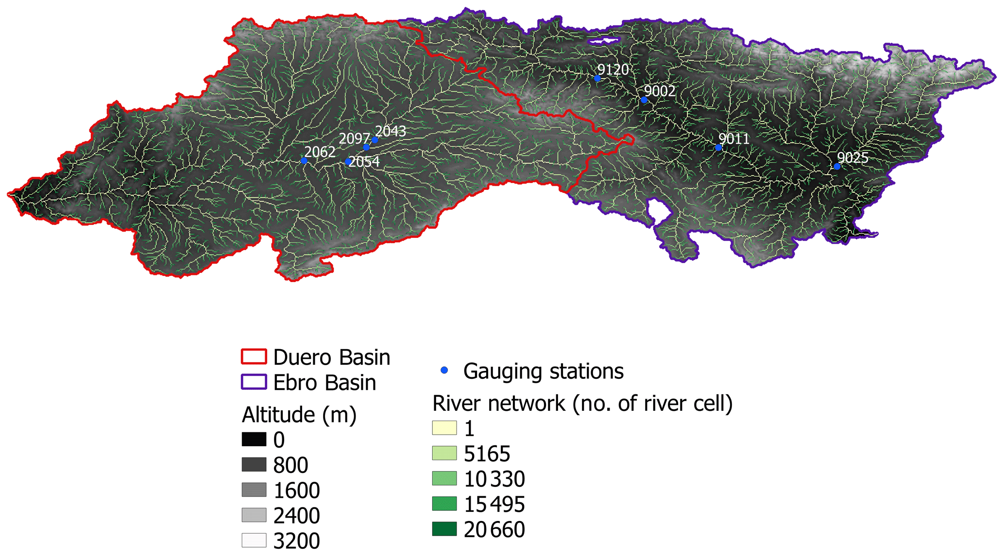
Figure 1 Map showing the relief, river network, and the locations of the gauging stations.

4 Methodology

The methodology employed in this study is the same as that used in Quintana-Seguí et al. (2019). Therefore, the two studies complement each other, providing a wider analysis of drought representation by both LSMs and RCMs.

Drought can be characterized in several ways. Here, we used standardized indices that define drought according to the variability in a given variable. It should be noted that variability is a key aspect of drought analysis. For the meteorological and soil moisture drought analyses, we computed the SPI and a standardized soil moisture index (SSMI) using precipitation and soil moisture data, respectively. For the hydrological drought analysis we computed two indices: the standardized streamflow index (SSI) using streamflow and the standardized runoff index (SRI) using total runoff.

4.1 Drought index calculation

We followed the spirit of the SPI to compute the SSMI, SSI, and SRI. In these indices, the variable's time series is transformed from its original distribution to a normal distribution. The resulting values correspond to the number of standard deviations by which the anomaly deviates from the mean. Biases were not computed, as they are zero by construction. The computation was carried out using monthly data for all indices. In the case of the SPI, a time series of the accumulated precipitation from the previous n months (with n being the index scale) was also calculated to perform the drought propagation analyses. It should be noted that in the SPI methodology, data are fitted to the corresponding parametric distribution, which can be an issue in studies that standardize several variables, as in our case. To solve this problem, we used the nonparametric methodology described by Farahmand and AghaKouchak (2015).

On the one hand, meteorological drought representation by RCMs was addressed by comparing their SPI-12 time series with those of ERA and SLR. Using results from an accumulation period of 12 months is particularly robust for seasonal reasons. In addition, this scale is suitable for the study area defined from a hydrological resource management perspective. Special attention was paid to differences in duration, severity, and area. In addition, the temporal correlation of the RCMs' SPI-12 with that of ERA and SLR was computed to identify regions where drought representation improved, if there were any. On the other hand, the analysis of the RCMs' soil moisture and hydrological drought representation was performed via the calculation of root-mean-square difference (RMSD) and the Pearson correlation coefficient (r) at a 95 % significance level of the standardized indices computed using an accumulation period of 1 month. We would like to stress that an RMSD equal to or greater than 0.5 often implies a change in drought category (i.e. from moderate to severe, for example) according to the SPI drought classification scale (McKee et al., 1993). To facilitate the Pearson correlation analysis interpretation, the guideline proposed by Evans (1996) was followed.

4.2 Meteorological drought propagation

The analysis of how meteorological drought propagates to soil moisture and hydrological drought is useful in hydrological resource management and allows for the detection of similarities and differences in the way models address the physical processes that drive this propagation. The methodology employed to analyse meteorological drought propagation is based on Barker et al. (2016). The soil moisture memory of precedent precipitation will vary from one point to another depending on the location because soil moisture is controlled by different aspects regarding climate and soil as well as vegetation properties such as precipitation, actual evapotranspiration, soil texture, stomatal resistance, and root depth, among others. To determine the month scale at which the precipitation deficit propagates to a soil moisture deficit, we carried out the following analysis:

• computed the standardized soil moisture index with a time accumulation of 1 month (SSMI-1);

• computed the SPI with a time accumulation of 1 to 28 months (SPI-n_x);

• identified the n_x scale that maximizes the correlation between SPI-n and SSMI-1.

The same methodology was employed to analyse how meteorological drought propagates to hydrological drought. For this, the SSI-1 and the SRI-1 were computed instead of the SSMI-1, and the SPI computation was performed using the areal mean of the basin precipitation defined by each studied gauging station.

4.3 Streamflow validation

The streamflow validation was carried out using the Kling–Gupta efficiency (KGE) (Gupta et al., 2009). The optimal KGE value is 1, whereas negative values are sign of a model's bad performance.

5 Results

First, meteorological drought representation by RCMs is evaluated (Sect. 5.1). Next, soil moisture drought representation by RCMs is analysed as well as how the models address the transition from meteorological to soil moisture drought (Sect. 5.2). Finally, hydrological drought representation by RCMs and the propagation of meteorological to hydrological drought are analysed (Sect. 5.3).

5.1 Meteorological drought

In this section, we will focus on precipitation because its decrease or absence are the main cause of meteorological drought. The SPI is computed for the RCMs, ERA (driving data), and SLR (reference dataset). On the one hand, the comparison of the RCMs' SPI with that of ERA allows us to identify and determine the extent to which these models reproduce the structures of their driving data. On the other hand, the comparison of the RCMs' and SLR's SPI shows the extent to which the RCMs improve these structures, as the SLR dataset is based on observations.

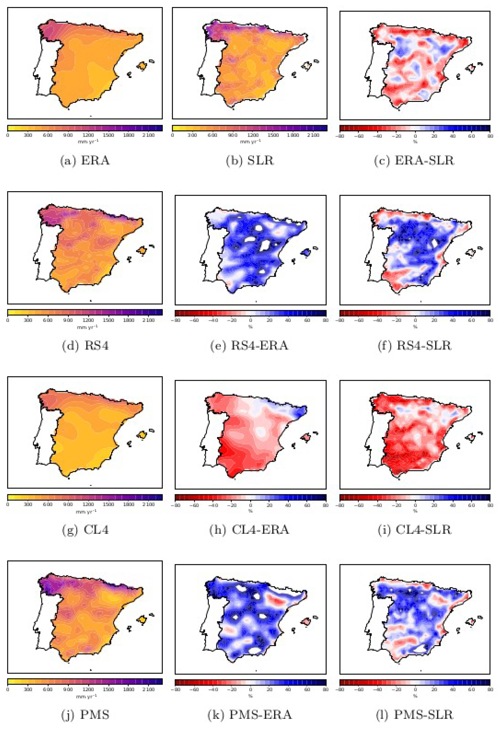
Figure 2 Mean annual precipitation across the study area from 1989 to 2008: ERA (a), SLR (b), RS4 (d), CL4 (g), and PMS (j). Panel (c) shows the difference between ERA and SLR mean annual precipitation; panels (e), (h), and (k) show the difference between the RCMs and ERA mean annual precipitation; and panels (f), (i), and (l) show the difference between the RCMs and SLR mean annual precipitation.

5.1.1 Mean annual precipitation comparison

Figure 2a–c shows the mean annual precipitation of ERA and SLR as well as the difference in mean annual precipitation between them. Figure 2d–l shows the RCMs' mean annual precipitation and their difference with respect to ERA (Fig. 2e, h, k) and SLR (Fig. 2f, i, l). All products show greater precipitation in the northwestern and northern regions of the peninsula (exceeding 2000 mm yr⁻¹) as well as over mountainous chains. The products also show that precipitation is lower along the main basin valleys (due to the orographic shadow effect) and minimal over the southeast, which is the driest region of the peninsula. For instance, precipitation across some areas of this region does not exceed 100 mm yr⁻¹. The RCMs' mean precipitation spatial structures show similar behaviour to those from ERA and SLR. The fact that precipitation is high over mountainous chains indicates the strong influence of relief, which is key in the way water from precipitation is distributed. In fact, we would like to stress SLR's significant contrast in relief due to its use of data from AEMET's dense pluviometric network. This evidence indicates the complex spatial structure of precipitation in Spain.

Regarding the RCMs, RS4 and PMS show the greatest similarity and the highest contrast with CL4. When compared to ERA, both RCMs have higher precipitation, especially in mountainous areas. Modelled precipitation tends to overestimate precipitation compared with observations and ERA (Sylla et al., 2010). This reflects the addition of water in the form of precipitation, improving the RCMs' spatial distribution of precipitation with respect to the driving data. However, when RS4 and PMS are compared to SLR, precipitation is underestimated over some areas (valleys and the coastline). It must be noted that SAFRAN is mainly based on rain gauge information. The CL4 model is a different matter, as it underestimates precipitation for almost all of Spain when compared with ERA and SLR.

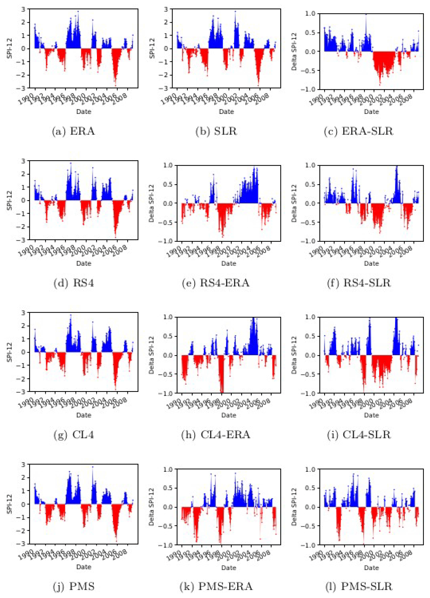
Figure 3 SPI-12 time series calculated with the spatially averaged time series of mainland Spain precipitation, as reproduced by ERA (a), SLR (b), RS4 (d), CL4 (g), and PMS (j). Panel (c) shows the difference between ERA and SLR SPI-12; panels (e), (h), and (k) show the difference between the RCMs and ERA SPI-12; and panels (f), (i), and (l) show the difference between the RCMs and SLR SPI-12.

5.1.2 SPI comparison

Once the spatial distribution of precipitation in the peninsula is described, we can study the variability in the different products and thus their capacity to reproduce drought spells.

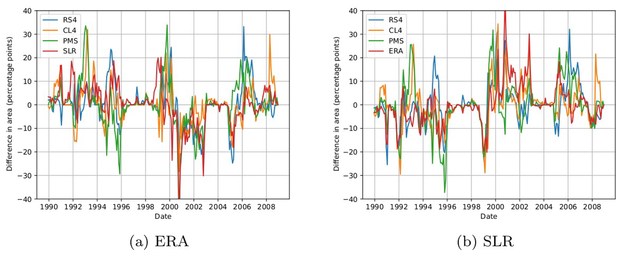
Figure 4 Differences in the proportion of area under drought (SPI-12 $<-\mathrm{1}$) estimated by (i) the RCMs and SLR with respect to ERA (a) and (ii) the RCMs and ERA with respect to SLR (b).

Figure 3 shows the time series of the SPI-12 calculated using mainland Spain's average precipitation as reproduced by ERA (panel a), SLR (panel b), and the RCMs (panels d, g, and j). The computation is performed for a time accumulation of 12 months. ERA and SLR show several drought spells which occurred during the 20 years that comprise the study period (the most severe occurred in 2005–2006). These spells coincide with those found by Belo-Pereira et al. (2011) and also appear in the RCMs' SPI time series plots. Therefore, RCMs are capable of reproducing these spells. However, differences in duration and severity can be observed. For instance, the duration of the spell that occurred in 1992 and 1993 was 21 and 22 months according to CL4 and PMS, respectively. However, it lasted 19 and 17 months according to SLR and ERA, respectively. Another interesting result is found in the spell that took place in 2002. CL4's mean severity is similar to that of ERA. However, the mean severity of both RS4 and PMS is in better agreement with that of SLR than with their driving data. Other information that can be extracted from these results is the timing of drought between the RCMs and their driving data and reference data. For example, the RCMs, ERA, and SLR agree that the spell that occurred between 1994 and 1995 started in May 1994. RS4, CL4, ERA, and SLR agree that it ended in December 1995, but the PMS model indicates the end of the spell occurring a month before the rest (November 1995). The spell between 2004 and 2006 started in November 2004 according to SLR, ERA, and PMS, which show similar durations (ERA shows 23 months, and SLR and CL4 show 24 months). However, it started in January 2005 according to RS4 and CL4 and had a longer duration: 27 (RS4) and 25 (CL4) months. In a previous study, a spurious trend in ERA was detected (Quintana-Seguí et al., 2019). This can be observed in Fig. 3c, where the difference between the SPI-12 time series of ERA and SLR is represented. However, the differences between the RCMs and SLR SPI-12 time series show that these models do not drag this trend.

Figure 5 Map of the temporal correlation (Pearson) between the SPI-12 time series produced by (i) the RCMs and SLR with respect to ERA (a) and (ii) the RCMs and ERA with respect to SLR (b). Portugal and regions from the study area (mainland Spain) whose values are not within the colour scale are represented in white.

To deepen the analysis of the spatial structure of meteorological drought, monthly SPI-12 maps were computed. The comparison of these structures, as shown by the RCMs, with those of their driving data and the reference dataset, provides more information about drought representation by RCMs. For instance, the temporal evolution of the spatial correlation of the SPI-12 maps of the RCMs with ERA and SLR (not shown) indicates the similarity between the RCMs and their driving data and reality (as approximated by SLR), respectively. In the first case, RS4 most resembles ERA. Despite not showing the highest correlations, it has less variability and is therefore more robust. The correlations of CL4 and PMS with ERA are more variable, reaching values close to zero in some months, in which the spatial structure of drought is not captured. In the second case, RCMs show worse correlation with SLR than with ERA, as expected. It should be stressed that RS4 also displays better correlations than the other RCMs when these are compared with SLR. Thus, out of the three RCMs studied, RS4 deviates less from the driving data and most resembles the reference. The correlation between ERA and SLR shows some variability in its temporal evolution, especially since 2000. This is likely due to the effect of the spurious trend identified in Fig. 3. To complement the spatial structure analysis, Fig. 4 provides information about the difference in the percentage of the area affected by drought (SPI-12 $<-\mathrm{1}$) between the RCMs and (i) ERA (panel a) and (ii) SLR (panel b). The differences are generally under 25 %. In general, the RCMs show similar behaviour during a drought spell, meaning that they all overestimate or underestimate the affected area. For example, all three underestimate the area in 1994, overestimate it in 1995, and underestimate it in 1996. The difference relates to the degree to which they deviate. On the one hand, in 1995, RS4 overestimates the percentage of area affected by drought by 20 %, CL4 by approximately 15 %, and PMS by less than 10 %. On the other hand, in 1996, PMS underestimates this percentage by more than 30 %, while RS4 and CL4 underestimate it by 10 %. Another example is how the RCMs overestimate the area in 2000 and how they underestimate it between 2001 and 2003. RS4 is the RCM that shows the lowest percentage difference, which is consistent with our previous results.

Finally, Fig. 5 provides an idea of the spatial structures of drought representation. For this, the temporal correlation (Pearson) of the SPI-12 between the RCMs and (i) ERA (maps from Fig. 5a) and (ii) SLR (maps from Fig. 5b) is computed for each grid point. The correlations of the RCMs with ERA are above 0.8 in the south and worsen towards the north and the eastern coast, reaching 0.2. The Ebro Basin is the region showing the poorest values and thus the largest differences in drought representation between the RCMs and ERA. Differences in this area are also identified in the map showing the correlation between ERA and SLR, where values are even negative. However, when the RCMs are compared with SLR (Fig. 5b), the correlations are higher across this basin. Consequently, RCMs improve drought representation across this region.

5.2 Soil moisture drought

This section analyses how RCMs reproduce soil moisture drought (Sect. 5.2.1) and its propagation from precipitation to soil moisture (Sect. 5.2.2). Offline LSM simulations from the ISBA-3L and ORCHIDEE are used as references. We should bear in mind that in these simulations, soil processes do not impact the atmosphere, whereas the RCM simulations are performed in coupled mode and thus interact with the atmosphere.

5.2.1 SSMI comparison

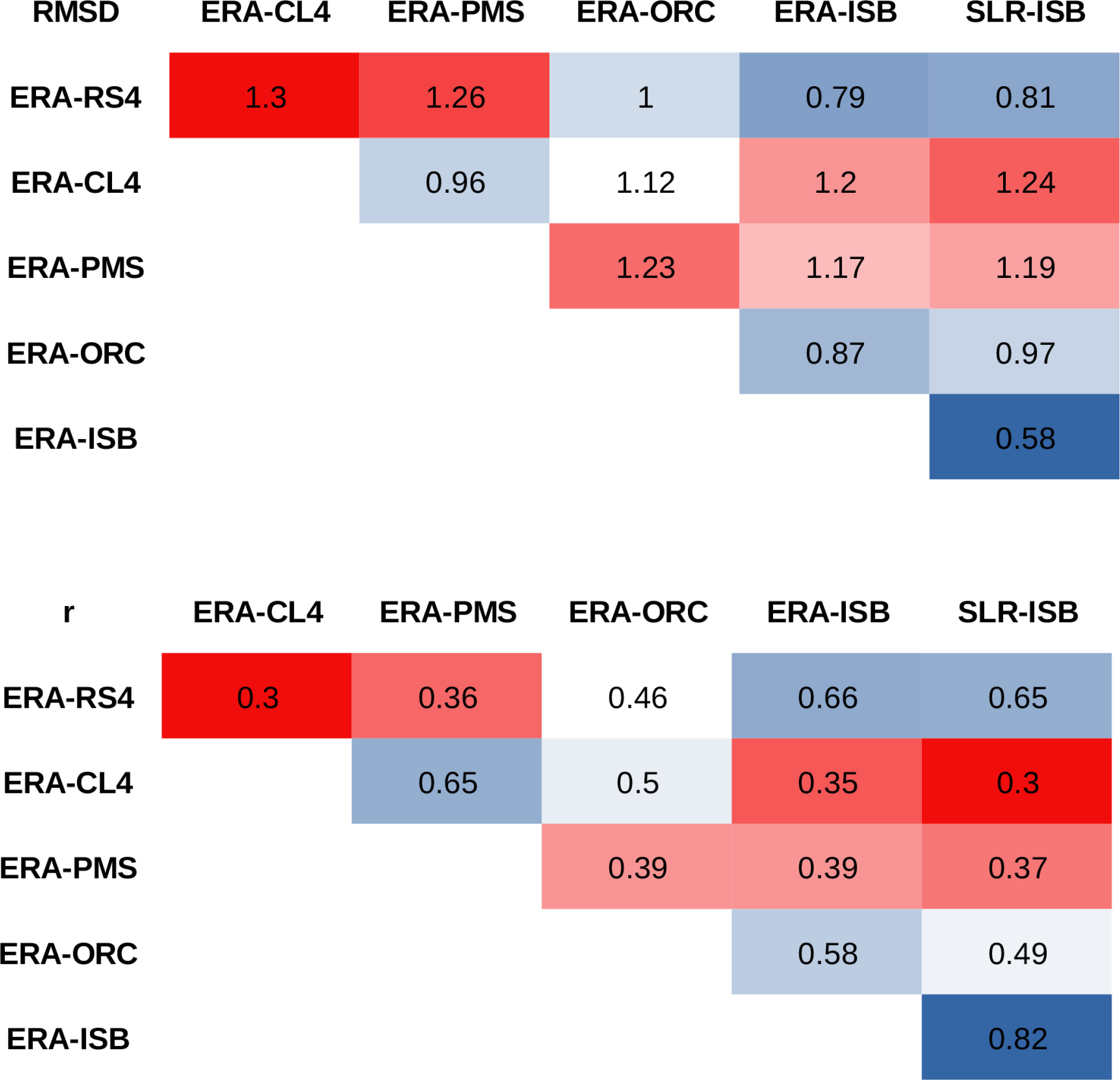
The RMSD and the Pearson correlation coefficient (r) are calculated by comparing the SSMI from the RCM simulations and the LSM simulations. All mesh points and time steps are included in the comparison. Therefore, the results provide information regarding spatial and temporal drought structures. It should be noted that biases are not calculated because they are zero by construction (the mean of the SSMI is zero). The results are shown in Table 3, the upper block of the table corresponds to the RMSD and the lower block corresponds to the r calculations. A colour scale consisting of a blue (largest similarity between models) to red (lowest similarity between models) gradient via white has been included to facilitate reading.

To put these results into context, we will consider the drought classification according to the SPI, which is divided into eight categories from “extremely wet” (SPI =2) to “extreme drought” (SPI $=-\mathrm{2}$). A RMSD equal to 1 is a standard deviation of the index studied (in this case, the SSMI). In the framework of drought analysis, a value higher than 0.5 would imply a change in category (for example, from “slightly wet” to “moderately dry”). Therefore, the upper block of Table 3 shows that there is a change in drought category when comparing the RCMs with the reference offline LSM simulations, as the RMSD is above 0.5 (fourth to sixth columns). In addition, the three RCMs compared among them also represent soil moisture droughts of different categories (second and third columns), as expected.

Going into detail, we can observe some similarity between the RS4 simulation, which uses the ISBA surface scheme, and the ISB simulations. Compared with ISB, RS4 reproduces drought better than the other RCMs used in this study. However, this does not occur when the PMS and ORC simulations are compared, despite using the same surface scheme. In fact, RS4 and CL4 are, in general, more similar to ORC than PMS, according to the statistics. The SSMI comparison of the RCMs with both ISB simulations (fifth column vs. sixth column) shows very similar statistics. Discrepancies could be explained by the RCMs' land–atmosphere coupling and forcing effects.

Table 3 Comparison of the SSMI data from the RCM and LSM simulations. The upper block shows the RMSD, and the lower block shows the Pearson correlation (r). The colour scale is a gradient from blue (largest similarity between models) to red (lowest similarity between models) via white.

5.2.2 Propagation to soil moisture drought

n_x maps from Fig. 6 indicate the scale in months at which the correlation between the SSMI-1 and SPI-n is maximal and thus the temporal scale at which meteorological drought propagates to soil moisture drought. Figure 6a–c shows RCM maps, whereas Fig. 6d–f shows ISB and ORC LSM (reference data) maps. The scale ranges from 0 to 28 months, with the dynamics of the model in regions with a yellowish tone being slower than those in regions with a bluish tone.

Figure 6a–c shows that the RCMs provide different results even though they use the same driving data, which indicates the predominance of model structure with respect to the driving data. This becomes more evident when a RCM is compared to the LSM that has the same surface scheme. For example, the RS4 and ISB (Fig. 6a, d, and e) maps show similar spatial patterns. These are very homogeneous, with scales that range from 1 to 4 months, implying that ISB reacts very quickly to precipitation. Another example is the comparison between PMS and ORC (Fig. 6c and f). Both models show greater heterogeneity than ISB, with scales from 1 to 20 (PMS) and 24 (ORC) months, highlighting the role of the continental surface. Finally, the CL4 (Fig. 6b) behaviour is quite homogeneous. The peninsula is divided into two areas, one over the northwest, where the n_x scale ranges between 6 and 12 months, and a larger one with a fixed value of 20 months. It is interesting to note the similar spatial structures from the ERA-CL4 and ERA-ISB maps (Fig. 6b and e), indicating that soil moisture drought propagation by CL4 drags the same spatial structures as its driving data.

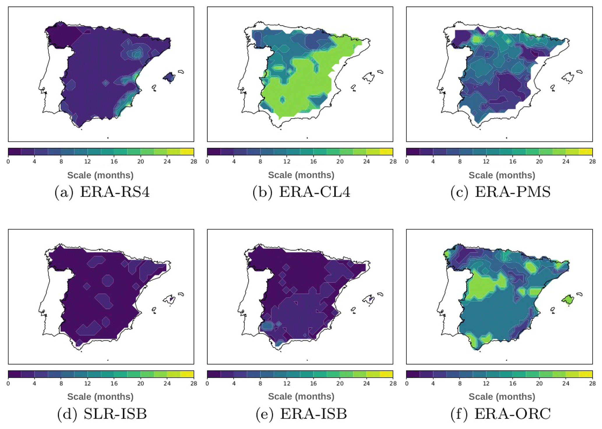
Figure 6 The n_x timescale maximizing the correlation between the SPI-n_x and SSMI-1 for the RCM and LSM simulations. Portugal and regions from the study area (mainland Spain) whose values are not within the colour scale are represented in white.

5.3 Hydrological drought

In Sect. 5.3.1, streamflow and aggregated runoff will be compared. Next, the RCMs' capacity to simulate hydrological drought will be analysed by comparing the SSI and SRI (Sect. 5.3.2). Finally, we will analyse the way in which RCMs reproduce meteorological drought propagation to hydrological drought (Sect. 5.3.3).

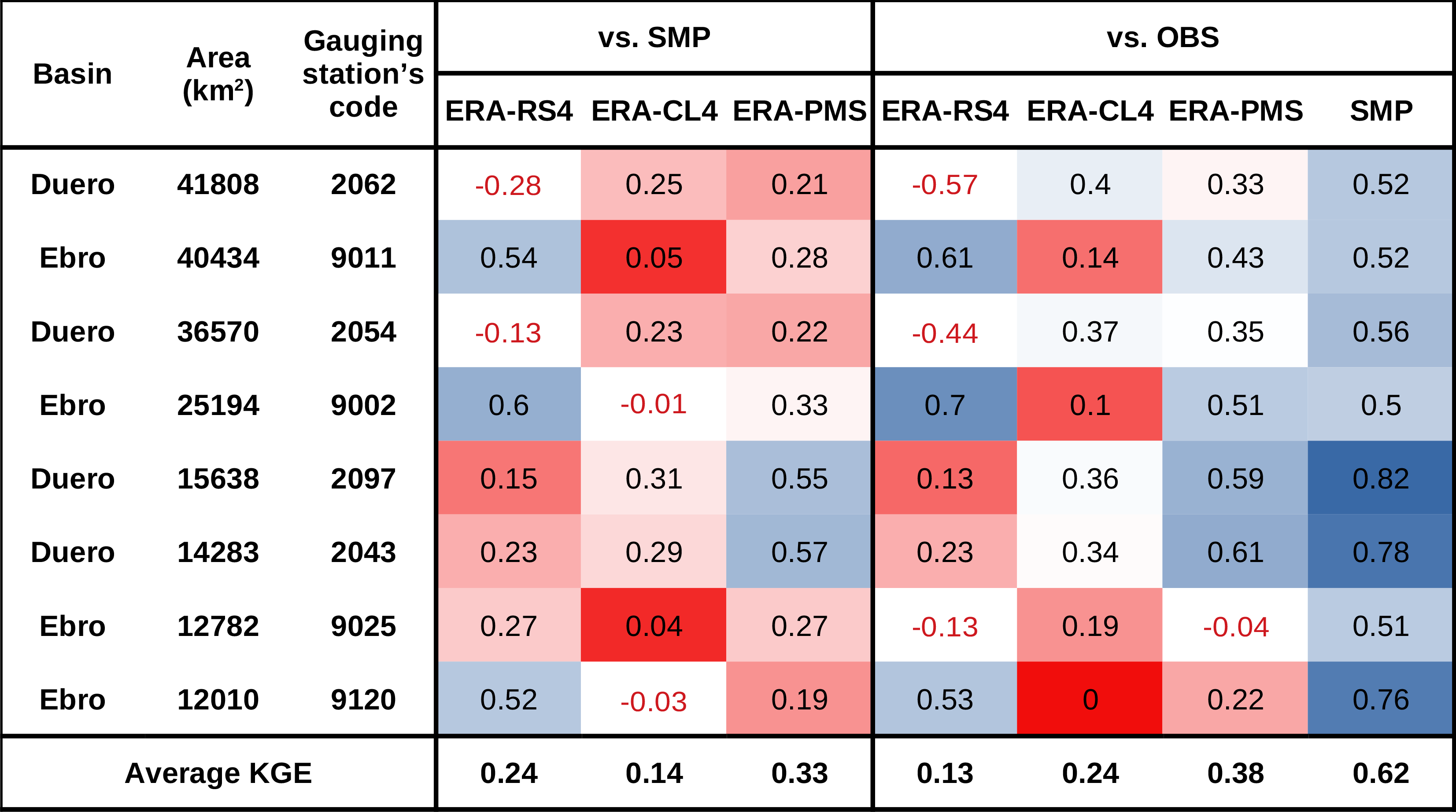
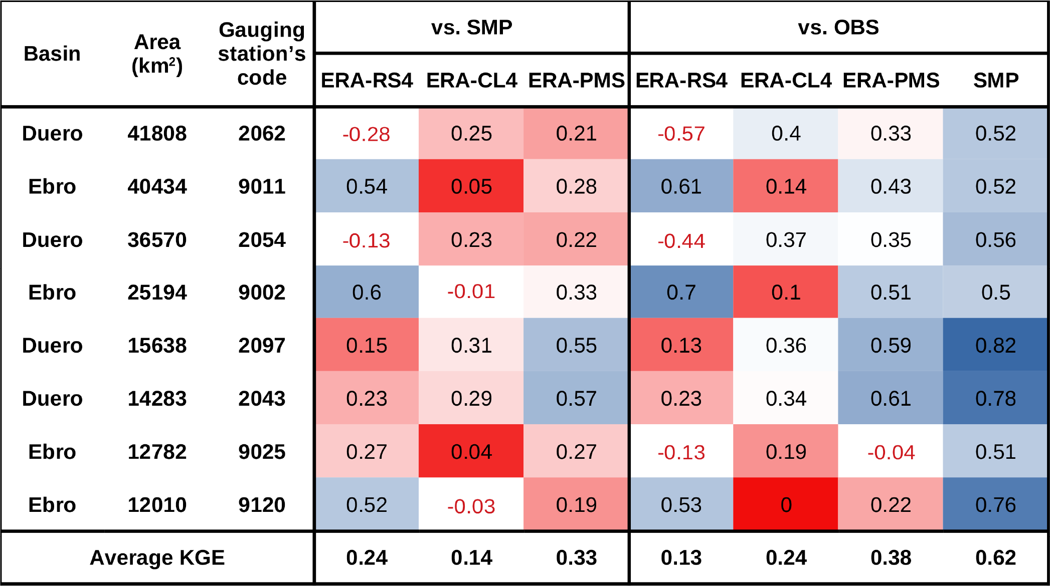
Table 4 KGE of the aggregated runoff simulated by the RCMs compared with the reference streamflow of the SMP model and OBS. Note that observations are affected by anthropic effects. Negative values (model's poor performance) are shown in red. The colour scale only displays positive KGE values, and consists of a blue (best performance between the RCMs and SMP or OBS) to red (worst performance between the RCMs and SMP or OBS) gradient via white. The bottom row shows the average KGE for each RCM.

5.3.1 Streamflow and aggregated runoff comparison

Table 4 shows the KGE comparing RCM aggregated runoff with SMP and OBS as well as the comparison between SMP and OBS. All of these comparisons are performed at a monthly scale. Negative values, indicating poor performance, are marked in red. For the positive KGE values, a colour scale consisting of a blue (best performance between the RCMs and SMP or OBS) to red (worst performance between the RCMs and SMP or OBS) gradient via white has been included to facilitate reading.

The RCMs show KGE values that are negative or close to zero at many stations. Focusing on the positive KGE values, CL4 has the worst performance, as the values are below 0.5. Although RS4 is the RCM showing the highest KGE value (0.7 at station number 9002 for the comparison between RS4 and OBS), PMS performs better across both basins according to the average value (bottom row of Table 4).

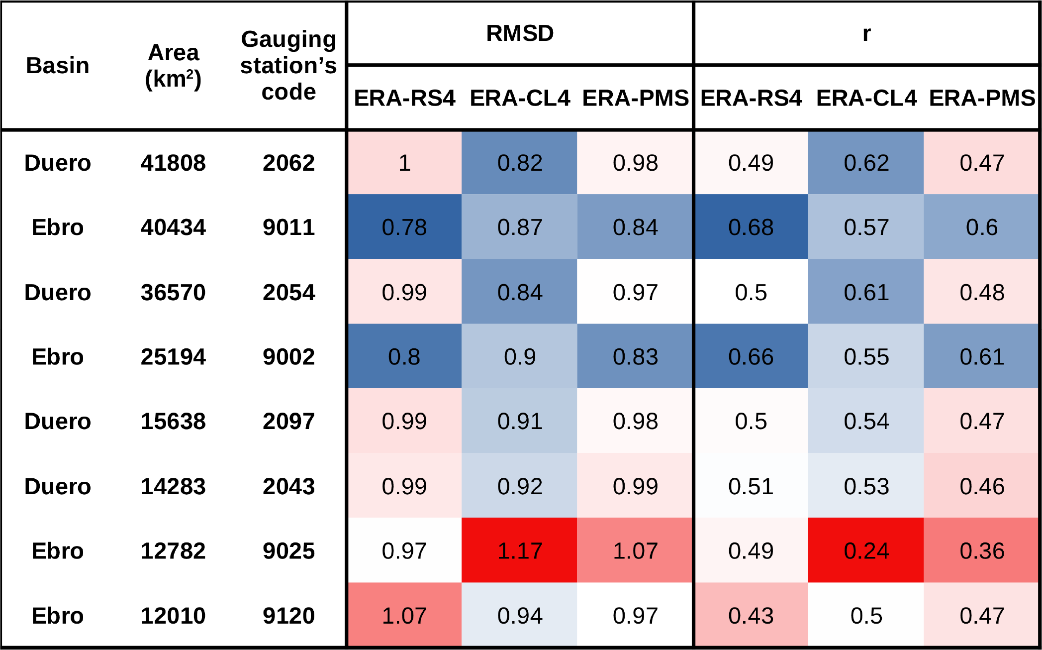
Table 5 Comparison of the SRI from the RCMs with the SSI from SMP. The table shows the RMSD and the Pearson correlation (r). The colour scale is a gradient from blue (largest similarity between models) to red (lowest similarity between models) via white.

An analysis comparing the temporal series (not shown) of the RCMs' aggregated runoff with the reference streamflow (SMP and OBS) shows that CL4 sustains summer flows, which is a positive aspect. This is not the case for RS4 and PMS, which have steeper recession curves. In addition, RS4 is found to overestimate streamflow peaks at stations in the Duero Basin. Finally, we would like to note that RS4 and PMS show a different behaviour from that of the reference data at station number 9025 (which represents the Segre subbasin). Both models overestimate a large number of peaks. We believe that this may be explained by the fact that the Segre subbasin is nival.

5.3.2 SSI and SRI comparison

Table 5 shows the RMSD and the Pearson correlation coefficient, r, comparing the RCMs' SRI with SMP's SSI. A colour scale consisting of a blue (largest similarity between models) to red (lowest similarity between models) gradient via white has been included to facilitate reading.

The results are similar to those in Sect. 5.2.1, as the RMSD values are above 0.5 (which often indicates a change in drought category). Therefore, according to the SPI drought classification, the RCMs represent hydrological droughts of a different category from that of the reference dataset. Nevertheless, the RCMs show moderate positive correlations with SMP according to the guideline proposed by Evans (1996). We would like to note that the worst statistics are shown by station 9025, which is identified in the previous section as the station showing the worst performance. It is highly influenced by the effects of snow, which could explain the high RMSD and weak r values.

5.3.3 Propagation to hydrological drought

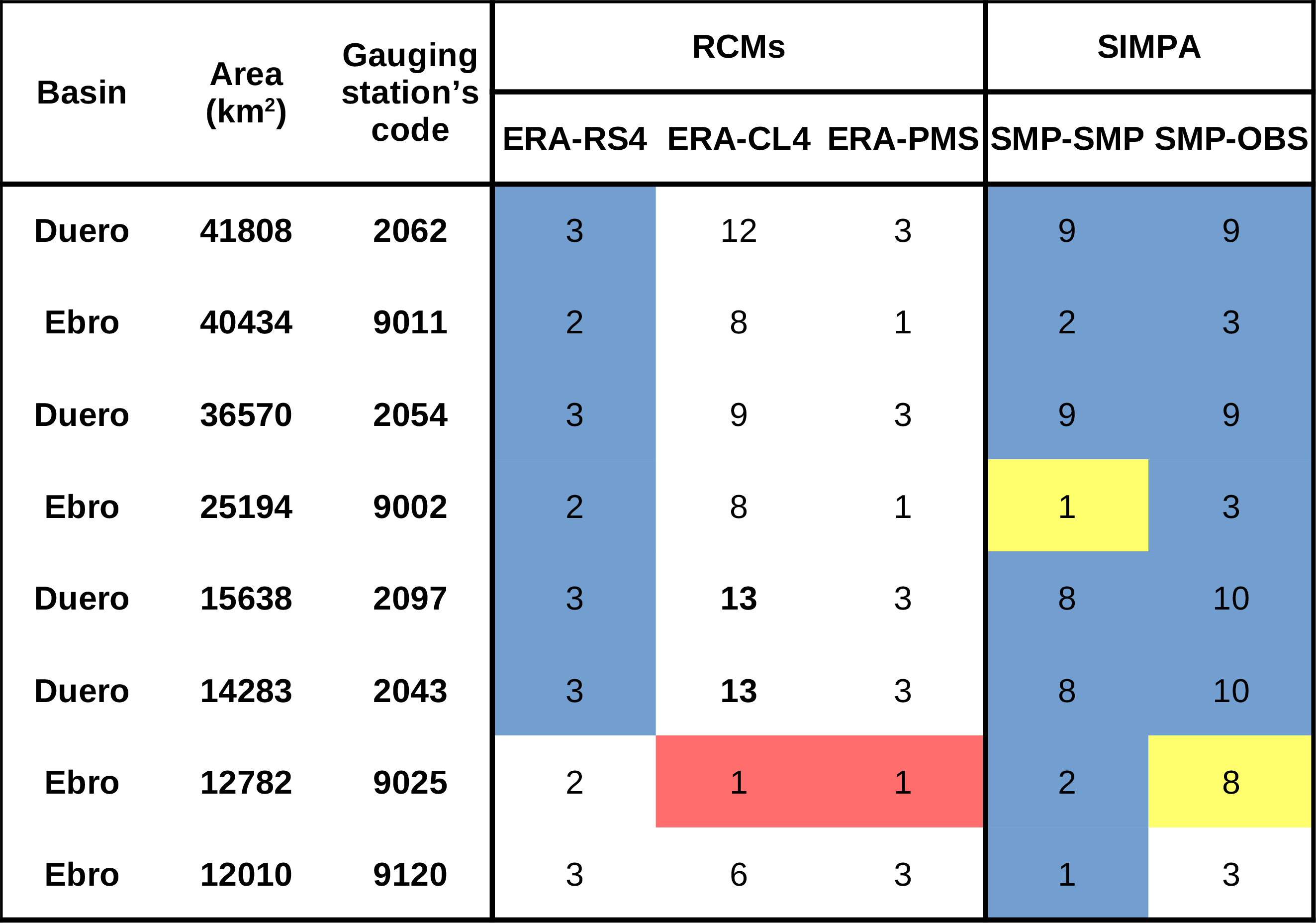
Table 6 shows the n_x values that indicate the monthly scale at which the correlation between the SPI-n_x and (i) SRI-1 (RCMs) and (ii) SSI-1 (SMP and OBS) is maximal. This can be interpreted as the temporal scale at which meteorological drought propagates to hydrological drought. To better understand these results and the extent to which they reflect the propagation of a precipitation anomaly to a streamflow anomaly, a colour scale is included to indicate the strength of the correlation. It follows the guideline given by Evans (1996): very strong (yellow), strong (blue), moderate (white), and weak (red).

In contrast to Sect. 5.2.2, RS4 and PMS show very similar scales: means of 3 months for stations in the Duero Basin and 2 months (RS4) and 1 month (PMS) for stations in the Ebro Basin. However, CL4 provides larger scales, from 9 to 13 months (Duero Basin) and from 1 to 8 months (Ebro Basin). The difference in scales shown by the RCMs is an indicator of the relevance of model structure in drought propagation. This result is also obtained in Sect. 5.2.2.

The RCMs and SMP show higher n_x values and thus slower dynamics in the Duero Basin than in the Ebro Basin. This is in agreement with the n_x values obtained using the SSI-1 computed with OBS, in which the mean n_x values are 9 (Duero) and 4 (Ebro). Analysing these results, we can establish that the RS4 and PMS runoff responds quickly to precipitation anomalies. When compared to SMP and OBS, the monthly scales provided are in good agreement in the Ebro Basin but are too low in the Duero Basin. In contrast, CL4 shows larger scales and behaves inversely to RS4 and PMS, as it is in better agreement with SMP and OBS in the Duero Basin.

Focusing on the strength of the correlations, RS4 (coupled to ISB) shows strong positive correlations at six of the eight stations analysed, indicating that precipitation has a significant role in streamflow variability. However, the correlations of CL4 and PMS with the SPI-n_x are moderate (even weak for station number 9025), which implies that there are also other factors driving this variability.

Table 6 The n_x timescale maximizing the correlation between the SPI-n_x and (i) SRI-1 (RCMs) and (ii) SSI-1 (SMP and OBS). Scales longer than 12 months are marked in bold. A colour scale has been included to indicate the strength of the correlations between the SPI-n_x and (i) SRI-1 and (ii) SSI-1 following the guide proposed by Evans (1996). The correlation ranges and the associated colours are as follows: (i) very strong, 0.80–1.0 (yellow); (ii) strong, 0.60–0.79 (blue); (iii) moderate, 0.40-0.59 (white); and (iv) weak, 0.20–0.39 (red).

6 Discussion

This study provides an assessment of how RCMs represent meteorological, soil moisture, and hydrological drought as well as the way in which precipitation anomalies propagate to soil moisture and streamflow anomalies. This assessment was performed using standardized indices, which we believe are a good option for performing drought analysis. The reason for this is that they describe drought based on the variability in a given variable; thus, each type of drought can be studied using the variable that best suits its characteristics. In this work, four indices were computed: SPI (precipitation), SSMI (soil moisture), SSI (streamflow), and SRI (total runoff).

RCMs provide a good representation of meteorological drought. The results show that they are capable of reproducing the same drought spells as those detected by their driving data and the reference data. However, they differ in terms of an event's duration, severity, and area, as expected. We have identified that RCMs improve drought representation with respect to the driving data in several aspects. For instance, the temporal evolution of the SPI-12 shows that the severity of some of the drought spells is closer to that of the reference data. In addition, they do not reproduce the spurious trend identified in the driving data, which could lead to a misrepresentation of the phenomenon. Finally, a temporal correlation analysis shows that drought representation is improved over the northeastern region of the Iberian Peninsula, which is a known limitation of global analysis across Spain. These results are consistent with previous studies showing that RCMs provide a suitable representation of drought using drought indices across Spain (Barrera-Escoda et al., 2013; Maule et al., 2013; García-Valdecasas Ojeda et al., 2017).

Unlike the previous analysis, the results regarding soil moisture and hydrological drought representation show differences when RCMs are compared among themselves and to the reference data. The analyses are carried out using the RMSD and Pearson correlations, and the observed uncertainty corresponds, in most cases, to a change in the drought category (according to the SPI drought classification) of RCMs with respect to the reference data. These differences are expected if we consider the following aspects:

• First, the reference data that are employed. LSM offline simulations are used as reference datasets for soil moisture drought analysis due to the lack of observations. In Spain, soil moisture data from the REMEDHUS network (Martínez-Fernández et al., 2013) and the Valencia Anchor Station (Coll-Pajarón, 2017) are available. However, these datasets are suitable for studies in which large spatial coverage is not an issue (such as model or satellite-derived data validation), which does not apply to our case. Remote sensing products could also be an option, but there are certain limitations that should be taken into account, for example, uncertainty sources, gaps in the data, and short time series (AghaKouchak et al., 2015). Escorihuela and Quintana-Seguí (2016) showed that different satellite products behave differently across a region representative of Mediterranean landscapes (Catalonia in the northeast Iberian Peninsula). Therefore, using these products would add more uncertainty to the study. In addition, the retrieved soil moisture data correspond to surface soil moisture, and, in this study, we considered root zone soil moisture. If the study was limited to the consideration of surface soil moisture, processes important to soil moisture drought would not be considered. Nevertheless, improvements in this discipline, as well as an increase in the length of time series, will convert these products into interesting alternatives for LSM simulations. Regarding the hydrological drought analysis, the observed streamflow in mainland Spain was used as a reference. However, the large number of dams and canals have a high anthropic impact on river systems, affecting the observed streamflow. As RCMs do not take these effects into account, a simulation from the SIMPA model that provides streamflow data considering a natural regime is necessary as a reference dataset. It would be interesting to include these effects in RCM modelling to perform drought analysis using the observed streamflow as reference data. This would provide an idea of the anthropic impact on hydrological drought.

• The second consideration is the use of LSMs. In this study offline LSM simulations are used as reference datasets to compare with the RCM simulated soil moisture, due to the lack of observed soil moisture data. This is natural as RCMs internally used a LSM coupled to the atmosphere. We used three simulations as references, instead of one, because LSMs vary from one to another in several important aspects, such as soil discretization, evapotranspiration formulation, runoff formulation, subgrid processes, and so on. All of these differences impact soil moisture (Koster et al., 2009) and streamflow.

• Third, the use of simulated total runoff to compute the SRI is due to the lack of RCM modelled streamflow data to compute the SSI. Hydrological drought representation and propagation are likely to be affected by this approximation according to the KGE values shown in Sect. 5.3.1. When compared to SMP, the KGE using total runoff is under 0.25 in almost half of the cases, which indicates poor performance. However, we would like to stress that PMS is the RCM that best approximates streamflow according to the KGE values.

• Finally, the effects of RCM coupling with the atmosphere should be taken into account, as the soil moisture references are LSM simulations performed in an uncoupled mode and thus do not include atmospheric feedback.

We would also like to note the relevance of the timescale used to compute drought indices. According to García-Valdecasas Ojeda et al. (2017) and Bowden et al. (2016), the added value of the SPI is influenced by the accumulation period employed. This is interesting to consider because soil moisture and hydrological droughts have different scales of propagation, and differences are also found in the propagation analysis in Sect. 5.2.2 and 5.3.3.

The main objectives of this study are to evaluate drought properties and propagation in RCM simulations. At this point, we would like to mention uncertainty, which is an important issue in this kind of study. Although the analysis was performed using only three models, these models provide different results in terms of drought indices and, especially, drought propagation. Adding more models would show the spread with more detail, but we believe that the differences among the three models are large enough to show that RCM developers should look at these issues and that RCM users should take them into account.

A key result of the study is the relevance of the models' physics, which prevails over the driving data. This is shown in the soil moisture and hydrological drought representation evaluation as well as in the analyses of drought propagation. In the latter case, the model's structure influences the temporal scale at which the variability in precipitation affects that of soil moisture and streamflow. For instance, in the analysis in Sect. 5.2.2, the spatial patterns of RS4 (coupled to ISB) and ISB are very similar and show that ISB, and thus RS4, respond too quickly to precipitation. The spatial structures of PMS (coupled to ORC) and ORC differ to a greater extent. The temporal scale of PMS is shorter than that of ORC, which may be due to coupling effects and to the fact that the precipitation extremes in PMS are too strong (Domínguez et al., 2013). Wang et al. (2011), in their analysis of climate change impacts on droughts, also highlight the fact that model structure is likely to contribute in an extensive way to different regional climate change projections.

The results obtained are coherent with those from Quintana-Seguí et al. (2019), in which the soil moisture and hydrological drought analyses also showed differences among LSMs. Therefore, both studies provide clear proof that improvements in modelling concerning soil moisture and streamflow are needed.

7 Conclusions

In the context of a changing climate, it is necessary to evaluate the evolution of extremes, such as drought. Understanding the processes involved is therefore vital. To do so, the current modelling tools must first be evaluated. The work presented here analyses how RCMs represent meteorological, soil moisture, and hydrological drought and the propagation from a precipitation anomaly to soil moisture and streamflow anomalies.

Of the three RCMs analysed, RS4 shows the largest similarities with the reference data and deviates the least from its driving data in the meteorological and soil moisture drought representation analyses. However, none of the RCMs analysed can be clearly identified as showing the best performance with respect to hydrological drought representation. CL4 and RS4 show larger similarities with the reference data than the other RCMs across the Duero and Ebro basins, respectively. The propagation to soil moisture drought analysis indicates that RS4 reacts too quickly to precipitation anomalies, while PMS provides richer spatial patterns and a higher role of the continental surface. Finally, the propagation to hydrological drought analysis shows that RS4 and PMS react quickly to precipitation anomalies. These RCMs are in better agreement with the reference data than CL4 over the Ebro Basin, whereas CL4 is in better agreement with the reference data over the Duero Basin.

It is concluded that RCMs provide added value to meteorological drought representation, minimizing possible error sources from the driving data and ameliorating its characterization over areas that are known to pose certain problems to global driving data products. However, soil moisture and hydrological drought representation by RCMs show uncertainties. This is mainly due to the relevance of model physics and its prevalence to the driving data. Similar results were obtained for the propagation processes, in which model structure was found to influence the dynamics of drought propagation, showing different temporal scales depending on how precipitation variability is formulated within the model.

RCMs are a suitable tool for meteorological drought studies but should be used cautiously for soil moisture and hydrological drought analyses. Improvements regarding soil moisture modelling and streamflow-related processes (natural and anthropic) should be performed to better characterize drought events as well as their propagation.

Some prospective studies pertaining to this work could be to relate the results obtained to real drought impact data to study the relevance of the uncertainties found in the soil moisture and hydrological drought analyses. In addition, the analyses can be extended by including more RCMs and other drought indices. On the one hand, using more models would increase the information about drought simulation at a regional scale but also allow for the identification of further improvements in LSMs. On the other hand, if the analysis is performed with other indices, we can study the effects that other variables and processes, such as temperature and evapotranspiration, have on droughts. Studies of seasonal effects on droughts would also be interesting because these effects play an important role in drought propagation. Considering the soil moisture drought analysis, a comparison could be performed using in situ soil moisture data over a given point. Finally, it would be interesting to analyse the added value of drought indices as a function of the timescale used and how this may affect drought representation and its propagation.