the Creative Commons Attribution 4.0 License.
the Creative Commons Attribution 4.0 License.
 | 29 Nov 2019
Spatial variability of mean daily estimates of actual evaporation from remotely sensed imagery and surface reference data
Robert N. Armstrong
John W. Pomeroy
Lawrence W. Martz
Land surface evaporation has considerable spatial variability that is not captured by point-scale estimates calculated from meteorological data alone. Knowing how evaporation varies spatially remains an important issue for improving parameterisations of land surface schemes and hydrological models and various land management practices. Satellite-based and aerial remote sensing has been crucial for capturing moderate- to larger-scale surface variables to indirectly estimate evaporative fluxes. However, more recent advances for field research via unmanned aerial vehicles (UAVs) now allow for the acquisition of more highly detailed surface data.
Integrating models that can estimate “actual” evaporation from higher-resolution imagery and surface reference data would be valuable to better examine potential impacts of local variations in evaporation on upscaled estimates. This study introduces a novel approach for computing a normalised ratiometric index from surface variables that can be used to obtain more-realistic distributed estimates of actual evaporation. For demonstration purposes the Granger–Gray evaporation model (Granger and Gray, 1989) was applied at a rolling prairie agricultural site in central Saskatchewan, Canada. Visible and thermal images and meteorological reference data required to parameterise the model were obtained at midday.
Ratiometric indexes were computed for the key surface variables albedo and net radiation at midday. This allowed point observations of albedo and mean daily net radiation to be scaled across high-resolution images over a large study region. Albedo and net radiation estimates were within 5 %–10 % of measured values. A daily evaporation estimate for a grassed surface was 0.5 mm (23 %) larger than eddy covariance measurements. Spatial variations in key factors driving evaporation and their impacts on upscaled evaporation estimates are also discussed. The methods applied have two key advantages for estimating evaporation over previous remote-sensing approaches: (1) detailed daily estimates of actual evaporation can be directly obtained using a physically based evaporation model, and (2) analysis of more-detailed and more-reliable evaporation estimates may lead to improved methods for upscaling evaporative fluxes to larger areas.
- Article
(6043 KB) - Full-text XML
- BibTeX
- EndNote


“Actual” evaporation is the water vapour physically transferred from a surface (e.g. plants, soil, or water) to the atmosphere over a given time period (e.g. hourly or daily). Reliable estimates of actual evaporation are often needed over large spatial scales for applications such as water resource management, agriculture, ecology, and forecast modelling of weather and climate. However, estimates (or measurements) are often calculated at point scales with footprints that can range from centimetres to several kilometres or more (Brutsaert, 1982). Consequently, point-scale footprints in heterogeneous landscapes may contain large variability that needs to be considered more appropriately.
From an ecological standpoint, heterogeneous landscapes are comprised of distinct topographic features, land cover types, biological attributes, and other physical properties that exhibit observable patterns in the order of metres (e.g. Yates et al., 2006; Zhang and Guo, 2007). Therefore, variable surface properties and state conditions exert a strong control on local surface energy fluxes. As a result, “scaling” evaporation estimates over large areas must consider a potential loss of information due to upscaling processes. The potential impacts of spatial variability on larger-scale estimates of evaporation are still not well understood, and previous estimation and scaling methods have not examined this issue in detail.
For example, hydrologic and atmospheric modelling applications often require large- to regional-scale evaporation estimates, but the underlying variability is difficult to examine practically (e.g. Avvisar and Pielke, 1989; Baldocchi et al., 2005; Brutsaert, 1998; Claussen, 1991, 1995; Klaassen, 1992; Klaassen and Claussen, 1995). Courault et al. (2005) and Gowda et al. (2007) have also reviewed remote-sensing approaches which integrate surface images to derive key variables needed to parameterise various energy-balance-type evaporation models. This generally results in estimates at moderate scales of input images (e.g. Bisht et al., 2005). Purely empirical methods have also correlated evaporation with vegetation indices (e.g. Nagler et al., 2005).
A common remote-sensing method has been to calculate evaporation indirectly as a residual of a simplified energy balance (e.g. Jackson et al., 1977; Seguin et al., 1989; Bussières et al., 1996). In such cases surface temperatures derived from thermal imagery is a critical input. More complex resistance-type formulations also exist based on developments by Monteith (1965), e.g. Norman et al. (1995), Anderson et al. (1997, 2007), Boegh et al. (2002) and Houborg and Soegaard (2004). However, such approaches are computationally intensive and parameterising the resistance terms is difficult without detailed data.
Colaizzi et al. (2006) reviewed scaling approaches based on an evaporative fraction determined through complex solar-radiation modelling. Mu et al. (2007) and Fisher et al. (2008) discuss advanced methods for deriving global-scale estimates based on expert knowledge and detailed data sets obtained from the AmeriFlux network in association with the global FLUXNET (Baldocchi et al., 2001). As an alternative to more complex methods, Granger (2000) integrated a complementary feedback approach with Penman's combination model and remote-sensing imagery that can directly estimate actual evaporation, even in data-sparse regions.
Previous remote-sensing methods have been valuable for integrating generalised representations of moderate- to larger-scale variability. However, most methods fail to include fundamental interactions governing the evaporation process which can be more realistically captured with an energy balance and aerodynamic combination model approach. More importantly, few (if any) have addressed the issue of how detailed surface variability may impact upscaled evaporation estimates over larger areas. The acquisition of high-resolution imagery from a plane (or even unmanned aerial vehicles; UAVs) combined with new methods of obtaining detailed surface information could be valuable for examining the spatial variability of point-scale evaporation estimates. Such analysis could then help advance understanding how the underlying surface variability may impact upscaling of point evaporation estimates to larger areas.
The goal of this study is to examine the spatial variability of key surface variables driving point-scale evaporation estimates and their impact on upscaled evaporation estimates to larger areas, and this includes two objectives. The first is to use the spatial variability captured from high-resolution one-time-of-day visible and thermal images taken at midday to scale (i.e. distribute) energy-balance factors that drive combination evaporation models. This objective required the development of a scaling method that derives a ratiometric index of surface variables from the midday images. The resulting information can then be used to distribute a measured value of mean daily net radiation which can be used as an input for deriving detailed estimates of evaporation. The second objective is to examine impacts of variations of the key surface variables on daily estimates of evaporation, including point-scale and larger areal estimates.
Methods applied here integrated high-spatial-resolution images with an initial pixel size of less than 5 m taken during a flight on 5 August 2007 over a rolling prairie agricultural landscape. It also included point measurements of surface reference data, a physically based evaporation model, and analysis using ArcGIS (v9.x) software. Estimates of mean daily actual evaporation were calculated with the Granger–Gray complementary feedback model (G–D) (1989). The model is a useful alternative to more complex methods that require resistance parameters and is well suited for a variety of Canadian environments (e.g. agricultural, prairie, and boreal).
A case study was conducted on 5 August 2007 at St. Denis National Wildlife Area (SDNWA) located in the parkland ecoregion of the Canadian Prairies in central Saskatchewan (see Armstrong et al., 2008). Figure 1 shows a photo of the study region taken during the study flight on 5 August to capture visible and thermal images from handheld cameras. The landscape was characterised by hummocky, gently rolling terrain and a few slopes of 1 %–10%. Elevations ranged from 540 to 565 m, and the land use consisted of mixed cool-season grasses, tall brome grass, cultivated land, and wetlands surrounded by trees or dense grass; all grasses and crops were C3 types. The soil region is classified as dark-brown chernozem, and the soil texture is predominately silty loam (van der Kamp et al., 2003).
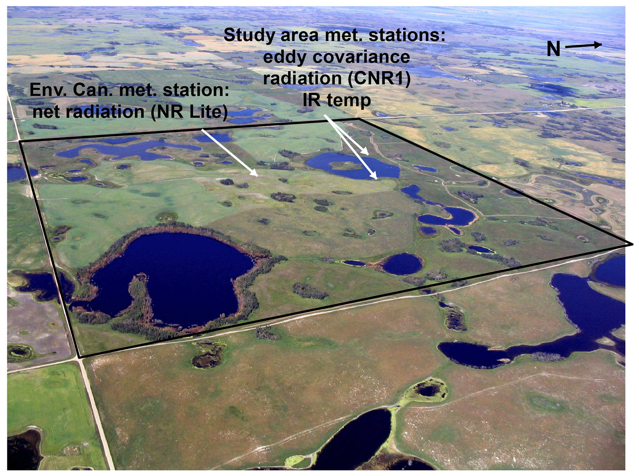
Figure 1Photo of the study area at St. Denis National Wildlife Area taken during the flight on 5 August 2007 and locations of micrometeorological measurement stations.
3.1 Granger–Gray evaporation model (G–D model)
Granger and Gray (1989) developed the G–D model from the complementary relationship of the combination model of Bouchet (1963) and Penman (1948). The G–D model extends the potential evaporation model to non-saturated surfaces using the relative evaporation term, G. This is defined as a ratio of actual to potential evaporation which depends on the relative drying power of the air, D. The underlying theory is based on the reduction of water availability as a surface dries, but the “potential” evaporation increases due to a subsequent rise in surface temperature.
The development of G eliminated the need for observations of surface temperature and vapour pressure. As a result, estimates of actual evaporation were obtainable for non-saturated surfaces with atmospheric data alone (Granger, 1989). The general form of the equation is
The available energy term is driven by net radiation, Q* (W m−2), calculated as a sum of the net shortwave and longwave radiation components and the ground heat flux, Qg (W m−2), and the slope of the saturation vapour pressure curve, Δ.
The aerodynamic term includes the psychrometric constant, γ, and “drying power of the air”, EA, calculated using a Dalton-type formula.
where f(u) is a vapour transfer function, and the atmospheric vapour pressure deficit at 2 m height is derived from (saturated) and ea (actual). Pomeroy et al. (1997) empirically derived f(u) as a function of wind speed and aerodynamic roughness length and Z0 (m) from extensive field data collected for prairie, boreal forest, and northern cold-region environments in western Canada.
where u is the mean daily wind speed (m s−1).
The G–D complementary feedback method is driven by the non-linear relationship between G and the relative drying power of the air, D.
where D is a function of the humidity deficit and available energy is given by
and λ is the latent heat of vaporisation (kJ kg−1).
The feedback model approach is generally applicable for regions indicated above and can be used when detailed soil moisture information is lacking, except under conditions of severe moisture stress. Armstrong et al. (2008) evaluated point-scale evaporation estimates obtained with the G–D model over mixed grasses at the same study area under conditions of non-limiting soil moisture using field data collected during 2006. Estimates obtained with the G–D model compared well with eddy covariance (EC) measurements and was less data intensive than the Penman–Monteith model, which also performed well in that study.
Armstrong et al. (2010), however, found that the use of appropriate soil moisture constraints was required to obtain reliable estimates with the G–D model when applied under drought conditions to a mixed-prairie site at Lethbridge, Alberta, Canada.
3.2 Field observations
Inputs needed to parameterise Eqs. (1)–(5) included mean daily net radiation, air temperature, humidity, wind speed, and surface roughness length. Outgoing radiation components were derived from high-resolution digital (Canon PowerShot A70 camera) and thermal (FLIR ThermaCAM P20 imaging radiometer) images taken on 5 August 2007 during a Cessna flight at midday. Meteorological and surface observations (radiation components, temperature, humidity, and wind speed) were recorded at two station locations. Figure 1 shows the relative locations, which included one reference site and one validation site. An independent station operated by the National Water Research Institute (Environment Canada, Saskatoon) was also available which provided a second validation site for estimates of daily net radiation. Air temperature, humidity, wind speed, incoming radiation, and surface temperature were recorded as 15 min averages. Incoming and outgoing shortwave and longwave radiation were measured with a CNR1 net radiometer (Kipp & Zonen, Delft, the Netherlands). Air temperature and humidity were measured at 2 m height using a shielded Vaisala HMP45C (Campbell Scientific, Inc., Logan, Utah, USA). A shielded Exergen infrared (IR) temperature sensor (IRTC; Exergen, Watertown, Massachusetts, USA) was used to measure surface temperature.
Canopy spectral reflectance was independently sampled on 21 August 2007 for validating albedo estimates derived from the visible images taken on 5 August. Canopy reflectance was collected according to the methods of Disney et al. (2004) and Zhang and Guo (2007). Samples were taken at 4.5 m intervals along a site transect at 1 m height at the nadir (25∘ field of view) with an ASD FR Pro spectroradiometer (Analytical Spectral Devices, Inc., Boulder, Colorado, USA); the spectral range was 350–2500 nm with a 1 nm resolution. Samples were taken between 12:00 LT (local time) and solar noon. Reflectance was recalibrated every 10 min using a white Spectralon reflectance panel (Labsphere Inc., North Sutton, New Hampshire, USA).
Eddy covariance observations were sampled at approximately 2 m height with a CSAT3 three-dimensional sonic anemometer (Campbell Scientific, Inc., Logan, Utah, USA) and a KH20 ultraviolet krypton hygrometer (Campbell Scientific, Inc., Logan, Utah, USA). The raw EC data were reported as 15 min averages and post-processing was done with MATLAB (Mathworks, Natick, Massachusetts, USA) which included flux corrections using a standard planar-fit axis rotation algorithm (Wilczak et al., 2001). Data filtering indicated there were no missing or bad data values on the study day, and station positioning was not considered to be an issue. EC data collected at the validation site were used for a comparison against a mean estimate obtained from the G–D model upwind of the EC station.
Given the higher frequency of flux reporting (15 min averages), axis rotation, and data filtering applied, and a potential mismatch in measurement footprints, no further corrections were used to force an energy balance closure on the 15 min averages.
3.3 Surface reference meteorological parameters
At midday, reference observations of the shortwave, K↓ (835 W m−2), and longwave, L↓ (320 W m−2), irradiance and albedo (0.153 over grass) were obtained from the CNR1. Both K↓ and L↓ were assumed to be uniform over the field given the images used for calculations were cloud free. The reference values were used in the calculation of midday normalised ratiometric indexes for albedo and net radiation. A mean daily reference value of 155 W m−2 was obtained for Q* which was the input for distributing the final estimates of the mean daily net radiation using the ratiometric index (discussed in Sect. 3.4).
The daily ground heat flux measured at two locations was relatively small, 8 and 2 W m−2, due to the continuous and tall grass canopy cover. For this study the ground heat flux was ignored, in part due to the small measured values, but this was also to limit errors introduced from using a numerical solution to estimate ground heat flux, which would require more-detailed cover information at each image pixel. To standardise the parameterisation of the G–D model for calculating the mean daily estimates of evaporation, the reference values of mean daily air temperature (19.6 ∘C), humidity deficit (1.1 kPa), and wind speed (3 m s−1) were also taken to be uniform. Differences in mean daily air temperature between the measurement locations were approximately 1 ∘C.
Potential impacts of assuming uniform humidity and wind speed for parameterising the aerodynamic term was also considered. This was done by examining G–D evaporation estimates derived from 2006 field data collected over different surfaces at the same study area (Armstrong et al., 2008). During 2006 a fixed station obtained continuous measurements over a mixed-grass upland, and a portable EC station was moved periodically to obtain concurrent measurements over different land covers. Meteorological observations from the fixed station were initially used to estimate evaporation with the G–D model. Another estimate was obtained after substituting observations of humidity and wind speed taken from the portable EC station. This resulted in only minor variations in the respective evaporation estimates (root mean square deviation (RMSD) of 0.02 mm) derived from the concurrent measurements of humidity and wind speed taken from the different sites.
Implications of neglecting the ground heat flux and treatment of the meteorological parameters (above) with respect to modelling uncertainty are given in the discussion.
3.4 Deriving key surface variables from one-time-of-day images
3.4.1 Theoretical basis for a normalised ratiometric index for surface properties
Remotely sensed images contain valuable information that characterise highly variable surface properties (e.g. reflectance, temperature, RGB (red–green–blue) and greyscale digital numbers (DNs), etc.). Theoretically, relative variations in these properties can be quantified using a “normalised” ratiometric index. For example, consider the “evaporation ratio” (ER), defined simply as the ratios of individual evaporation rates at different spatial locations (Ei) to a reference rate obtained at a specified location (Eref).
At the reference location ER is 1 and will be the same at any other locations where Ei=Eref, but it will vary from unity at all other spatial locations.
For obvious reasons the theory integrates well for computations with pixel-based images. Subsequently, an evaporation rate measured at the reference pixel could be scaled to all other pixels by multiplication with the value of ER at each pixel. The concept may be extended to other surface variables (e.g. albedo, net radiation, etc.) required to parameterise an evaporation model.
3.4.2 Distributing surface variables using a normalised index of relative surface ratios
Methods described here assume spatial variations in surface variables driving net radiation (and driving evaporation) are near their maximum around solar noon. This is likely to be valid within 2 h from the actual time of solar noon (Colaizzi et al., 2006). Net radiation is the major component needed to determine available energy for the conversion of water to an equivalent depth of water vapour. Net radiation is determined from the shortwave and longwave radiation components measured in the electromagnetic spectrum between approximately 0.3 and 4 and 4 and 14 µm, respectively (Zoran and Stefan, 2006).
Traditionally, radiative terms needed for estimating evaporation are derived from satellite-based imagery, e.g. Landsat, AVHRR (Advanced Very High Resolution Radiometer), and MODIS (Moderate Resolution Imaging Spectroradiometer). However, satellite-based methods are often limited by cloud contamination, varying spatial and temporal resolutions, and sensor footprint mismatches. Under clear skies it can be assumed shortwave and longwave irradiance are uniform over an agricultural field area. Very-high-resolution images taken near the surface could be used to derive the much more variable surface-reflected shortwave and emitted longwave radiation components.
For example, normalised ratiometric indexes for albedo, αR, emitted longwave, L↑R, and roughness length, , can be calculated at every pixel location within visible and thermal images using
where the subscript “i” is an individual value at each pixel and “ref” is the value at the reference pixel. Incoming shortwave (K↓) and longwave radiation (L↓) components can reasonably be assumed to be uniform over the field under clear skies, so αR and L↑R can be further integrated to derive a ratiometric index of the midday net radiation, .
Subsequently, single measured values of albedo and mean daily net radiation taken at a reference pixel can be scaled (i.e. distributed) across all other pixels via multiplication with the surface ratios derived for . The next section illustrates the indexing method for deriving accurate estimates of albedo.
3.4.3 Ratiometric-index method for albedo estimates from digital visible images
Surface albedo (α) represents a crucial radiation loss term for radiative transfer calculations and surface–atmosphere energy and mass exchanges (Sellers et al., 1997; Liang, 2000; Lucht et al., 2000; Roberts, 2001; Liang et al., 2003; Disney et al., 2004). Its calculation can be complex and is typically a major source of uncertainty (Yang et al., 2008).
In this case, a measured value of broadband albedo obtained at a reference pixel location could be scaled to every other pixel within a high-resolution visible image. In 2007, digital photos were taken with a Canon PowerShot A70 camera with a maximum resolution of 2048×1536 pixels, a CCD (charge-coupled device) imager, and a DIGIC (Digital Imaging Core) processor. This resulted in very-high-resolution (<1 m pixels) “visible images” without cloud cover issues.
While digital cameras may not cover the full visible and near-infrared spectrum of advanced measurement sensors, the imaging techniques are based on the same principles. Corripio (2004) demonstrated how accurate estimates of snow albedo could be obtained from digital images using a linear scaling technique applied to a measured albedo at a reference pixel location. A key step for our analysis was to transform an RGB digital photo to a single-band 8 bit greyscale image with DNs ranging from 0 to 255.
This resulted in higher DNs associated with more-reflective surfaces (i.e. brighter) and lower DNs with less-reflective surfaces (i.e. darker) in accordance with the principles for calculating albedo. The resulting albedo map was aggregated to a pixel size of 5 m for a practical analysis and georectified to 100 GPS ground control points. The study area included some dried wetlands and others containing open water. This allowed for application of a simple dark-object subtraction (DOS) method to correct potential atmospheric effects (Song et al., 2001; Liang, 2000).
Applying Eq. (11) made it possible to accurately estimate albedo at individual pixel locations, αi, from a measured broadband value taken at the reference location, αref, and a ratiometric index for DNs calculated at each pixel.
where DNi is the digital number of an individual pixel and DNref is the reference pixel value.
Angular measurements of broadband albedo from 0.3 to 3.0 µm with a hemispherical CNR1 directly accounted for bidirectional reflectance properties of the mixed grassed surface. Therefore, the point observations satisfied the bidirectional reflectance considerations related to albedo estimation techniques (Nicodemus et al., 1977; Lucht et al., 2000; Roberts, 2001).
Figure 2 shows a sample of measured reflectance values from a grassed upland area. The spectral reflectance from the mixed grasses was virtually identical to the response for healthy (green) winter wheat (see Disney et al., 2004). For wheat, they concluded reflectance was directionally invariant and reasonably could be assumed to behave as a Lambertian surface (i.e. scattering light equally in all directions). The field-measured spectral reflectance over the grassed surface was therefore treated similar to a Landsat-measured reflectance and divided into respective wavelengths for Landsat wavebands 1, 3, 4, 5, and 7.

Figure 2Reflectance spectra collected at four sample points over mixed-grassland vegetation at the upland area on 5 August 2007. Reflectance values affected by noise at corresponding wavelengths were removed.
An empirical linear approximation for narrow-to-broadband albedo conversion applicable to Landsat imagery (see Liang, 2000) was then applied to the field-measured spectral reflectance data. This allowed for a direct comparison of albedo estimates and measurements along the sampling transect shown in Fig. 3. Due to the 4.5 m sampling distance some pixels contained a single value, whilst others contained two values, in which case the mean value was used for comparison.
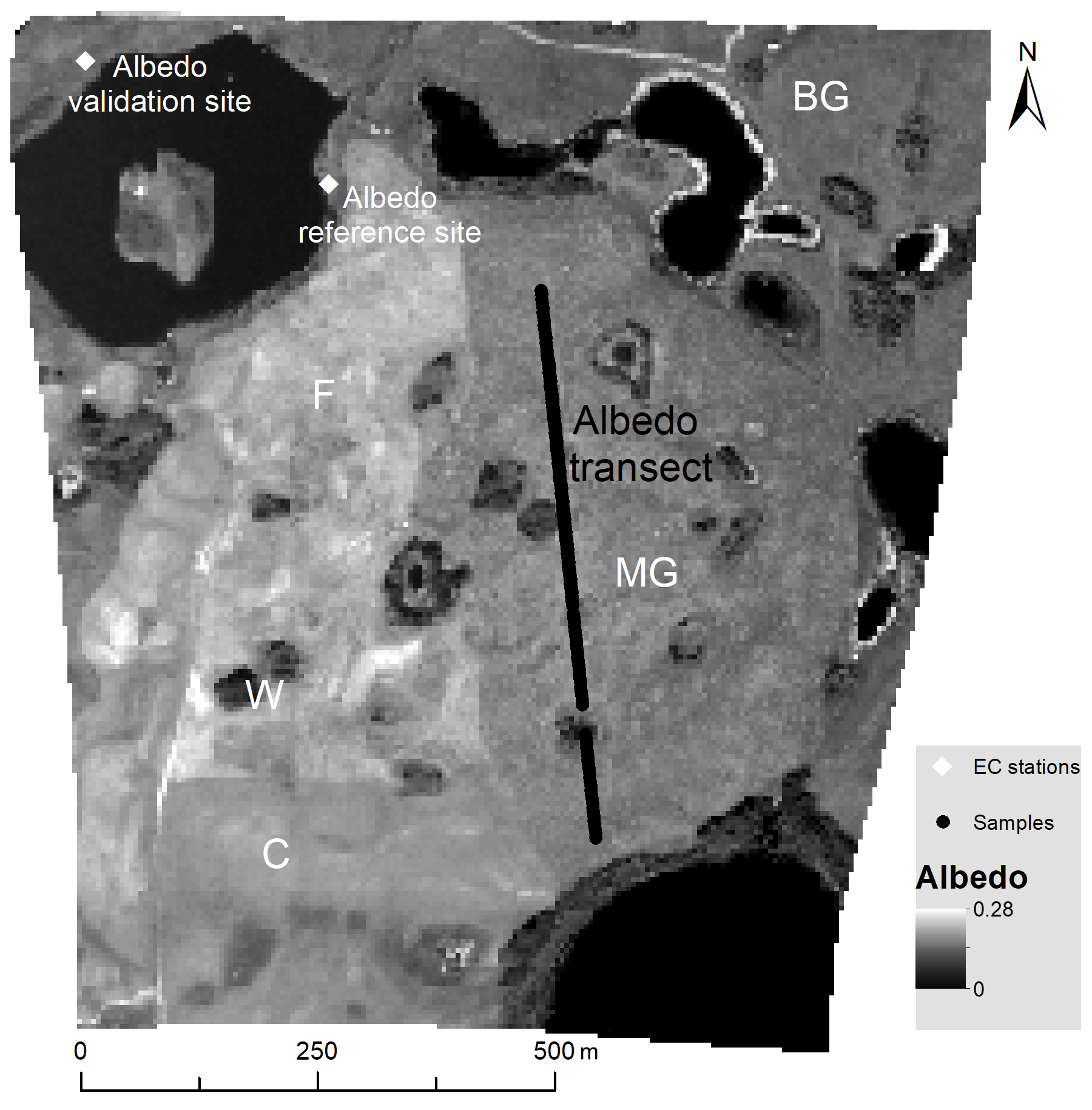
Figure 3Albedo map (5 m resolution) derived from visible images taken at midday. Also shown are the location of reference and validation sites; letter codes indicate major land cover types: fallowed (F), mixed grass (MG), brome grass (BG), cultivated (C), and wetlands (W).
3.4.4 Surface temperature (emitted longwave radiation)
For the case of surface temperatures the indexing method was not needed because high-resolution observations were obtained directly with a handheld forward-looking infrared (FLIR) ThermaCAM P20 imaging radiometer. The P20 used a focal plane array uncooled microbolometer with a maximum image resolution of 320×240 pixels, a 24∘ × 18∘ field of view, and a spatial resolution of 1.3 mrad. The spectral range was 7.5–13 µm, which is similar to traditional satellite sensors (e.g. Landsat, MODIS, and AVHRR with a spectral range of 10–12.5 µm and ASTER with a spectral range of 8–12 µm).
A standard emissivity of 0.98 was assumed for the cover types encountered, and ambient air temperature and humidity and the distance between the surface and camera detector were set based on observations. The Stefan–Boltzmann equation was applied to transform surface temperatures into values of outgoing longwave radiation needed to estimate the net radiation. For the flight height of approximately 1 km the FLIR produced a surface pixel resolution of approximately 3 m. The longwave radiation map was then aggregated to a 5 m resolution and georectified using the resulting map of albedo estimates as the reference.
3.4.5 Surface roughness length
The study area is characterised by a complex landscape with rolling terrain covered by tall grasses, cultivated land, and narrow rings of tall grasses, tall shrubs, or tall trees surrounding ponds and dried wetlands (see Fig. 1). Such surface characteristics (e.g. discontinuities and protrusions) are expected to produce variations in wind speed and turbulent energy through interactions with the different surface types and roughness.
Variations in the aerodynamic roughness length, Z0, and wind speed are important factors considered in the turbulent transfer function used for calculating the aerodynamic terms of the G–D model (Eqs. 2 and 3). Previous developments (e.g. Pomeroy et al., 1997) have considered boundary layer (friction velocity) and surface parameters (roughness length) estimated from EC measurements and wind profiles over boreal forests and Canadian Prairie land covers such as bare soil and C3-type crop and grasses.
Due to the general surface complexity at the study area, roughness classes for Z0 were needed to adjust the vapour transfer function to reflect potential increases or decreases in turbulent exchanges as result of variations in surface properties and local roughness. For example, lower values of Z0 associated with fallowed areas and crops would imply increased wind speeds near the ground and a reduction in turbulent energy. In contrast, larger Z0 values associated with taller dense grasses, shrubs, and trees would effectively reduce wind speeds and increase turbulent exchanges.
For the purposes here, a roughness length classification map for Z0 was derived from the 8 bit grayscale image used for estimating surface albedo. This was achieved based on knowledge of the various land covers at the site and segmentation analysis using the IDRISI Kilimanjaro surface analysis tool (Clark Labs, Clark University, Worcester, Massachusetts, USA). Greyscale DNs were initially classified into 13 zones of similarity, and a segmentation analysis was applied. The method computes a standard deviation for each pixel using a 3×3 moving window filter. The standard deviation and associated DN for each pixel are then sorted (low to high), and a bin range is assigned. A class width tolerance was set for pixels having similar standard deviations, and all values within a specified range were assigned to the same class. Where pixel values were outside the range, but class boundaries overlapped, a midpoint was determined and a new class was created.
The initial 13 classes were manually reclassified into three general classes (fallowed/cropped, grass, and trees) based on the extents of the dominant land cover types observed in the original and classified images. Characteristic roughness lengths, Z0, were then selected for each class based on values reported for similar surface types (Brutsaert, 1982). In this case, a value of 0.05 m was used for the fallowed/cropped class, and 0.10 m was used for the taller- and denser-grass class. Narrow rings of shrubs and trees around wetlands were also dense and much taller than the surrounding cover with heights varying from 3 to 10 m. Brutsaert (1982) reported roughness lengths between 0.2 and 0.4 m for similar type surface elements. The value of 0.40 m was chosen to reflect an expected increase in roughness and turbulent exchange due to a likely reduction in wind speed compared to the surrounding cover types.
3.5 Exploratory analysis of surface variables and evaporation estimates
Exploratory analysis of key surface variables and evaporation estimates was conducted using the R software environment (Grunsky, 2002). Data analysis consisted of boxplot summaries giving the 25th and 75th quartiles (i.e. the interquartile range) defined by the box, and an inner solid line indicating the median value was also given. Data points were plotted with jitter to reflect the density of outliers greater than 1.5 times larger or smaller than the interquartile range with the upper and lower limits defined by box whiskers.
Calculating detailed daily evaporation estimates and examining spatial scaling issues required the midday inputs and temporal-scaling function to be computed first. Analysis of midday inputs are described in Sect. 4.1–4.4. Section 4.5 and 4.6 discuss the sensitivity of the G–D model to the midday evaporation ratio and the temporal transfer function required for scaling a single measured value of mean daily radiation across a midday image. Section 4.7–4.9 discuss the accuracy of the resulting evaporation estimates, variations in statistical distributions of key driving components, and scaling implications for larger-scale evaporation estimates.
4.1 Validation of albedo estimates
At midday on 5 August 2007 a reference albedo of αref=0.153 was obtained from observed irradiance and the reflectance of shortwave radiation over the mix of green grasses. The albedo map resulting from Eq. (11) and locations of reference and validation points is shown in Fig. 3. Vegetation was similar at both EC station locations, and the scaled albedo estimate (0.164) agreed well with the measured value (0.167) at the validation site.
The validation of the mean and range of albedo estimates obtained for major land covers in Fig. 3 is summarised in Table 1. Estimates of albedo from the image compared well with values expected for grasses, agricultural crops, deciduous trees, and bare soils reported in Brutsaert (1982). The root mean square error (RMSE) of albedo estimates from the pixels and measured albedo values was approximately 3.5 %, which is within an expected error of 2 % to 5 % for research purposes (Liang, 2000).
Table 1Approximate mean values and ranges of albedo for the major land cover types.
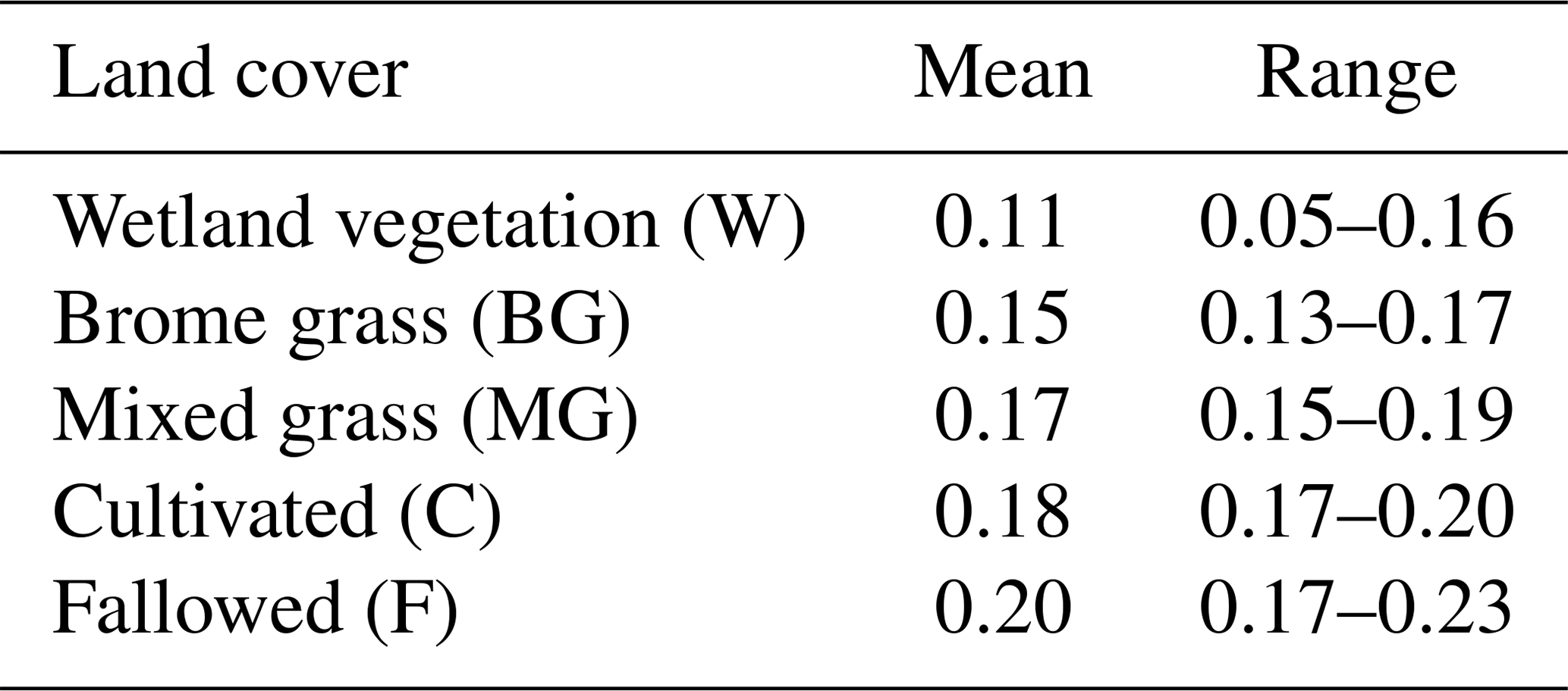
The 5 m resolution albedo map highlighted surface information within the landscape that would be more generalised using coarser data. For example, the albedo map depicted distinct boundaries separating regions dominated by brome (BG) and mixed grasses (MG), cultivated or crop area (C), sparsely vegetated, fallow area (F), and wetland fringe vegetation (W). Also, wetland extents and fringe vegetation were observable in areas surrounded by other vegetation types (see Fig. 1 for reference). The detailed variations are expected to impact evaporation estimates through relative increases at pixels with relatively lower values of albedo, which results in an increase in the available energy, whereas relatively higher values will reduce the available energy and estimates of evaporation.
4.2 Validation of longwave radiation estimates
Figure 4 shows the resulting map of emitted longwave radiation, L↑, derived from the image of observed surface temperatures, with estimates ranging between 380 to 480 W m−2. At the two EC station locations a comparison was made among the midday surface longwave measurements from the P20 camera, a narrow-beam Exergen infrared thermocouple (IRTC) radiometer, and surface-emitted longwave values obtained from the CNR1.
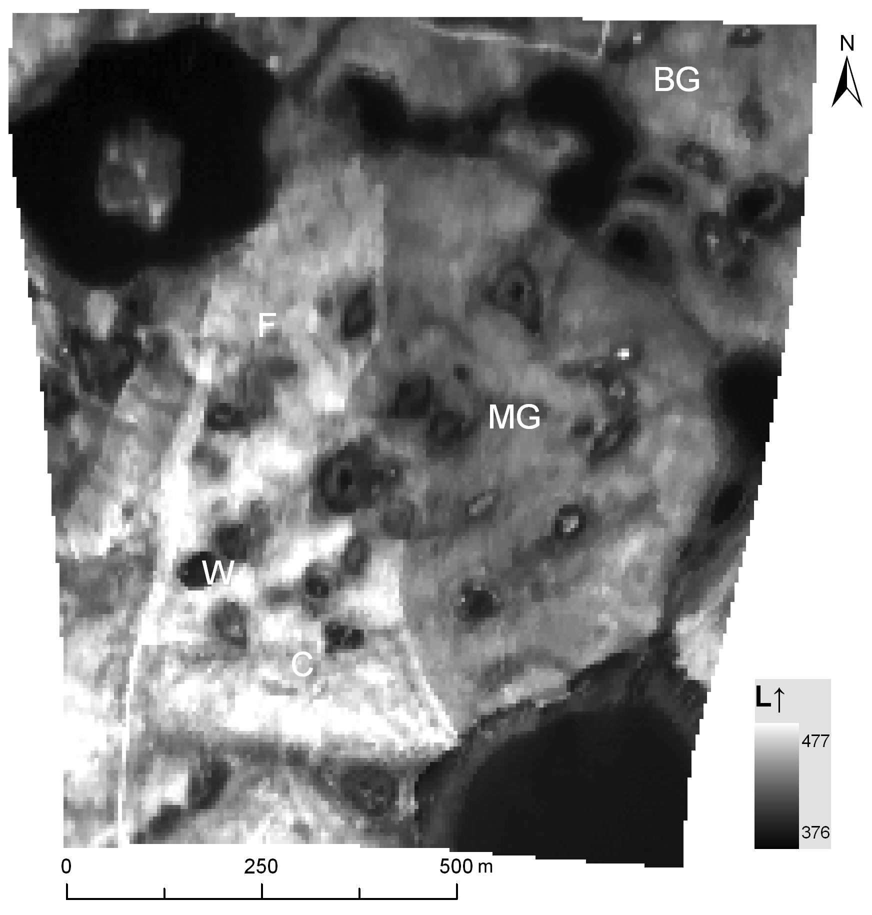
Figure 4Surface-emitted longwave radiation (W m−2) map (5 m resolution) derived from a thermal image taken at midday.
The P20 measurement compared well with the IRTC values with differences less than −12 W m−2. Compared with the CNR1 values, the differences were slightly larger at −30 W m−2 but was still within 8 % error. Generally, the differences were small considering relative changes in midday surface net radiation, and the magnitude of incoming radiation components is considerably larger. The variable footprints of the different measurements and absorption properties of water vapour, which can reduce the signal, are likely sources of error. Also, dust and heating of the CNR1 downward-facing pyrgeometer may introduce another source of error.
For estimating evaporation, the smaller emitted longwave values resulting from lower surface temperatures will increase the available energy relative to larger values which imply reduced water availability and evaporative cooling.
4.3 Surface roughness length map
Figure 5 shows the resulting classified surface roughness length, Z0, map. A visual comparison with the study area map (Fig. 1) and albedo map (Fig. 3) suggests that the classification map provides a physically realistic representation of variations in roughness over a large portion of the study area. Notable changes in the reflected surface properties and roughness length classification among the key land cover types can be observed. This is particularly true where distinct boundaries separate the transition between the dominant cover types such as where taller shrubs and trees surround ponds, compared to more broad regions of the fallow, cropped areas and grasses.
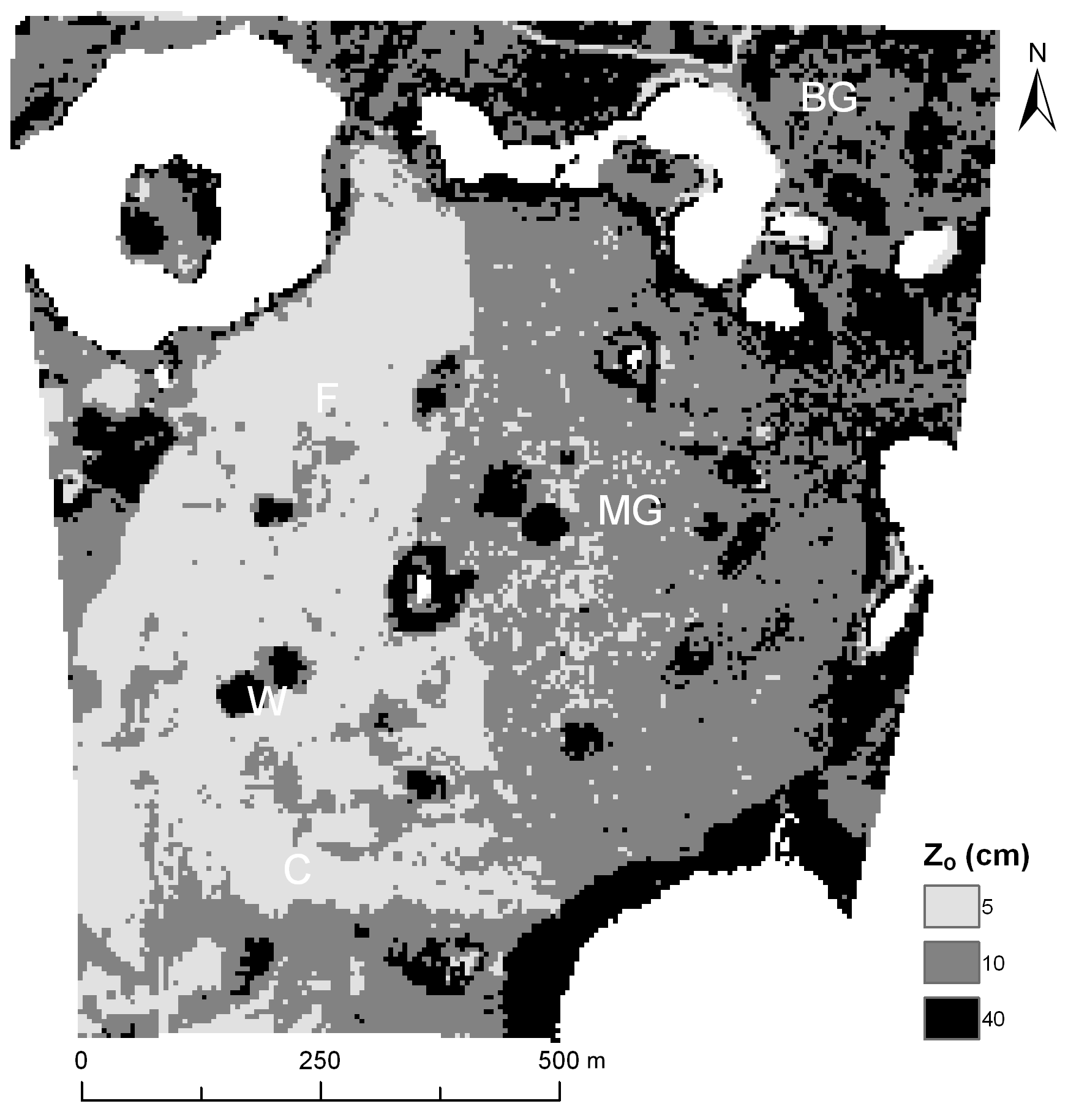
Figure 5Classification map of aerodynamic surface roughness length derived from a visible image taken at midday and typical values found in Brutsaert (1982).

Figure 6Sensitivity of the evaporation ratio to key inputs at midday. The measured range of input values is shown to demonstrate potential variation in this case study.
4.4 Sensitivity of the evaporation ratio to key variables at midday
Normalised indexes for albedo, surface temperature, and roughness were considered to examine the relationships of variations in these variables compared to the evaporation ratio. Figure 6 shows the expected physical behaviour of these variables within the G–D model. Only the actual range of values computed for the ratiometric index was considered so that the physical variations could be shown more clearly. In this case, the impacts of relative changes in the apparent inverse linear relationships between ER and αR and L↑R and slight non-linear relationship between ER and on evaporation estimates can be computed. The results can be used to illustrate the impacts of required changes in key driving variables to produce notable changes in the evaporation ratio.
For example, a relative increase in the surface temperature via L↑R of 0.18 (or 18 %) was shown to reduce ER by 10 %. By comparison, an increase in reflected shortwave radiation via αR of 0.30 (or 30 %) reduced ER by only 5 %. In the case of surface roughness, an increase of 250 % was needed to reduce ER by 10 %. Consequently, a relative reduction in evaporation rates may be expected where albedo, surface temperature, and surface roughness tend to be larger. In the latter case, step changes in surface roughness would increase the relative drying power, D, but the relative evaporation, G, results in a relative decrease due to the inverse non-linear relationship. The increased sensitivity of ER to L↑R also indicates that detailed spatial variations in surface longwave radiation is an important factor for estimating evaporation.
4.5 Temporal transfer function: normalised ratiometric radiation index
Net radiation is known to vary dynamically on a sub-daily basis. Equation (10) shows how a radiation ratio, , can be used as a temporal transfer function to scale estimates of mean daily net radiation over an image. In order to scale the normalised net radiation ratios from a temporal “point” at midday to a mean daily value, it was necessary to examine whether a stable proportionality existed between measured values at midday and mean daily net radiation. Verification of a proportionality under clear skies would eliminate the need for an empirical scaling function.
Historical records were examined for a period from 1 May to 1 September at three Canadian Prairie locations at similar latitudes (49–52.2∘). The analysis included two field seasons at the SDNWA study site (2006–2007). Archived data were also obtained at two short grass prairie locations, an AmeriFlux network site at Lethbridge, Alberta, Canada (1999–2004), and Kernen Farm located at Saskatoon, Saskatchewan, Canada (1999–2000). Figure 7 shows a moderately strong relationship at each location even with the y intercept set to 0, and r2 is equal to 0.54–0.62.
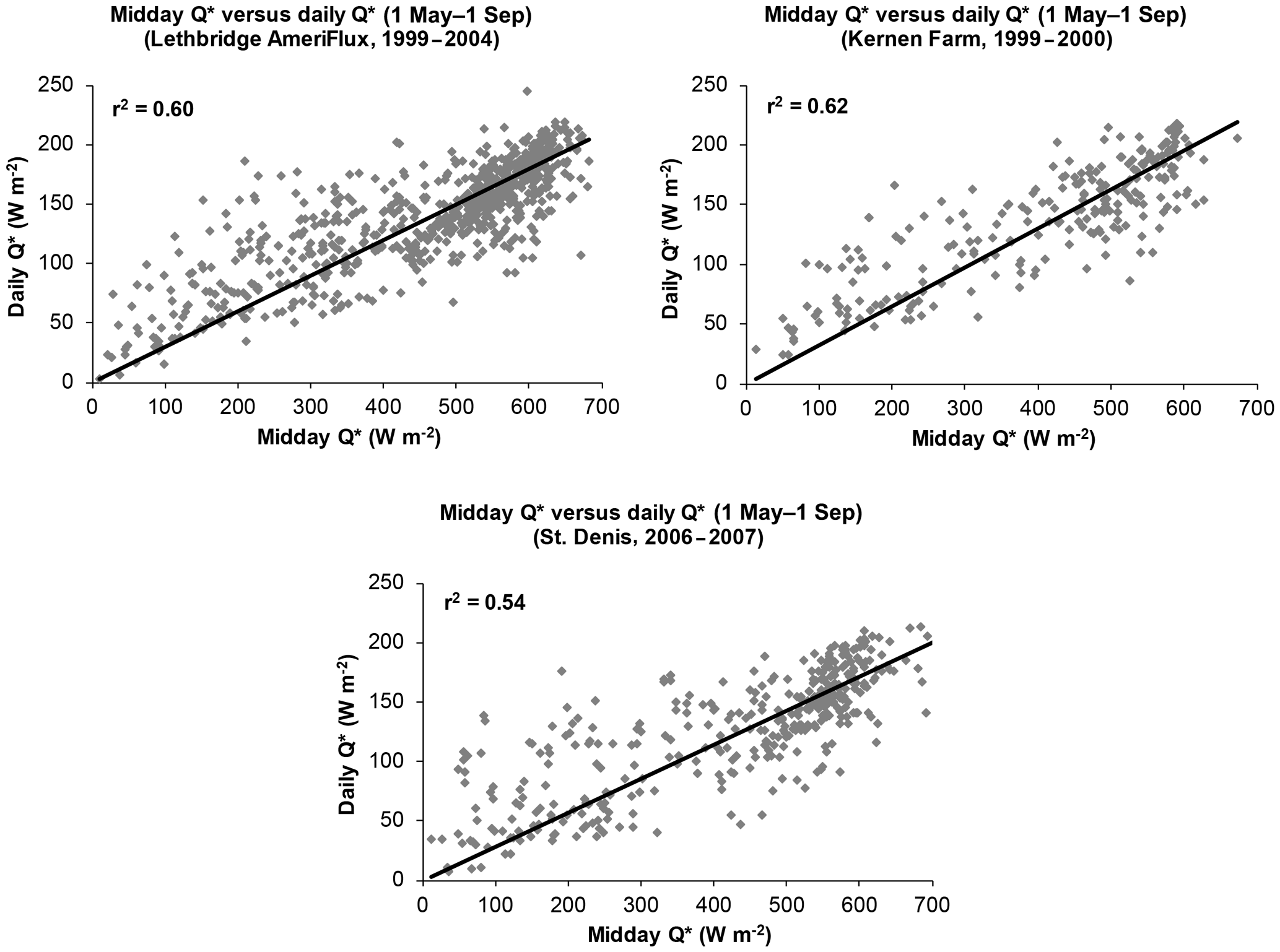
Figure 7Relationship between the midday and mean daily net radiation for a range of years at two Canadian Prairie sites and one Parkland site for the period 1 May through 1 September. R2 values shown for fitted line with the y intercept set to 0.
This result confirms that a general proportionality exists and suggests that daily net radiation, , could be scaled to all pixels across an image from a single measured reference value, , as a function of the normalised ratio index for at midday, stated here as
was assigned a daily measured reference value of 155 W m−2, which was obtained from the CNR1 at the reference station. was derived from Eq. (10) using the measured reference values of incoming shortwave and longwave radiation components, and albedo and emitted longwave maps are used as inputs. The resulting mean daily net radiation map and a comparison of estimated and measured at two validation locations are shown in Fig. 8. The main validation site was equipped with a CNR1 and a second independent site maintained by Environment Canada was equipped with an NR Lite radiometer (Kipp & Zonen, Delft, the Netherlands).
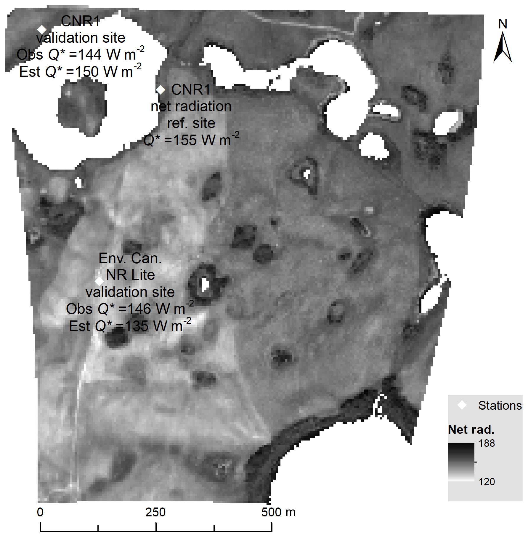
Figure 8Resulting input map of mean daily net radiation derived from the normalised index of midday net radiation and a single reference value of mean daily net radiation (155 W m−2). Also shown are the location of validation sites for comparing measured and estimated values of mean daily net radiation.
The distributed estimates of daily net radiation ranged from approximately 120 to 190 W m−2. The estimates at the validation sites were 6 W m−2 higher (4 % error) compared to the CNR1 measurement and 11 W m−2 lower (8 % error) compared to the NR Lite observation. These results indicate that accurate estimates of net radiation can be scaled across detailed midday images from a single measured value of mean daily net radiation. More importantly, detailed accurate estimates of net radiation would be valuable for improving point-scale evaporation estimates.
4.6 Calculating direct estimates of actual evaporation with the G–D model
The mean daily net radiation map derived from Eq. (12) was supplied as input to the G–D model to estimate the mean daily actual evaporation at every land surface pixel. The reference humidity and wind speed values (discussed earlier) and the surface roughness length map were used for calculating the aerodynamic terms in Eqs. (2) and (3). An estimate of mean daily evaporation was then calculated at every pixel location based on Eq. (1).
The resulting map of distributed actual evaporation estimates is shown in Fig. 9. Due to the level of detail captured in the net radiation map of Fig. 8, the map shows a physically realistic pattern of evaporation for the range of land cover types. For example, areas where vegetation was less dense (e.g. fallowed/cropped) and soil surface conditions were drier showed lower rates of mean daily evaporation, and higher rates were associated with the more-densely grassed areas. The highest evaporation estimates were obtained where water availability is expected to be higher, e.g. among wetland fringes and depressions where albedo and surface temperatures were lower, which can be attributed to increased water availability and evaporative cooling.
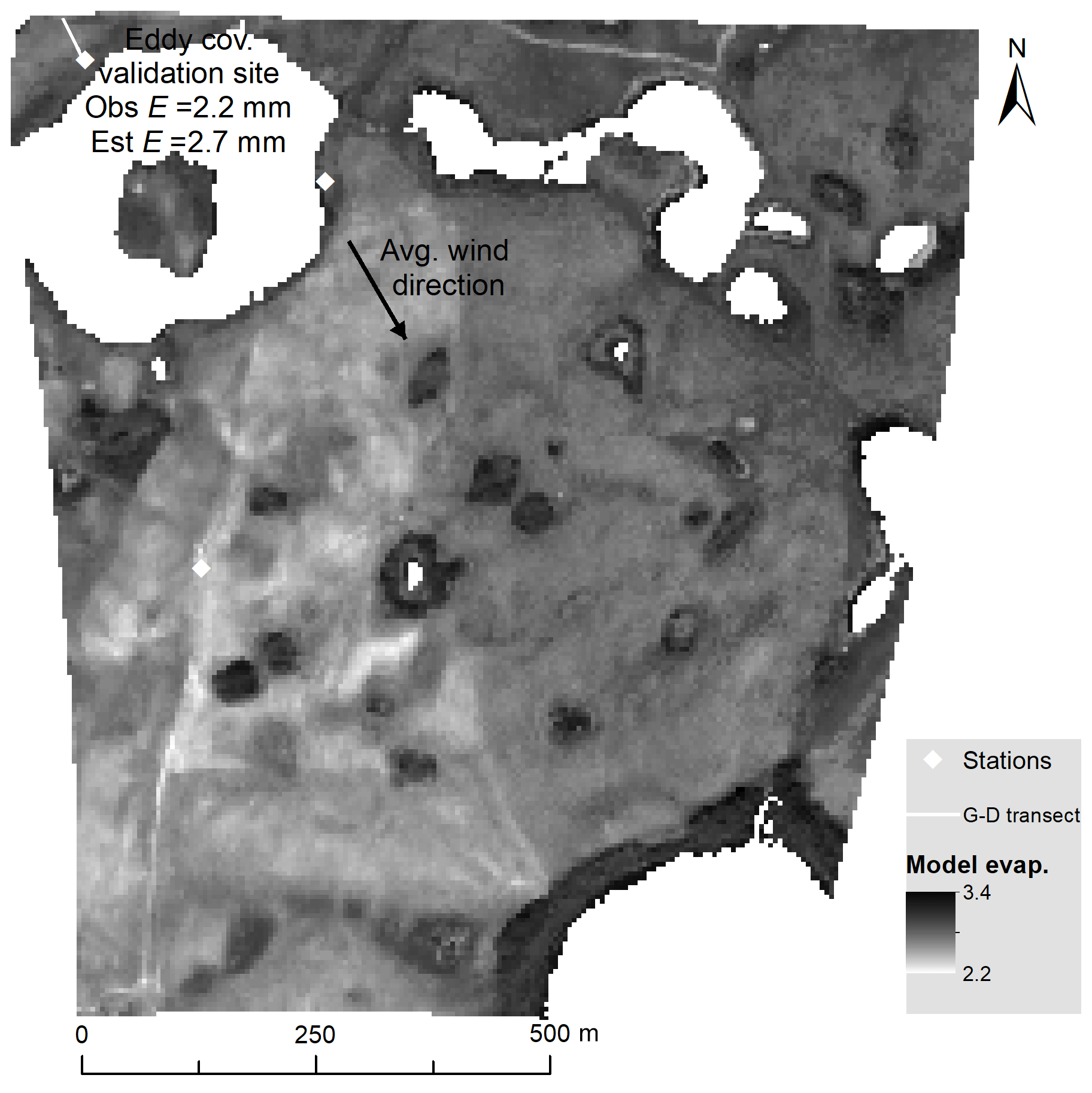
Figure 9Map of distributed estimates of mean daily evaporation at a 5 m pixel resolution.
The prevailing wind direction for the day (Udir) was from a north-northwest direction. A mean evaporation estimate of 2.7 mm was obtained along a linear transect for pixels containing a brome grass surface immediately upwind of the EC station (Fig. 9). The estimate of 2.7 mm was 0.5 mm or 23 % higher than the EC-measured mean evaporative flux of 2.2 mm d−1. Based on the cumulative flux model of Schuepp et al. (1990), it is expected that 80 % of the cumulative flux would come from within an upwind distance of 100 m from the EC station along a similar path to the linear transect. The estimate of 2.7 mm d−1 might be lower if ground heat flux was found to be a factor for reducing the available energy. However this would need to be reliably accounted for at every 5 m pixel.
On the study day the mean daily energy fluxes in W m−2 (including latent (LE) and sensible heat (HE)), and the ratio of the energy balance closure at the validation site was (LE + HE). This results in an energy balance closure of approximately 83 %. The resulting Bowen ratio of 0.87 was reasonable for the drying conditions and later timing in the growing season for the grasses in this semi-arid region. In this case it is expected there will be uncertainty in both estimated and measured EC fluxes due to modelling and measurement errors and different footprint scales. For instance, it is possible that LE and HE could be under-measured or the ground heat flux could be more variable upwind of the EC station than estimated.
Measured evaporation rates were not available for trees (dominated by aspen) in 2007, but the G–D estimates were compared against archived values from Boreal Ecosystem–Atmosphere Study (BOREAS) data for an old-aspen site from August 1996. The G–D mean daily values in the order of 3 mm were reasonable compared to evaporation from similar trees reported by Hogg et al. (2001).
In general, the results are instructive because the G–D method has been demonstrated to provide a reasonable estimate of evaporation from the remote-sensing images taken over a complex landscape. Armstrong et al. (2008) have also shown similar accuracy for daily and multi-day periods from meteorological data alone during the 2006 field season at the same study area. More importantly, the ratiometric-index method of scaling may be valid for distributing surface radiation components across remote-sensing imagery obtained from satellites, planes, or near-surface aerial platforms such as UAVs.
4.7 Distributions of evaporation and driving surface variables
The following sections briefly discuss the statistical distributions of the driving variables obtained from the images used for estimating evaporation and their impacts on the resulting evaporation estimates. The benefit here is the statistical distributions of evaporation and key driving factors are considered to be physically meaningful.
Figure 10 shows the frequency distributions of evaporation estimates and relative contributions for the energy balance and aerodynamic components. G–D model evaporation estimates appear normally distributed with a mean of 2.8 mm d−1 and a relatively low coefficient of variation (cv of 0.07). Distributions for the energy and aerodynamic terms were notably different due to interactions among the driving variables and different roughness classes. For the energy component, the distribution was continuous with a mean of 1.1 mm and a cv of 0.11. The distribution mean for the aerodynamic term was 1.7 mm and was bimodal due to the differences in magnitude of the discrete roughness classes used.
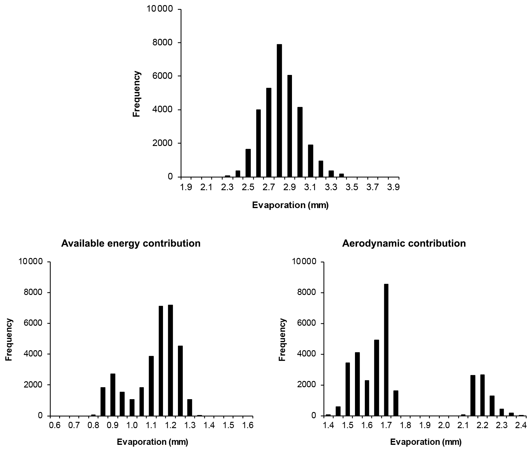
Figure 10Distribution of daily evaporation estimates over the field area and relative contributions of evaporation for the energy and aerodynamic terms.
Figure 11 shows boxplot summaries of distributions for albedo (α), surface temperature (Ts), net radiation (Q*), relative evaporation (G), mean daily evaporation (E), and G plotted against net radiation. In the case of α, values below approximately 0.10 and lower “outliers” can be attributed to uncertainty associated with the wetland vegetation and likely where surface water was not completely masked out near the edges of ponds. In general, the distributions for α and Ts which drive the net radiation appear to show more notable variability compared to Q* and the resulting estimates of E. For example, the distributions of α and Ts showed opposite skewness, −0.83 and 0.36, respectively. The variability for α (cv of 0.19) was larger than Ts (cv of 0.14), which is also much larger than apparent variability of both Q* (cv of 0.65) and E (cv of 0.66). Mean values of the distributions for α, Ts, Q*, and E were close to the median values shown within the boxes depicting the interquartile ranges.
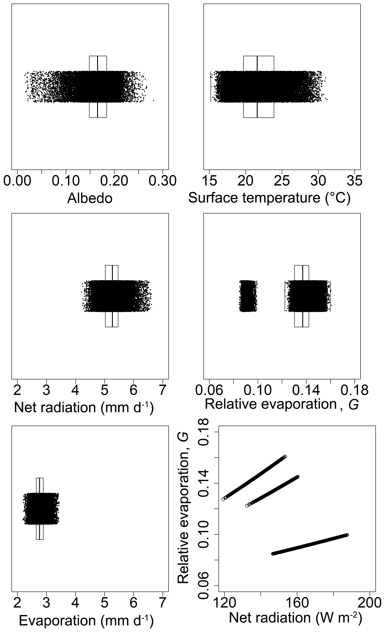
Figure 11Distribution of key surface variables, mean daily evaporation estimates, and relative evaporation over the field area and the relationship between G and net radiation within the roughness classes.
The resulting boxplot for G and the plot of G against net radiation reflects the interaction across the discrete roughness length classes. The statistical distribution of G was not continuous due to the larger step change in roughness length from 10 to 40 cm. Plots of G against net radiation resulted in three distinct linear relationships which can be attributed to using a uniform mean daily wind speed and humidity deficit for calculating the drying power of the air, EA. In this case, the potential variability of G associated with the relative drying power, D, is limited to variations in roughness length, but this may vary more with changes in wind speed and the humidity deficit.
Generally, despite the larger variability of key factors driving the energy component the complex interactions within the G–D model appear to reduce the overall variability of evaporation estimates.
Spatial variations within roughness length classes
Boxplots shown in Fig. 12 further characterise the spatial variability of α, Ts, Q*, G, and E within the three roughness length classes. In general, the plots depict notable shifts in the interquartile ranges of the distributions across the classes. Results of paired Kolmogorov–Smirnov tests for each variable showed statistical differences among the distributions for each roughness class were highly significant (p value < 0.001). General increases in albedo and surface temperature are clearly shown across the 20 to 40 cm and 10 cm roughness length classes.
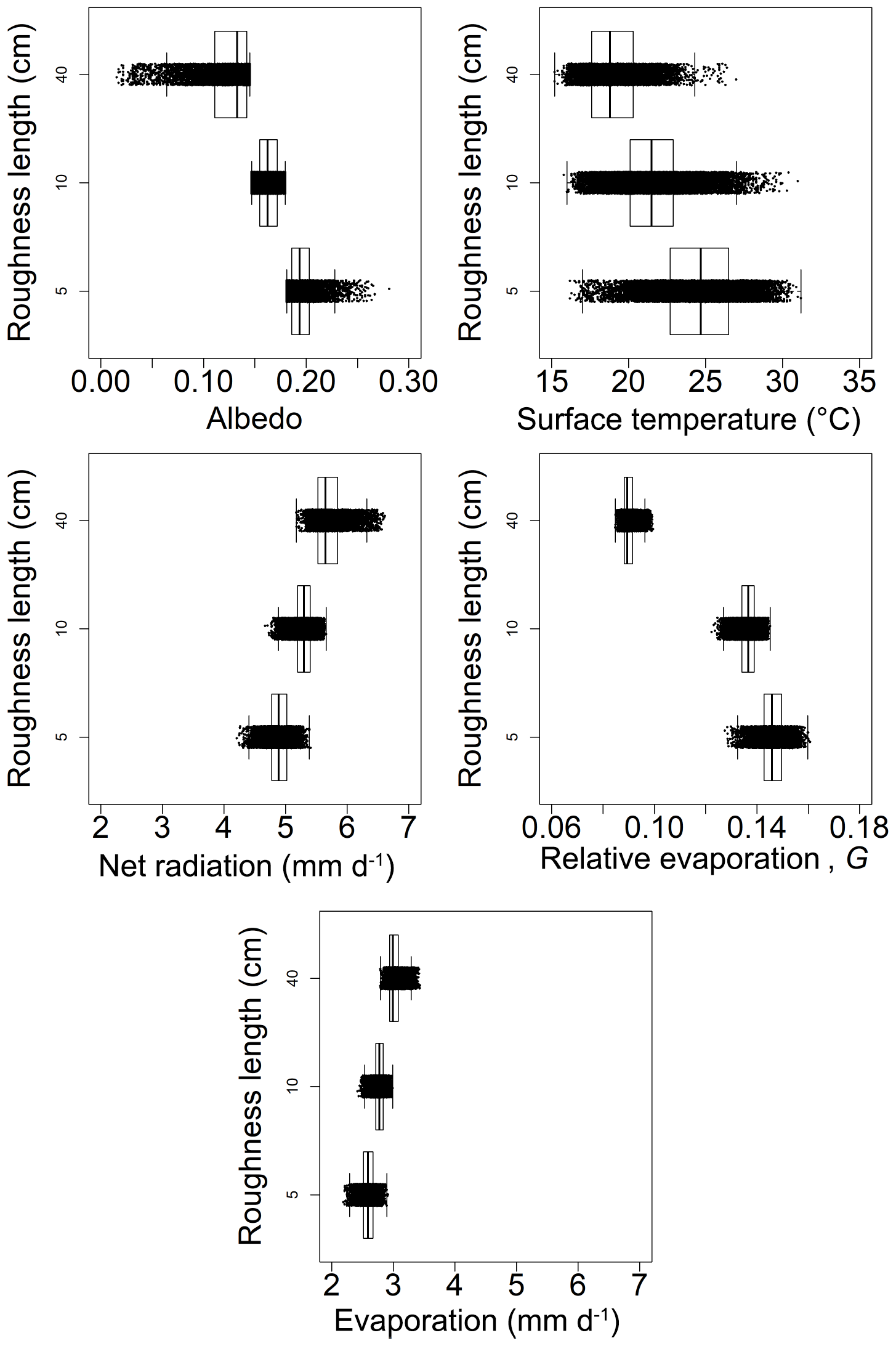
Figure 12Distributions of albedo, surface temperature, net radiation, evaporation, and relative evaporation within each roughness class.
Consequently, there was a notable reduction in net radiation and similar reduction in evaporation estimates moving from the higher to lower roughness length classes. Figure 12 also clearly shows evidence of a non-linear, inverse relationship between G and net radiation across the roughness length classes. In this case, the interaction between G and Q* appears to offset the potential increase in mean estimates of E associated with increases in available energy. As a result, a large reduction in the variability of the evaporation estimates is clearly evident when compared to the same plot for net radiation.
4.8 Scaling implications
There is a potential for areal estimates of evaporation to vary depending on how upscaled estimates are calculated from the underlying driving factors or the smaller point-scale estimates. For example, a mean areal estimate of evaporation calculated from all image pixels was 2.8 mm d−1, which accounts for all of the variability available from 5 m pixels. An areal estimate may also be calculated as a weighted mean of evaporation estimates obtained for each roughness length class. This is similar to the mosaic approach used within land surface schemes based on fractional land cover areas. The mean daily evaporation rates for the 5, 10, and 40 cm roughness length classes increased with each step change in roughness class as 2.6, 2.8, and 3.0 mm d−1, respectively. The distribution of land area associated with each roughness class was 48 % (10 cm roughness), 30 % (5 cm roughness), and 22 % (40 cm roughness). The weighted areal evaporation (Eareal) can be obtained as
In this case there was only a small difference in areal estimates obtained based on the distribution mean or a weighted mean based on fractional areas of each roughness class. This may be partly due to the relatively small variation in evaporation rates across the roughness length classes and the level of detailed variability captured by the 5 m pixel resolution. Eareal was recalculated using Eq. (13) with different combinations of the fractional areas, which only produced a minor difference of ±0.1 mm. In other words, in order for there to be a larger difference between the areal estimates, greater variability may either be required in the evaporation estimates distributed over the field or among the mean rates for each roughness class.
The mean areal estimate, Eareal of 2.8 mm d−1 for all pixels, was also 0.3 mm higher than a G–D model estimate of 2.5 mm d−1 obtained from station meteorological observations of net radiation, air temperature, humidity, and wind speed. Variations among the estimates and measurements vary by approximately 22 % to 27 %, which is not surprising given the differences in calculation techniques and potential mismatches in associated footprint scales.
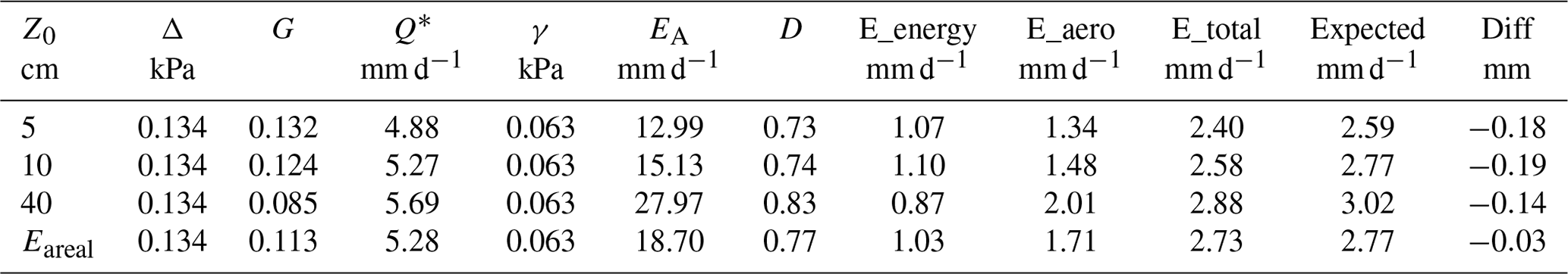
Table 2Areal evaporation estimates within each roughness class from the G–D model and for the entire area based on mean values. E_energy and E_aero are the contributions from the energy and aerodynamic components, and E_total is the combined total. The mean value of the distributed estimates is given in the column “Expected”, and the difference between the total and expected is given in the column “Diff”.
An upscaled areal mean estimate of evaporation can also be obtained from mean values of the key factors driving the energy and aerodynamic terms. The general form of Eq. (1) can be restated to derive the individual components more directly as
For the entire area and also each roughness length class, mean values of the driving factors were derived and evaporation estimates were recalculated using Eq. (14). The relative evaporative contributions attributed to the energy and aerodynamic terms are provided in Table 2. For the different roughness length classes, the range of evaporation estimates attributed to E_energy was only 0.2 mm d−1 and nearly 0.7 mm d−1 for E_aero, and the difference in total evaporation, E_total was 0.5 mm d−1. A bias toward larger evaporation estimates might be expected given the increase in energy availability and enhanced turbulence with an increase in roughness. However, the potential bias was offset by the interaction of G and Q* and also G and EA.
Table 2 also compares evaporation estimates calculated from only mean values of G and Q*, and EA to the “expected” rates for each roughness length class. Expected rates were calculated from the mean values for all pixels assigned within each roughness length class. Evaporation rates derived from the mean input values alone were only between 0.14 and 0.2 mm less than the expected mean rates for each roughness length class. Upscaling the driving factors to the entire area also had no impact on the resulting estimate as the difference was just 0.1 mm.
4.9 Examining spatial covariance among key variables
Whether evaporation estimates might be influenced by a spatial covariance between driving factors was also examined. The Pearson correlation coefficient, r, was used to evaluate correlations among the driving factors distributed over the field area. By definition, Pearson's correlation is the ratio of the covariance (the numerator) between two variables normalised by the product of their standard deviations as follows:
where Xi and Yi are the respective values of the variables, the overbar denotes the mean value, and n is the number of pairs. A strong correlation between two variables might suggest the existence of covariance that could influence upscaled estimates of evaporation. Given that the roughness classes used represent discrete data and there is a lack of more detailed meteorological data to parameterise the aerodynamic term, further evaluation related to climate factors would not be meaningful. Therefore only an examination of the factors driving the energy term are considered here.
In this case, a potential covariance between G (dimensionless) and Q* (expressed in mm d−1) can be considered directly. By rearranging Eq. (15) the covariance can be obtained by multiplying the correlation coefficient and the product of the standard deviations of Q* (0.34 mm d−1) and G (0.021 mm d−1). The correlation between Q* and G over the field area produced a coefficient, .
When multiplied in series ( this results in a covariance of approximately −0.0049 mm d−1. This suggests interactions between Q* and G for the methods applied here would have no further statistical influence on upscaled evaporation estimates. Unfortunately, no comment can be made regarding covariance between G and the turbulent flux component in the G–D model. Such analysis would require more detailed observations of air temperature, humidity, and wind speed and possibly a more sensitive combination model. Nevertheless, the impact of combined interactions within the G–D model effectively reduced the overall variability of point-scale evaporation estimates and also upscaled estimates derived from different computation methods for parameterising the model.
4.10 General uncertainty of the methods applied
Implications of general modelling assumptions and the uncertainty of the methods applied are briefly discussed here. The daily ground heat flux was considered to be negligible for the study day as the mean daily flux was relatively small at the two stations where there was good canopy coverage. Where local cover properties are similar (e.g. brome grass and mixed-grass areas) the ground heat flux may be of a similar magnitude, but it would be greater where surface cover is less dense or where water availability is limited, due to differences in the surface properties.
Further, the relative evaporation, G, which is based on the relative drying power, D, integrates available energy which in this case directly includes the spatial variability of surface temperature. As such, evaporation might be overestimated in areas with more ground exposure and higher surface temperatures, where ground heat flux may be appreciably larger (e.g. fallowed/crop area). This interaction could result in a further reduction in the energy available for the evaporation estimate.
C3-type vegetation was at the study area, but the model behaviour may differ for C4 plants and may require new vapour transfer equations for surface types and plants other than which the G–D model was developed on. In the current study representative roughness lengths were selected based on reported values for surfaces of a similar type and height. A larger uncertainty in evaporation estimates may be expected for the roughness length class associated with the shrub/tree areas which could result in variable changes in wind speed and enhanced turbulence associated with larger roughness lengths.
This study examined spatial associations and physical interactions amongst key surface variables driving actual evaporation estimates and impacts of their variations on various methods of upscaling estimates to a larger area. The methods applied demonstrate how measured reference values of albedo and mean daily net radiation can be scaled accurately across a large field area for the purpose of deriving point-scale estimates of evaporation at each pixel. This was achieved by computing a normalised ratiometric index of surface radiation from highly detailed midday visible and thermal images. At two validation sites estimates of daily net radiation showed good agreement with measured values to within 4 % and 8 % error.
Estimates of mean daily actual evaporation were calculated at 5 m resolution with the G–D model. The daily evaporation rate estimated for a transect upwind of the EC station was 2.7 mm for 5 August 2007 which was 23 % larger than the EC measured flux of 2.2 mm. Offsetting interactions between the relative evaporation term and key surface variables effectively reduce the spatial variability of evaporation estimates. As a result, differences amongst computed areal evaporation estimates were relatively small regardless of the different methods used to derive representative average values of driving factors to parameterise the model or the average evaporation rate derived from detailed estimates across the field. There was no evidence of a spatial covariance between the spatial distributions of net radiation and G, so no correction factor was identified for improving upscaled evaporation estimates.
The scaling methods applied to the energy terms using ratiometric indexes derived from detailed images could generate useful diagnostic information at other study locations and potentially over much larger areas. The methods applied here may also be instructive toward improving techniques for upscaling evaporation estimates to larger areas via traditional remote sensing or climate modelling or using a different combination model. It is expected that the methods can be applied to visible and thermal images taken from cameras and sensors on a variety of sensing platforms (e.g. satellites, planes, and UAVs).
Data used for this study can be accessed at https://doi.org/10.20383/101.0192 (Armstrong et al., 2019).
RA conducted the field investigation and modelling under the co-supervision of JP and LM. RA prepared the paper with contributions from all co-authors.
The authors declare that they have no conflict of interest.
This article is part of the special issue “Understanding and predicting Earth system and hydrological change in cold regions”. It is not associated with a conference.
We would like to extend our gratitude to the reviewers for their valuable feedback and suggested edits.
This paper was edited by Sean Carey and reviewed by two anonymous referees.
This research has been supported by the Canadian Foundation for Climate and Atmospheric Sciences through the Drought Research Initiative (DRI), the Natural Sciences and Engineering Research Council of Canada through its Discovery Grants, and the Canada Research Chairs (CRC) programme.
Anderson, M. C., Norman, J. M., Diak, G. R., Kustas, W. P., and Mecikalski, J. R.: A two-source time-integrated model for estimating surface fluxes using thermal infrared remote sensing, Remote Sens. Environ., 60, 195–216, 1997.
Anderson, M. C., Kustas, W. P., and Norman, J. M.: Upscaling flux observations from local to continental scales using thermal remote sensing, Agron. J., 99, 240–254, 2007.
Armstrong, R., Pomeroy, J., and Lawrence, M.: Evaporation modelling gridded data and meteorological station data for a case study at a rolling prairie landscape at St. Denis National Wildlife Area, Saskatchewan, Canada, https://doi.org/10.20383/101.0192, 2019.
Armstrong, R. N., Pomeroy, J. W., and Martz, L. W.: Evaluation of three evaporation estimation methods in a Canadian prairie landscape, Hydol. Process., 22, 2801–2815, 2008.
Armstrong, R. N., Pomeroy, J. W., and Martz, L. W.: Estimating Evaporation in a Prairie Landscape under Drought Conditions, Can. Water Resour. J., 35, 173–186, 2010.
Avissar, R. and Pielke, R. A.: A parameterization of heterogeneous land-surface for atmospheric numerical models and its impact on regional meteorology, Mon. Weather Rev., 117, 2113–2136, 1989.
Baldocchi, D., Falge, E., Gu, L., Olson, R., Hollinger, D., Running, S., Anthoni, P., Bernhofer, C., Davis, K., Evans, R., Fuentes, J., Goldstein, A., Katul, G., Law, B., Lee, X., Malhi, Y., Meyers, T., Munger, W., Oechel, W., Paw, K. T., Pilegaard, K., Schmid, H. P., Valentini, R., Verma, S., Vesala, T., Wilson, K., and Wofsy, S.: FLUXNET: A new tool to study the temporal and spatial variability of ecosystem-scale carbon dioxide, water vapour and energy flux densities, B. Am. Meteorol. Soc., 82, 2415–2434, 2001.
Baldocchi, D., Krebs, T., and Leclerc, M. Y.: `Wet/Dry Daisyworld': A Conceptual Tool for Quantifying Sub-Grid Variability of Energy Fluxes over Heterogeneous Landscapes, Tellus B, 57, 175–188, 2005.
Bisht, G., Venturini, V., Islam, S., and Jiang, L.: Estimation of the net radiation using MODIS (Moderate Resolution Imaging Spectroradiometer) data for clear sky days, Remote Sens. Environ., 97, 52–67, 2005.
Boegh, E., Soegaard, H., and Thomsen, A.: Evaluating evapotranspiration rates and surface conditions using Landsat TM to estimate atmospheric resistance and surface resistance, Remote Sens. Environ., 79, 329–343, 2002.
Bouchet, R. J.: Evapotranspiration réelle et potentielle: Signification climatique, General Assembly, Berkeley, Int. Assoc. Sci. Hydrol., 62, 134–142, 1963.
Brutsaert, W.: Evaporation into the Atmosphere, D. Reidel, Hingham, Massachussetts, 299 pp., 1982.
Brutsaert, W.: Land-surface water vapor and sensible heat flux: Spatial variability, homogeneity, and measurement scales, Water Resour. Res., 34, 2233–2442, 1998.
Bussières, N., Granger, R., and Strong, G.: Estimates of Regional Evapotranspiration using GOES-7 Satellite Data: Saskatchewan Case Study, July 1991, Can. J. Remote Sens., 23, 3–14, 1996.
Claussen, M.: Estimation of areally averaged surface fluxes, Bound.-Lay. Meteorol., 54, 387–410, 1991.
Claussen, M.: Flux aggregation at large scales: on the limits of validity of the concept of blending height, J. Hydrol., 166, 371–382, 1995.
Colaizzi, P. D., Evett, S. R., Howell, T. A., and Tolk, J. A.: Comparison of five models to scale daily evapotranspiration from one-time-of-day measurements, Am. Soc. Agr. Biol. Eng., 49, 1409–1417, 2006.
Corripio, J. G.: Snow surface albedo estimation using terrestrial photography, Int. J. Remote Sens., 25, 5705–5729, 2004.
Courault, D., Seguin, B., and Olioso, A.: Review on estimation of evapotranspiration from remote sensing data: From empirical to numerical modelling approaches, Irrig. Drain. Syst., 19, 223–249, 2005.
Disney, M., Lewis, P., Thackray, G., Quaife, T., and Barnsley, M.: Comparison of MODIS broadband albedo over an agricultural site with ground measurements and values derived from Earth observation data at a range of spatial scales, Int. J. Remote Sens., 25, 5297–5317, 2004.
Fisher, J. B., Tu, K. P., and Baldocchi, D. D.: Global estimates of the land-atmosphere water flux based on monthly AVHRR and ISLSCP-II data, validated at 16 FLUXNET sites, Remote Sens. Environ., 112, 901–919, 2008.
Gowda, P. H., Chavez, J. L., Colaizzi, P. D., Evett, S. R., Howell, T. A., and Tolk, J. A.: ET mapping for agricultural water management: present status and challenges, Irrig. Sci., 26, 223–237, 2007.
Granger, R. J.: A complementary relationship approach for evaporation from nonsaturated surfaces, J. Hydrol., 111, 31–38, 1989.
Granger, R. J.: Satellite-derived estimates of evapotranspiration in the Gediz Basin, J. Hydrol., 229, 70–76, 2000.
Granger, R. J. and Gray, D. M.: Evaporation from natural nonsaturated surfaces, J. Hydrol., 111, 21–29, 1989.
Grunsky, E.: R: A data analysis and statistical programming environment – an emerging tool for the geosciences, Comput. Geosci., 28, 1219–1222, 2002.
Hogg, E. H., Price, D. T., and Black, T. A.: Postulated Feedbacks of Deciduous Forest Phenology on Seasonal Climate Patterns in the Western Canadian Interior, J. Climate, 13, 4229–4243, 2001.
Houborg, R. M. and Soegaard, H.: Regional simulation of ecosystem CO2 and water vapor exchange for agricultural land using NOAA AVHRR and Terra MODIS satellite data. Application to Zealand, Denmark, Remote Sens. Environ., 93, 150–167, 2004.
Jackson, R. D., Reginato, R. J., and Idso, S. B.: Wheat canopy temperature: a practical tool for evaluating water requirements, Water Resour. Res., 13, 651–656, 1977.
Klaassen, W.: Average fluxes from heterogeneous vegetated regions, Bound.-Lay. Meteorol., 58, 329–354, 1992.
Klaassen, W. and Claussen, M.: Landscape variability and surface flux parameterization in climate models, Agr. Forest Meteorol., 73, 181–188, 1995.
Liang, S.: Narrowband to broadband conversions of land surface albedo: I. Algorithms, Remote Sens. Environ., 76, 213–238, 2000.
Liang, S. L., Shuey, C. J., Russ, A. L., Fang, H. L., Chen, M. Z., Walthall, C. L., Daughtry, C., and Hunt, R.: Narrowband to broadband conversions of land surface albedo: II. Validation, Remote Sens. Environ., 84, 25–41, 2003.
Lucht, W., Schaaf, C. B., and Strahler, A. H.: An algorithm for the retrieval of albedo from space using semiempirical BRDF models, IEEE T. Geosci. Remote, 38, 977–998, 2000.
Monteith, J. L.: Evaporation and environment, Symp. Soc. Exp. Biol., 19, 205–234, 1965.
Mu, Q., Heinsch, F. A., Zhao, M., and Running, S. W.: Development of a global evapotranspiration algorithm based on MODIS and global meteorology data, Remote Sens. Environ., 111, 519–536, 2007.
Nagler, P. L., Cleverly, J. R., Glenn, E. P., Lampkin, D., Huete, A. R., and Wan, Z.: Predicting riparian evapotranspiration from MODIS vegetation indices and meteorological data, Remote Sens. Environ., 94, 17–30, 2005.
Nicodemus, F. E., Richmond, J. C., Hsia, J. J., Ginsberg, I. W., and Limperis, T.: Geometrical considerations and nomenclature for reflectance, Report, National Bureau of Standards, Washington, D.C., p. 67, 1977.
Norman, J. M., Kustas, W. P., and Humes, K. S.: Source approach for estimating soil and vegetation energy fluxes in observations of directional radiometric surface temperature, Agr. Forest Meteorol., 77, 263–293, 1995.
Penman, H. L.: Natural evaporation from open water, bare soil and grass, P. Roy. Soc. Lond. A, 193, 120–146, 1948.
Pomeroy, J. W., Granger, R. J., Pietroniro, A., Elliott, J. E., Toth, B., and Hedstrom, N.: Hydrological Pathways in the Prince Albert Model Forest, Final Report to the Prince Albert Model Forest Association, NHRI Contribution Series No. CS-97004, Environment Canada, NHRI, Saskatoon, p. 154 + appendices, 1997.
Roberts, G.: A review of the application of BRDF models to infer land cover parameters at regional and global scales, Prog. Phys. Geogr., 25, 483–511, 2001.
Schuepp, P. H., Leclerc, M. Y., McPherson, J. I., and Desjardin, R. L.: Footprint prediction of scalar fluxes from analytical solutions of the diffusion equation, Bound.-Lay. Meteorol., 50, 355–374, 1990.
Seguin, B., Assad, E., Freaud, J. P., Imbernon, J. P., Kerr, Y., and Lagouarde, J. P.: Use of meteorological satellite for rainfall and evaporation monitoring, Int. J. Remote Sens., 10, 1001–1017, 1989.
Sellers, P. J., Dickinson, R. E., Randall, D. A., Betts, A. K., Hall, F. G., Berry, J. A., Collatz, G. J., Denning, A. S., Mooney, H. A., Nobre, C. A., Sato, N., Field, C. B., and Henderson-Sellers, A.: Modelling the exchanges of energy, water, and carbon between continents and the atmosphere, Science, 275, 502–509, 1997.
Song, C., Woodcock, C. E., Seto, K. C., Lenney, M. P., and Macomber, S. A.: Classification and Change Detection Using Landsat TM Data: When and How to Correct Atmospheric Effects?, Remote Sens. Environ., 75, 230–244, 2001.
van der Kamp, G., Hayashi, M., and Gallén, D.: Comparing the hydrology of grassed and cultivated catchments in the semi-arid Canadian prairies, Hydrol. Process., 17, 559–575, 2003.
Wilczak, J. M., Oncley, S. P., and Stage, S. A.: Sonic anemometer tilt correction algorithms, Bound.-Lay. Meteorol., 99, 127–150, 2001.
Yang, F., Mitchell, K., Hou, Y.-T., Dai, Y., Zeng, X., Wang, Z., and Liang, X.-Z.: Dependence of Land Surface Albedo on Solar Zenith Angle: Observations and Model Parameterization, J. Appl. Meteorol. Clim., 47, 2963–2982, 2008.
Yates, T. T., Si, B. C., Farrell, R. E., and Pennock, D. J.: Probability distribution and spatial dependence of nitrous oxide emission: temporal change in a hummocky terrain, Soil Sci. Soc. Am. J., 70, 753–762, 2006.
Zhang, C. and Guo, X.: Measuring biological heterogeneity in the northern mixed grassland: A remote sensing approach, Can. Geogr., 51, 462–474, 2007.
Zoran, M. and Stefan, S.: Atmospheric and spectral corrections for estimating surface albedo from satellite data, J. Optoel. Adv. Mater., 8, 247–251, 2006.